
Modeling of Ion Exchange Processes to Optimize Metal Removal from Complex Mine Water Matrices
by
 ,
,
Angela Isabel Pedregal Montes
*, 
Janith Abeywickrama
,
Nils Hoth
,
Marlies Grimmer
and
Carsten Drebenstedt
Working Group Mine Water Management, Institute of Mining and Special Construction Engineering, TU Bergakademie Freiberg, Gustav-Zeuner-Straße 1a, 09599 Freiberg, Germany
*
Author to whom correspondence should be addressed.
Water 2021, 13(21), 3109; https://doi.org/10.3390/w13213109
Submission received: 28 September 2021
/
Revised: 1 November 2021
/
Accepted: 2 November 2021
/
Published: 4 November 2021
(This article belongs to the Section Wastewater Treatment and Reuse)
Abstract
:The modeling of ion exchange processes could significantly enhance their applicability in mine water treatment, as the modern synthetic resins give unique advantages for the removal of metals. Accurate modeling improves the predictability of the process, minimizing the time and costs involved in laboratory column testing. However, to date, the development and boundary conditions of such ion exchange systems with complex mine waters are rarely studied and poorly understood. A representative ion exchange model requires the definition of accurate parameters and coefficients. Therefore, theoretical coefficients estimated from natural exchange materials that are available in geochemical databases often need to be modified. A 1D reactive transport model was developed based on PhreeqC code, using three case scenarios of synthetic mine waters and varying the operating conditions. The first approach was defined with default exchange coefficients from the phreeqc.dat database to identify and study the main parameters and coefficients that govern the model: cation exchange capacity, exchange coefficients, and activity coefficients. Then, these values were adjusted through iterative calibration until a good approximation between experimental and simulation breakthrough curves was achieved. This study proposes a suitable methodology and challenges for modeling the removal of metals from complex mine waters using synthetic ion exchange resins.
1. Introduction
Given the environmental, social, and economic benefits of reprocessing mine waters, many treatment technologies have been developed to reuse water and recover resources such as metal ions [1,2,3]. Ion exchange (IX) resins technology has emerged as a promising alternative given its high selectivity for metal removal, small concentrated output volume, high quality of treated water, and the great advantage that it is a reversible and reusable process [4,5,6,7]. Some challenges to be considered when using resins for mine water treatment are the hydraulic blocking of the material due to the presence of colloids in the water or their formation by the oxidation of iron, manganese, or other metals [8]. The variation of pH in the process, depending on the type of exchange material, and the presence of calcium and sulfates in the water can develop secondary precipitations, which considerably reduce the capacity of the resin, modify the water flow inside the exchange column, and reduce the recovery process efficiency [9]. However, these difficulties can be minimized with proper pretreatment of the water, monitoring of process parameters, and upward flow of the inlet solution [4,5,6].
Although laboratory testing is vital for small-scale research, it involves sampling, analysis, and monitoring, becoming time consuming and costly [10]. Therefore, once sufficient data have been obtained from experimental tests, it is necessary to visualize the system through an ion-exchange model, which would help to describe the exchange of ions onto resins and study its behavior and performance [11]. Hydrogeochemical modeling helps to understand complex processes and is a powerful tool for assessing detailed geochemical reactions and transport processes [12]. Since the early 1970s, many authors have developed different computer programs and databases for hydrogeochemical modeling [13]. In this study, the software PhreeqC has been selected. This computer program has been evolving and increasing its capabilities over time, being able to model and simulate surface-controlled reactions such as IX and reactive mass transport in a 1D column [14]. On the other hand, PhreeqC is a public domain software, which facilitates its use and expands its scope [15].
There is a considerable amount of research on the modeling of reactive mass transport processes in natural environments, where the focus is the study of different phenomena such as solute transport, soil and freshwater contamination, and seawater intrusion [13,14,16,17,18,19]. However, surprisingly little information is available regarding the selective removal of metals from mine waters using manufactured resins [20]. Chelating resins have been developed for a broad range of applications using mine waters due to their high exchange capacity and remarkable performance at low pH values [9,21,22]. In addition, weakly basic resins with a chelating bis-picolylamine functional group possess high selectivity for metal ions with economic potential such as copper, zinc, and nickel captured from acidic solutions [23,24].
Although the theoretical cation exchange capacity (CEC) is provided by the resin manufacturer, this value differs in practice, as it depends on the operating conditions of the system [5,25]. On the other hand, the selectivity of a resin can be defined by using exchange coefficients. These coefficients have been obtained from several experimental measurements of different soils and clay minerals, and their values are defined in existing geochemical software databases [26]. Nevertheless, these default values are not always suitable for the modeling given their dependence on the characteristics of the resin and the mine water composition [26,27,28,29]. Furthermore, each ion of the inflow solution involved in the IX process requires the definition of its exchange coefficient. Otherwise, it will not be considered in the model [15]. This is why the more complex the mine water composition, the more unknowns to estimate [13]. This complexity is reflected in the limited literature on modeling IX processes using one, two, or up to three competing ions in the input solution [2,7,11,16,17,30]. Therefore, in order to address the study of more complex mine water matrices, this research contemplates a parallel work between laboratory and simulation to reduce simplifications and assumptions.
The outcomes of this project propose a well-organized methodology for a deeper assessment and support of IX column experiments using a model-based approach. Through this study, the main parameters that significantly influence the IX model have been identified and estimated for further extension and upgrading. In addition, as part of a simulation modeling, the developed model can be used to (i) predict the selective removal of metals from complex mine water matrices reducing the costs of laboratory tests and chemical analysis, (ii) speed up the study of cases over a long period of time, and (iii) upscale [31]. Subsequently, it is expected to include the resin regeneration phase in the model to simulate the process of recovery of metal ions.
2. Materials and Methods
2.1. General Approach
The model developed represents the loading phase for the selective removal of metals from acid mine drainage by IX column tests. For the first part of the study, the model was structured, tested, and improved using parameters from column experiments identified as Scenario 1 and Scenario 2, combined with default coefficient values from the PhreeqC program for geochemical calculations. Once the behavior of the parameters was identified, we proceeded to adjust their values through iterative calibration of the coefficients according to the selectivity ranks of each scenario. Due to the availability of analytical solutions, the accuracy of the model has been evaluated by making comparisons with experimental data. Subsequently, Scenario 3 was proposed for the prediction of results using the developed model. Finally, the results of the prediction have been validated by setting up this scenario at a laboratory scale to compare the breakthrough curves (BTC) of the ions contained in the solution [30].
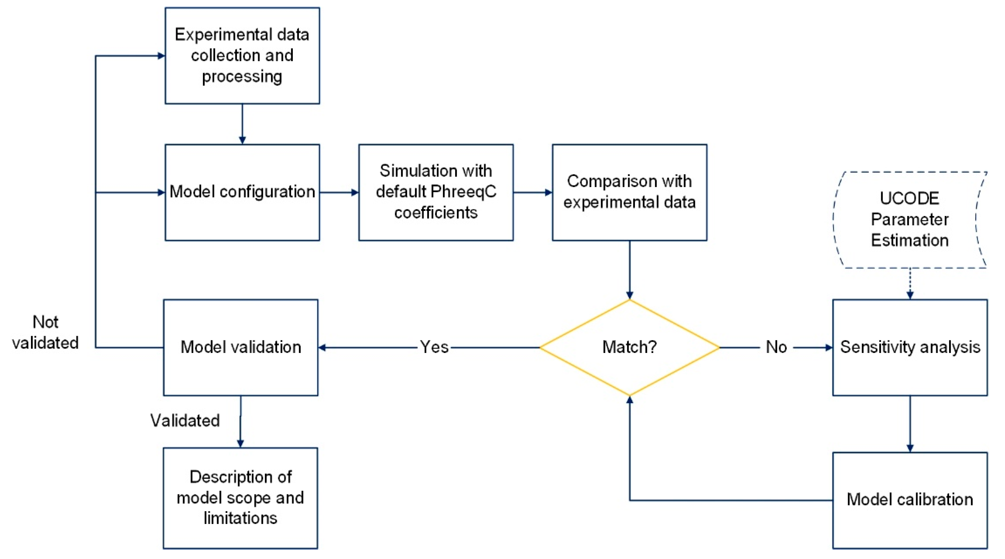
The three scenarios performed along this study required adjustments and assumptions to compensate for the uncertainty of experimental data and/or undefined species in the program database. The verification of the model was done throughout the whole process. Moreover, Figure 1 shows the flow diagram applied in this study, where the simulation modeling is both iterative and circular, given the possibility of a continuous improvement through simulation. To the process shown in Figure 1, an extra block has been added in dashed lines representing the use of the UCODE program, which performs inverse modeling, resulting in a powerful tool for model calibration and parameter estimation [32]. Although this tool was not applied to this study, it is expected to be used in future investigations for more complex systems with many unknown parameters.
2.2. Materials
Three scenarios were selected based on different aspects: (1) different complexities regarding the composition of the inflow solution, (2) different column geometry and operating conditions, and (3) same IX resin with the functional group bis-picolylamine. It is important to note that the three scenarios worked with synthetic mine waters as inflow, which were prepared based on real case studies. Therefore, working with this type of water was preferred, since complete information on its chemical composition is available. Finally, the order in which the scenarios were applied was from less to more complex in terms of the composition of the input solution: 2-cation, 4-cation, and 6-cation systems. This approach was selected as a starting point with the aim of increasing the complexity of mine water progressively due to the large number of unknowns in the model. Once the model is studied and defined, it can be applied to more complex matrices. The compositions of the three inflow waters are described in Table 1.
The sulfate concentration for Scenarios 1 and 2 was calculated through PhreeqC, and in the case of Scenario 3, the experimental value was adjusted to achieve the appropriate charge balance before proceeding with the IX simulations.
Within the wide range of chelating resins, Lewatit MonoPlus TP-220 with bis-picolylamine functional groups was selected due to its high efficiency for the removal of base metals such as copper, zinc, nickel, cobalt, and also for the removal of noble metals such as palladium, platinum, and gold, which are metals with high economic value [22]. Studies have verified the superior performance and high operational capacity of this resin compared to other exchange materials, especially in acidic conditions such as mine water [21,22,24,25,33,34,35].
The selection of a resin establishes two characteristics within the process: (1) the functional group that governs the ion exchange, which in this case is bis-picolylamine for metal cation exchange, and (2) the counter-ion that defines the composition and pH of the output solution [22,25]. The selected resin is fully protonated, so the output solution will remain in acidic conditions [23]. The description of the selected resin can be found in Table 2. According to the product information sheet, it presents a minimal exchange capacity in grams of copper per liter of resin. The selectivity rank shown for each scenario is based on experimental tests, and it can be seen that there is a difference with respect to cobalt ion between the range provided by the supplier and Scenario 2. This reinforces that the theoretical properties of the exchanger material are not constant, as mentioned previously.
2.3. Column Tests
A loading process consists of injecting an inflow solution with specific cations of a known concentration into a resin column that has a known initial composition and CEC. The resin is gradually exhausted, and the process stops when complete exhaustion is reached [5]. The experimental system is illustrated in Figure 2, where the composition of the inflow solutions was progressively increased in each scenario.
One of the best approaches to monitor an IX process is through a BTC, which is constructed by plotting the concentration of ions in the outflow solution versus time or throughput volume, which is also known as bed volume (BV) [26].
Although the bis-picolylamine exchanger material was selected for all scenarios, the operating conditions vary in all experiments in order to test the capabilities of the model. Table 3 describes the column geometry and main hydraulic characteristics for all scenarios used to define the transport data block of PhreeqC. It should be noted that the flow rate was not constant for Scenarios 1 and 2, varying during the day and night.
2.4. Analysis
The ion content analysis was performed using a microwave plasma atomic emission spectrometer (MP-AES 4200). The sulfate concentration was obtained indirectly through analyzing the total sulfur content by MP-AES.
A WTW Multimeter was used for the measurement of pH, electrical conductivity (EC), redox potential, and temperature of the water samples before, during, and after the IX loading phase.
2.5. Model and Calculations
The computer program selected for this study was PhreeqC v3 because it calculates reactive transport in one dimension and the solution of IX problems. The PhreeqC code defines cation exchange according to the Gaines–Thomas convention. The desired one-dimension model can describe the behavior of the loading phase of a cation exchange resin column with volume, time, and/or distance [15,36].
2.5.1. Fixed-Bed Model
The approach that is used to describe IX processes considers real transport conditions by using the Advection–Reaction–Dispersion (ARD) equation, which combines the processes involved. The ARD equation is shown in Equation (1) [26,37].
where c represents the solute concentration (mol/L), v is the pore water flow velocity (m/s), DL is the hydrodynamic dispersion coefficient (m2/s), and q represents the concentration in the solid (mol/L of pore water).
2.5.2. Ion Exchange Equilibrium
Due to the reversibility characteristic of an IX process, it is possible to describe it by the law of mass action [12,32,37]. The distribution of species in equilibrium is given by Equation (2) and follows the Gaines–Thomas convention that is used to calculate the IX reactions in PhreeqC [38].
where A+ and M+ are positively charged ions and represent the exchanger. The selectivity or exchange coefficient KM/A is considered the equilibrium constant of the IX reaction and defines the order of selectivity among all the ions that compose the feed solution [26,38]. Nevertheless, exchange coefficients are not constant, and their values depend on operating conditions such as concentration of inflow solutions, pH, characteristics of the resin, or the presence of competing ions in the system. Two ions with similar charges lead to similar coefficients as well [5,28].
The square brackets in Equation (2) represent the activity of the species. However, there are many theories and models to calculate activity coefficients; the Debye–Hückel theory, which is used by default for PhreeqC, relates concentrations and activities in the water. Both the exchange and activity coefficients require selecting a geochemical database to define their values in the system. The phreeqc.dat database was selected for this study, as it contains the majority of the ions present in the solutions. The database selected follows an ion-association aqueous model. Therefore, the Debye–Hückel equation requires the definition of two ion-specific parameters (a and b) to calculate the activity coefficient that will later be multiplied by its equivalent fraction to finally obtain the activity of the exchange specie. The calculation of activities through this equation is entirely empirical in order to establish a better fit with experimental data [15].
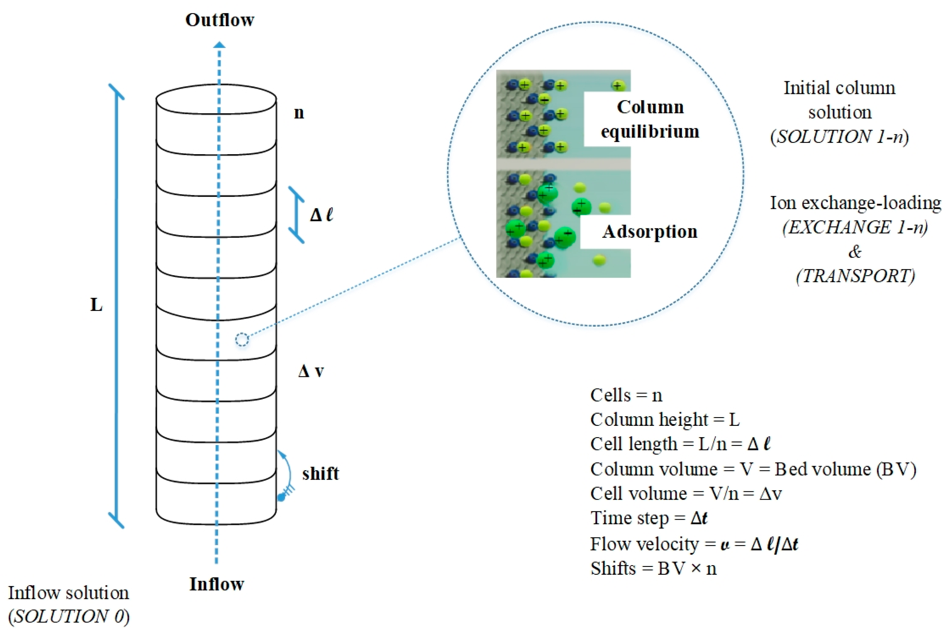
The PhreeqC code connects the fixed-bed column transport and the IX equilibrium using a 1D flowline divided by a known number of cells (n) for the column discretization. These cells are linked to the aqueous solutions (SOLUTION 1-n; SOLUTION 0) defined in the same model and can be assigned individually or in clusters. The conceptual model for this study is shown in Figure 3, where the column of height (L) is split into n cells and is composed of a single layer along the column representing the resin. The reactions occur in a series of sequential cells with identical geometry (Δv, Δl) that represent the spatial resolution of the system. The solute TRANSPORT is modeled using a time step (Δt) movement from one cell to the next through shifts, where a step represents the temporal resolution of the model, and the shifts represent the total bed volumes (BV) during the loading process. Finally, this geochemical code calculates ion EXCHANGE (1-n) reactions assuming equilibrium between each advection–dispersion time step. PhreeqC calculates midway in each cell (cell-centered) and defines a liter system in each cell [14,15,26,36].
3. Results
The experimental data obtained from two-cation (Scenario 1) and four-cation (Scenario 2) column tests at different operating conditions were employed to evaluate the prediction of BTCs for the selective metal removal from synthetic mine waters.
The PhreeqC code that couples both the Gaines–Thomas convention and the Advection–Reaction–Dispersion equation using a one-dimension flowline was employed to generate simulation results of fix-bed column tests. Additionally, the accuracy of the model has been evaluated by making comparisons between simulated and experimental data.
3.1. First Model Approach
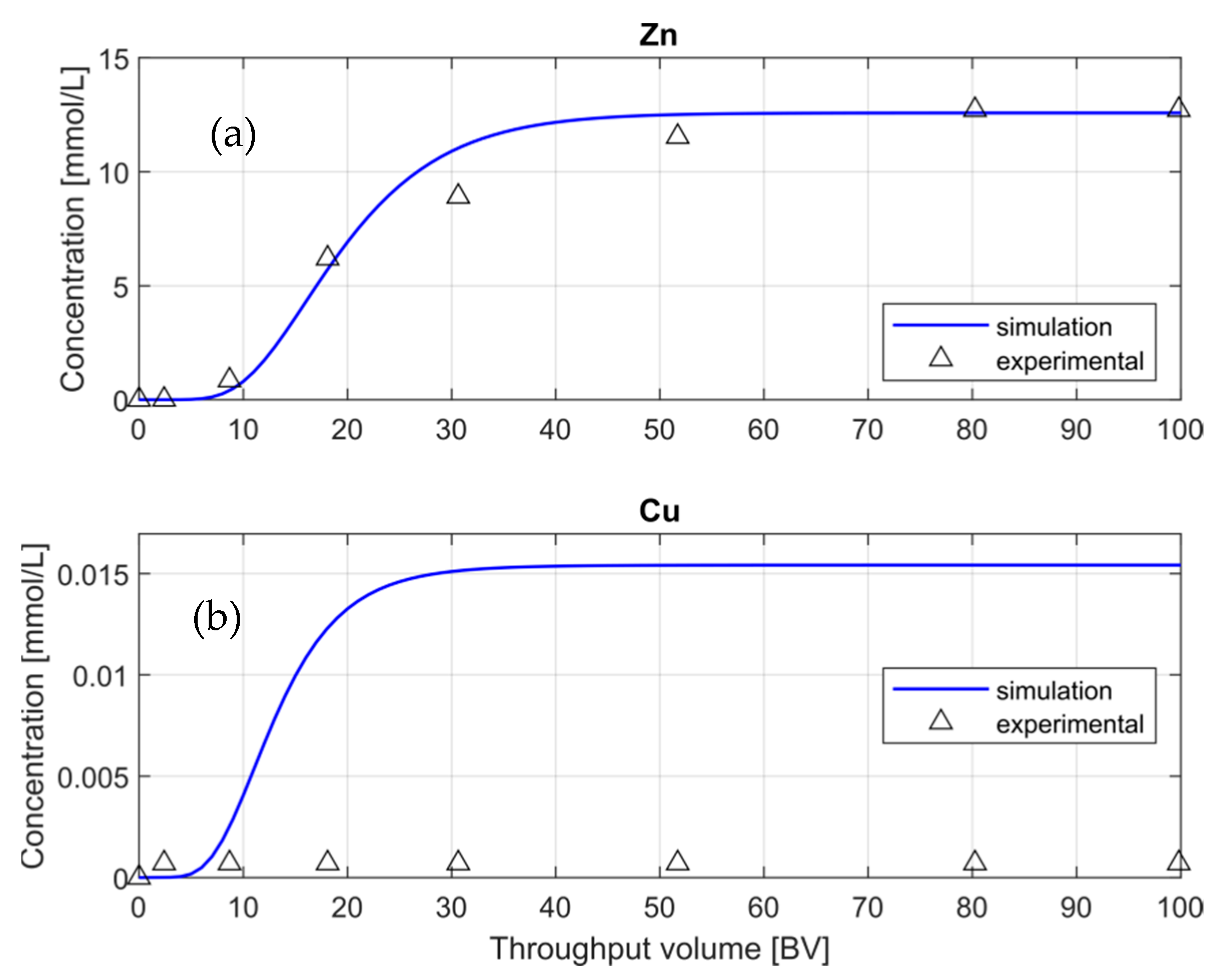
The first model approach was built using Scenario 1. For the first CEC approximation, a value of 48% of water retention was assumed, which is the lowest value from the theoretical rank provided by the manufacturer (Table 2). For the first attempt, default values of exchange and activity coefficients from the phreeqc.dat database were used (see Table 6). Thus, it was not necessary to add extra data in the input file. The simulation and experimental BTCs for Zn+2 and Cu+2 are shown in Figure 4.
As shown in Figure 4a, the Zn-BTC simulation shows similar behavior to the experimental data, mainly at the breakthrough point (BTP) and at the exhaustion stage. On the other hand, Figure 4b shows that the simulation of Cu-BTC does not fit with the experimental data along with the whole pattern. The experimental concentrations of copper were below the detection limit of the MP-AES and never reached the BTP during the loading phase due to its high affinity with the resin TP-220 and its very low concentration in the inflow solution. In any case, Figure 4 shows that the simulated Zn+2 and Cu+2-ions have the BTP at nine and five-bed volumes, respectively.
3.2. Sensitivity Analysis of Parameters and Coefficients
A sensitivity analysis was performed for Scenario 1 in order to identify the main parameters and coefficients that govern the model. As mentioned above, the parameters identified as having the greatest impact on the IX process are CEC, selectivity coefficients, activity coefficients, pH, and flow rate. Although the pH and flow rate have a significant impact on the model, these parameters have values established during the experimental tests that will be taken for the input definition. Therefore, the behavior of the breakthrough curves at different CEC, exchange coefficients, and activity coefficients are shown in Figure 5, Figure 6 and Figure 7.
3.2.1. Cation Exchange Capacity
Since the theoretical capacity of the exchanger is not a defined parameter because it depends on the effective porosity, water retention of the resin, and operating conditions, it is necessary to evaluate it [29]. For this purpose, Figure 5 shows different CEC values in mol/Lw (mol per liter of water) that were set to evaluate their impact on the model. This range of values was estimated by defining different water retention percentages of the resin based on the results of the first model approach.
Due to the significant difference between the output concentrations of Zn+2 and Cu+2, separate graphs were plotted for a more detailed assessment of the trends. The behavior of Zn- and Cu-BTCs in Figure 5 are affected following the same pattern. The higher the CEC, the later the BTP, observing a difference of 10-BV between the BTP calculated at the lowest (0.246) and highest (1.065) CEC. It can be seen in both cases a flatter slope for the highest CEC value selected. Due to the high impact of this parameter on the model, this variable will be part of the model calibration.
3.2.2. Exchange Coefficients
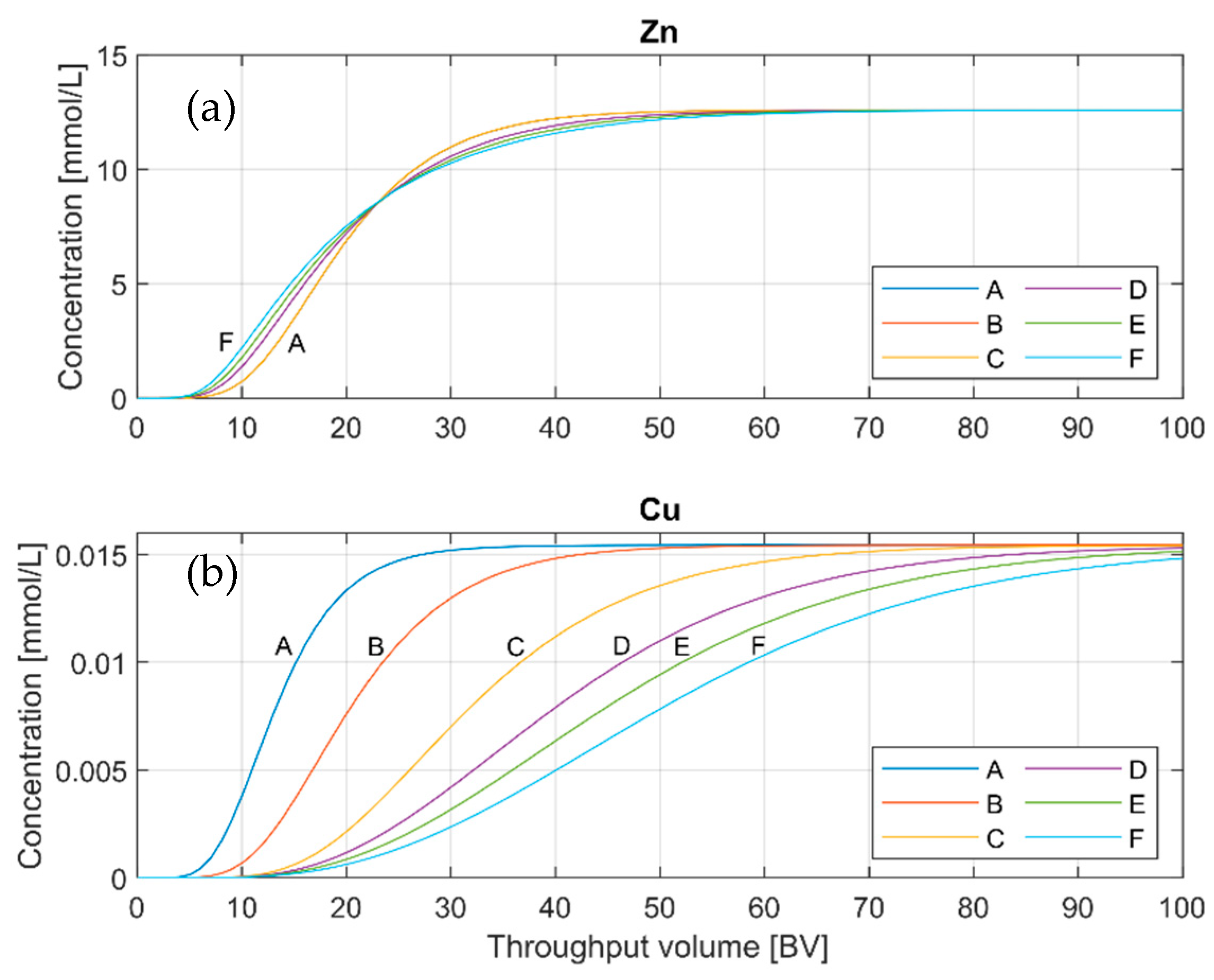
Scenario 1 is a two-cation system, and therefore, it is required to define two exchange coefficients, one for each ion. In order to evaluate the behavior of the BTCs at different exchange coefficient values, different configurations were stated as is described in Table 4. Configuration A describes the values of the exchange coefficients defined by default in the PhreeqC database, and from these starting values, the other configurations were defined: first, increasing the values for the Cu ion and defining a constant value for the Zn ion (Configurations A–C); then, defining a constant value for the Cu ion and decreasing the value for the Zn ion (Configurations C–F). These configurations helped to evaluate the impact and interdependence of exchange coefficients on both metal ions.
Cu-BTCs show a high sensitivity for all the configurations due to its high affinity toward the resin [21,23]. This behavior is stated as Figure 6b shows a distinct trend for each configuration. Analyzing the pattern illustrated in Figure 6b, the following must be pointed out: (1) the higher the Cu coefficient, the flatter the slope and the later the Cu-BTC; (2) the higher the Zn coefficient, the sooner the Cu-BTP. It is observed that there is a difference of 10 BV approximately between the BTP at configuration A and F for the Cu+2 ion.
On the other hand, Figure 6a shows that Zn curve is only affected by its own exchange coefficient (configurations C to F) and follows the same trends as the Cu+2 ion but to a minor degree. In this case, only a difference in the BTPs of 2 BV is visualized for all configurations.
3.2.3. Ion Specific Parameters–Activity Coefficients
Although the parameters a and b are part of the database, an assessment of their behavior under variations will provide information in case further adjustment is required. For example, the default ion-specific parameters b has a value of 0.0 for Cu+2 and Zn+2 ions, while the parameter a presents a different value for each element. Therefore, in order to reduce the number of unknowns, a value of zero will be defined for parameter b for all simulations, while parameter a will be evaluated by setting different values, as shown in Table 5.
Starting with default values, Table 5 describes the different configurations applied to evaluate the impact of activity coefficients. Figure 6 shows the Zn- and Cu-BTCs under configurations A to J.
Figure 7b was plotted using areas (G-J), (F-B) due to the slight variations between one BTC and the other. The trends of the BTCs constitute the areas that curiously fit in the different configurations defined in Table 5 for Cu+2. The behavior shows that at a constant a-parameter for Zn+2, the trend of Cu curves follows: the lower the value of Cu-a, the flatter the slope of the curve. Moreover, at a constant a parameter for Cu+2, the lower the Zn-a, the steeper the slope of the curve. During all the proposed configurations, variations in the slope of the curves can be observed; however, the breakthrough and exhaustion points remain without significant modifications.
The Zn ion once again shows no dependence under Cu-a variations and no significant changes for different Zn-a values. There can be clearly observed in Figure 7a a thick BTC where the impact of the different configurations cannot be visualized due to the low sensitivity.
3.3. Estimation of CEC and Exchange Coefficients
After identifying the key parameters through sensitivity analysis, two of them, CEC and exchange coefficients, were selected for the model calibration based on their high impact on the model. The calibration consists of comparing model and experimental results by adjusting the key parameters until the simulation results match the experimental data [28].
Calibration was performed manually by trial and error. As this is complicated when many parameters and variables are involved, the calibration was performed in two stages: first, a calibration of CEC using default exchange coefficients; then, the calibration of exchange coefficients using the estimated CEC.
The first calibration was performed using Scenario 1 in order to estimate the CEC value and the coefficients for zinc and copper ions. Then, a second calibration was conducted for Scenario 2 using the estimated values from the first calibration and estimating the values for the new metal ions nickel and cobalt. Results can be observed in Figure 8 and Figure 9 where a good approximation for both scenarios is visible.
Figure 8a shows a complete match between the simulation and the experimental data of the Zn-BTC. Then, the Zn-exchange coefficient value is fixed to 0.55. On the other hand, in the case of the Cu+2 ion, as shown in Figure 8b, the experimental data points to compare with are set as 7e−4 [mmol/L]. This value was defined as the limit of detection (LOD) of the MP-AES for the quantification of the Cu+2 ion concentration. Then, a value for the Cu-exchange coefficient must be at least 1.5 to meet this upper limit condition. A lower value would surpass this limit, and a higher one would flatten out the curve. It is important to take in mind that a variation of the Cu-exchange coefficient does not affect the behavior of the Zn curves, as it was shown in Section 3.2.2. Then, the Cu coefficient could be adjusted further, without changing the trend of Zn-BTC.
For the second calibration applying Scenario 2, the Zn-coefficient was not adjusted, since the value of 0.55 was estimated in the first calibration. In the case of the Cu-exchange coefficient from Scenario 1, the value of 1.5 was the minimum starting value for Scenario 2. Therefore, there are three variables for the second model calibration: Co-, Ni-, and Cu-exchange coefficients. Although the Zn ion was not adjusted in this scenario, its trend has to be monitored as well.
The results of the second calibration are shown in Figure 9, where is clearly seen that the calculated BTCs follow the selectivity order of adsorption determined experimentally (Cu+2 > Ni+2 > Co+2 > Zn+2) presented in Table 2. There are no default coefficients for Co+2 and Ni+2 ions in the database. Thus, these coefficients were fit between the most (Cu+2) and the least (Zn+2) affine ions, as is described in Table 6 (Second approach).
In order to show the significant variation that exists in the model when modifying the exchange coefficients, and the possibility to manipulate them, Figure 9 shows the BTCs before and after the calibration of Scenario 2. As a result of the interdependence between ions, the manipulation of one coefficient affects all competing ions in the system. This condition is observed in the estimated Zn and Co curves where the values of their coefficients were kept constant but, nevertheless, they deviate from the experimental data in the range 3 > BV > 5. However, for these two ions, Zn+2 and Co+2, a good calibration of the model is observed. In the case of the Cu+2 and Ni+2 ions, a considerable approximation of the BTCs with the experimental data was achieved. While it is possible to further increase the values of these coefficients to achieve better results, this manipulation would decalibrate the already calibrated ions. Table 6 summarizes the various default and estimated CEC and exchange coefficients over the calibrations performed.
3.4. Model Predictability for a Complex Mine Water Matrix
For the validation of the model, Scenario 3 with a six-cation composition inlet solution as described in Table 1 was predicted. Once the BTCs were obtained, the column was set up to obtain the experimental results. As mentioned previously, the comparison of simulation and experimental BTCs’ position and shape is used to evaluate the accuracy of the model predictability.
The behavior of the BTCs shows a very low resin affinity of all ions but Cu+2. That is why the BTPs of the cations were reached before the 5-BV was injected. In order to assess in more detail the predicted and experimental BTC, Figure 10 shows a closer view of each ion separately.
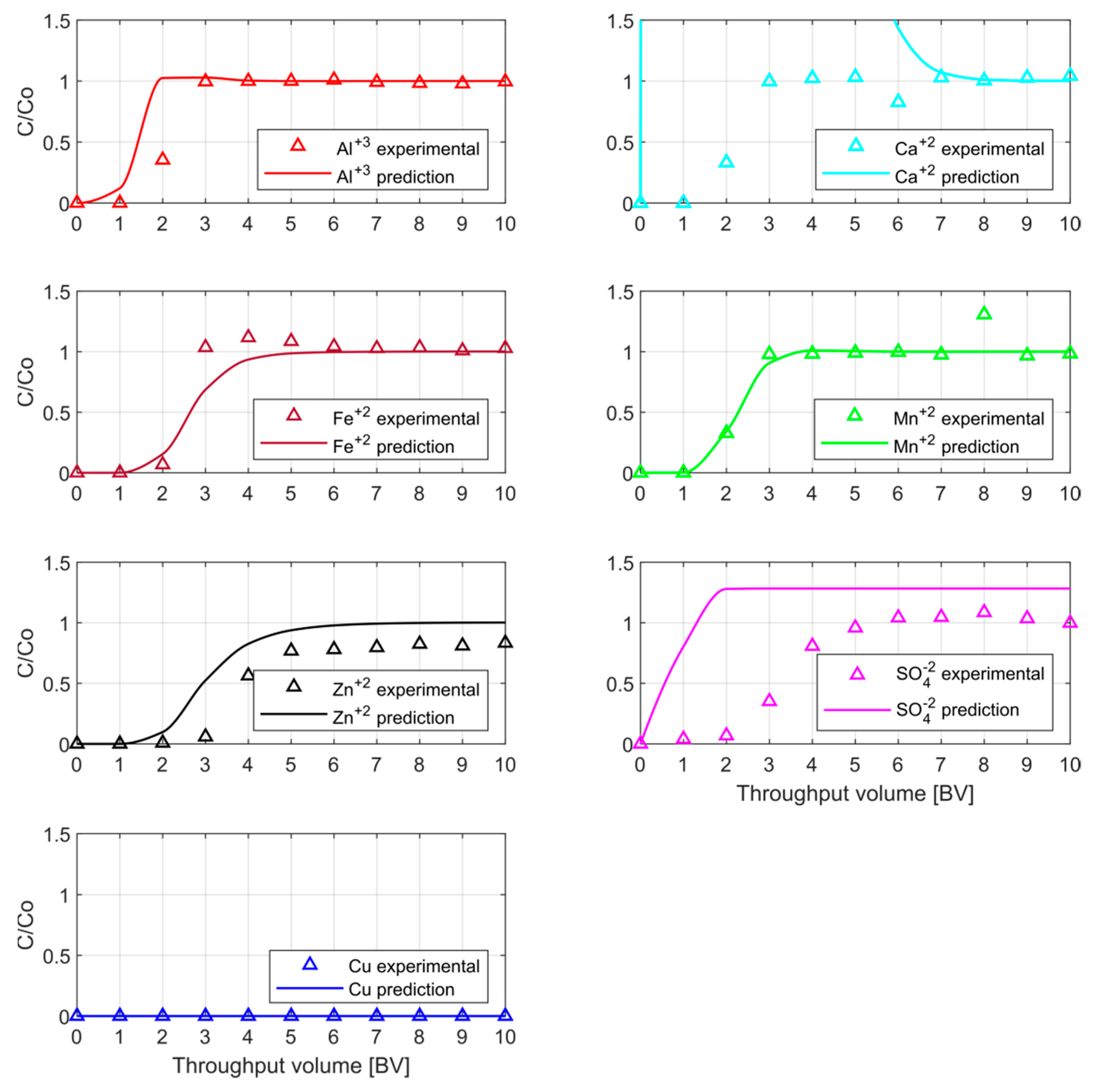
In this second part of the research, not only metal ions but also sulfate and calcium ions were evaluated in order to make a deeper evaluation of the model under more real conditions. From Figure 10, it can be observed that for the only anion considered, SO4−2, there is no match between predicted and experimental data. The predicted curve has a sharp increase in concentration from the beginning of the loading phase, while the experimental one has a sigmoidal-shaped curve with a BTP at one BV. On the other hand, the alkali earth metal, Ca+2 that was part of the inflow solution, matches only from the 7-BV onwards, having an overestimated concentration in the predicted curve. Experimental BTCs also show a sigmoidal-shaped behavior until they reach maximum concentration at 3-BV.
In the case of Al+3, the shapes of predicted and experimental curves are similar. The predicted BTP is slightly earlier than the experimental one, but there is a complete match from 3-BV onwards. The predicted Mn+2 -BTC overlaps the experimental one, showing a good approximation. It can be seen as an auspicious outcome for Fe+2, matching both curves along with the pattern. The metal ion Zn+2 shows a similar sigmoidal shape between predictions and experimental BTCs. Nevertheless, the predicted BTP takes place 1-BV earlier than the experimental one. Finally, for Cu+2, the most resin-affine ion, the graph shows no presence of this cation in the outflow solution during the experimental loading, and this characteristic was also predicted.
4. Discussion
4.1. Identification of Major Model Parameters
The first model approach revealed that the model requires an adjustment of parameters, since the simulation and experimental Cu+2-BTCs do not match. Therefore, three parameters governing the model were identified through the sensitivity analysis: CEC, exchange coefficients, and activity coefficients (function of ion-specific parameters a and b). The behavior of the BTCs under variations of the key parameters was presented in Figure 5, Figure 6 and Figure 7. Based on this analysis, the main findings regarding the studied parameters are described below and were later applied for the characterization and calibration of the model.
CEC: This parameter showed the highest impact on the model. The behavior of the curves shown in Figure 5 follows the theoretical background that the higher the CEC, the higher the number of exchange sites in the resin and hence a later BTP [12,39]. However, it is essential to note that minor variations in the value of this parameter significantly affect the behavior of the IX process so that its estimation and definition are accurate. Synthetic resins are characterized by their high capacity; however, an erroneous definition of their real value significantly reduces or increases their performance.
Exchange coefficients: Exchange coefficients represent the selectivity or affinity rank of the ions toward the exchanger. Then, the definition of one coefficient affects the behavior of the rest of the competing ions in the system, especially for ions with high affinity toward the resin. In this study, Cu+2 has the highest exchange coefficient and is therefore the most sensitive cation in the system, as shown during the sensitivity analysis (Figure 6).
Scenario 1 presents two cations, Cu+2 and Zn+2. Thus, it was necessary to define two exchange coefficients: one for each competing cation. As a result, for all configurations described in Table 4, there are significant effects in the results showing interdependence between the ions that make up the system. This is why complex matrices are more challenging to simulate, as they have a greater number of ions and therefore present a greater number of unknowns.
Activity coefficients: The sensitivity analysis of activity coefficients (function of ion specific parameters a, b) showed that this parameter affects only the most affine element copper. However, the impact of this parameter is not as significant as the CEC and the exchange coefficients. The behavior that follows the most affine ion in the analysis of Scenario 1 is, the lower the value of the a coefficient, the later the BTP. This effect is due to a coefficients being related to the activity of exchange species, affecting directly their concentration [15,26].
Given the lower impact of this parameter in the model and in order to reduce the number of unknowns to be estimated through the calibration process, the study was continued using theoretical values defined in the phreeqc.dat database. During the simulation of Scenario 2, where Ni+2 and Co+2 ions are present, it was required to define their coefficients because they are not included in the database. To calculate the activity coefficients of these two metals, the ion-specific-parameter a was assumed as 6.0 and 5.0 for Ni+2 and Co+2, respectively, based on default values for divalent elements [15]. It must be noticed that if ion-specific parameters are not defined whether in the input file or as part of the database, the activity of the exchange specie is equal to its equivalent fraction as in ideal behaviors [12].
4.2. Model Calibration
The key parameters are interrelated, and therefore, the calibration of a parameter may deteriorate the calibration of a previous or later stage [28,38]. To overcome this condition, the calibrations were repeated iteratively following the proposed methodology of starting the coefficient estimation with a two-cation system followed by a four-cation system [38].
The first parameter estimated was the CEC with a value of 0.617 (mol/Lw), and it was used for all scenarios. This value was calculated after the assessment of the parameter by sensitivity analysis and later calibration with experimental data from Scenario 1. The theoretical CEC proposed by the manufacturer establishes a range of 0.304–0.494 (mol/Lw); however, the estimated value exceeds the upper limit by nearly 25%. This difference is significant for the process and verifies that the theoretical CEC should be evaluated according to the particularities of each case study. The initial composition of the cation exchanger was defined implicitly in the model, stating that the exchanger is in equilibrium with an initial solution of known composition, which was analyzed in the laboratory. For further study, the definition of the initial capacity can be done by injecting a tracer as the inflow solution in a column test, and later, by defining the exchange assemblage explicitly in the input file listing the composition of each exchange component [15].
The approach of using experimental selectivity ranks as a guide to define the exchange coefficient values was helpful given the number of unknowns. Once the exchange coefficients of Zn+2 and Cu+2 were estimated in Scenario 1, these values were used to define the upper and lower limits for Scenario 2 and fit the Co- and Ni-exchange coefficients between the most (Cu+2) and the least (Zn+2) affine ion. The same criterion was used for the definition of exchange coefficients for Scenario 3. Then, it is shown in Figure 8 and Figure 9 that the order of appearance of the BTCs corresponds to the value of the coefficient assigned for each element. The lower the exchange coefficient, the lower the affinity toward the resin [40].
Table 6 describes estimated values of the eight exchange coefficients of which six have default values as part of the selected database [15]. By calculating the percentage difference between estimated and default values, we obtain Cu+2(+483%), Zn+2(−31%), Fe+2(−20%), Mn+2(−60%), Al+3(−51%), and Ca+2(−76%). The high Cu+2 selectivity of the resin studied is reflected in two aspects, the first showing that the estimated coefficient for the Cu+2 ion is far above the default value, and secondly, that the reduction of the coefficients of the rest of the cations is more than 20%. These results confirm that the exchange coefficients present in the software database that were estimated from natural materials need to be adjusted when modeling synthetic resins with such specific selectivities and properties [41]. On the other hand, there is a lack of theoretical coefficients and kinetic data for some species. Thus, it was required to define thermodynamic parameters for Ni+2 and Co+2, assuming only primary master species for both metals during their definition in the input file.
The values estimated in this study can be taken as a reference point specifically for IX columns filled with Lewatit® MonoPlus TP-220 resin. It is worth noting that the parameters estimated in Table 6 are by no means constant.
4.3. Validation of Model Predictability for a Complex Mine Water
The purpose of this study was to develop a model that can be applied for the prediction of the adsorption process of IX columns using as an inflow complex mine water matrices. Thus, it is important to highlight that the validation experiment was performed using as input solution a six-cation system (Scenario 3) containing Al+3, Mn+2, Ca+2, and sulfate ions, which were not studied previously during the parameter estimation.
For a first evaluation of the model predictability, a comparison between predicted and experimental selectivity ranks was made, as described in Table 7. It is understood that the predicted selectivity rank for Scenario 3 shows a differentiated rank of all the cations, with Cu+2 as the most affine and Ca+2 the least. On the other hand, the experimental rank for this scenario shows a similar order to its prediction. However, for Mn+2, Al+3, and Ca+2, it was not possible to differentiate the rank of BTPs, since the concentration of these ions was present in the outflow from the first BV due to the lack of affinity toward the resin.
A second assessment for the model validation is a comparison of the position and shape between predicted and experimental BTCs. Figure 10 illustrates the BTCs of the ions involved in the multi-ion system. The calculated BTCs for all the metal ions have a relatively good shape approximation to the experimental ones with the values of CEC and exchange coefficients described in Table 6. However, a small discrepancy is observed in the Al+3-BTP, where the prediction curve is 0.5 BV ahead of the experimental curve, but both have the same shape during the run. In the case of Zn+2, the curve prediction indicates breakthrough and exhaustion points that are ahead of the experimental data. These discrepancies are probably due to the significant difference between the Scenario 2 and Scenario 3 inflow concentrations of more than 100 times in the case of Cu+2. As mentioned above, the ions sorption is affected by the presence of competing ions [26].
There is an overestimation of Ca+2 and sulfates in the region 0 < BV < 7 and 0 < BV < 10, respectively. The sulfates mismatch may be related to gypsum equilibrium and its precipitation/dissolution inside the column. The behavior of gypsum is closely affected by Ca+2 concentrations and therefore related to the IX reactions and the definition of exchange coefficients [29]. The steep increase of Ca+2 concentration at the beginning of the prediction is possibly due to the implicit definition of the initial exchanger composition obtained by batch experiments where Ca+2 was present. Nevertheless, in order to acquire a better understanding of the phenomena, further research is planned to investigate the used resin through SIMS analysis.
The variation of exchange coefficients and the neglect of other reactions and processes that can take place during the adsorption process can lead to the differences observed between experimental and simulation results [40]. Therefore, the determination of the exchange coefficients was performed by fitting their values with experimental results, since the default values of the databases do not match the dynamic system of experimental columns and the peculiarities of the synthetic exchanger material [41]. This methodology allows the approximation of real cases with complex matrices but also shows us that the definition of specific properties is required for optimal results.
5. Conclusions
A 1D reactive transport model based on PhreeqC code has been developed to simulate the selective removal of metals from acidic mine waters by chelating bis-picolylamine resins (Lewatit® MonoPlus TP-220). The BTCs obtained through simulations helped to identify and study the three key parameters that can govern the adsorption model: CEC, exchange coefficients, and activity coefficients. The model was used to simulate systems with two-cation, four-cation, and six-cation inflow compositions. This configuration of scenarios helped gradually evaluate and upgrade the model while estimating values for CEC and exchange coefficients. The significant percentage difference determined between the theoretical and estimated values confirms, firstly, that the default exchange coefficients require adjustment when using synthetic resins. In addition, the theoretical CEC of the exchanger should be experimentally verified according to the characteristics of each case. For the particularities and boundary conditions proposed in this study, the estimated values are considered stochastic variables.
This study took a novel approach to model IX processes with complex mine water matrices. We obtained good correlations and were able to improve the results through iterative calibrations.
This first approach presents deviations in some components of the proposed systems and does not take into account other possible reactions that may be part of the process. However, these deficiencies can be overcome with further iterative calibration and post-use resin studies. Due to the great potential of the process and synthetic resins, this methodology is proposed, as it allows results to be obtained in very short periods of time and at low or no cost.
To improve the knowledge, we want to strengthen this research with microscopic analysis of the exchanger material to evaluate other types of reactions that may occur and affect the IX process and incorporate the UCODE program to estimate more parameters that can further boost the model’s scope. Once the upgraded model is established, it could be used to model IX processes for all kind of real scenarios.
Author Contributions
Investigation, Simulation, Writing—original draft preparation, Formal analysis, Writing—review and editing, A.I.P.M.; Conceptualization, Methodology, Supervision, Visualization, Writing—review and editing, J.A.; Conceptualization, Supervision, Validation, Writing—review and editing, N.H.; Sample analysis, Visualization, Writing—review and editing, M.G.; Funding acquisition, Validation, Writing—review and editing, C.D. All authors have read and agreed to the published version of the manuscript.
Funding
This research has been done as a part of the SECMINTEC project (support code 022R186A) funded by the Federal Ministry of Education and Research in Germany (BMBF) inside the CLIENT program.
Institutional Review Board Statement
Not applicable.
Informed Consent Statement
Not applicable.
Data Availability Statement
The data presented in this study are available on request from the corresponding author. The data are not publicly available due to privacy.
Acknowledgments
The authors would like to acknowledge Lanxess Deutschland GmbH for providing the resin samples. We also want to thank for the cooperation of Sandra Teruya, David Farfán and Ozan Aydin for helping in laboratory experiments. The support of Viktoria Mezovská for the handling and analysis of samples is also gratefully acknowledged.
Conflicts of Interest
The authors declare no conflict of interest.
References
- Johnson, D.B.; Hallberg, K.B. Acid mine drainage remediation options: A review. Sci. Total Environ. 2005, 338, 3–14. [Google Scholar] [CrossRef]
- Park, S.-M.; Yoo, J.-C.; Ji, S.-W.; Yang, J.-S.; Baek, K. Selective recovery of dissolved Fe, Al, Cu, and Zn in acid mine drainage based on modeling to predict precipitation pH. Environ. Sci. Pollut. Res. 2015, 22, 3013–3022. [Google Scholar] [CrossRef]
- Naidu, G.; Ryu, S.; Thiruvenkatachari, R.; Choi, Y.; Jeong, S.; Vigneswaran, S. A critical review on remediation, reuse, and resource recovery from acid mine drainage. Environ. Pollut. 2019, 247, 1110–1124. [Google Scholar] [CrossRef] [PubMed]
- Neumann, S.; Fatula, P. Principles of ion exchange in wastewater treatment. Asian Water 2009, 19, 14–19. [Google Scholar]
- Inamuddin, M. (Ed.) Ion Exchange Technology I: Theory and Materials; Springer: Berlin/Heidelberg, Germany, 2012. [Google Scholar]
- Kumar, P.; Pournara, A.; Kim, K.-H.; Bansal, V.; Rapti, S.; Manos, M.J. Metal-organic frameworks: Challenges and opportunities for ion-exchange/sorption applications. Prog. Mater. Sci. 2017, 86, 25–74. [Google Scholar] [CrossRef]
- Alguacil, F.J.; Alonso, M.; Lozano, L.J. Chromium (III) recovery from waste acid solution by ion exchange processing using Amberlite IR-120 resin: Batch and continuous ion exchange modelling. Chemosphere 2004, 57, 789–793. [Google Scholar] [CrossRef] [PubMed]
- Oyewo, O.A.; Agboola, O.; Onyango, M.S.; Popoola, P.; Bobape, M.F. Current methods for the remediation of acid mine drainage including continuous removal of metals from wastewater and mine dump. In Bio-Geotechnologies for Mine Site Rehabilitation; Elsevier: Amsterdam, The Netherlands, 2018; pp. 103–114. ISBN 9780128129869. [Google Scholar]
- Botelho Junior, A.B.; Vicente, A.d.A.; Espinosa, D.C.R.; Tenório, J.A.S. Recovery of metals by ion exchange process using chelating resin and sodium dithionite. J. Mater. Res. Technol. 2019, 8, 4464–4469. [Google Scholar] [CrossRef]
- Karlsson, D.; Jakobsson, N.; Brink, K.-J.; Axelsson, A.; Nilsson, B. Methodologies for model calibration to assist the design of a preparative ion-exchange step for antibody purification. J. Chromatogr. A 2004, 1033, 71–82. [Google Scholar] [CrossRef] [PubMed]
- Yılmaz İpek, İ.; Kabay, N.; Yüksel, M. Modeling of fixed bed column studies for removal of boron from geothermal water by selective chelating ion exchange resins. Desalination 2013, 310, 151–157. [Google Scholar] [CrossRef]
- Merkel, B.; Planer-Friedrich, B.; Nordstrom, D.K. Groundwater Geochemistry: A Practical Guide to Modeling of Natural and Contaminated Aquatic Systems, 2nd ed.; Springer: Berlin/Heidelberg, Germany, 2008; ISBN 9783540746676. [Google Scholar]
- Camden-Smith, B.; Johnson, R.H.; Camden-Smith, P.; Tutu, H. Geochemical modelling of water quality and solutes transport from mining environments. In Research and Practices in Water Quality; Lee, T.S., Ed.; InTech: London, UK, 2015; ISBN 978-953-51-2163-3. [Google Scholar]
- Franken, G.; Postma, D.; Duijnisveld, W.H.; Böttcher, J.; Molson, J. Acid groundwater in an anoxic aquifer: Reactive transport modelling of buffering processes. Appl. Geochem. 2009, 24, 890–899. [Google Scholar] [CrossRef]
- Parkhurst, D.L.; Appelo, C.A. Description of Input and Examples for Phreeqc Version 3—A Computer Program for Speciation, Batch-Reaction, One-Dimensional Transport, and Inverse Geochemical Calculations, 6th ed.; U:S: Geological Survey Techniques and Methods; U.S. Geological Survey: Reston, VA, USA, 2013. Available online: http://pubs.usgs.gov/tm/06/a43/ (accessed on 28 September 2021).
- Tertre, E.; Beaucaire, C.; Coreau, N.; Juery, A. Modelling Zn(II) sorption onto clayey sediments using a multi-site ion-exchange model. Appl. Geochem. 2009, 24, 1852–1861. [Google Scholar] [CrossRef] [Green Version]
- Alguacil, F.J.; Garcia-Diaz, I.; Lopez, F. The removal of chromium (III) from aqueous solution by ion exchange on Amberlite 200 resin: Batch and continuous ion exchange modelling. Desalination Water Treat. 2012, 45, 55–60. [Google Scholar] [CrossRef]
- Lin, S.H.; Kiang, C.D. Chromic acid recovery from waste acid solution by an ion exchange process: Equilibrium and column ion exchange modeling. Chem. Eng. J. 2003, 92, 193–199. [Google Scholar] [CrossRef]
- Dabrowski, A.; Hubicki, Z.; Podkościelny, P.; Robens, E. Selective removal of the heavy metal ions from waters and industrial wastewaters by ion-exchange method. Chemosphere 2004, 56, 91–106. [Google Scholar] [CrossRef] [PubMed]
- Shaidan, N.H.; Eldemerdash, U.; Awad, S. Removal of Ni(II) ions from aqueous solutions using fixed-bed ion exchange column technique. J. Taiwan Inst. Chem. Eng. 2012, 43, 40–45. [Google Scholar] [CrossRef]
- Wołowicz, A.; Hubicki, Z. Enhanced removal of copper(II) from acidic streams using functional resins: Batch and column studies. J. Mater. Sci. 2020, 55, 13687–13715. [Google Scholar] [CrossRef]
- Wołowicz, A.; Hubicki, Z. The use of the chelating resin of a new generation Lewatit MonoPlus TP-220 with the bis-picolylamine functional groups in the removal of selected metal ions from acidic solutions. Chem. Eng. J. 2012, 197, 493–508. [Google Scholar] [CrossRef]
- Lanxess Energizing Chemistry. Product Information Lewatit MonoPlus TP 220 [Fact sheet]. 2020. [Google Scholar]
- Wołowicz, A. Zinc(II) removal from model chloride and chloride–nitrate(V) Solutions using various sorbents. Physicochem. Probl. Miner. Process. 2019, 55, 1517–1534. [Google Scholar] [CrossRef]
- Kołodyńska, D.; Sofińska-Chmiel, W.; Mendyk, E.; Hubicki, Z. DOWEX M 4195 and LEWATIT ® MonoPlus TP 220 in Heavy Metal Ions Removal from Acidic Streams. Sep. Sci. Technol. 2014, 49, 2003–2015. [Google Scholar] [CrossRef]
- Appelo, C.; Postma, D. Geochemistry, Groundwater and Pollution; CRC Press: Boca Raton, FL, USA, 2004; ISBN 9780429152320. [Google Scholar]
- Appelo, C.; Verweij, E.; Schäfer, H. A hydrogeochemical transport model for an oxidation experiment with pyrite/calcite/exchangers/organic matter containing sand. Appl. Geochem. 1998, 13, 257–268. [Google Scholar] [CrossRef]
- Saaltink, M.W.; Ayora, C.; Stuyfzand, P.J.; Timmer, H. Analysis of a deep well recharge experiment by calibrating a reactive transport model with field data. J. Contam. Hydrol. 2003, 65, 1–18. [Google Scholar] [CrossRef]
- Boluda-Botella, N.; Valdes-Abellan, J.; Pedraza, R. Applying reactive models to column experiments to assess the hydrogeochemistry of seawater intrusion: Optimising ACUAINTRUSION and selecting cation exchange coefficients with PHREEQC. J. Hydrol. 2014, 510, 59–69. [Google Scholar] [CrossRef]
- Kyllönen, J.; Hakanen, M.; Lindberg, A.; Harjula, R.; Vehkamäki, M.; Lehto, J. Modeling of cesium sorption on biotite using cation exchange selectivity coefficients. Radiochim. Acta 2014, 102, 919–929. [Google Scholar] [CrossRef]
- Birta, L.G.; Arbez, G. A Conceptual modelling framework for DEDS. In Modelling and Simulation; Springer: London, UK, 2013; pp. 99–168. [Google Scholar]
- Poeter, E.P.; Hill, M.C. UCODE, a computer code for universal inverse modeling. Comput. Geosci. 1999, 25, 457–462. [Google Scholar] [CrossRef]
- Botelho, A.B.; Espinosa, D.C.R.; Dreisinger, D.; Tenório, J.A.S. Effect of PH to recover Cu(ii), Ni(ii) and Co(ii) from nickel laterite leach using chelating resins. Tecnol. Metal. Mater. Min. 2019, 16, 135–140. [Google Scholar] [CrossRef]
- Kang, N.-H.; Park, K.-H.; Parhi, P.K. Recovery of Nickel from sulfuric acid solution using Lewatit TP 220 ion exchange resin. J. Korean Inst. Resour. Recycl. 2011, 20, 28–36. [Google Scholar] [CrossRef] [Green Version]
- Littlejohn, P.; Vaughan, J. Selectivity of commercial and novel mixed functionality cation exchange resins in mildly acidic sulfate and mixed sulfate–chloride solution. Hydrometallurgy 2012, 121, 90–99. [Google Scholar] [CrossRef]
- Malmström, M.E.; Destouni, G.; Martinet, P. Modeling expected solute concentration in randomly heterogeneous flow systems with multicomponent reactions. Environ. Sci. Technol. 2004, 38, 2673–2679. [Google Scholar] [CrossRef] [PubMed]
- Ooi, K.; Makita, Y.; Sonoda, A.; Chitrakar, R.; Tasaki-Handa, Y.; Nakazato, T. Modelling of column lithium adsorption from pH-buffered brine using surface Li+/H+ ion exchange reaction. Chem. Eng. J. 2016, 288, 137–145. [Google Scholar] [CrossRef]
- Robin, V.; Tertre, E.; Beaucaire, C.; Regnault, O.; Descostes, M. Experimental data and assessment of predictive modeling for radium ion-exchange on beidellite, a swelling clay mineral with a tetrahedral charge. Appl. Geochem. 2017, 85, 1–9. [Google Scholar] [CrossRef]
- Robinson, S. Conceptual modelling for simulation Part I: Definition and requirements. J. Oper. Res. Soc. 2008, 59, 278–290. [Google Scholar] [CrossRef] [Green Version]
- Woodberry, P.; Stevens, G.; Northcott, K.; Snape, I.; Stark, S. Field trial of ion-exchange resin columns for removal of metal contaminants, Thala Valley Tip, Casey Station, Antarctica. Cold Reg. Sci. Technol. 2007, 48, 105–117. [Google Scholar] [CrossRef]
- Hörbrand, T.; Baumann, T.; Moog, H.C. Validation of hydrogeochemical databases for problems in deep geothermal energy. Geotherml Energy 2018, 6, 20. [Google Scholar] [CrossRef]
Figure 1.
Flow diagram of the modeling approach.

Figure 2.
Scheme of the experimental IX column system using different inflow solutions for Scenarios 1–3.
Figure 2.
Scheme of the experimental IX column system using different inflow solutions for Scenarios 1–3.
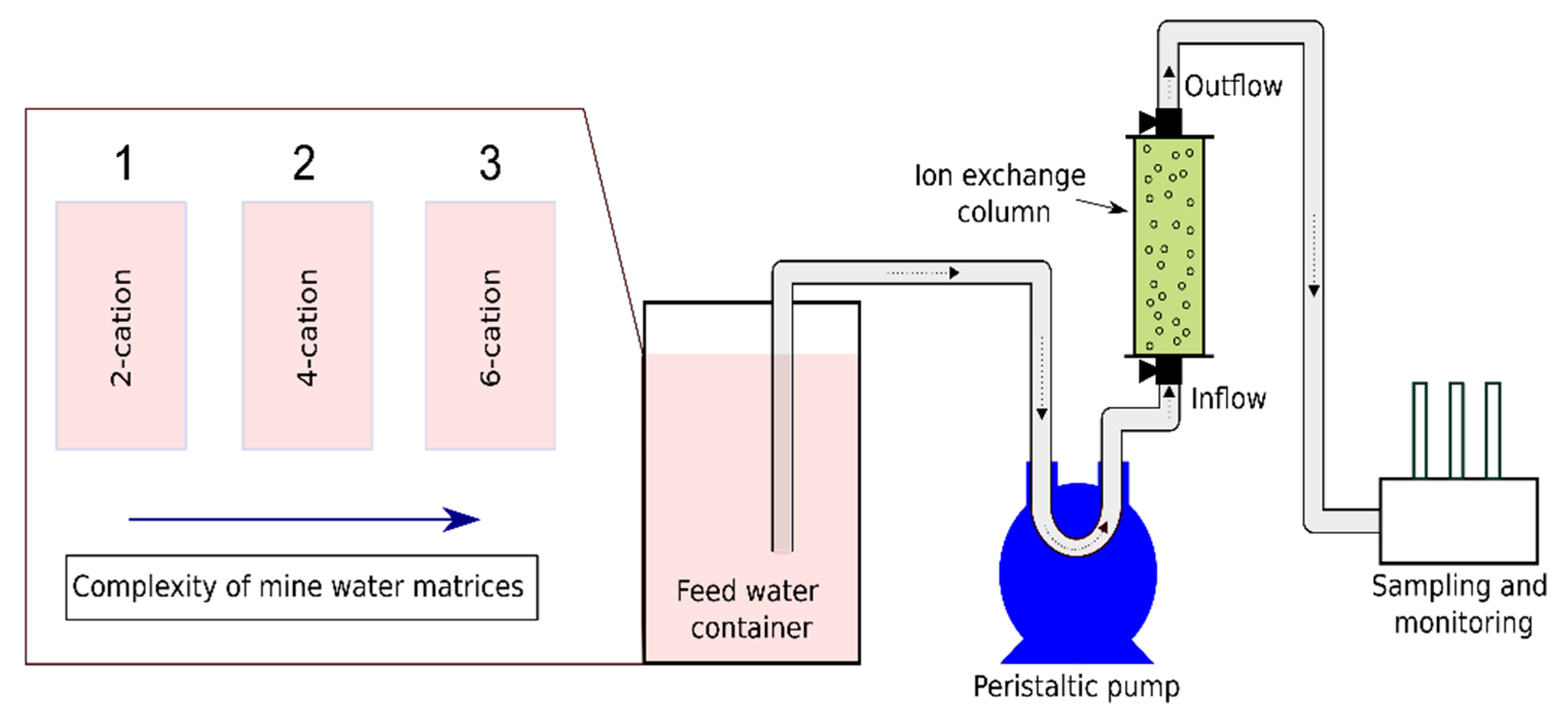
Figure 3.
Conceptual model and column discretization.

Figure 4.
First model approach for Scenario 1. Zn+2 (a), Cu+2 (b); Simulation (solid curves), Experimental (triangles).
Figure 4.
First model approach for Scenario 1. Zn+2 (a), Cu+2 (b); Simulation (solid curves), Experimental (triangles).

Figure 5.
Impact of the CEC value on the model. Zn+2 (a), Cu+2 (b). Scenario 1.
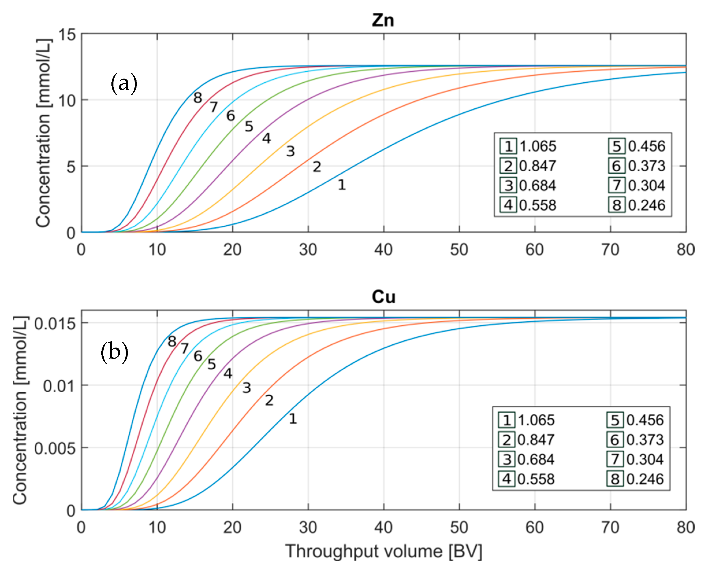
Figure 6.
Impact of the exchange coefficient on the model. Zn+2 (a), Cu+2 (b). Scenario 1.

Figure 7.
Impact of the activity coefficient value on the model. Zn+2 (a), Cu+2 (b). Scenario 1.
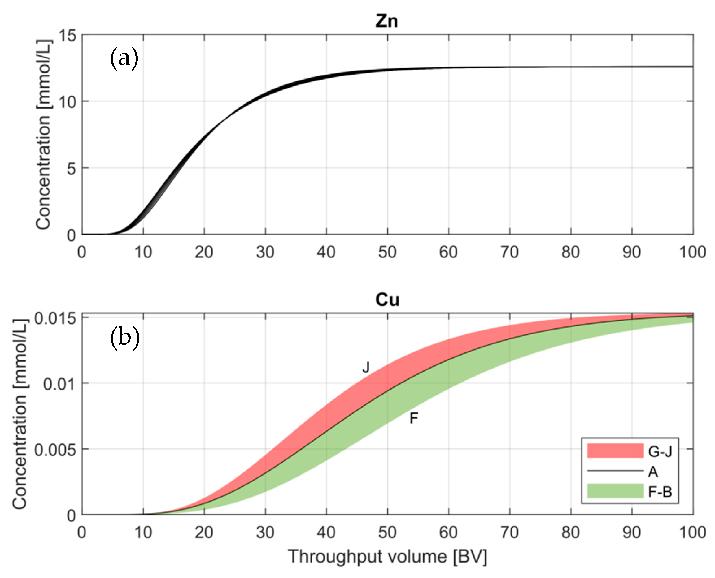
Figure 8.
Model calibration for Scenario 1. Zn+2 (a) and Cu+2 (b). Simulation (solid curve), experimental (triangles).
Figure 8.
Model calibration for Scenario 1. Zn+2 (a) and Cu+2 (b). Simulation (solid curve), experimental (triangles).
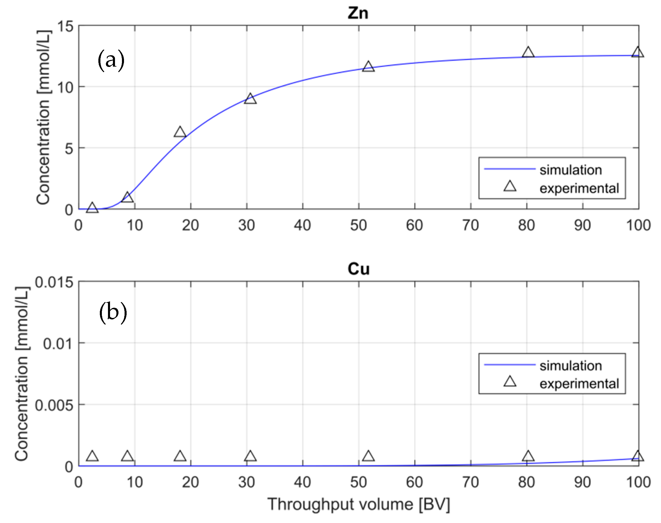
Figure 9.
Model calibration for Scenario 2. Simulation using second approach values (dashed curves), Simulation using estimated values (solid curve), Experimental (triangles).
Figure 9.
Model calibration for Scenario 2. Simulation using second approach values (dashed curves), Simulation using estimated values (solid curve), Experimental (triangles).
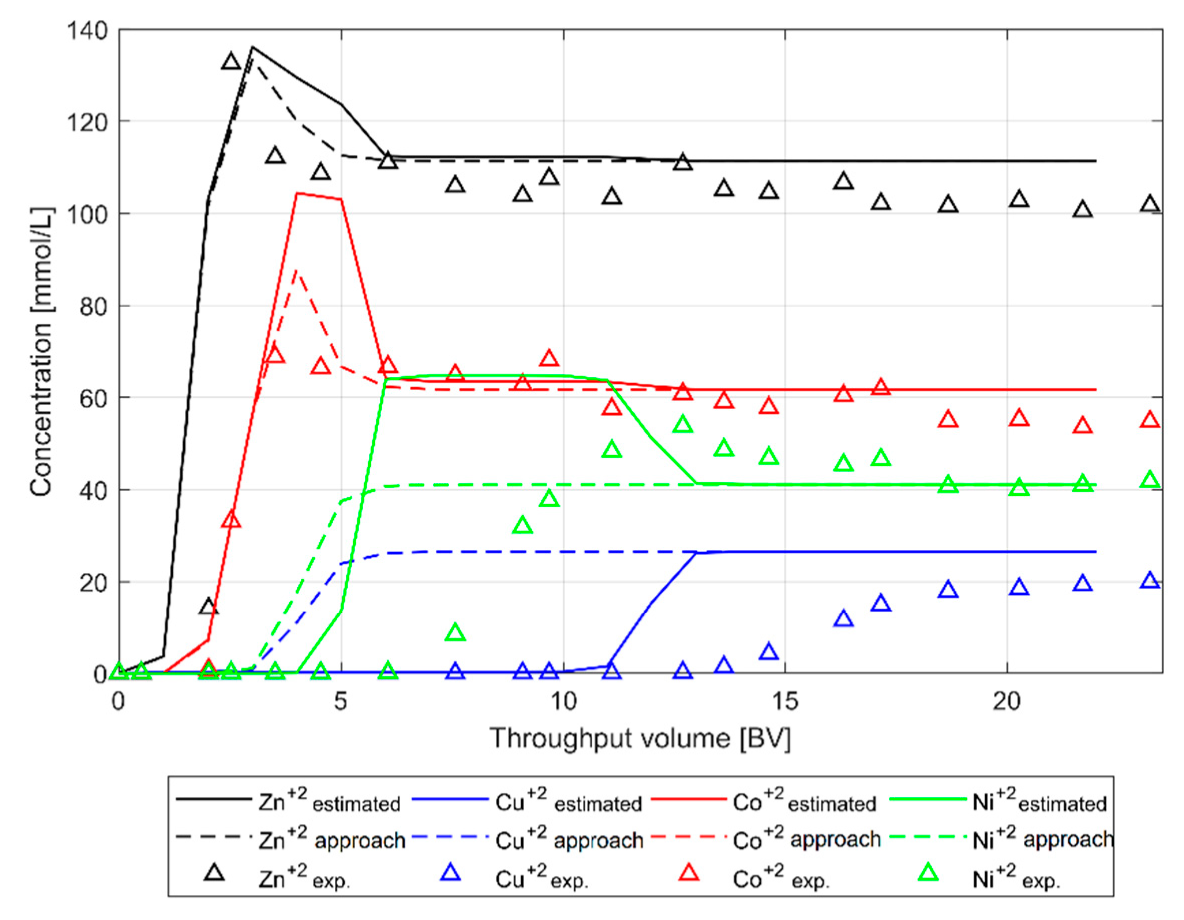
Figure 10.
Assessment for model predictability validation. Solid curves for prediction, triangles for experimental.
Figure 10.
Assessment for model predictability validation. Solid curves for prediction, triangles for experimental.

Table 1.
Characterization of inflow waters for Scenarios 1–3.
| Parameter | Scenario 1 | Scenario 2 | Scenario 3 |
|---|---|---|---|
| Conc. [mg/L] | |||
| pH | 3.27 | 4.66 | 2.5 |
| Al+3 | 236 | ||
| Ca+2 | 20 | ||
| Co+2 | 3637 | ||
| Cu+2 | 0.98 | 1687 | 18 |
| Fe+2 | 2000 | ||
| Mn+2 | 110 | ||
| Ni+2 | 2414 | ||
| Sulfates | 960 | 23,107 | 15,725 |
| Zn+2 | 822 | 7285 | 7000 |
Table 2.
Properties of the resin Lewatit® MonoPlus TP-220 for Scenarios 1–3.
| Scenario | Water Retention 1 | Theoretical CEC 1 | Selectivity Rank |
|---|---|---|---|
| 1 | 0.456 g-Cu/Lresin (min.) | Cu+2 > Zn+2 | |
| 2 | 48–60% | Cu+2 > Ni+2 > Co+2 > Zn+2 | |
| 3 | Cu+2 >> Zn+2 > Fe+2 > Mn+2 > Al+3 > Ca+2 | ||
| Theoretical selectivity Rank 1 (pH = 2): | Cu+2 >> Ni+2 > Fe+3 > Zn+2 > Co+2 > Fe+2 | ||
1 Theoretical data from the manufacturer [23].
Table 3.
Column geometry and hydraulic characteristics for Scenarios 1–3.
| Scenario | Length [m] | Diameter [m] | BV [L] | Inflow Rate [BV/h] | Throughput BV | Total Throughput BV | ||
|---|---|---|---|---|---|---|---|---|
| Day | Night | Day | Night | |||||
| 1 | 0.057 | 0.015 | 0.01 | 6 | 1 | 30;50 | 20 | 100 |
| 2 | 0.120 | 0.040 | 0.15 | 1 | 0.05 | 9 | 14 | 23 |
| 3 | 0.057 | 0.015 | 0.01 | 3 | - | 30 | - | 30 |
Table 4.
Configurations for the exchange coefficients assessment.
| Exchange Coefficients | ||||||
|---|---|---|---|---|---|---|
| A 1 | B | C | D | E | F | |
| Zn+2 | 0.8 | 0.8 | 0.8 | 0.7 | 0.65 | 0.6 |
| Cu+2 | 0.6 | 0.8 | 1.0 | 1.0 | 1.0 | 1.0 |
1 Default coefficient values from phreeqc.dat database.
Table 5.
Configurations for the activity coefficients assessment.
| Ion-Specific Parameter a (b = 0.0) | ||||||||||
|---|---|---|---|---|---|---|---|---|---|---|
| A 1 | B | C | D | E | F | G | H | I | J | |
| Cu+2 | 6 | 5 | 4 | 3 | 2 | 1 | 6 | 6 | 6 | 6 |
| Zn+2 | 5 | 5 | 5 | 5 | 5 | 5 | 4 | 3 | 2 | 1 |
1 Default values from phreeqc.dat database.
Table 6.
Theoretical and estimated values of CEC and exchange coefficients.
| Default 1 | Second Approach 2 | Estimated 3 | ||
|---|---|---|---|---|
| CEC [mol/Lw] | 0.494 | 0.617 | 0.617 | |
| Exchange Coefficient | Cu+2 | 0.60 | 1.50 | 3.50 |
| Ni+2 | - | 1.20 | 1.8 | |
| Co+2 | - | 0.70 | 0.70 | |
| Zn+2 | 0.80 | 0.55 | 0.55 | |
| Fe+2 | 0.44 | 0.35 | ||
| Mn+2 | 0.52 | 0.21 | ||
| Al+3 | 0.41 | 0.20 | ||
| Ca+2 | 0.80 | 0.19 |
1 Theoretical CEC value using minimal water retention percentage (48%). Default exchange coefficients from phreeqc.dat database. 2 Defined values after calibration of Scenario 1. 3 Estimated values after calibration of Scenario 2.
Table 7.
Model predictability validation: Predicted and experimental selectivity ranks.
| Prediction | Experimental | |
|---|---|---|
| Scenario 3 | Cu+2 >> Zn+2 > Fe+2 > Mn+2 > Al+3 > Ca+2 | Cu+2 >> Zn+2 > Fe+2 > Mn+2, Al+3, Ca+2 |
Publisher’s Note: MDPI stays neutral with regard to jurisdictional claims in published maps and institutional affiliations. |
© 2021 by the authors. Licensee MDPI, Basel, Switzerland. This article is an open access article distributed under the terms and conditions of the Creative Commons Attribution (CC BY) license (https://creativecommons.org/licenses/by/4.0/).
Share and Cite
MDPI and ACS Style
Pedregal Montes, A.I.; Abeywickrama, J.; Hoth, N.; Grimmer, M.; Drebenstedt, C. Modeling of Ion Exchange Processes to Optimize Metal Removal from Complex Mine Water Matrices. Water 2021, 13, 3109. https://doi.org/10.3390/w13213109
AMA Style
Pedregal Montes AI, Abeywickrama J, Hoth N, Grimmer M, Drebenstedt C. Modeling of Ion Exchange Processes to Optimize Metal Removal from Complex Mine Water Matrices. Water. 2021; 13(21):3109. https://doi.org/10.3390/w13213109
Chicago/Turabian StylePedregal Montes, Angela Isabel, Janith Abeywickrama, Nils Hoth, Marlies Grimmer, and Carsten Drebenstedt. 2021. "Modeling of Ion Exchange Processes to Optimize Metal Removal from Complex Mine Water Matrices" Water 13, no. 21: 3109. https://doi.org/10.3390/w13213109
Note that from the first issue of 2016, this journal uses article numbers instead of page numbers. See further details here.