
Research on Water Quality Simulation and Water Environmental Capacity in Lushui River Based on WASP Model


1
Department of Environmental Science and Engineering, College of Environment and Resources, Xiangtan University, Xiangtan 411105, China
2
Department of Geology Engineering, Polytechnic School of Antananarivo, University of Antananarivo, Antananarivo 101, Madagascar
*
Author to whom correspondence should be addressed.
Water 2021, 13(20), 2819; https://doi.org/10.3390/w13202819
Submission received: 19 August 2021
/
Revised: 30 September 2021
/
Accepted: 6 October 2021
/
Published: 11 October 2021
(This article belongs to the Special Issue Advances in Integrated Watershed Modeling and Decision Support for Watershed Management)
Abstract
:In recent years, the severe deterioration of water quality and eutrophication in the Yangtze River has brought much trouble to people’s lives. Because of this, numerous management departments have paid more and more attention to the treatment of the water environment. In order to respond to water environmental protection policy and provide management departments with a basis for refining water quality, this paper takes the Zhuzhou section of Yangtze River-Lushui watershed as its research object. First, we used the Water Quality Analysis Simulation Program (WASP) model as a tool, and obtained the pollution load using the FLUX method formula. During the calibration process, the sensitivity analysis method, the orthogonal design method, and the trial and error method were used. Then, we verified the results by using water quality monitoring data published by Zhuzhou Ecological Environment Bureau. Following that, the water environmental capacity of the Lushui River in normal, wet and dry periods was calculated using the WASP model: the chemical oxygen demand (COD) was 14,072.94 tons/yr, 17,147.7 tons/yr and 10,998.18 tons/yr, respectively; ammonia nitrogen (AN) was 469.098 tons/yr, 571.59 tons/yr and 366.606 tons/yr, respectively; and total phosphorus (TP) was 93.8196 tons/yr, 114.318 tons/yr and 73.3212 tons/yr, respectively. The results show that the WASP model is applicable and reliable and can be used as an effective tool for water quality prediction and management in this area.
1. Introduction
During the past half-century, different models have been used to simulate water quality; some researchers show that models have become a primary management tool [1]. Therefore, in establishing water quality assessment scenarios, models have become an essential method for predicting water quality in a river [2]. The research progress and development trend of water quality models started relatively late, and the gap with foreign research mainly exists in the versatility and comprehensiveness of model development and the data required for modeling, but certain results have also been achieved.
In order to progressively protect the water quality environment, it is important to study the water environmental capacity, which indicates the amount of pollutants that can be contained in a body of water, according to a mathematical model that can obtain the flow volume, flow direction and water quality transport. Extensively, some models such as the MIKE model, the Water Quality Analysis Simulation Program (WASP) model, the Environmental Fluid Dynamics Code (EFDC) model, the Quality Simulation Along River Systems (QUASAR) model, the Soil and Water Assessment Tool (SWAT) model, the Modular Three-dimensional Finite-difference Ground-water Flow Model (MODFLOW), the Stream Water Quality Model (QUAL2K), as well as other models, can be used for the water simulation [3].
Ellina et al. applied the research of fuzzy implications via fuzzy linear regression in data analysis for a fuzzy model in 2020 [4]. Hu Kaiming et al. applied the WASP model to the simulation of sediment release items and found that endogenous phosphorus pollution had become a factor that could not be ignored in water quality changes [5]. Zhang Lingxia also used the fuzzy comprehensive evaluation model to evaluate the nutritional status of Boyang Lake in 2012, and used the WASP model to simulate and predict its water quality [6].
In addition, other research had been found in the United States and other countries to determine the impact of water assessment measures [3]. They have shown that river models play an essential role in the river basin because they can simulate the water quality in the river at different levels and provide results that could be useful for water assessment [4].
The purpose of this work was to use the WASP model to predict water quality in the Lushui River basin, using data from a monitoring point; to construct the Lushui River water quality model to simulate the concentration of COD, AN and TP; and to estimate the water environment capacity according to the water quality target required.
The research results aim to assist water quality management in addressing the uncertainty related to an ongoing effort by a citizens’ group in monitoring water quality in the Lushui River basin, according to the cross-section water quality report and monitoring data provided by the Ecological Environmental Protection Technology and the Plan of Yangtze River Program in Zhuzhou City.
We selected the topic of researching water quality simulation and water environmental capacity in the Lushui River based on the WASP model to calibrate the water quality parameters of the Lushui River and then predict the water environmental capacity following the water environmental management requirements.
2. Materials and Methods
2.1. Case Study
The Lushui River Basin is located in the Hunan and Jiangxi provinces, China. Its area is about 5675 km2, with 2278 km2 located in Jiangxi Province and 3397 km2 in Hunan Province. There are two sources of the Lushui River: south and north, with the south as the primary source. Lushui originates from the south of Qianla Mountain in Pingxiang City, Jiangxi Province, and enters Hunan Province from Jinyushi. It joins the northern source at Shuangjiangkou, and Xiangjiang River at Lukou Town (Lukou District). In Hunan, the water flows through Liuyang City and Zhuzhou City. In this study, Lushui River Basin in Zhuzhou City (Hunan Province) is selected as the research area (shown in Figure 1). The mainstream of Lushui River is 82 km long in Zhuzhou City, including 68 km in Liling City and 14 km in Lukou District. The Lushui River system is developed with many tributaries, which flow through twenty-three towns in Liling City, Lukou District, and Youxian County in Zhuzhou, with a total drainage area of 2788 km2. It also includes a total of six monitoring sections on the mainstream of Lushui River from upstream to downstream.
Lushui River Basin belongs to the humid climate of a subtropical monsoon, characterized by average annual precipitation of 1300–1600 mm, abundant rainfall, distinct seasons and various heat conditions. Northwest winds prevail in winter, yielding dry, cold weather; in summer, southerly winds blow. Consequently, the weather is hot, rainy, and prone to waterlogging and drought. In addition, the rain is irregular from September to October. From June to August, the Lushui River is in wet season; January, November, and December are dry seasons; other periods are normal water seasons [7].
Lushui is the main river of Zhuzhou City and the mother river of Liling City. Lushui Basin has fertile land, abundant products, dense population and rapid economic development. Lushui is a local mother river established in Hunan Province, a comprehensive watershed management model in the demonstration area of regional cooperation along the border of Hunan and Jiangxi. Under the trend that the whole country pays increasing attention to the environment, it is a relatively complete small watershed with typical significance. In order to ensure the steady improvement of the water quality and the timely completion of the construction of the inter-provincial model river in Lushui, the WASP water quality model was used to simulate the water quality and water environmental capacity in Lushui Basin, in order to present the management department with a basis for refined water quality. Figure 1 shows the overview of the research area.
2.2. Determination of the COD, AN and TP
Chemical oxygen demand (COD) is an indirect measurement of the amount of organic matter in a sample. With this test, it is possible to measure virtually all organic compounds that can be digested by a digestion reagent. Chemical oxygen demand (COD) is important for determining the amount of waste in the water. Waste that is high in organic matter requires treatment to reduce the amount of organic waste before discharging into receiving waters. COD measures organic matter by using a chemical oxidant. It is critical that a strong enough oxidant is used to react with virtually all organic material in the sample [8].
Ammonia nitrogen is one of the major nitrogen forms in the nitrogen cycle, especially in natural waters [8]. Ammonia nitrogen consists of ammonia (NH3) and ammonium (NH4+) in natural waters. The common methods for quantitative analysis of ammonia nitrogen in natural water are the indophenol blue (IPB) spectrophotometric methods and ophthalaldehyde (OPA) fluorometric methods [9]. The IPB spectrophotometric methods are based on the Berthelot reaction [10].
Phosphorus (P) is an essential nutrient element that is used by all living organisms for growth and energy transport [11] and is often the limiting nutrient for primary production in terrestrial and aquatic ecosystems [4]. For the determination of total phosphorus (TP; unfiltered samples) and total dissolved phosphorus (TDP; filtered samples) it is necessary to convert all phosphorus-containing species into a detectable form. For natural waters, the most common method of detection is the molybdenum blue chemistry with spectropho-tometric detection, which determines molybdate-reactive ortho-phosphate using either a batch or flow-based approach [11].
2.3. Model Description and Application
WASP model has various modules such as organic toxicants, simple toxicants, eutrophication, mercury, and non-ionic organic toxicants. For this research, we used the EUTRO module of WASP; it is more applicable than the traditional one. In fact, according to its ability, it is able to combine several interacting systems comprising of biochemical oxygen demand (BOD), organic nitrogen, DO, ammonia, nitrates, bacteria, phytoplankton, phosphates, pH and solids [6]. The EUTRO module simulates the water quality in terms of nutrients, bacterial decay, DO, and reactive pollutants in the water.
Based on the input data, the specific chemical kinetics equations and general mass balance are used for the simulation [5]. Equation (1) shows the mass balance around an infinitesimally small fluid volume:
where C is the concentration (mg/L); t is the time in days; ux, uy and uz are the longitudinal, lateral, and vertical adjective velocities (m/day), respectively; Ex, Ey, and Ez are the longitudinal, lateral, and vertical diffusion coefficients (m2/day), respectively; SL is the direct and diffuse loading rate (g/m3 day); SB is the pollution load of the boundary rate (including upstream, downstream, benthic and atmospheric) (g/m3 day); and SK is the total kinetic transformation rate (g/m3 day).
The basic concept of writing a mass balance equation for a body of water is to account for all the material entering and leaving the water body via direct addition of material (runoff and loads), via physical, chemical and biologic transformations, and via dispersive and advective transport mechanisms [4].
2.4. Model Input
The WASP model is empirical, so its establishment needs input data such as hydrology, water quality, topography, etc. This step also poses as one of the difficulties in the establishment of the model. This part gives a detailed introduction to the collection, processing, and input processes of the primary data, such as basic model information, segmentation, control unit body data, initial and boundary conditions, and pollution load.
2.4.1. Basic Information
The basic model information (data set) mainly included the start and end time of the simulation, the sub-module, the hydrodynamics module, etc. Euler’s equations (Euler) are used to solve this research. Moreover, to determine the accuracy of the simulation, the maximum time step (max time step) in this study was set to 1. As this research mainly studied the 1D water quality model of the mainstream of the Lushui River, the 1-D Network Kinematic wave module was selected. The meteorological data included the environmental parameters, such as solar radiation, rainfall, wind speed, segment, air temperature, etc. Furthermore, the initial concentrations of the total phosphorus (TP), chemical oxygen demand (COD) and ammonia nitrogen (AN) in the surface water were taken as their value according to the concentration values monitored on 1 January 2019. The fraction of pollutants dissolved (fraction dissolved) used the model default value of 1.
2.4.2. Segmentation and Division of Control Units in the Study Area
According to the above basic principles and requirements, the research steps for the Lushui Basin control unit were as follows:
- Collection of primary information data of natural geographical features in the Lushui area, including digital elevation (DEM), topographic maps, tributaries, small watershed boundaries, county and city administrative boundaries, environmental function areas, urban built-up areas, companies, drinking water sources, etc.;
- Processing of geographic information data based on ArcGIS, and the above primary geographic information data were overlaid and analyzed. Afterward, a preliminary sketch of the control unit was obtained;
- Division of the control units: after understanding and processing the collected information, the preliminary control unit sketch was fine-tuned according to the control unit’s principles of watershed division and clean boundary. Extraction and confirmation were performed upon the boundaries of different water catchment units and control units on different environmental functions in the same administrative region, to achieve a one-to-one correspondence between pollution source water quality and strong operability;
- Naming of the control units: in the absence of nationally unified naming standards and norms, naming was undertaken as a process of trying to understand and conform to the actual situation of each control unit. Therefore, the Lushui River was discretized into six control unit bodies. Each control unit body was given detailed geometric attributes. Some data were obtained from monitoring points during segmentation and generalization. In addition, other geometry parameters were obtained by the formula on WASP 8 User’s Guide. The measured river geometries and water velocities data were used to obtain the value of the exponent and coefficient of velocities and the depth of each segment, as shown in Equations (2), (3), (4), (5) and (6) [12]:B = Bmult × QbexpQm = Vm Dm BmVmult × dmult × bmult = 1where Vm is velocity [m/sec]; Bm is width in m; bmult, Vmult and dmult are empirical coefficients; bexp, vexp and dexp are empirical exponents; and Qm is flow. The flow functions in WASP require the relationships of some hydraulic parameters such as depth and velocity; and the coefficients of the width are obtained internally from Equations 5 and 6. However, in the flow function, the condition of the hydraulic depth exponent, along with width Bm and depth Dm under average flow function, are required. We used Manning’s equation to calculate velocity vm, and the average flow Qm, from width and depth. The segmentation and the division of the control unit in Lushui River are shown in Figure 2 and Table 1.vexp + dexp + bexp = 1
2.4.3. Pollution Load
The pollutant loads could be calculated through the water quality, and the collected flow data could be calculated, since the monitoring point’s data represented the information from all watershed sources upstream of the monitoring point. Various approaches, methods, and formulas have been developed to calculate pollutant loads using monitoring data. For this research, based on the FLUX method, the pollutant load was calculated by multiplying the concentration with the flow of each indicator in the river. FLUX method was developed by William Walker (1996) for the United States Army Corps of Engineers [13]. It can estimate loads of nutrients, sediment, and other water quality constituents using flow and concentration data. This technique was developed to model eutrophication in reservoirs and is now also commonly used for lake modeling [13]. FLUX method can estimate the monitoring period and loads using daily flow values and periodic water quality concentration values based on the relationship between concentration and flow, either as a whole, or by dividing the data into groups by some stratification. The water quality data was obtained from the Zhuzhou City Ecological Environment Bureau. The pollution loads in Table 2 and Table 3 are the total pollution load value for all sectors such as point and non-point source pollution load, namely, agriculture, industry, domestic sector, and livestock, etc. To obtain the pollutant load value of every sector, it is essential to know the percentage of pollutants from each sector. The above-mentioned scenarios can be rewritten as Equation (7) [14,15]:
where Wt is the total pollution loads; Wp is the pollution load of the point source; Wnp is the pollution load of the non-point source; t is the time; Cp(t) is the pollutant concentration of the point source at time t; and Cnp(t) is the pollutant concentration of the non-point source at time t. Due to the lack of continuous data obtainable from the river water quality monitoring point, the integral Equation (7) should be changed into the discrete Equation (8):
We can obtain the pollutant concentration data and total pollution load with the monthly flow data, using Equations (9) and (10):
where Ci is the concentration from monitoring data in the ith month (mg/L); Qi is the average flow in the ith month (m3/s); and ∆t is the period of the ith month. Wi is the average total pollution loads in the ith month (kg/d): α is the conversion factor and its calculation formula is shown in Equation (11):
2.4.4. Discrete Exchange
The discrete exchange is a table integrating WASP, consisting of times, dates, and dispersion coefficient values (m2/sec). During data input, these points are interpolated by the dispersion coefficients based on the dispersion function interpolation option selected. The river longitudinal dispersion coefficient represents the area (m2/s) of the pollutants in the river. The pollutants are longitudinally dispersed along the river direction per second. The integral formula and empirical estimation formula could determine it. However, the integral formula is suitable for river hydrological data and river section data, therefore, for this research, we used the empirical formula for estimation. To date, the well-known empirical formulas mainly include formulas established by Fischer [16], Mcquivey-Keefer [17], Iwasa [18], and Seo [17]. According to the completeness of the collected data, Mcquivey-Keefer appears as the most straightforward and most feasible to calculate, and its calculation is noted in the formula (Equation (12)):
where, Ex is the longitudinal dispersion coefficient in m2/s, Q is the flow of the river in m3/s, B is the average water surface width in m, J is the hydraulic slope %, g is the acceleration of gravity m/s2, H is the average water depth in m, and u is the average flow velocity of the segment m/s. According to the Mcquivey-Keefer formula, the longitudinal dispersion coefficient corresponding to each river section is calculated, as shown in Table 4.
2.4.5. Initial and Boundary Conditions
The initial boundary conditions determine the initial value of water bodies before running the model [19]. Taking into account the influence of tributaries, we used Segment 1, Segment 4, and Segment 5 as the boundary conditions of the study area during segmentation and generalization. In establishing the quality model, it was necessary to input the flow data of the boundary conditions in the flow option (Flows) in advance; otherwise, the boundary concentration could not be inputted into the boundary condition option (Boundaries). The boundary flow and boundary concentration data were derived from the monitoring data of hydrological stations and provincial monitoring sections. Table 5 shows the initial boundary concentration.
2.5. Sensitivity Analysis and Calibration of Parameters
Parameter sensitivity analysis is an integral part of the water quality model, establishment and process. Its core purpose is to determine the sensitivity of each parameter of the model and provide a reference for parameter calibration. Parameter calibration was obtained based on sensitivity analysis. The first step was to assume a set of parameters, and then substitute them into the water quality model to output the simulated value. The next step was to compare the simulated value with the monitored value. If the difference between the simulated value and the monitored value was not too significant, then the assumed parameters could be used as the water quality model parameters. Conversely, if the simulated value was significantly different from the monitored value, the parameters could be re-adjusted until the error between the simulated value and the monitored value met a sure accuracy. During this research, the 2019 data year from January to December was used for the calibration, and the year 2020 for validating the parameters.
2.5.1. Sensitivity Analysis of Parameters
To calibrate the parameters for this research, we selected the local sensitivity analysis method, and the sensitivity analysis method based on the orthogonal design method.
- Local sensitivity analysis:
Local sensitivity analysis is the most used method in parameter sensitivity analysis. Its technical route is practical and straightforward. It can effectively investigate the influence of parameters on model output [20]. The basic steps of the local sensitivity analysis of the parameters in the Lushui River are as follows:
- Determine the analysis method:
At present, standard local sensitivity analysis methods at home and abroad include the Lenhart sensitivity analysis method [21], Morris classification screening method [22], improved Morris classification screening method [3], and other methods. In this research, the Lenhart sensitivity analysis method was selected for local sensitivity analysis due to its simple principle, strong practicability, and wide application. The formula to calculate parameter sensitivity (SS) [23] is as follows:
where SS means sensitivity index, X is the parameter value, Y is the simulation value, ΔY is the relative change of the pollution caused by the change of parameter, and ΔX is the relative change of parameter value. Table 6 shows the grading standard and level of the sensitivity.
SS= (ΔY/Y)/(ΔX/X)
- 2.
- Determine the initial value of the parameter:
When performing local sensitivity analysis, we determined the initial value of each parameter for analysis. For this research, the results were the parameter’s initial value drawn from previous research on the WASP model.
- 3.
- Determine the range of change (−50%, +50%):
According to the model range among parameters and the research purpose, the variation, such as COD, AN, and TP, was uniformly determined to be ±50% of the parameter’s initial value of study, to better compare each parameter’s sensitivity. When calculating a specific parameter, we maintained other parameters as unchanged. Then, we ran the model to obtain the simulated output concentration when the parameter changed by ±50%. Finally, we calculated the sensitivity of the parameter to the simulated output concentration according to Equation (13).
- Sensitivity analysis based on orthogonal design method:
The orthogonal design method uses multiple factors and levels through the test to determine the optimal parameter combination, and fewer experiments are required to finish the test. The best advantage of this method is the more significant number of factors and levels. The local sensitivity analysis method only considers the impact of a single parameter on the model’s output, ignoring the interaction between model parameters. Various parameters in the water quality model often affect each other, and there is a general phenomenon of different parameters with the same effect [20,24]. In order to better examine the influence of each parameter on the model output and the influence of the interaction between each parameter on the model output, and to determine the theoretical optimal parameter combination of COD, AN, and TP, this research used the orthogonal design method to further the parameter sensitivity analysis. There are two main methods for analyzing the results of orthogonal design: range analysis and variance analysis. In this research, we used the range analysis method to analyze the orthogonal design results, and the calculation formula of the range value is shown in Equation (14) [25]:
where, Rj is the range value of the j-th parameter, and Kij is the average value of the simulation results of the parameter j at the i level.
Rj = max {K1j, K2j, K3j…} − min {K1j, K2j, K3j…}
In this study, the specific steps of the sensitivity analysis of the parameters based on the orthogonal design method were as follows:
- Determination of the parameter level: according to the value range of each parameter, five parameter levels were set uniformly, namely 80%, 90%, 100%, 110% and 120% of the initial value of each parameter;
- Determination of the orthogonal design scheme: this orthogonal design was completed using the same level orthogonal table. The orthogonal table was the source of the orthogonal design method, which forms as follows:
Ln(mk)
- 3.
- Performance of range analysis: this orthogonal design used the L25(56) orthogonal table for design, so each indicator required a total of 25 tests; that is, COD, AN, and TP all need to run the model for 25 simulations. During the simulation, the following steps occurred: collection of the output concentration values of COD, AN, and TP, inputting of the corresponding positions into the orthogonal table, calculation of the range value of each parameter according to the range analysis method, and finally, obtaining the range analysis results of each parameter. The orthogonal design method is a qualitative analysis, which mainly determines the model’s critical parameters by comparing the relative magnitude of each parameter range, so the smaller range value does not affect the results of the analysis model. Therefore, the orthogonal design method was consistent with the local sensitivity analysis results. Results were determined with both analyses where the key parameters affecting the simulated output concentration were nitrification rate constant at 20 °C (K12), nitrification temperature coefficient (Θ12), dissolved organic phosphorus mineralization rate constant at 20 °C (K83), dissolved organic phosphorus mineralization temperature coefficient (Θ83), COD decay rate constant at 20 °C (Kd), and COD decay rate temperature correction coefficient (Θd).
- 4.
- The analysis of theoretical and optimal parameters: in parameter sensitivity analysis, each initial parameter value is not the fixed value of the parameter. Consequently, the primary purpose of the combined analysis is to find the parameter combination that is closest to the monitored value as the initial combination of parameter rate timing, by improving the efficiency of parameter calibration. For example, the annual average values of the monitoring concentrations of COD, AN, and TP in Segment 5 in 2019 were 13.33 mg/L, 0.18 mg/L, and 0.0525 mg/L, respectively. The concentrations were compared with the output simulated value, and the closer monitoring value was the corresponding parameter combination. At that point it was considered to be the theoretical optimal parameter combination. After comparison, the theoretical optimal combination of COD, AN, and TP was determined, as shown in Table 7.
2.5.2. Calibration of Parameters
After the local sensitivity method and the orthogonal design method, there are four main methods currently available for parameter calibration: theoretical, experimental, empirical, and trial and error. For this research, we used the trial and error method to calibrate the model parameters. When calibrating a specific parameter, it is essential to keep the other parameters of the model unchanged. Therefore, we continuously selected values for it within its value range, and observed the error between the simulated output value and the monitored value. The trial and error method aims to reach a good result by trying out various means until errors are satisfactory and reduced to negligible [26,27]. It has frequently been used in water quality models and has accomplished sound efficacy in recent years [28]. Generally, after the simulation, if the error is less than 15%, then the calibration of the parameter is considered completed. Otherwise, the calibration will continue. The steps above are repeated until all parameter calibrations are completed, with the calibrated parameter combination fine-tuned, and the parameter calibration process completed.
2.5.3. Model Verification and Model Accuracy Evaluation
- Model verification:
After completing the parameter calibration, model verification requires rationality of the model parameter selection and applicability of the model test. If the verification result is satisfactory, the model has a predictive function. If the verification result is unsatisfactory, the model structure needs to be reconsidered with a re-rating of the set parameter values until the result is ideal. For our model verification, the monitoring data and simulation output data for all segments was selected from January to December 2020, and then the calculation formula of relative error [27] was used, as shown in Equation (16):
In the formula, f is the relative error between the measured value and the estimated value; CM is the measured value of each water quality index; and CS is the simulated value of each water quality index. We used the basis of general performance ratings to evaluate the model [29], as shown in Table 8.
- Model Accuracy Evaluation:
The model was verified by comparing the simulated data and measured data from the calibration on WASP. We used the statistical estimators to verify the accuracy of the simulated results suggested by the previous studies [24,25,26,27,28]. The coefficient of determination (R2) determines the goodness of fit between simulated and observed data. The range value of R2 was from 0 to 1. If the value of R2 was close to 1, the model simulation fit well with the monitored data. Table 8 shows the general performance ratings of the coefficient of determination (R2).
2.6. Water Environment Capacity
From the standards values of surface water environmental quality (GB3838-2002), we analyzed the situation to determine the division of water environment function areas and water quality targets of the Lushui River. As a result, three total capacity control indicators (COD, AN, and TP) were determined, as shown in Table 9. At present, there are three methods to calculate water environment capacity: analytical formula method, system optimal analysis method, and trial and error method, each having advantages and disadvantages [29]. First, the water environment capacity was calculated using the calibrated parameters on the WASP model. Then, through the trial and error method [14], the pollution loads value of the COD, AN, and TP were adjusted by trial and error until the water quality prediction results met the water quality objectives [29]. The steps of the simulation were as follows:
- Water quality aims were to determine the base level of the water environmental management conditions of the Lushui River. Due to the water environmental assessment conditions of Zhuzhou City, the goal of present environmental work in Zhuzhou to upgrade the water quality of the Lushui River to Grade II standard. Water quality standards [30,31] are shown in Table 9.
- To obtain various pollutant environmental capacities and simulate the pollution loads of Lushui River, we determined the water quality requirements for water quality control in the Lushui River basin as the aims of the simulation, and adjusted the input pollution loads of each indicator, such as COD, TP and AN.
- The water quality of the Lushui River was set to Grade II to obtain the water environmental capacity of the Lushui River, and we also considered the pollutants discharged into the Lushui River from both shores.
3. Results
3.1. Parameter Sensitivity Analysis
The primary parameters were selected to calculate the sensitivity to each water quality index. The parameter change was ±50% [8], which did not include the default value of the model. The default value of the model and the formula option parameters are shown in Table 10:
According to the model parameter sensitivity analysis:
- For AN: only Θ12 was high sensitivity, K12 was medium sensitivity, and the sensitivity of the remaining parameters were small to negligible;
- For COD: Θd was high sensitivity, Kd was medium sensitivity, and the sensitivity of the remaining parameters were small to negligible;
- For TP: Θ12 was very high sensitivity, Θ83 was high sensitivity, K83 was medium sensitivity, and the sensitivity of the other parameters was small to negligible.
In addition, there were situations where multiple water quality indicators were affected by the same parameter such as Θ12, which is a sensitive parameter for ammonia nitrogen and total phosphorus. This caused the four reaction systems of the EUTRO module [8] (that is, the N cycle, P cycle, and DO balance, and algae growth system) to interact with each other.
3.2. Model Calibration
Following the calibration process using the data from 2019 and the results of the sensitivity analysis of parameters using local sensitivity analysis, orthogonal design, and the trial and error method, the parameters K12, Θ12, K83, Θ83, Kd and Θd were calibrated, and the remaining parameters were used as the default values. The Table 11 shows the model parameter calibration results.
3.3. Simulation Results
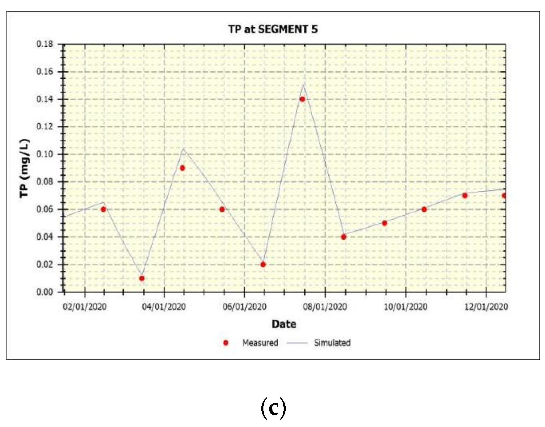
Based on the WASP model parameters calibrated, monitoring data of AN, COD and TP from the year 2020 were used for the validation. The simulation results of each segment of the Lushui River in wet, dry and normal water seasons are shown in Table 12, and Figure 3 shows the comparison of the simulation results and measured data of COD, AN and TP in Segment 5.
The comparison of the simulation results and measured data of COD, AN and TP in Segment 5 (2020) are shown in Figure 3.
3.4. Water Environment Capacity
The calibrated WASP model was used to calculate the pollutant effluent concentration of each river section as the upstream inflow water concentration of the following river section. The results for the water environmental capacity of ammonia nitrogen, COD, and total phosphorus in wet, dry, and normal water seasons are shown in Table 13.
4. Discussion
4.1. Generalization and Polltion Load
The results from the annual average total pollution load of COD, AN and TP in Lushui River from 2019-2020 showed that loads in Segment 3 and Segment 6 were smaller than other segments (shown in Table 2 and Table 3). Additionally, it was shown that the load value in Segment 4 was higher than other segments because there was an intersection of Lushui River with the primary river (Yangtze River). The loads reduced in the middle segments of the river where the area is characterized by urban land use and small-scale urban agriculture. The greatest improvement was observed at the most polluted segment of the Lushui River, which is situated precisely in Segment 1. It could therefore be contributing to the high change in the pollutant load.
4.2. Parameter Sensitivity Analysis
The sensitivity analysis conducted on WASP (Table 10) was performed by varying the parameters by (–50%, +50%). The sensitivity analysis result revealed that six parameters (K12, Θ12, K83, Θ83, Kd and Θd)were identified as medium to highly influential. The sensitivity index of all these parameters were above 0.05, indicating that they are the key parameters affecting the simulated output concentration, according to the model parameter sensitivity analysis (Table 6 and Table 10). The high sensitivity of these parameters was also reported by Guo et al. [25].
4.3. Simulation Results and Model Verification
We used WASP to simulate and analyze the water quality of the Lushui River in 2020 during the normal, dry, and wet water seasons (Table 12, Figure 3). The concentration change trend of each water quality index in the three water seasons was the same. The concentration of COD was normal water seasons > dry water seasons > wet water seasons, and the concentration of AN was normal water seasons > wet water seasons > dry water seasons. The concentration of TP did not change much with the three water seasons. At the same time, from the perspective of seasonal characteristics, the concentrations of COD, TP and AN in different water periods differed mainly due to the large precipitation during the high water period, which led to the release of endogenous pollution in the river sediments. In this regard, there have been related research reports abroad. For example, Hu et al. used the WASP model for the simulation of sediment release items and found that endogenous phosphorus pollution had become a factor that could not be ignored in water quality changes [22]; whereas ammonia nitrogen and COD had different water periods. The main reason was the change of river flow. Rainfall is abundant during the high water period and the river flow is relatively large, which had a certain dilution effect on the pollutants in the river.
4.4. Model Verification and Model Accuracy Evaluation
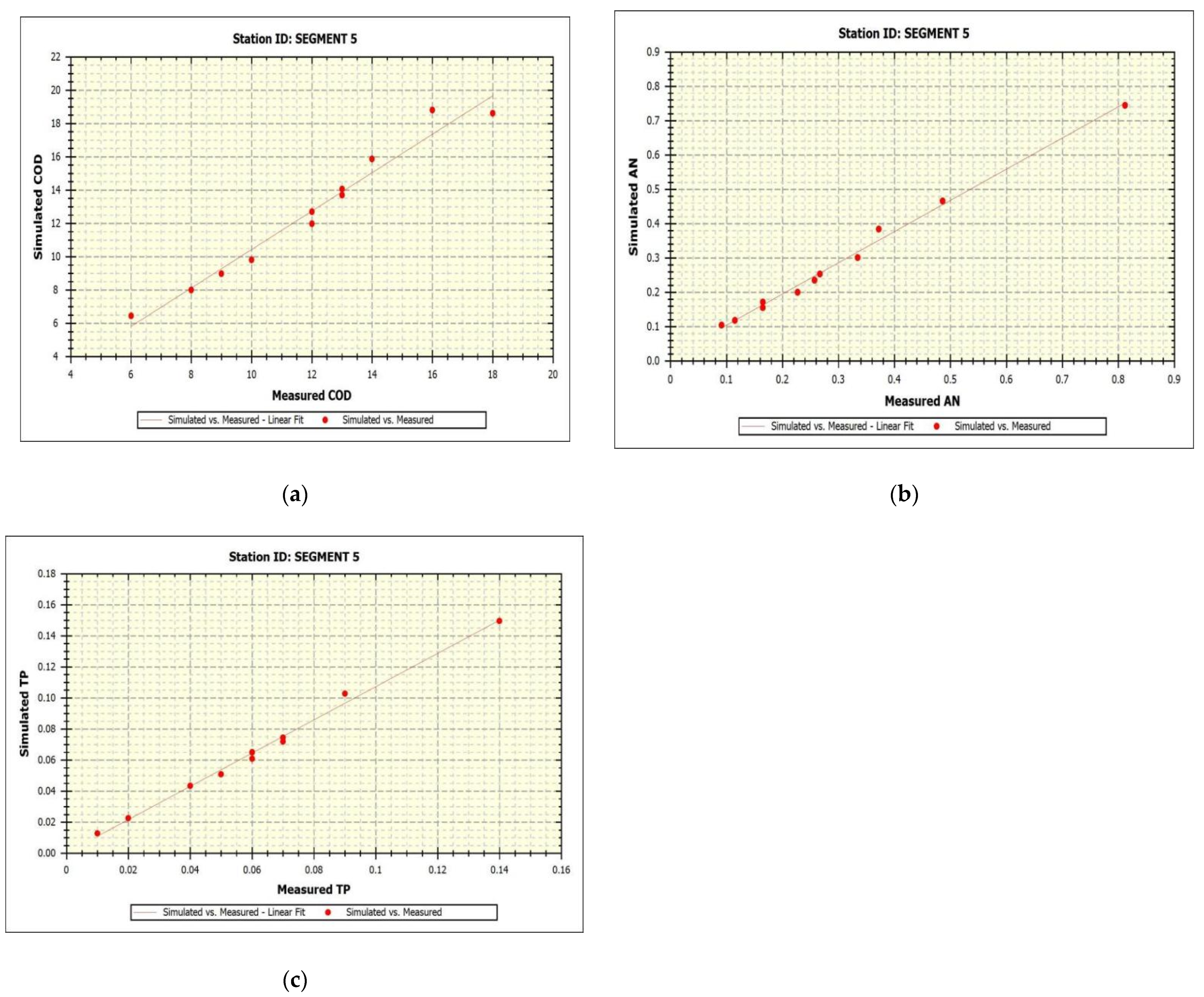
Segment 5 was selected as the model verification segment. The simulation results of this segment from January to December 2020 were used, and then compared with the measured value. The relative error (f) results are shown in Table 14, and the WRDB on WASP was used to perform linear regression analysis on the simulated and measured values to discuss the degree of agreement. For details, see Figure 4.
According to the error analysis results (Table 14), the average relative error between the simulated value of ammonia nitrogen and the measured value was 7.418%. There were 11 groups (12 groups in total) with a relative error of less than 15%, accounting for 91.66%. The average relative error of the simulated COD value and the measured value was 6.086%, of which 11 groups (12 groups in total) had a relative error of less than 15%, accounting for 91.66%. The average relative error of the simulated total phosphorus value and the measured value was 8.637%. The relative error was that there were 10 groups (12 groups in total) less than 15%, accounting for 83.33%. Table 14 shows that the WASP model can be used as an effective tool for water quality prediction and management in the area. The linear regression equation and the accuracy evaluation statistics of the simulation results of COD, AN and TP in Segment 5 (2020) are shown in Figure 4 and Table 15.
The coefficient of determination (R2) sets the fit between monitored and simulated data, and its range value is from 0 to 1. If R2 was close to 1, the model simulation fit satisfactorily with measured data. It can be seen from Figure 4 and Table 15 that the determination coefficients R2 were all above 0.85 and the Index of Agreement (r) were all above 0.90, indicating that the simulated values were in good agreement with the monitored values and had a reasonable correlation. Similar findings relating to the overall effectiveness of water quality simulation studies in other domestic basins were reported by Guo et al. [25].
4.5. Water Environmental Capacity
The water environment capacity of AN, TP and COD in most river sections during dry seasons was smaller than that in normal and wet seasons. This was mainly due to the abundant precipitation in wet seasons, the larger river flow, and the larger water dilution environment capacity. In addition, from Table 6, it can be seen that the environmental capacity of each segment based on the water environment function was quite different, which was mainly affected by the water environment function zoning. When the water environment function was landscape recreation water area and industrial water area, the water environment capacity was relatively large; when the water environment function was a drinking water source protection area, the water environment capacity was relatively small. On the whole, the environmental capacity of the control unit based on human health benchmarks was much smaller than that of the control unit based on the water function zone standard. It can be seen that rivers frequently alternate functional zoning, protection operations are difficult, and management is inconvenient. Although the water quality can meet the standard, it does not guarantee human health very well.
The reductions in pollution load required to meet the water quality objectives were calculated by comparing the pollution load emissions from the water environmental capacity of the Lushui River [11]. Negative values indicated that the environmental capacity remained surplus to the pollution load and has no need to be reduced. Positive values of reduction indicated that the pollution load exceeded the environmental capacity and needs to be reduced. From the perspective of seasonal characteristics, according to the results from the environmental capacity and the pollution load emissions, the reduction in COD, TP and AN in different water periods was around 10 to 15%, meaning that there is a need for reduction. Therefore, in order to achieve the water quality target in the Lushui River, further research is needed to strengthen pollution source prevention and supervision.
5. Conclusions
In order to respond to the national protection policy for the Lushui River, a one-dimensional mathematical model of the water environment was established to study the water environment capacity of ammonia nitrogen, COD and total phosphorus of the Lushui River. In this research, the WASP model was calibrated and validated using data for the years 2019–2020. The calibration results showed that, for ammonia nitrogen, only Θ12 had high sensitivity, K12 had medium sensitivity, and the sensitivity of the remaining parameters were small to negligible. Additionally, for the parameter sensitivity of COD, Θd had high sensitivity, Kd had medium sensitivity, and the sensitivity of the remaining parameters were small to negligible. Furthermore, for total phosphorus, Θ12 had very high sensitivity, Θ83 had high sensitivity, K83 had medium sensitivity, and the sensitivity of the other parameters were small to negligible.
After the calibration process, the simulation results in the year 2020 were verified by all of the determination coefficients R2 being above 0.85, and all of the correlation coefficients r being above 0.90. Therefore, this information indicates that the WASP model is applicable and reliable.
The water environmental capacities were obtained by calibrated parameters on the WASP model using the trial and error method. During the normal, wet and dry water seasons, the COD values were 14,072.94 tons/yr, 17,147.7 tons/yr and 10,998.18 tons/yr, respectively. However, during the normal, wet and dry water seasons, the results for ammonia nitrogen were 469.098 tons/yr, 571.59 tons/yr and 366.606 tons/yr, respectively. Moreover, total phosphorus was 93.8196 tons/yr, 114.318 tons/yr and 73.3212 tons/yr, respectively. Therefore, the results from the WASP model are applicable and reliable and can be used as an effective tool for water quality prediction and assessment in the Lushui River. It can also provide decision-making references for water environmental protection and management in the Lushui River.
Author Contributions
Conceptualization, N.O. and H.T.; methodology, N.O.; software, N.O.; validation, N.O., H.T. and X.L.; formal analysis, N.O.; investigation, N.O., H.T. and X.L.; writing—original draft preparation, N.O.; writing—review and editing, N.O., H.T. and X.L.; visualization, N.O.; supervision, F.G. and X.L.; project administration, X.L. All authors have read and agreed to the published version of the manuscript.
Funding
This research received no external funding.
Institutional Review Board Statement
Not applicable.
Informed Consent Statement
Not applicable.
Data Availability Statement
Not applicable.
Acknowledgments
This research was supported by the Ecological Environmental Protection Technology and Plan of Yangtze River in Zhuzhou City, Project Number: 2019-LHYJ-01-0212-31, and also was also supported by Investigation and Risk Assessment of Ecological Environment Problems in Key Cities of Yangtze River in Economic Zone, Project Number: 2018CJA030301-036. We would like to extend special thanks to the editor and the anonymous reviewers for their valuable comments in greatly improving the quality of this paper.
Conflicts of Interest
The authors declare no conflict of interest.
References
- Fonseca, B.M.; De Mendonça-Galvão, L.; Padovesi-Fonseca, C. Nutrient baselines of Cerrado low-order streams: Comparing natural and impacted sites in Central Brazil. Environ. Monit. Assess. 2014, 186, 19. [Google Scholar] [CrossRef]
- Brooks, B.W.; Riley, T.M.; Taylor, R.D. Water quality of effluent-dominated ecosystems: Ecotoxicological, hydrological, and management considerations. Hydrobiologia 2006, 556, 365–379. [Google Scholar] [CrossRef]
- Zhang, M.L.; Shen, Y.M.; Guo, Y. Development and application of an eutrophication water quality model for river networks. Hydrodynamics 2008, 20, 719–726. [Google Scholar] [CrossRef]
- Ellina, G.; Papaschinopoulos, G.; Papadopoulos, B.K. Research of fuzzy implications via fuzzy linear regression in data analysis for a fuzzy model. J. Comput. Methods Sci. Eng. 2020, 20, 879–888. [Google Scholar] [CrossRef]
- Hu, X. Research on Water Quality Management of Xiangtan Section of Yangtze River Based on WASP Model; Xiangtan University: Xiangtan, China, 2013. (In Chinese) [Google Scholar]
- Lin, J.; Huang, J.-L.; Du, P.-F.; Tu, Z.-S.; Li, Q.-S. Local sensitivity and stability analysis of parameters in urban rainfall runoff hydrological simulation. Environ. Sci. 2010, 31, 2023–2028. [Google Scholar]
- Moriasi, D.N.; Gitau, M.W.; Pai, N.; Daggupati, P. Hydrologic and Water Quality Models: Performance Measures and Evaluation Criteria. Trans. ASABE 2015, 58, 1763–1785. [Google Scholar]
- American Public Health Association; American Water Works Association. Standard Methods for the Examination of Water and Wastewater, 14th ed.; Method 508; American Public Health Association (APHA): Washington, DC, USA, 1975; p. 550. [Google Scholar]
- Ma, L.; Adornato, R.H.; Byrne, D. Yuan Determination of nanomolar levels of nutrients in seawater. Trends Anal. Chem. 2014, 60, 1–15. [Google Scholar] [CrossRef]
- Elser, J.J. Phosphorus: A limiting nutrient for humanity? Curr. Opin. Biotechnol. 2012, 23, 833–838. [Google Scholar] [CrossRef]
- H Šraj, L.O.; Almeida, M.I.G.S.; Swearer, S.E.; Kolev, S.D.; McKelvie, I.D. Analytical challenges and advantages of using flow-based methodologies for ammonia determination in estuarine and marine waters. Trends Anal. Chem. 2014, 59, 83–92. [Google Scholar] [CrossRef]
- Standard. Surface Water Environmental Quality Standard (GB3838-2002); Ministry of Environmental Protection of the People’s Republic of China: Beijing, China, 2002. (In Chinese)
- Seo, I.W.; Baek, K.O. Estimation of the Longitudinal Dispersion Coefficient Using the Velocity Profile in Natural Streams. J. Hydraul. Eng. 2004, 130, 227–236. [Google Scholar] [CrossRef]
- Wijaya, D.S.; Juwan, I. Identification and Calculation of Pollutant Load in Ciwaringin Watershed, Indonesia: Domestic Sector and Faculty of Civil Engineering and Planning; Insttitut Teknologi Nasional Bandung: West Java, Indonesia, 2017. [Google Scholar]
- Xiao, K.X.; Wei, Y.; Ke-feng, L. Estimation and discussion of non-point source pollution loads with new Flux method in Danjiangkou Reservoir area, China. 2016. Available online: https://www.researchgate.net/publication/317291492_Estimation_and_discussion_of_non-point_source_pollution_loads_with_new_Flux_method_in_Danjiangkou_Reservoir_area_China (accessed on 5 October 2021).
- Gu, L.; Hua, Z. Research progress in determining the longitudinal dispersion coefficient of natural rivers. Adv. Sci. Technol. Water Resour. Hydropower 2007, 27, 85–89. [Google Scholar]
- Fischer, H.B. Discussion of Simple Method for Predicting Dispersion in Streams. Keefer. J. Environ. Eng. Div. 1975, 101, 453–455. [Google Scholar] [CrossRef]
- Mcquivey, R.S.; Keefer, T.N. Simple method for predicting dispersion in streams. J. Environ. Eng. Div. 1974, 100, 997–1011. [Google Scholar] [CrossRef]
- Tufford, D.L.; McKellar, H.N. Spatial and temporal hydrodynamic and water quality Modelling analysis of a large reservoir on the South Carolina (USA) coastal plain. Ecol. Model. 1999, 114, 137–173. [Google Scholar] [CrossRef]
- Bae, S.; Seo, D. Analysis and modelling of algal blooms in the Nakdong River. Korea Ecol. Model 2018, 372, 53–63. [Google Scholar] [CrossRef]
- Lenhart, T.; Eckhardt, K.; Fohrer, N. Comparison of two different approaches of sensitivity analysis. Phys. Chem. Earth 2002, 27, 645–654. [Google Scholar] [CrossRef]
- Francos, A.; Elorza, F.J.; Bouraoui, F. Sensitivity analysis of distributed environmental simulation models: Understanding the model behaviour in hydrological studies at the catchment scale. Reliab. Eng. Syst. Saf. 2003, 79, 205–218. [Google Scholar] [CrossRef]
- Peng, S. Research on Uncertainty Water Quality Model Based on WASP Model; Tianjin University: Tianjin, China, 2010. (In Chinese) [Google Scholar]
- Allen, J.I.; Holt, J.T.; Blackford, J.; Proctor, R. Error quantification of a high-resolution coupled hydrodynamic-ecosystem coastal-ocean model: Part 2. Chlorophyll-a, nutrients and SPM. Mar. Syst. 2007, 68, 381–404. [Google Scholar]
- Guo, X.; Yan, S. Sensitivity analysis of rigid pile composite foundation model parameters based on orthogonal design method. J. Self -Sci. Xiangtan Univ. 2015, 37, 15–20. [Google Scholar]
- Cerny, V. Thermodynamical approach to the traveling salesman problem: An efficient simulation algorithm. Optimiz. Theory App. 1985, 45, 41–51. [Google Scholar] [CrossRef]
- Putnam, H. Trial and error predicates and the solution to a problem of Mostowski. Symb. Logic. 1965, 30, 49–57. [Google Scholar] [CrossRef]
- Refsgaard, J.C.; Knudsen, J. Operational validation and intercomparison of different types of hydrological models. Water Resour. Res. 1996, 32, 2189–2202. [Google Scholar] [CrossRef]
- Liu, X. The Heavy Metal Water Quality Target Management Research on Yangtze River Based on Human Health Risk; Central South University: Changsha, China, 2017. (In Chinese) [Google Scholar]
- Sin, G.; de Pauw, D.J.W.; Weijers, S.; Vanrolleghem, P.A. An efficient approach to automate the manual trial and error calibration of activated sludge models. Biotechnol. Bioeng. 2008, 100, 516–528. [Google Scholar] [CrossRef]
- Nash, J.E.; Sutcliffe, J.V. River flow forecasting through conceptual models part I—A discussion of principles. Hydrology 1970, 10, 282–290. [Google Scholar] [CrossRef]
Figure 1.
Overview of the research area.
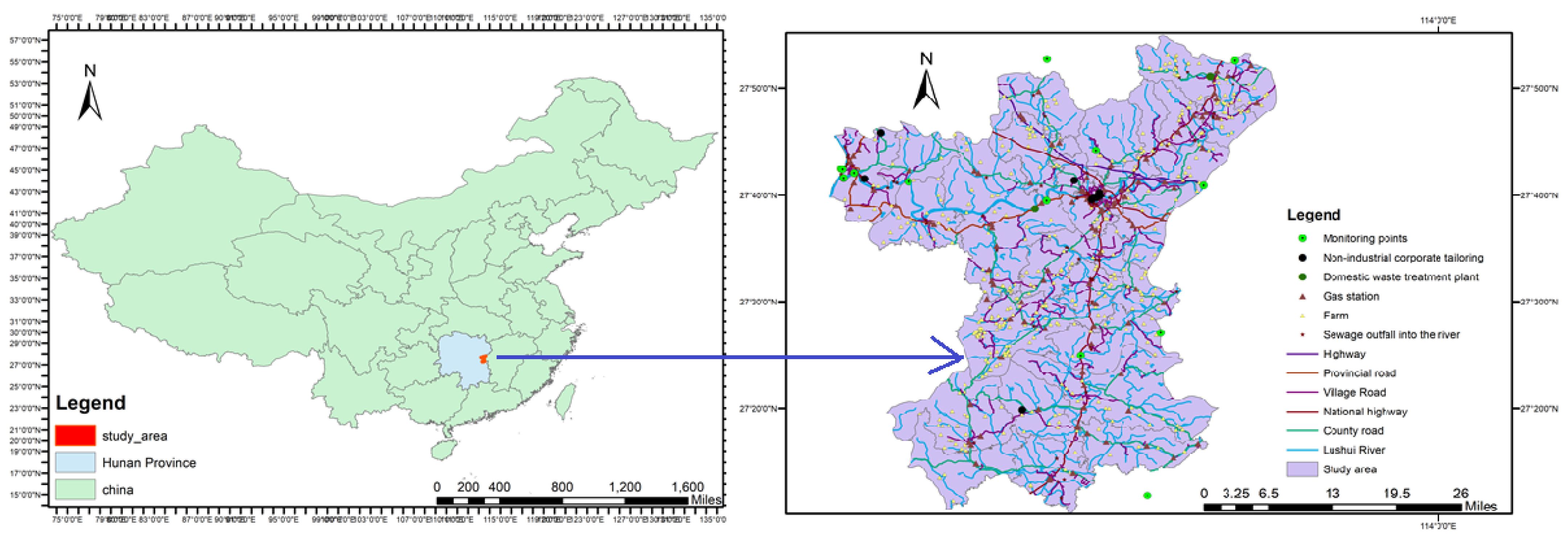
Figure 2.
Division of control units and segmentation in the study area.
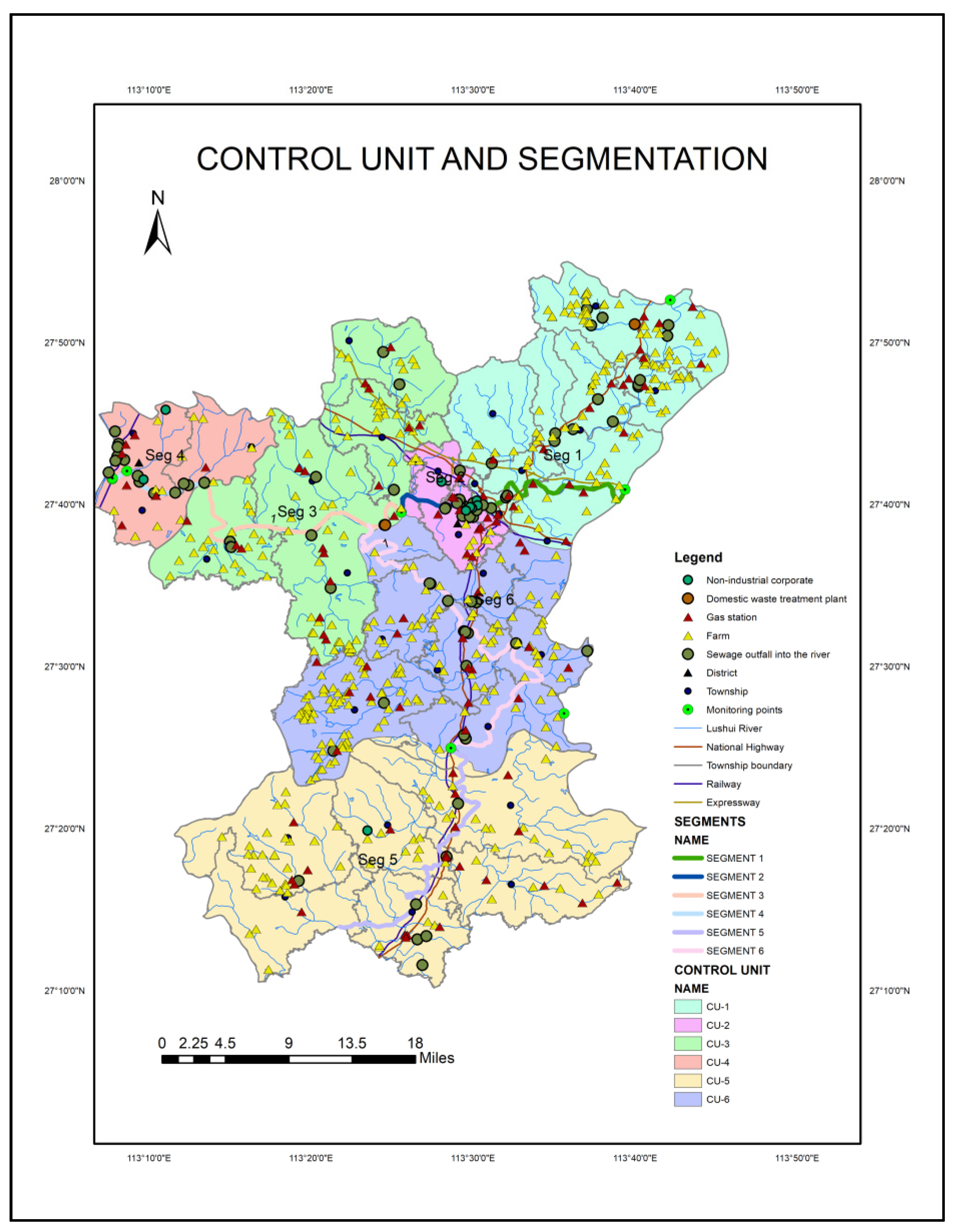
Figure 3.
(a), (b) and (c) Comparison of the simulation results and measured data of COD, AN and TP in Segment 5 (2020).
Figure 3.
(a), (b) and (c) Comparison of the simulation results and measured data of COD, AN and TP in Segment 5 (2020).
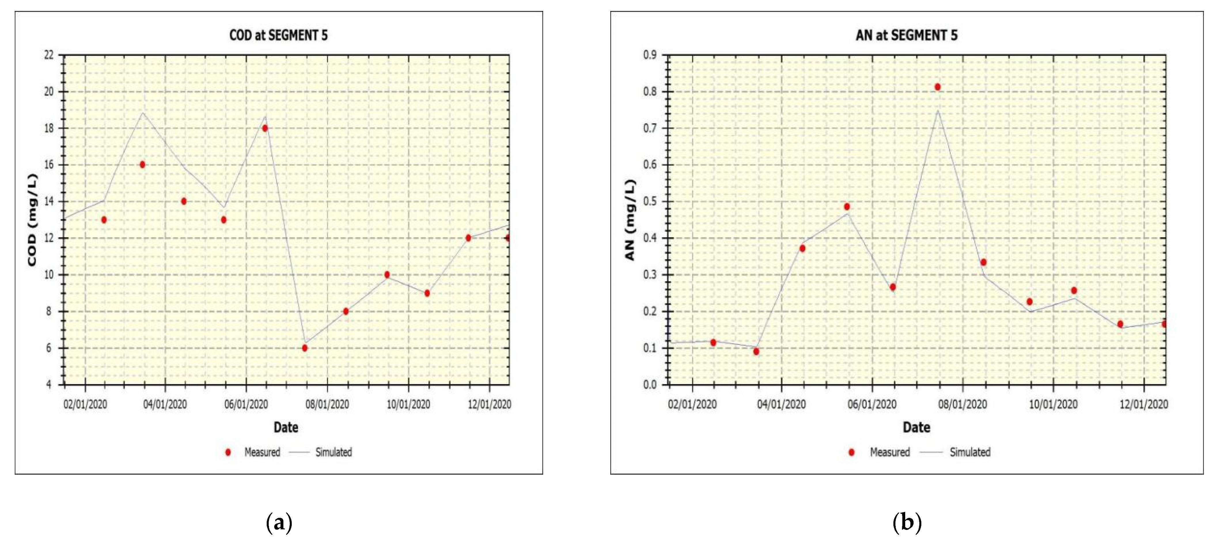

Figure 4.
(a–c) Linear regression equation of COD, AN and TP in Segment 5 (2020).


Table 1.
Segment information of Lushui River.
| Segment | Volume | Velocity Mult | Depth Mult | Length | Width | Slope | Bottom Rough |
| 1 | 9.43 × 10⁵ | 1.05 | 1 | 2.21 × 10⁴ | 42.74 | 9.97 × 10⁴ | 0.03 |
| 2 | 9.94 × 10⁵ | 1.26 | 1.5 | 1.20 × 10⁴ | 55.42 | 8.36 × 10⁴ | 0.03 |
| 3 | 4.72 × 10⁶ | 0.89 | 2 | 3.18 × 14 | 74.17 | 2.82 × 10⁴ | 0.03 |
| 4 | 3.18 × 10⁶ | 1.55 | 3 | 1.20 × 10⁴ | 88.47 | 5.01 × 10⁴ | 0.03 |
| 5 | 1.51 × 10⁶ | 0.98 | 1 | 5.46 × 10⁴ | 27.61 | 8.60 × 10⁴ | 0.03 |
| 6 | 1.82 × 10⁶ | 1.04 | 1.3 | 3.79 × 10⁴ | 36.99 | 6.85 × 10⁴ | 0.03 |
Mult = multiplier; rough = roughness; the unit of volume is m3; the unit of length, width and depth are m, and the unit of velocity is m/s.
Table 2.
Annual average total pollution load of COD, AN and TP in the Lushui River in 2019 (kg/d).
| Segment | COD | AN | TP |
|---|---|---|---|
| Segment 1 | 26769.6 | 1031.616 | 277.416 |
| Segment 2 | 29318.4 | 1226.751 | 305.424 |
| Segment 3 | 22910.4 | 359.452 | 187.704 |
| Segment 4 | 210024 | 6440.76 | 2496.268 |
| Segment 5 | 28687.68 | 681.883 | 140.112 |
| Segment 6 | 26618.4 | 506.800 | 124.56 |
Table 3.
Annual average total pollution load of COD, AN and TP in the Lushui River in 2020 (kg/d).
| Segments | COD | AN | TP |
|---|---|---|---|
| Segment 1 | 46656 | 747.468 | 226.8 |
| Segment 2 | 42026.4 | 706.176 | 153.216 |
| Segment 3 | 25934.4 | 301.176 | 261.432 |
| Segment 4 | 286387.2 | 4972.032 | 2865.384 |
| Segment 5 | 28296 | 427.104 | 110.664 |
| Segment 6 | 24429.6 | 361.44 | 78.192 |
Table 4.
Corresponding longitudinal dispersion coefficients for each segment (m2/s).
| Segments | EX | Segments | EX |
|---|---|---|---|
| Segment 1 | 43.047 | Segment 4 | 405.725 |
| Segment 2 | 48.939 | Segment 5 | 62.246 |
| Segment 3 | 79.564 | Segment 6 | 53.134 |
Table 5.
Determination of initial boundary concentration.
| Boundary | COD (mg/L) | AN (mg/L) | TP (mg/L) |
|---|---|---|---|
| Segment 1 | 13.5 | 0.284 | 0.09 |
| Segment 4 | 10 | 0.12 | 0.1 |
| Segment 5 | 13 | 0.31 | 0.06 |
Table 6.
Sensitivity classes [7].
Table 6.
Sensitivity classes [7].
| Sensitivity Index | Grading Standard | Level |
|---|---|---|
| 0.00 ≤ SS ≤ 0.05 | Small to negligible | 1 |
| 0.05 ≤ SS ≤ 0.20 | Medium | 2 |
| 0.20 ≤ Ss ≤ 1.00 | High | 3 |
| Ss ≥ 1.00 | Very high | 4 |
Table 7.
Theory optimal parameter combination of COD, AN and TP.
| K12 | Θ12 | K83 | Θ83 | Kd | Θd |
|---|---|---|---|---|---|
| 0.0972 | 0.832 | 0.144 | 0.856 | 0.2772 | 0.8376 |
Table 8.
General performance ratings of the recommended statistics.
| Measure | Coefficient of Determination | Performance Rating |
|---|---|---|
| 0.00 ≤ R2 ≤0.40 | Unsatisfactory | |
| R2 | 0.40 ≤ R2 ≤ 0.60 | Satisfactory |
| 0.60 ≤ R2 ≤ 0.75 | Good | |
| 0.75 ≤ R2 ≤ 1 | Very Good |
Table 9.
Standards values of surface water environmental quality (GB3838-2002) (unit: mg/L).
| Indicators | I | II | III | IV |
| COD | 15 | 15 | 20 | 30 |
| AN | 0.15 | 0.5 | 1.0 | 1.5 |
| TP | 0.02 | 0.1 | 0.2 | 0.3 |
Table 10.
Parameter sensitivity calculation.
| Symbol | COD | AN | TP | |||||||||
|---|---|---|---|---|---|---|---|---|---|---|---|---|
| (−50%) | (+50%) | SS | Class | (−50%) | (+50%) | SS | Class | (−50%) | (+50%) | SS | Class | |
| K12 * | 0 | 0.000 | 0.000 | 1 | 0.025 * | 0.075 * | 0.05 * | 2 * | 0 | 0 | 0 | 1 |
| Θ12 * | 0 | 0.000 | 0.000 | 1 | 0.369 * | 0.387 * | 0.378 * | 3 * | 0 | 2.062 * | 1.031 * | 4 * |
| KNO3 | 0 | 0.000 | 0.000 | 1 | 0.001 | 0.003 | 0.002 | 1 | 0 | 0 | 0 | 1 |
| Tmin | 0 | 0.000 | 0.000 | 1 | 0 | 0 | 0 | 1 | 0 | 0 | 0 | 1 |
| K2D | 0 | 0.000 | 0.000 | 1 | 0 | 0 | 0 | 1 | 0 | 0 | 0 | 1 |
| Θ2D | 0 | 0.000 | 0.000 | 1 | 0 | 0 | 0 | 1 | 0 | 0 | 0 | 1 |
| KNO3 | 0.000 | 0.000 | 0.000 | 1 | 0 | 0 | 0 | 1 | 0 | 0 | 0 | 1 |
| K71 | 0.000 | 0.000 | 0.000 | 1 | 0 | 0 | 0 | 1 | 0 | 0 | 0 | 1 |
| K83 * | 0.000 | 0.000 | 0.000 | 1 | 0 | 0 | 0 | 1 | 0 | 0.111 * | 0.055 * | 2 * |
| Θ71 | 0.000 | 0.000 | 0.000 | 1 | 0 | 0 | 0 | 1 | 0 | 0 | 0 | 1 |
| Θ83 * | 0.000 | 0.000 | 0.000 | 1 | 0 | 0 | 0 | 1 | 0.44 * | 0.413 * | 0.427 * | 3 * |
| Kd * | 0.065 * | 0.196 * | 0.131 * | 2 * | 0 | 0 | 0 | 1 | 0 | 0 | 0 | 1 |
| Θd * | 0.319 * | 0.612 * | 0.465 * | 3 * | 0 | 0 | 0 | 1 | 0 | 0 | 0 | 1 |
| KCOD | 0.003 | 0.009 | 0.006 | 1 | 0 | 0 | 0 | 1 | 0 | 0 | 0 | 1 |
| fD5 | 0.000 | 0.000 | 0.000 | 1 | 0 | 0 | 0 | 1 | 0 | 0 | 0 | 1 |
| R | 0.000 | 0.000 | 0.000 | 1 | 0 | 0 | 0 | 1 | 0 | 0 | 0 | 1 |
The parameters with an asterisk (*) are the key parameters affecting the simulated output concentration.
Table 11.
Model parameter calibration results.
| Parameter Name | Symbol | Value | Unit |
|---|---|---|---|
| Nitrification Rate Constant at 20 °C | K12 | 0.081 | d−1 |
| Nitrification Temperature Coefficient | Θ12 | 1.04 | |
| Half Saturation Constant for Nitrification Oxygen Limit | KNO3 | 0.5 | mgO2/L |
| Minimum Temperature for Nitrification Reaction | Tmin | 3 | °C |
| Denitrification Rate Constant at 20 °C | K2D | 0.045 | d−1 |
| Denitrification Temperature Coefficient | Θ2D | 1.04 | |
| Half Saturation Constant for Denitrification Oxygen Limit | KNO3 | 0.1 | mgO2/L |
| Dissolved Organic Nitrogen Mineralization Rate Constant at 20 °C | K71 | 0.075 | d−1 |
| Dissolved Organic Phosphorus Mineralization Rate Constant at 20 °C | K83 | 0.12 | d−1 |
| Dissolved Organic Nitrogen Mineralization Temperature Coefficient | Θ71 | 1.08 | |
| Dissolved Organic Phosphorus Mineralization Temperature Coefficient | Θ83 | 1.07 | |
| COD Decay Rate Constant at 20 °C | Kd | 0.231 | d−1 |
| COD Decay Rate Temperature Correction Coefficient | Θd | 1.047 | |
| COD Half Saturation Oxygen Limit | KCOD | 0.5 | mgO2/L |
| Fraction of Detritus Dissolution to COD | f D5 | 0.2 | |
| Fraction of COD Carbon Source for Denitrification | R | 0.2 |
Table 12.
Simulation results of concentrations in normal, dry and wet seasons (2020).
| Segments | COD | AN | TP | ||||||
|---|---|---|---|---|---|---|---|---|---|
| Normal | Wet | Dry | Normal | Wet | Dry | Normal | Wet | Dry | |
| Segment 1 | 8.837 | 5.223 | 8.654 | 0.392 | 0.314 | 0.418 | 0.130 | 0.097 | 0.105 |
| Segment 2 | 19.140 | 9.468 | 13.320 | 0.731 | 0.469 | 0.795 | 0.191 | 0.160 | 0.195 |
| Segment 3 | 12.376 | 7.732 | 9.623 | 0.325 | 0.243 | 0.325 | 0.095 | 0.092 | 0.110 |
| Segment 4 | 38.393 | 44.830 | 38.922 | 1.355 | 1.258 | 0.844 | 0.425 | 0.645 | 0.290 |
| Segment 5 | 15.609 | 10.697 | 11.671 | 0.269 | 0.374 | 0.218 | 0.061 | 0.067 | 0.067 |
| Segment 6 | 16.141 | 10.712 | 10.229 | 0.263 | 0.373 | 0.157 | 0.071 | 0.068 | 0.063 |
Table 13.
Water capacity results (tons/year).
| Segments | COD | AN | TP | ||||||
|---|---|---|---|---|---|---|---|---|---|
| Normal | Wet | Dry | Normal | Wet | Dry | Normal | Wet | Dry | |
| Segment 1 | 14,072.94 | 17,147.7 | 10,998.18 | 469.098 | 571.59 | 366.606 | 93.8196 | 114.318 | 73.3212 |
| Segment 2 | 21,286.8 | 19,512.9 | 17,975.52 | 709.56 | 650.43 | 599.184 | 141.912 | 130.086 | 119.8368 |
| Segment 3 | 13,481.64 | 14,427.72 | 11,944.26 | 449.388 | 480.924 | 398.142 | 89.8776 | 96.1848 | 79.6284 |
| Segment 4 | 135,525.96 | 185,195.16 | 85,738.5 | 4517.532 | 6173.17 | 2857.95 | 903.5064 | 1234.634 | 571.59 |
| Segment 5 | 15,846.84 | 12,417.3 | 10,288.62 | 528.228 | 413.91 | 342.954 | 105.6456 | 82.782 | 68.5908 |
| Segment 6 | 12,949.47 | 12,831.21 | 7686.9 | 431.649 | 427.707 | 256.23 | 86.3298 | 85.5414 | 51.246 |
| Total | 14,072.94 | 17,147.7 | 10,998.18 | 469.098 | 571.59 | 366.606 | 93.8196 | 114.318 | 73.3212 |
Table 14.
Error analysis of simulation results 2020.
| Date (MM/DD/YY) | COD | AN | TP | ||||||
|---|---|---|---|---|---|---|---|---|---|
| Simulated | Observed | f | Simulated | Observed | f | Simulated | Observed | f | |
| 1/15/2020 | 13.000 | 12 | 8.33% | 0.115 | 0.107 | 7.04% | 0.055 | 0.05 | 9.79% |
| 2/15/2020 | 14.083 | 13 | 8.33% | 0.118 | 0.115 | 2.98% | 0.065 | 0.06 | 8.25% |
| 3/15/2020 | 18.842 | 16 | 17.76% | 0.105 | 0.091 | 15.09% | 0.012 | 0.01 | 24.86% |
| 4/15/2020 | 15.831 | 14 | 13.08% | 0.387 | 0.372 | 4.02% | 0.104 | 0.09 | 15.23% |
| 5/15/2020 | 13.682 | 13 | 5.25% | 0.466 | 0.486 | 4.12% | 0.065 | 0.06 | 7.54% |
| 6/15/2020 | 18.629 | 18 | 3.50% | 0.252 | 0.267 | 5.46% | 0.022 | 0.02 | 11.65% |
| 7/15/2020 | 6.313 | 6 | 5.21% | 0.749 | 0.812 | 7.82% | 0.151 | 0.14 | 7.73% |
| 8/15/2020 | 8.019 | 8 | 0.24% | 0.296 | 0.334 | 11.40% | 0.042 | 0.04 | 5.63% |
| 9/15/2020 | 9.828 | 10 | 1.72% | 0.199 | 0.227 | 12.38% | 0.051 | 0.05 | 2.11% |
| 10/15/2020 | 8.979 | 9 | 0.24% | 0.235 | 0.257 | 8.50% | 0.061 | 0.06 | 1.67% |
| 11/15/2020 | 12.007 | 11.8 | 1.76% | 0.155 | 0.165 | 6.31% | 0.072 | 0.07 | 2.88% |
| 12/15/2020 | 12.700 | 11.8 | 7.62% | 0.171 | 0.165 | 3.90% | 0.074 | 0.07 | 6.31% |
Table 15.
Accuracy evaluation statistics of the simulation results in Segment 5: January 1, 2020– December 31, 2021.
Table 15.
Accuracy evaluation statistics of the simulation results in Segment 5: January 1, 2020– December 31, 2021.
| COD | AN | TP | ||||
|---|---|---|---|---|---|---|
| Statistics | Measured | Simulated | Measured | Simulated | Measured | Simulated |
| Count | 12 | 12 | 12 | 12 | 12 | 12 |
| Min | 6.000 | 6.313 | 0.091 | 0.104 | 0.010 | 0.012 |
| Max | 18.000 | 18.842 | 0.812 | 0.749 | 0.140 | 0.151 |
| Coef of Det (R2) | 0.97 | 0.99 | 0.99 | |||
| Mean Abs Error | 0.764 | 0.021 | 0.004 | |||
| RMS Error | 1.129 | 0.027 | 0.006 | |||
| Norm RMS Error | 0.088 | 0.078 | 0.079 | |||
| Index of Agreement (r) | 0.98 | 0.99 | 0.99 |
Publisher’s Note: MDPI stays neutral with regard to jurisdictional claims in published maps and institutional affiliations. |
© 2021 by the authors. Licensee MDPI, Basel, Switzerland. This article is an open access article distributed under the terms and conditions of the Creative Commons Attribution (CC BY) license (https://creativecommons.org/licenses/by/4.0/).
Share and Cite
MDPI and ACS Style
Obin, N.; Tao, H.; Ge, F.; Liu, X. Research on Water Quality Simulation and Water Environmental Capacity in Lushui River Based on WASP Model. Water 2021, 13, 2819. https://doi.org/10.3390/w13202819
AMA Style
Obin N, Tao H, Ge F, Liu X. Research on Water Quality Simulation and Water Environmental Capacity in Lushui River Based on WASP Model. Water. 2021; 13(20):2819. https://doi.org/10.3390/w13202819
Chicago/Turabian StyleObin, Nicolas, Hongni Tao, Fei Ge, and Xingwang Liu. 2021. "Research on Water Quality Simulation and Water Environmental Capacity in Lushui River Based on WASP Model" Water 13, no. 20: 2819. https://doi.org/10.3390/w13202819
Note that from the first issue of 2016, this journal uses article numbers instead of page numbers. See further details here.