Analysis of Factors Influencing Effective Utilization Coefficient of Irrigation Water in the Manas River Basin
by
 , , , ,
Lili Yang
1,2 ,
,
Tong Heng
1,2,
Guang Yang
1,2,
Xinchen Gu
1,2,
Jiaxin Wang
1,2 and
Xinlin He
1,2,* 1
College of Water and Architectural Engineering, Shihezi University, Shihezi 832003, China
2
Xinjiang Production and Construction Group Key Laboratory of Modern Water-Saving Irrigation, Shihezi University, Shihezi 832000, China
*
Author to whom correspondence should be addressed.
Water 2021, 13(2), 189; https://doi.org/10.3390/w13020189
Submission received: 26 November 2020
/
Revised: 7 January 2021
/
Accepted: 11 January 2021
/
Published: 14 January 2021
(This article belongs to the Special Issue Sustainable Irrigation Management in Agriculture)
Abstract
:The factors influencing the effective utilization coefficient of irrigation water are not understood well. It is usually considered that this coefficient is lower in areas with large-scale irrigation. With this background, we analyzed the effective utilization coefficient of irrigation water using the analytic hierarchy process using data from 2014 to 2019 in Shihezi City, Xinjiang. The weights of the influencing factors on the effective utilization coefficient of irrigation water in different irrigation areas were analyzed. Predictions of the coefficient’s values for different years were made by understanding the trends based on the grey model. The results show that the scale of the irrigation area is not the only factor determining the effective utilization coefficient of irrigation water. Irrigation technology, organizational integrity, crop types, water price management, local economic level, and channel seepage prevention are the most critical factors affecting the effective use of irrigation water. The grey model prediction results show that the effective utilization coefficient of farmland irrigation water will continuously increase and reach 0.7204 in 2029. This research can serve as a reference for government authorities to make scientific decisions on water-saving projects in irrigation districts in terms of management, operation, and investment.
1. Introduction
Global water demand has drastically increased over the past fifty years, causing problems such as the overexploitation of water resources and imbalance in supply and demand. In arid and semi-arid regions, irrigation water is a critical factor for agricultural development [1]. Water shortages have affected agricultural production [2]. Governments of various countries are trying to ensure the increase of agricultural production through comprehensive and expensive irrigation projects. Water has become an essential strategic resource that affects regional development and stability. Agricultural water accounts for 70% of global freshwater extraction, and the proportion in some parts of the world is as high as 90% [3]. The International Irrigation and Drainage Commission defines irrigation efficiency as the ratio of the actual use of water by a crop to the total water inflow from the head of the canal [4]. As a large agricultural country, China’s utilization coefficient of farmland irrigation water has been maintained at approximately 0.5 for many years, which is far lower than 0.7–0.8 achieved by developed countries.
Research on the factors that affect the effective utilization coefficient of irrigation water has been ongoing. The effective utilization coefficient of irrigation water refers to the ratio of the amount of water that is nonreusable to the water use system to the total amount of water from the head of the main canal [5]. Hussain et al. [6] pointed out that regional resources, agricultural products and technologies, and water supply prices are the most important factors that affect the effective utilization coefficient of irrigation water through research on large-scale irrigation areas. Rodríguez-Díaz et al. [7] applied benchmark testing and multivariate data analysis techniques, such as cluster analysis, to nine irrigation areas in Andalusia, Spain and found that the unit water use cost of farmers has a significant relationship with the effective utilization coefficient of irrigation water. Xiong Jia [8] studied the relationship between irrigation water utilization rate and natural and human-made factors and suggested that the effects of these factors on the effective utilization coefficient of irrigation water are interrelated. Based on analyzing the traditional measurement method used for the irrigation water utilization coefficient, Xu et al. [9] suggested that the scales of irrigation areas, channel levels, antiseepage measures, and irrigation technology levels are the main factors that affect the effective utilization coefficient. Liu et al. [10] found that socioeconomic development level (GDP) and effective irrigation area have significant impacts on the effective utilization coefficient of irrigation water. Qin et al. [11] evaluated the agricultural water-saving potential of China’s Beijing–Tianjin–Hebei region by combining multiple factors and the effective use of irrigation water. Agricultural water saving can also be achieved through improvements in irrigation technology and management [4,12]. There are many reports on the factors affecting the efficiency of irrigation water use; however, research on the degree of influence of each factor on the effective utilization coefficient of irrigation water is lacking.
China has the largest drip irrigation area under mulch on farmland in the world [13]. The Xinjiang Province is the birthplace of China’s drip irrigation technology under mulch, and it has developed irrigated oasis agriculture techniques over many years. Irrigation technology and management experience are relatively advanced, representative, and typical in Xinjiang. At the same time, Xinjiang is located in an inland arid area, and water resources are relatively scarce. Irrigation accounts for 89.4% of the total water consumption of the province [14]. The contradiction between water supply and demand in Xinjiang has become increasingly prominent, and the agricultural water-saving potential is huge. Related research has also been carried out in this region. For instance, Geng and Song [15] used the Tobit model to analyze the influencing factors of irrigation water efficiency in the cotton fields of Xinjiang. Wei [16] carried out calculations on agricultural water use efficiency in various prefectures in Xinjiang and explored the influencing factors of agricultural water use efficiency. However, the effective utilization coefficient of irrigation water in the large-scale Shihezi irrigation district in Xinjiang was higher than that of other medium-sized irrigation districts, which is not consistent with many previous research results [17,18,19,20,21,22]. Therefore, to analyze and identify the factors that significantly affect the utilization coefficient of irrigation water, this study investigated all irrigation areas in the Shihezi district of Xinjiang. We used the analytic hierarchy process to calculate the weight of each factor, and the effective utilization coefficient of irrigation water from 2014 to 2019 to predict the future trend of irrigation water efficiency using the grey model. The outcomes of this research are of practical significance and can serve as a reference for government authorities to make scientific decisions that promote the development of water-saving irrigation.
2. Materials and Methods
2.1. Study Area
The study area (Figure 1) is located at the southern edge of the Junggar Basin in the middle section of the northern slope of the Tianshan Mountains in Shihezi City, Xinjiang, China. It belongs to the Manasi River Basin and is the central area of the economic belt on the northern slope of Tianshan Mountains in Xinjiang. It has an arid continental climate with scarce rainfall. The average annual rainfall during 1965–2018 was 200.5 mm. The rainfall mainly occurs during spring and summer, accounting for 67% of the annual precipitation. Evaporation is extensive, with an annual average of 1500 mm, suggesting a typical desert oasis and irrigated agricultural area. The Manas River is the primary source of water and it is mainly supplied by alpine snowmelt and precipitation. The primary sources of irrigation are river, spring, and well water.
The total irrigated area in the study area is 3094.4 km2 and the cultivated land area is 2740 km2, 93% of which uses drip irrigation under film mulch. Large-scale irrigation areas (irrigated area > 200 km2) include the Mosuowan, Shihezi, Xiayedi, and Anjihai. Medium-sized irrigation areas (33.3 km2 > irrigation area > 200 km2) include Honggou, Ningjiahe, and Da’nangou. Shiyanchang is an irrigation area supplied by wells. The total length of channels in the region is 3349.15 km (of which 2815.46 km is impervious) with a flow rate of more than 0.2 m3/s.
2.2. Data Sources
Statistical data collected by the district authorities in all large and medium-sized irrigation districts and well irrigation districts of Shihezi, Xinjiang from 2014 to 2019 were used for this study. The “calculation method for canal head and tail water” was used to investigate the effective utilization coefficient of irrigation water. Crops covering a planting area of more than 10% of the total irrigation area were selected as typical crops. Three typical fields were selected in each of the upper, middle, and lower reaches of the large-scale irrigation area (a total of 9 typical fields). Three typical fields were selected in the upstream and downstream of the medium-sized irrigation area (a total of 6 typical fields). Four typical fields were selected in the well irrigation area. As the only common crop in each irrigation area is cotton, the planned wet layer was kept at 0.6 m, and samples were drawn at 10-cm depth intervals with a total of 6 layers. Stainless steel cores were used to drill and collect approximately 25 g of soil samples within 48 h before and after each irrigation period. The collected soil samples were stored in an aluminum box (60 mm in diameter, 30 mm in height, and M1 in mass). After the boxes were wrapped with tape, the surface was wiped clean and the aluminum box was sent to the laboratory. There, the box was weighed using a balance with an accuracy of ±0.01 g, and the weight was noted as M2. The soil sample was heated in an oven at 105 °C for 12 h to a constant weight, and this was recorded as M3. The soil moisture content was calculated as follows:
Based on the change in the planned wet layer’s soil moisture content before and after typical field irrigation, the net irrigation water consumption per unit area was calculated using the formula:
where is the net irrigation water consumption per unit area in the field (m3/ha), H is the designated moist layer of soil (m), γ is the bulk density (t/m3), θg1 is the soil water content before irrigation (%), and θg2 is the soil water content after irrigation (%).
The sum of all values was calculated to determine the annual net irrigation water consumption per unit area in a typical field The net irrigation water consumption per unit area of a typical field was calculated as follows:
where is the irrigation area of the typical field (ha) and m is the number of typical fields.
The net irrigation water use (Q7 in Figure 2) was calculated as follows:
where is the number of typical irrigation areas.
The gross irrigation water use (Q1 in Figure 2) was monitored by the local water conservancy department based on the actual water taken from the water source by the irrigation area. The coefficient of water irrigation was calculated as follows:
Other relevant data for this research were procured from the Eighth Division Shihezi City Water Conservancy Statistical Yearbook. The indicator system composition principle was put forward based on data review, expert consultation, field investigation, comprehensive analysis, and consideration of natural and unnatural conditions. This principle led to a selection that accurately reflected the impact of irrigation water use in various types of irrigation areas and was highly targeted. Thirty representative indicators were used to construct an index system for the prediction of the effective utilization coefficient of agricultural irrigation water (Figure 3).
2.3. Analytic Hierarchy Process
The analytic hierarchy process is a systematic analysis method that combines quantitative and qualitative approaches. It involves a multiobjective group decision-making process, which decomposes decision-making goals to different levels to form a bottom-up cascade structure [23]. The indicators are sorted and quantified to form a judgment matrix, and the judgment matrix is checked for consistency, and then the weight is calculated to analyze the correlation and restriction of the hierarchy in the indicator system.
In order to quantify the analysis of A = , i, j = 1, 2, …, n in the matrix, the 1–9 scale method was adopted. The specific values were based on data, systematic analysis, and expert consultation.
Maximum eigenvalue of the matrix and consistency inspection index (CI) were calculated as follows:
where n is the matrix dimension.
The average random consistency index (RI) was selected according to the matrix’s dimension, and its value is shown in Table 1.
When CR < 0.1, it is considered that the consistency check passes. Otherwise the value must be reassigned until the check passes.
The index weight of single-level elements was calculated by
where,
Normalization processing followed:
2.4. Grey Model
Suppose that the equal interval time series has n observations , which are accumulated to form times,
The sequence after the randomness has been weakened by m times can be obtained by: . If is the mean value of the sequence of , , so .
The differential equation of the whitening grey prediction model GM (1,1) was established according to existing data:
where a is the evolution parameter and b is the grey action quantity. According to the principle of least squares, the parameters a and b, and the prediction model are obtained through Laplace transform and inverse Laplace transform:
3. Results
3.1. Weight Analysis of Influencing Factors of Effective Utilization Coefficient of Irrigation Water
A judgment matrix for indicator A was constructed as follows:
| A | B1 | B2 | CI | |
| B1 | 1 | 1/2 | 0.3333 | 0 |
| B2 | 2 | 1 | 0.6667 |
The consistency of the matrix was checked, the maximum eigenvalue = 2 was calculated, and the consistency index was given a value CI = 0, such that the matrix could be judged to be a consistent matrix.
A judgment matrix for indicator B1 was constructed as follows:
| B1 | C1 | C2 | C3 | C4 | C5 | CI | |
| C1 | 1 | 1/2 | 1/3 | 1/4 | 1/6 | 0.0556 | 0.0732 |
| C2 | 2 | 1 | 3 | 1/2 | 1/5 | 0.1411 | |
| C3 | 3 | 1/3 | 1 | 1/3 | 1/4 | 0.0954 | |
| C4 | 4 | 2 | 3 | 1 | 1/3 | 0.2219 | |
| C5 | 6 | 5 | 4 | 3 | 1 | 0.4860 |
The consistency of the matrix was checked, the maximum eigenvalue = 5.2928 was calculated, and the consistency index value was CI = 0.0732, such that the matrix could be judged to be consistent.
A judgment matrix for indicator B2 was constructed as follows:
| B2 | C6 | C7 | CI | |
| C6 | 1 | 1/4 | 0.2000 | 0 |
| C7 | 4 | 1 | 0.8000 |
The consistency of the matrix was checked, the maximum eigenvalue = 2 was calculated, and the consistency index value was CI = 0.0732, such that the matrix could be judged to be consistent.
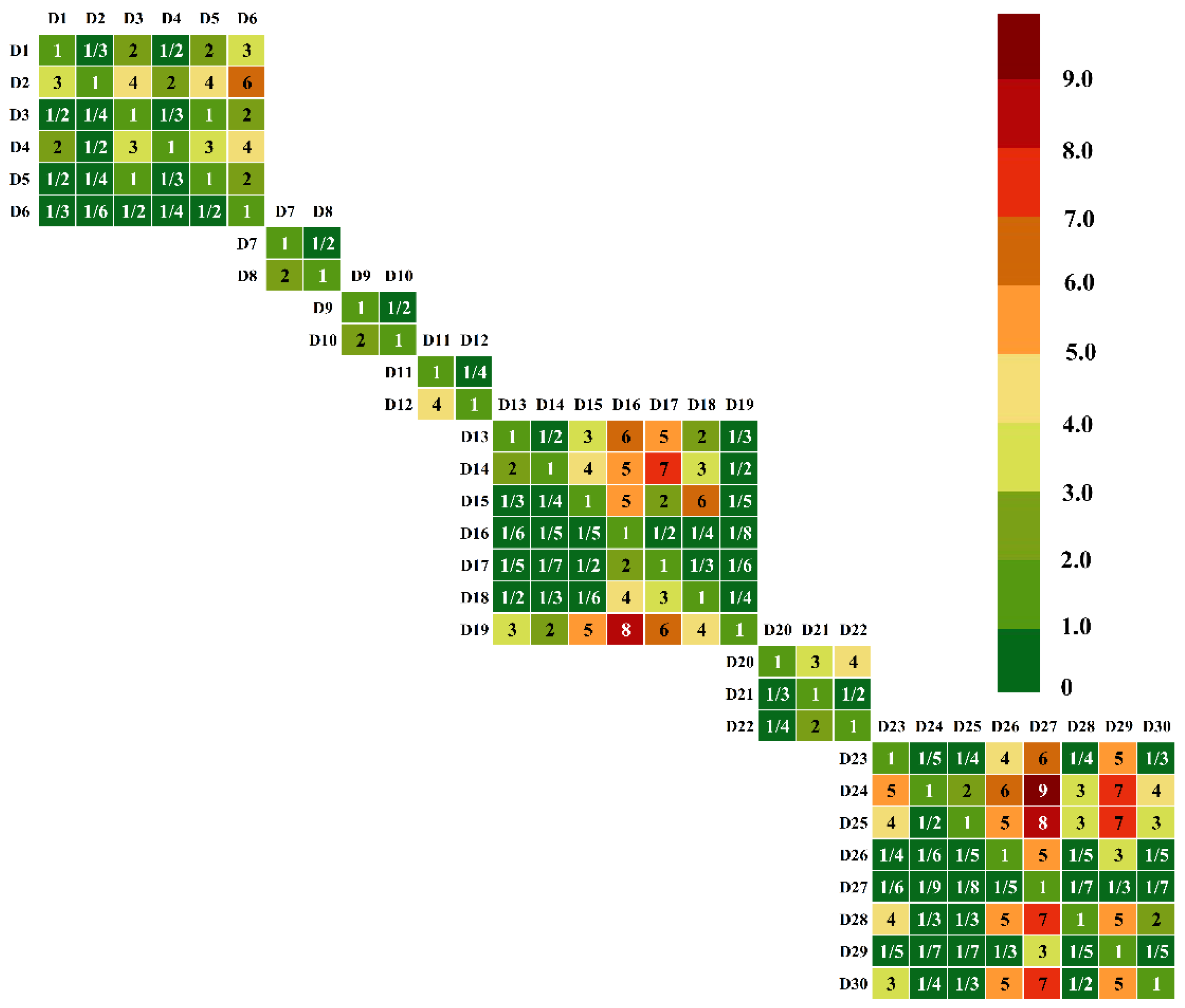
A judgment matrix for indicators C1–C7 was constructed as shown in Figure 4.
By checking the consistency of the matrix, the maximum eigenvalue λmax and the consistency index CI of each matrix was calculated (Table 2). All the matrices with CR < 0.1 were considered to be consistent [24].
Each indicator’s weight value was calculated based on the above results, and the new results are shown in Figure 5 and Figure 6.
The weight ratio of each factor is plotted in Figure 6. The closer the color is to red, the more important the vertical indicator is relative to the indicator on the horizontal axis. For example, the greatest weight ratio in the figure is that of irrigation technology (D24) to water metering facility (D27). A larger proportion of dark green grid blocks corresponding to the horizontal axis index indicates a greater weight in the entire index system.
As can be seen from Figure 5 and Figure 6, human factors (B2) have a more significant impact on the effective utilization coefficient of irrigation water compared to other factors, such as irrigation area scale (D13), irrigation technology (D24), organization degree (D25), crops (D20), water price management (D28), local economic level (D30), and channel anti-seepage ratio (D19). This explains the high effective utilization coefficient of irrigation water in large-scale irrigation areas compared to that of medium-sized irrigation areas.
3.2. Prediction of Effective Utilization Coefficient of Irrigation Water
3.2.1. Predictive Model Establishment
We established a dynamic time series based on the effective utilization coefficients of irrigation water in the irrigation districts of the Shihezi City from 2014 to 2019 The dynamic values are shown in Table 3.
By accumulating each original sequence once, we got
By establishing the corresponding differential equation of the one-variable first-order dynamic model GM (1,1), we obtained the parameters a and b, and established the corresponding grey GM (1,1) prediction model. The grey models of the effective utilization coefficient of irrigation water for all irrigation areas, large-scale irrigation districts, medium-sized irrigation districts, and pure well irrigation districts from 2014 to 2019 were as follows:
3.2.2. Predictive Model Accuracy Test
Residual test:
The residual values of each type of irrigation area are shown in Figure 6. The residual values were randomly distributed around 0, and the range of change was within ±0.0045.
The relative error was obtained by:
The relative errors ε(k) and the relative error values of each type of irrigation area are shown in Figure 7 and Figure 8, respectively.
Average relative error , GM (1,1) model accuracy , and the average relative error of various types of irrigation areas are shown in Table 4.
Table 4 shows that values were all less than 0.01, and the accuracy of the GM (1,1) model of each type of irrigation area was greater than 99%, which meets the accuracy requirement.
3.2.3. Relevance Test of the Predictive Model
Correlation tests estimate the closeness of the shape of the original data series curve to the shape of the model curve. We set , , correlation coefficient , and correlation degree . The correlation coefficients (η(k)) of various types of irrigation areas are shown in Table 5.
4. Discussion
4.1. Analysis of Main Influencing Factors
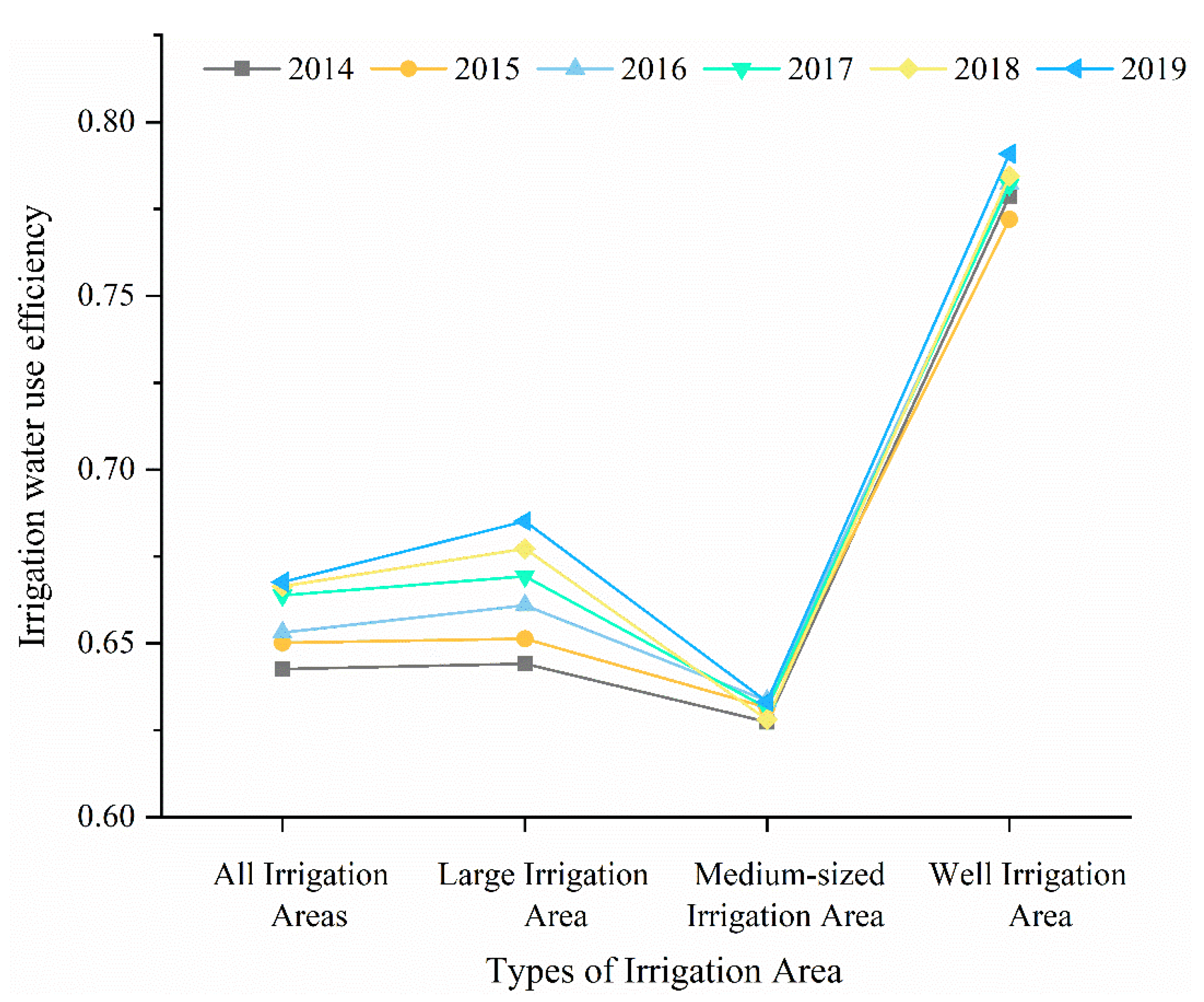
Figure 9 shows that the effective utilization coefficient of irrigation water in the large-scale irrigation area was larger and had a higher annual increase rate than that of the medium-sized irrigation area. This may be due to many factors, such as the decayed channels, the irrigation system, and the ability of farmers in terms of the irrigation piloting. Hence, the irrigation management plays a paramount role in the technology process [25]. In addition, by combining the results in Figure 5, it is evident that uncontrollable factors such as natural conditions, irrigation technology, organization degree, crop types, water price management, local economic level, and channel antiseepage ratio were are all more significant in the large-scale irrigation area. Therefore, the earlier conclusion that irrigation water’s effective utilization coefficient is low if the irrigation area is large is not acceptable. Since more than 90% of the irrigated land in this study area used drip irrigation under mulch to grow cotton, and the economic level of the different irrigation areas did not vary widely, in the following sections we focus on organization degree, water price management, channel antiseepage ratio, and supporting facilities.
4.1.1. Organization Degree
There were 1276 grassroots water conservancy-related personnel in the large-scale irrigation area in the study area, and only 89 personnel in the medium-sized irrigation area. The total irrigated area of the large-scale irrigation area was 2520 km2 and that of the medium-sized irrigation area was 220 km2.
It can be seen from Figure 10 that the number of personnel involved in grassroots water conservancy per unit area in large-scale irrigation areas is greater than that in medium-sized irrigation areas. Field investigations confirmed that there were more technical personnel with higher education and comprehensive quality among the grassroots water conservancy personnel in large-scale irrigation areas than those in medium-sized irrigation areas. Based on sample data of 432 wheat farmers in northwestern China, the results of the Tobit regression analysis also showed that the farmer’s age, income, education level tended to affect the degree of irrigation water efficiency positively [26]. For large-scale irrigation areas, the division of water conservancy management was clearer, and water distribution plans were more effective. Chebil, et al. [27] also found that results of the Tobit analysis showed a positive effect of membership in water users’ associations and experience on water use efficiency. When the irrigation area management personnel are well configured and the management funds are appropriately deployed, water can be carefully dispatched and rationally allocated in the irrigation district, thereby reducing the wastage of water resources caused by dripping and leaks in the water delivery process and improving the effective utilization coefficient of farmland irrigation.
Furthermore, large-scale irrigation districts organized more training sessions for relevant departments, irrigation district managers, water use organizations, and water organizations than medium-sized irrigation districts, which strengthened the public’s awareness of water conservation and created a better social atmosphere for the efficient use of water resources.
4.1.2. Water Price Management
The regulation of water prices can play a unique economic leverage role and promote water conservation and optimal allocation of water resources. There is a strong correlation between the irrigation water utilization coefficient and the price of agricultural water supply. If the water supply price is higher, the irrigation water utilization coefficient is also relatively higher. Chang and Liu [28] found that as the price of irrigation water in the Shanxi Province increased by 10%, its demand decreased by 2.3–6.1%. Mao [29] studied the Yellow River Basin and found that when the price of agricultural irrigation water increased by 10%, the water consumption per agricultural unit area decreased by 5.71–7.41%. Research on the relationship between the price of irrigation water and water consumption in arid oasis areas by Jiang [30] showed that for every 1% increase in irrigation water price, the water demand decreased by 0.31%. The water price directly affects the gross utilization of irrigation water. If the water conservation awareness of farmers can be strengthened through the implementation of precise subsidies and incentive mechanisms, then they can understand the benefits of proper irrigation and the importance of water economizing to create positive effects on the efficient of irrigation water [31], and the effective utilization coefficient of irrigation water can improve.
4.1.3. Channel Antiseepage Ratio
The quality of channel engineering directly affects the effective utilization rate of irrigation water. The channel conditions made a significant impact on irrigation water-use efficiency [26]. A better channel engineering condition leads to a higher utilization rate of irrigation water. Therefore, increasing the lining rate is an important measure to increase irrigation water’s effective utilization factor. As some studies have shown [26], canal seepage prevention in large-scale irrigation areas can increase the canal water utilization coefficient by 0.2–0.4 and reduce channel leakage loss by 50–90%. In terms of reducing leakage loss, low-pressure pipelines have the best water delivery effect. Compared with soil channels, they can reduce leakage loss by 95%, followed by concrete lining that reduces leakage loss by nearly 90%.
In this study, the effective utilization coefficient of irrigation water in the large-scale irrigation area was higher than that in the medium-sized irrigation area. This observation is different from that in previous reports. However, through actual measurements, it was found that the effective use coefficient of field water in each type of irrigation area was approximately 90%. Most of the water loss occurred in the channels. Figure 11 shows the antiseepage ratio of channels in various types of irrigation areas. More than half of the channels in large-scale irrigation areas are lined with concrete, while approximately two-thirds of medium-sized irrigation areas use soil irrigation channels. Lining canal systems reduces the leakage of channel water, improves the channel’s antiscouring ability, reduces the roughness of the channel system, increases the flow, improves the channel’s water delivery and silt removal capacities, expands irrigation water sources, and reduces groundwater replenishment caused by channel leakage. Canals that have been improved by various engineering and technical measures have a canal water utilization coefficient as high as 0.83–0.92, which can save 25–40% of water compared with soil canal irrigation. These factors cause the effective utilization coefficient of irrigation water in large-scale irrigation areas to be higher than that of medium-sized irrigation areas. This finding is consistent with Cui and Zheng’s [32] view that channel length and seepage prevention rate are the main reasons for the difference in channel water utilization coefficient.
Canal lining is also conducive to controlling groundwater level, preventing land salinization, reducing channel siltation, preventing weeds from growing in the channel, saving dredging labor and maintenance costs, and reducing irrigation costs [33].
4.1.4. Supporting Facilities
Since 2014, the effective utilization coefficient of irrigation water at different scales has increased steadily in irrigated areas. The slight change in the coefficient of medium-sized irrigation districts is related to lower investments. The greater increase of the coefficient in large-scale irrigation districts, in 2016, is due to the gradual increase in irrigation district engineering matching rate, channel lining rate, improvement of irrigation district management level, and promotion of water-saving control irrigation technology. By comparing the fixed assets of large-scale irrigation areas and medium-sized irrigation areas (Table 6), it was found that the infrastructure investment in large-scale irrigation areas was much higher than that in medium-sized irrigation areas. This is another reason for the higher effective utilization coefficient of irrigation water in large-scale irrigation areas.
In recent years, some construction projects have been carried out in large- and medium-sized irrigation districts; however, they are still in the initial stage, the supporting infrastructure is not perfect, and there is a lack of information technology-related personnel. In the future, even if the development and implementation of smart irrigation in each type of irrigation area reaches the same level, the level of relevant technical personnel will vary, and there will be differences in water-use efficiency.
4.2. Variation in Effective Utilization Coefficient of Irrigation Water
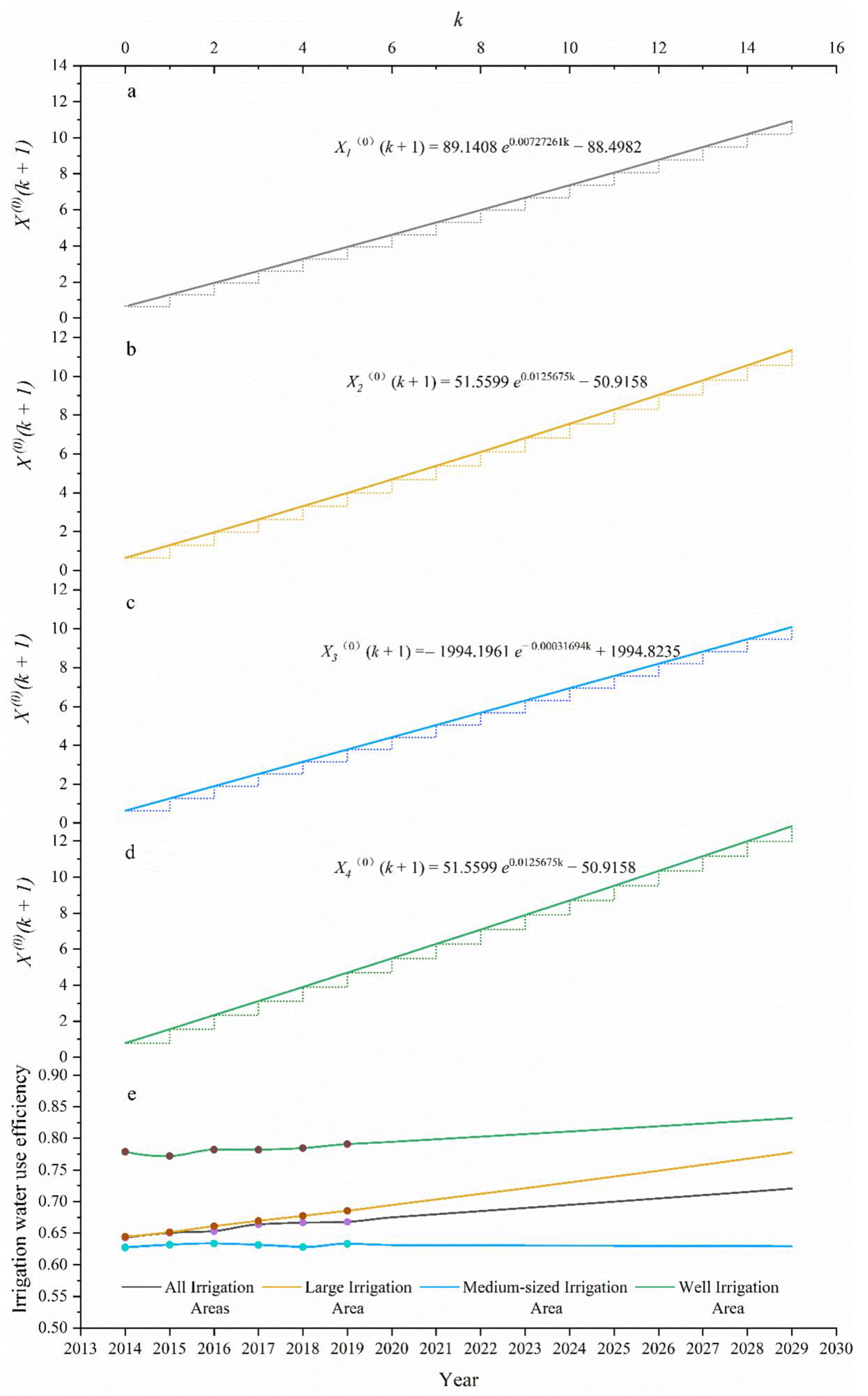
The grey models (Equations (17)–(20)) of the effective utilization coefficients of irrigation water for large-scale, medium-sized, and well-irrigated areas from 2014 to 2019 are shown in Figure 12a–d. Starting from 2020, and were extrapolated to draw Figure 12e, and the effective utilization coefficient of irrigation water for each type of irrigation area for the next ten years was obtained.
According to the development of natural conditions and management models at this stage, the effective utilization coefficient of irrigation water in well irrigation districts and medium-sized irrigation districts will stabilize in the next ten years, while the growth of large-scale irrigation districts will be more significant, with the coefficient reaching 0.7775 in 2029. More than 90% of the irrigated area of the entire study area has had an overall increase in the effective utilization coefficient of irrigation, which can be increased further to 0.7204 in ten years, which is close to the level in developed countries.
5. Conclusions
This study used the analytic hierarchy process and grey model to analyze the influencing factors of the effective utilization coefficient of irrigation water in typical arid and semi-arid areas where drip irrigation has been adopted. It was found that the presumption of larger irrigation areas exhibiting smaller utilization coefficients of irrigation water is not correct. We have shown that in addition to uncontrollable natural conditions, factors such as irrigation technology, completeness of organization, crop types, water price management, local economic level, and channel seepage prevention rate have a significant impact on the effective utilization coefficient of irrigation water. According to the current development model, the utilization coefficient of irrigation water in all irrigation areas will increase continuously. By 2029, the effective utilization coefficient of irrigation water will reach 0.7204, which is close to the level of developed countries. The market plays a decisive role in the allocation of water resources, and hence, improving the water price formation mechanism could be a core comprehensive reform to improve the utilization of agricultural water.
Author Contributions
Investigation, T.H., J.W., and L.Y.; methodology, X.H.; software, L.Y.; formal analysis, L.Y.; writing—original draft preparation, L.Y.; writing—review and editing, G.Y.; visualization, X.G.; project administration, X.H.; funding acquisition, X.H.; All authors have read and agreed to the published version of the manuscript.
Funding
National Natural Science Foundation of China (U1803244, 51969027), Key Technologies R&D Program of Xinjiang Production and Construction Corps (2018AB027), and the Significant Science and Technology Project of Xinjiang Production and Construction Corps (2017AA002).
Institutional Review Board Statement
Not applicable.
Informed Consent Statement
Not applicable.
Data Availability Statement
Not applicable.
Conflicts of Interest
The authors declare no conflict of interest.
References
- Connor, R.; Ortigara, A.; Koncagül, E.; Uhlenbrook, S.; Lamizana-Diallo, B.M.; Zadeh, S.M.; Qadir, M.; Kjellén, M.; Sjödin, J.; Hendry, S.; et al. The United Nations World Water Development Report 2017. Wastewater: The Untapped Resource; United Nations Educational, Scientific and Cultural Organization: Paris, France, 2017. [Google Scholar]
- FAO. Coping with Water Scarcity: An Action Framework for Agriculture and Food Security; Food and Agriculture Organization of the United Nations: Rome, Italy, 2012. [Google Scholar]
- FAO. Water for Sustainable Food and Agriculture; Food and Agriculture Organization of the United Nations: Rome, Italy, 2017. [Google Scholar]
- Hamdy, A.; Ragab, R.; Elisa, S.M. Coping with water scarcity: Water saving and increasing water productivity. Irrig. Drain. 2003, 52, 3–20. [Google Scholar] [CrossRef]
- Haie, N. Transparent Water Management Theory; Springer Nature Singapore Pte Ltd.: Singapore, 2020; pp. 39–70. [Google Scholar]
- Hussain, I.; Turral, H.; Molden, D.; Ahmad, M.-U.-D. Measuring and enhancing the value of agricultural water in irrigated river basins. Irrig. Sci. 2007, 25, 263–282. [Google Scholar] [CrossRef]
- Rodríguez-Díaz, J.A.; Camacho-Poyato, E.; López-Luque, R.; Pérez-Urrestarazu, L. Benchmarking and multivariate data analysis techniques for improving the efficiency of irrigation districts: An application in Spain. Agric. Syst. 2008, 96, 250–259. [Google Scholar] [CrossRef]
- Xiong, J.; Cui, Y.L.; Xie, X.H. Spatial distribution of irrigation water use efficiency and its isogram. J. Irrig. Drain. 2008, 27, 1–5. [Google Scholar]
- Xu, J.Z.; Zhao, J.C.; Gao, F.; Huang, X.Q. Problems with traditional measurement methods of irrigated water use coefficient and its affected factor analysis. China Water Resour. 2004, 17, 39–41. [Google Scholar]
- Liu, C.C.; Zhu, W.; Pang, Y.; Li, X.P.; Gao, F.; Feng, B.Q. Analysis on the key factor of irrigation water use efficiency in different districts. J. Irrig. Drain. 2013, 32, 40–43. [Google Scholar]
- Qin, C.H.; Zhao, Y.; Li, H.H.; Qu, J.L. Assessment of regional water saving potential. South-to-North Water Transfers. Water Sci. Technol. 2020, 20, 1–11. [Google Scholar]
- Kijne, J.W.; Barker, R.; Molden, D. Water Productivity in Agriculture: Limits and Opportunities for Improvement; CABI Publishing and IWMI: Cambridge, CO, USA, 2003. [Google Scholar]
- Li, G.; Zhang, Y.P.; Ban, Y.G. Development status and application prospect of submembrane drip irrigation technology. Xinjiang Water Resour. 2004, Z1, 25–28. [Google Scholar]
- NBS Statistical Yearbook of China; China Statistics Press: Beijing, China, 2019.
- Geng, X.H.; Zhang, X.H.; Song, Y.L. Measurement of irrigation water efficiency and analysis of influential factors: An empirical study based on stochastic production frontier and cotton farmers’ data in Xinjiang. J. Nat. Resour. 2016, 6, 1–13. [Google Scholar]
- Wei, L.L.; Li, W.M. Agricultural water use efficiency and influencing factors in Xinjiang. J. Xinjiang Univ. 2014, 42, 7–10. [Google Scholar]
- Xu, D.W. Calculation and analysis of effective utilization coefficient of farmland irrigation water in Huaibei plain area. Harnessing Huaihe River 2020, 20, 16–18. [Google Scholar]
- Guan, S.P.; Liu, F.P.; Jin, W.R. An analysis of the influence factors on the effective utilization coefficient of irrigation water in Jiangxi Province. China Rural Water Hydropower 2017, 11, 104–106, 110. [Google Scholar]
- Wu, W.W. Calculation and analysis of effective utilization coefficient of farmland irrigation water in Jinzhong city in 2019. China Water Transp. 2020, 20, 170–172. [Google Scholar]
- Liu, T.; Zhang, Q.N. Calculation and analysis of effective utilization coefficient of farmland irrigation water in Ningbo. China Water Resour. 2020, 11, 27–29. [Google Scholar]
- Zhang, L.; Zhang, H.L. Calculation and evaluation on coefficient of irrigated water use in Ningxia in 2016. China Water Resour. 2017, 11, 21–24. [Google Scholar]
- Wang, J.S.; Dang, S.Z.; Li, H.X.; Chen, D. Study on the Utilization Coefficient of Irrigation Water of Ningxia. Yellow River 2014, 36, 82–84, 89. [Google Scholar]
- Saaty, W.; Thomas, L. Marketing applications of the analytic hierarchy process. Manag. Sci. 1980, 26, 641–658. [Google Scholar]
- Deng, J.L. The relational space in grey system theory. Fuzzy Math. 1985, 1, 1–10. [Google Scholar]
- Chemak, F. The Water Demand Management by Monitoring the Technology Performance and the Water Use Efficiency. Am. J. Environ. Sci. 2012, 8, 241–247. [Google Scholar]
- Wang, X.Y. Irrigation Water Use Efficiency of Farmers and Its Determinants: Evidence from a Survey in Northwestern China. Agric. Sci. China 2010, 9, 1326–1337. [Google Scholar] [CrossRef]
- Chebil, A.; Abbas, K.; Frija, A. Water Use Efficiency in Irrigated Wheat Production Systems in Central Tunisia: A Stochastic Data Envelopment Approach. J. Agric. Sci. 2014, 6, 63–71. [Google Scholar] [CrossRef]
- Chang, M.Q.; Liu, J.P. Analysis of relation between agricultural water supply price and demand. Water Resour. Dev. Res. 2005, 5, 21–24, 42. [Google Scholar]
- Mao, C.M. Analysis of the Relationship between Agricultural Water Price Reform and Water-Saving Effect. China Rural Water Hydropower 2005, 4, 3–5. [Google Scholar]
- Jiang, Y.; Wang, X.F. Research on the Relationship between Irrigation Water Price and Irrigation Water in Drought Oases. China Rural Water Hydropower 2009, 5, 161–163. [Google Scholar]
- Delavar, A.; Yavari, G.; Javid, M.A.; Fadaei, M.S. Evaluating Effective Factors on Water Use Efficiency Resources in Wheat. Int. J. Resist. Econ. 2015, 3, 17–26. [Google Scholar]
- Cui, Y.L.; Tan, F.; Zheng, C.J. Analysis of irrigation efficiency and water saving potential at different scales. Adv. Int. Water Sci. 2010, 21, 788–794. [Google Scholar]
- He, W.Q.; Liu, Q.C. The Present Development Status and Trends of Canal Lining and Seepage Control Techniques in China. China Rural Water Hydropower 2009, 6, 3–6. [Google Scholar]
Figure 1.
The study area is an oasis agroecosystem in the Manas River Basin (b) in Xinjiang, located in the northwest of China (a), and includes 8 irrigation areas. All typical field locations are shown in (c).
Figure 1.
The study area is an oasis agroecosystem in the Manas River Basin (b) in Xinjiang, located in the northwest of China (a), and includes 8 irrigation areas. All typical field locations are shown in (c).
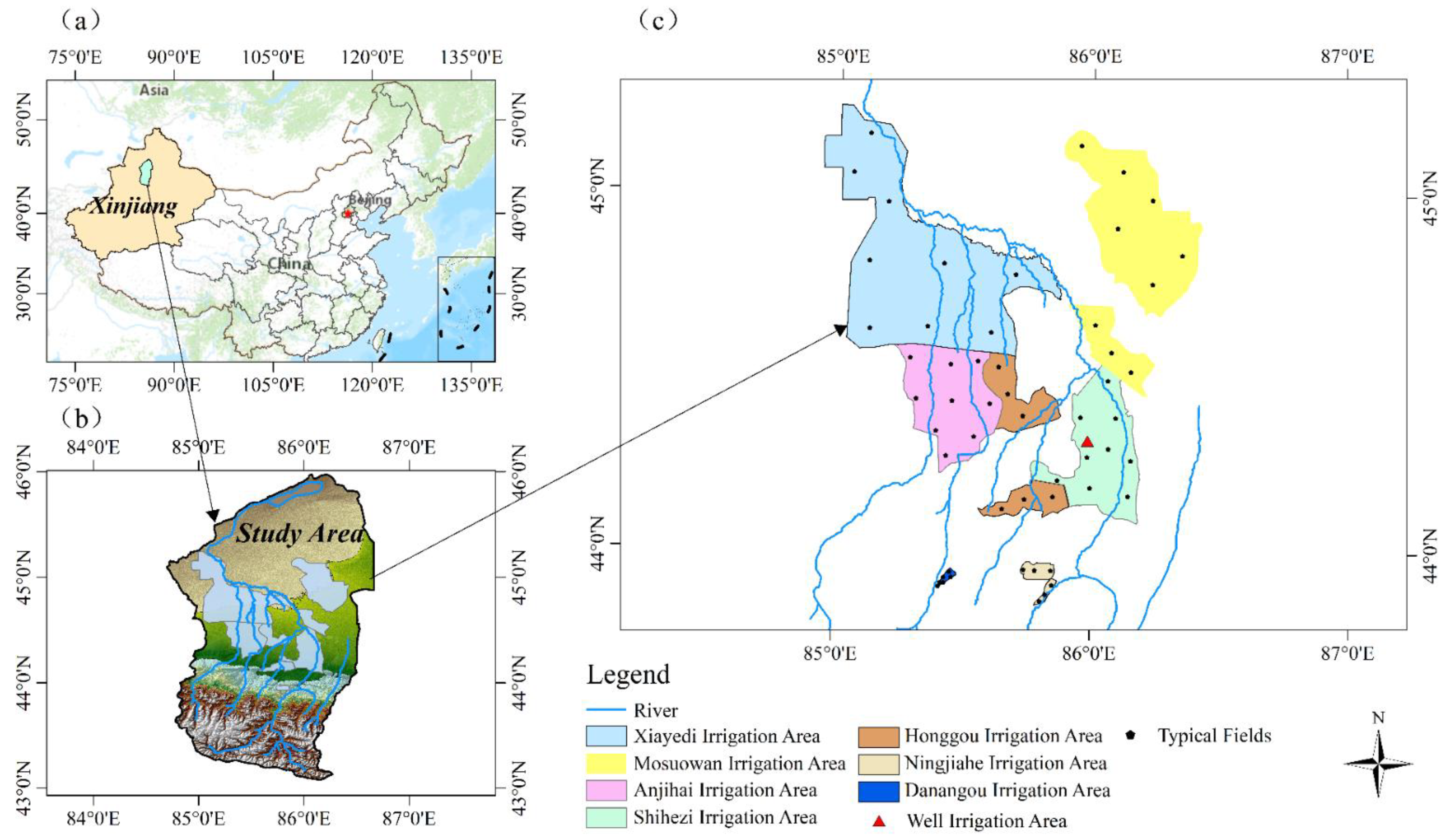
Figure 2.
The water path of irrigation system in the study area.
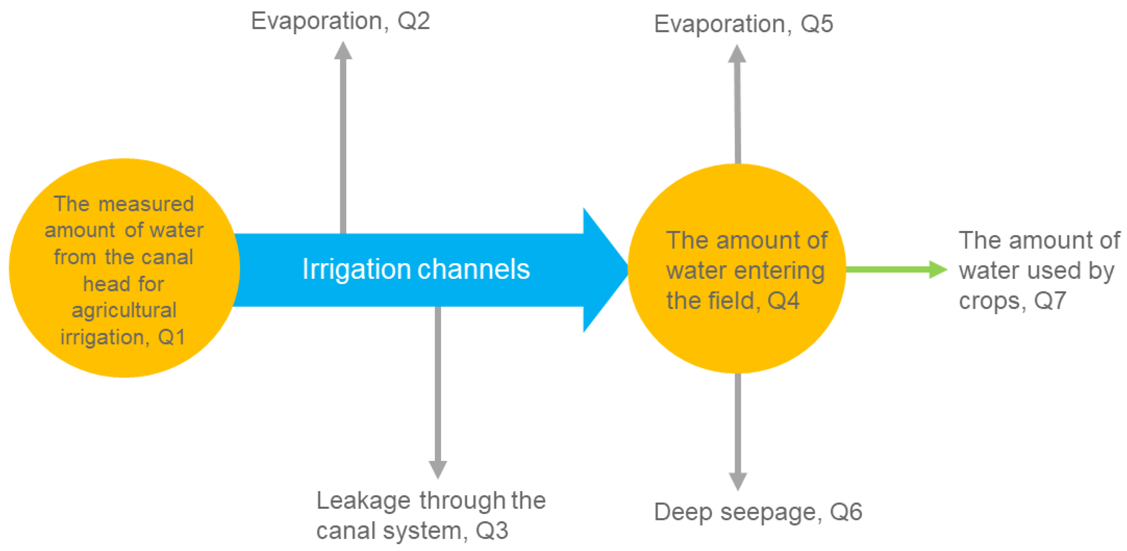
Figure 3.
Framework of the evaluation index system for the effective utilization coefficient of irrigation water.
Figure 3.
Framework of the evaluation index system for the effective utilization coefficient of irrigation water.
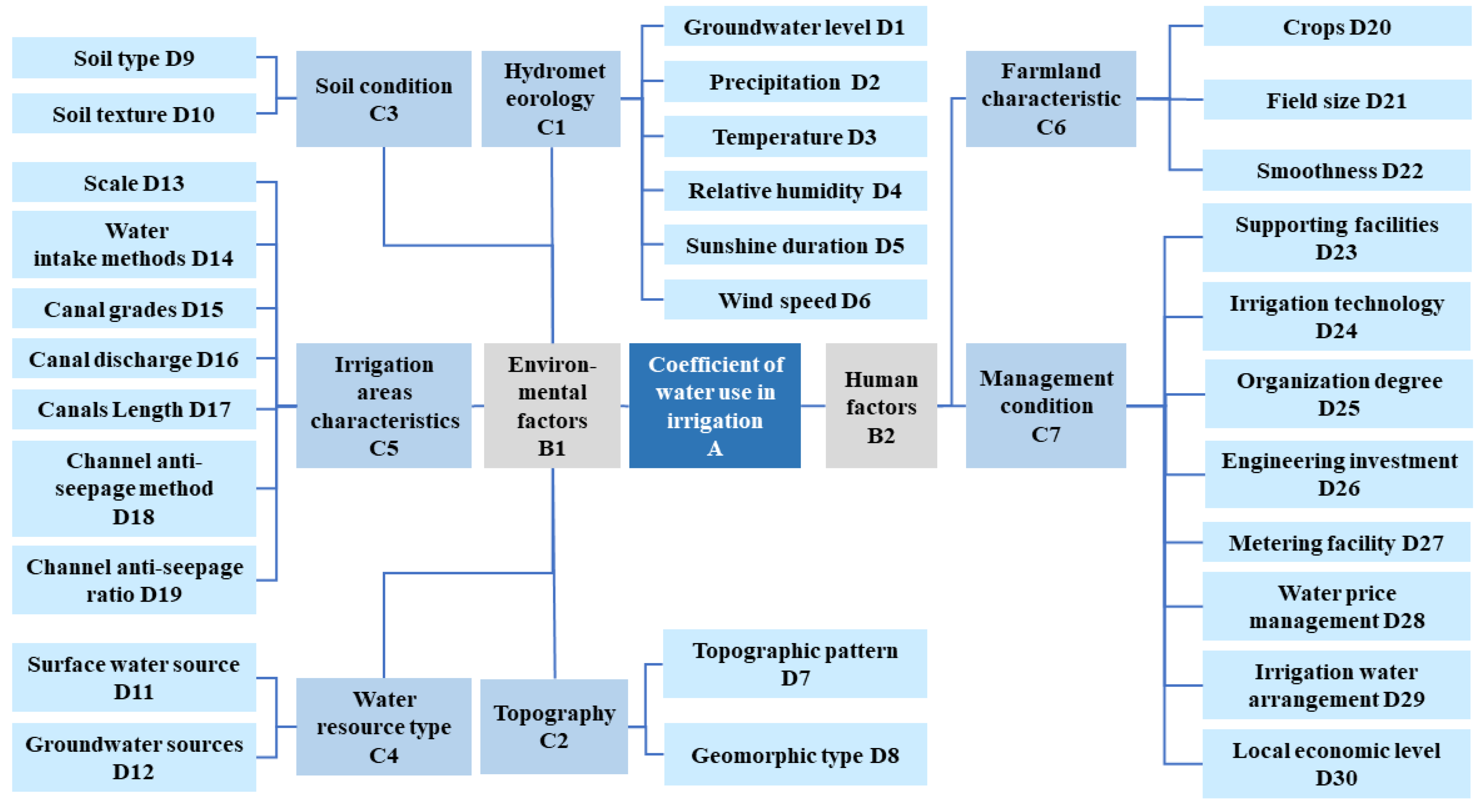
Figure 4.
C1–C7 judgment matrix constructed by the analytic hierarchy process method.

Figure 5.
Weight values of all indices affecting the effective utilization coefficient of irrigation water.
Figure 5.
Weight values of all indices affecting the effective utilization coefficient of irrigation water.
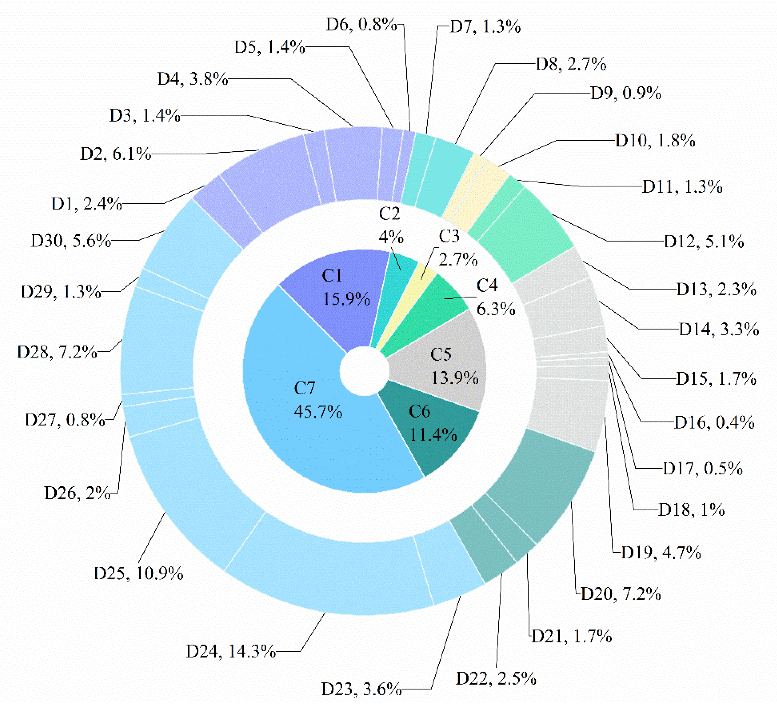
Figure 6.
Weight ratio of all evaluation indices of the effective utilization coefficient of irrigation water.
Figure 6.
Weight ratio of all evaluation indices of the effective utilization coefficient of irrigation water.
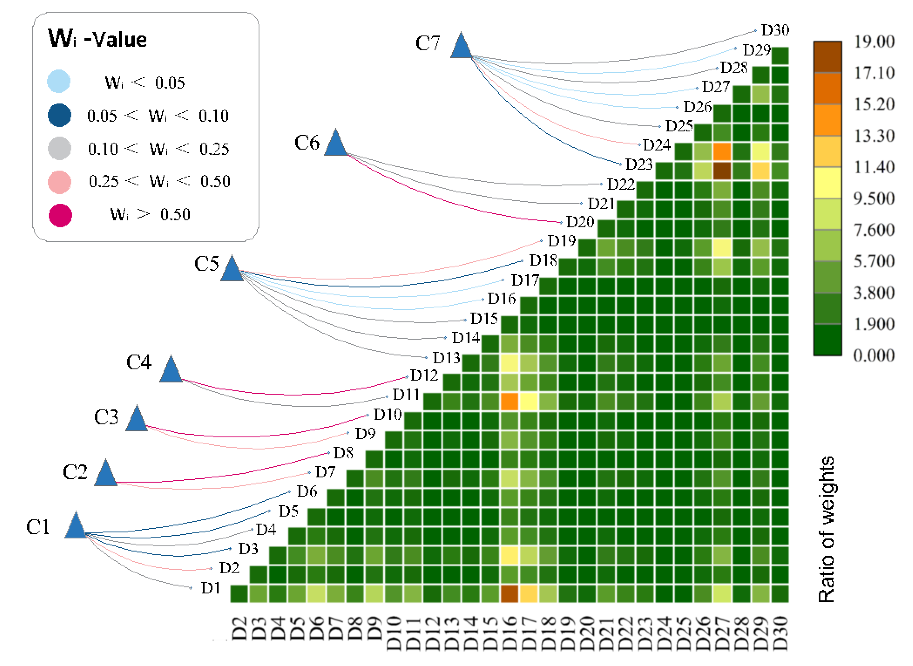
Figure 7.
Residuals of various types of irrigation areas .
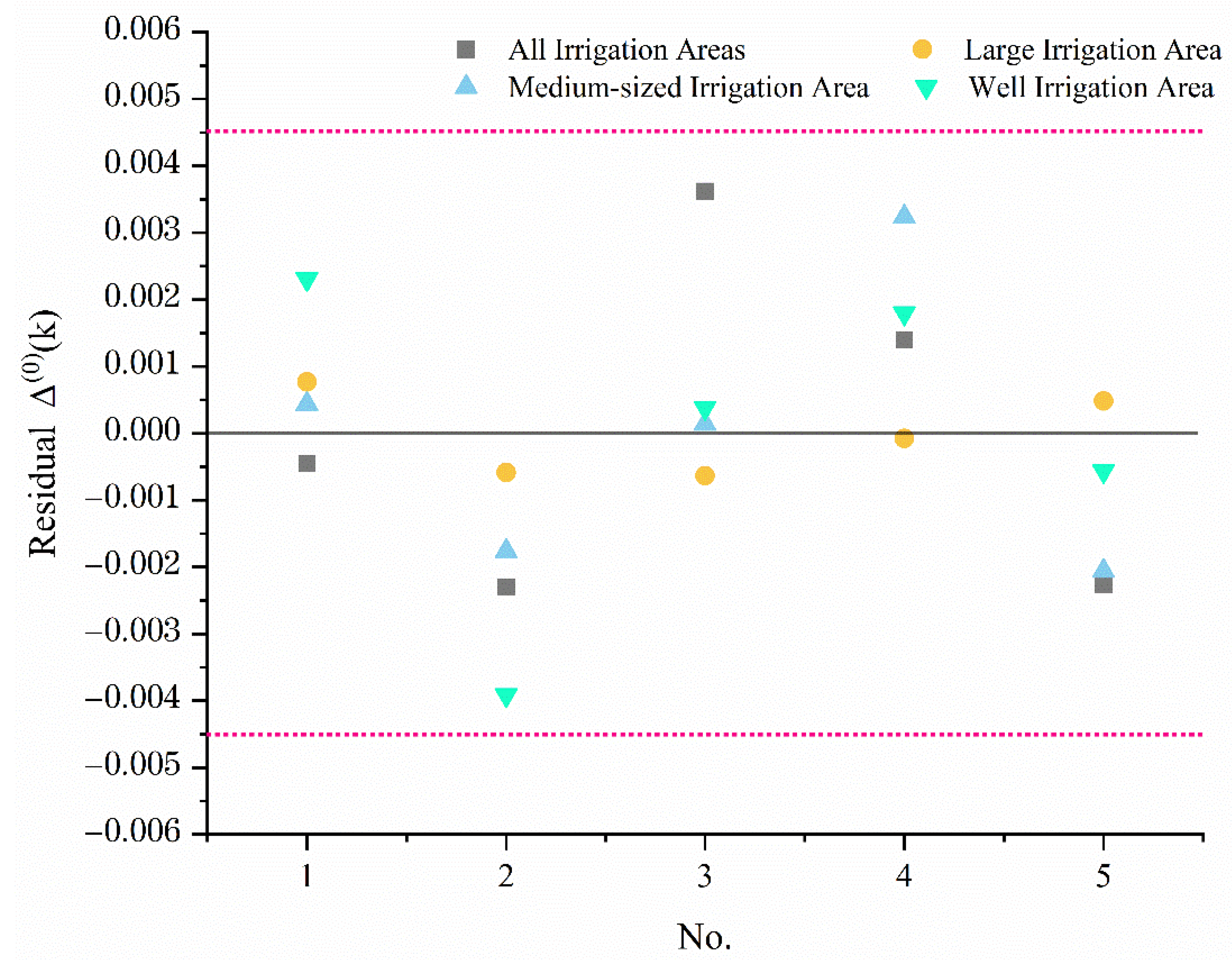
Figure 8.
Relative error values of various types of irrigation areas.
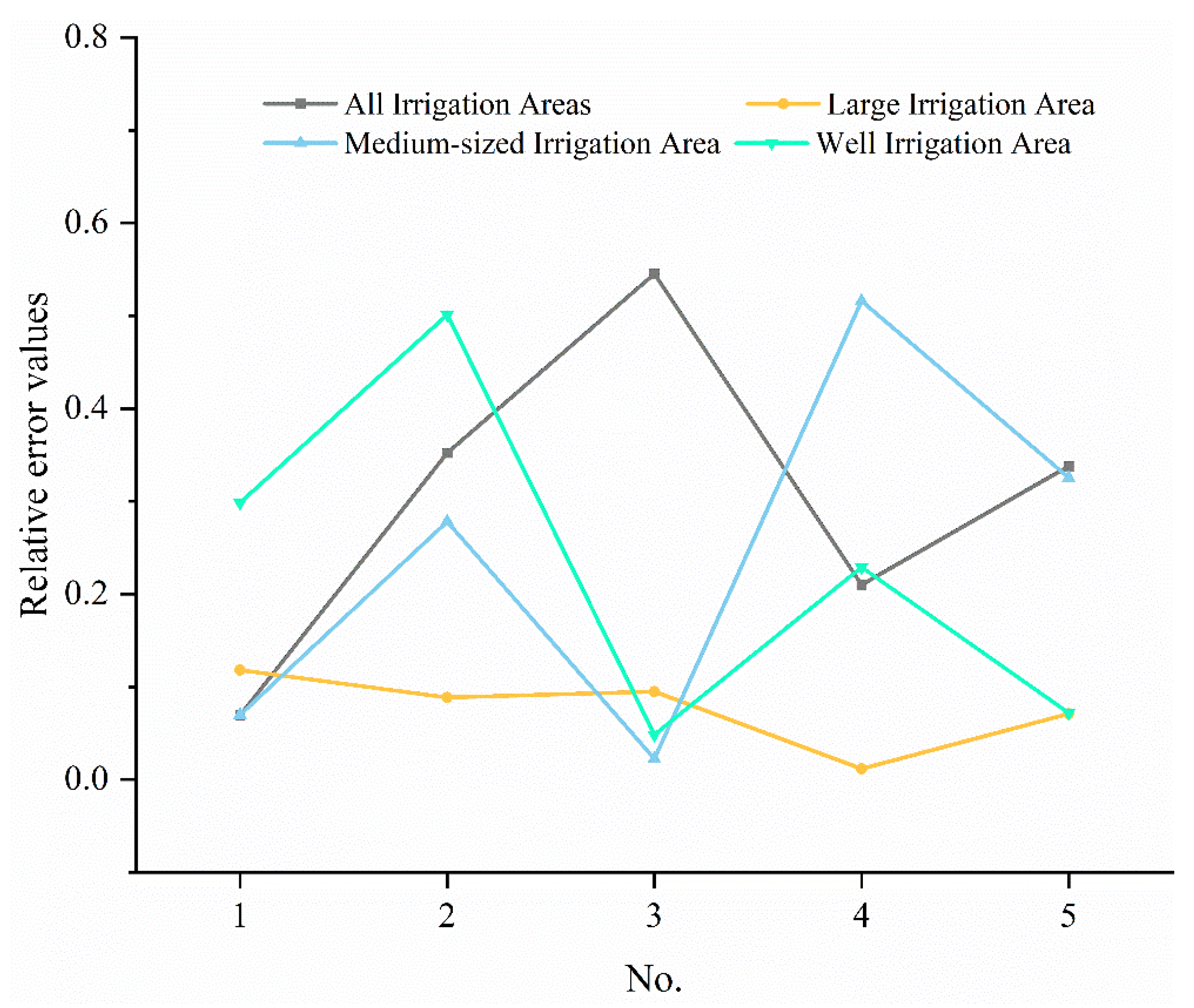
Figure 9.
Effective utilization coefficient of irrigation water in various types of irrigation areas from 2014 to 2019.
Figure 9.
Effective utilization coefficient of irrigation water in various types of irrigation areas from 2014 to 2019.

Figure 10.
The number of grassroots water conservancy-related personnel and irrigated area in different types of irrigation areas.
Figure 10.
The number of grassroots water conservancy-related personnel and irrigated area in different types of irrigation areas.
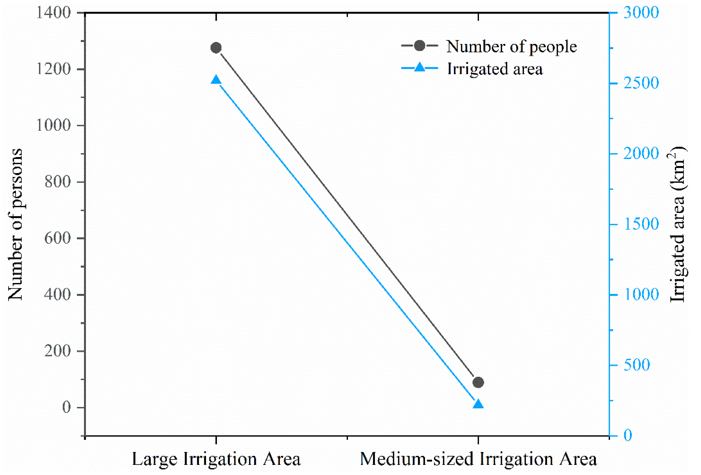
Figure 11.
Canal seepage prevention ratios of for large- and medium-scaled irrigation areas.
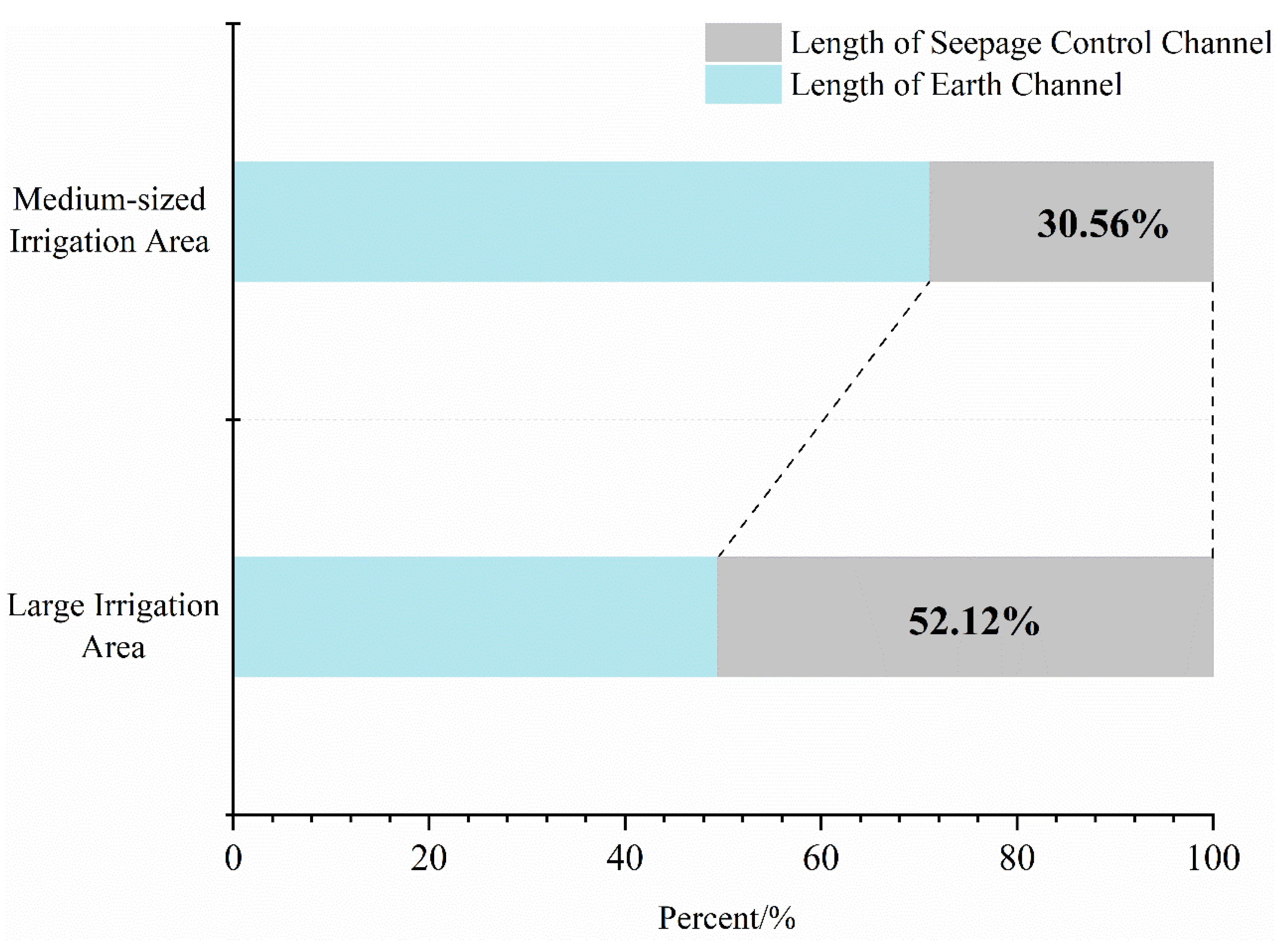
Figure 12.
Changes in the effective utilization coefficient of irrigation water in different types of irrigation areas (grey model curves for (a) all irrigation areas, (b) large irrigation areas, (c) medium-sized irrigation areas, and (d) well irrigation areas in the next 10 years; (e). variations in various types of irrigation areas from 2014 to 2029.


Table 1.
Matrix consistency judgment index table.
| n | 1 | 2 | 3 | 4 | 5 | 6 | 7 | 8 | 9 |
|---|---|---|---|---|---|---|---|---|---|
| RI | 0.00 | 0.00 | 0.58 | 0.90 | 1.12 | 1.24 | 1.32 | 1.41 | 1.45 |
Table 2.
C1–C7 consistency test results.
| C | λmax | CI | CR |
|---|---|---|---|
| C1 | 6.0551 | 0.0110 | 0.0089 |
| C2 | 2.0000 | 0.0000 | - |
| C3 | 2.0000 | 0.0000 | - |
| C4 | 2.0000 | 0.0732 | - |
| C5 | 7.7551 | 0.1259 | 0.0953 |
| C6 | 3.1078 | 0.0539 | 0.0929 |
| C7 | 8.8240 | 0.1177 | 0.0835 |
Table 3.
Effective utilization coefficient of irrigation water for irrigation areas in the study area during 2014–2019.
Table 3.
Effective utilization coefficient of irrigation water for irrigation areas in the study area during 2014–2019.
| No | Year | All Irrigation Areas | Large Irrigation Area | Medium-Sized Irrigation Area | Well Irrigation Area |
|---|---|---|---|---|---|
| 1 | 2014 | 0.6426 | 0.6441 | 0.6274 | 0.7788 |
| 2 | 2015 | 0.6502 | 0.6513 | 0.6315 | 0.7720 |
| 3 | 2016 | 0.6531 | 0.6609 | 0.6335 | 0.7822 |
| 4 | 2017 | 0.6638 | 0.6693 | 0.6314 | 0.7819 |
| 5 | 2018 | 0.6664 | 0.6772 | 0.6281 | 0.7845 |
| 6 | 2019 | 0.6676 | 0.6852 | 0.6332 | 0.7909 |
Table 4.
Average relative error and model accuracy of various types of irrigation areas.
| Irrigation Area Type | All Irrigation Areas | Large Irrigation Area | Medium-Sized Irrigation Area | Well Irrigation Area |
|---|---|---|---|---|
| 0.00000284 | −0.00000894 | −0.00000001 | 0.00000171 | |
| 0.3027 | 0.0767 | 0.2422 | 0.2297 | |
| 99.6973 | 99.9233 | 99.7578 | 99.7703 |
Table 5.
Correlation coefficient and correlation degree r for various types of irrigation areas.
| No | All Irrigation Areas | Large Irrigation Area | Medium-Sized Irrigation Area | Well Irrigation Area |
|---|---|---|---|---|
| 1 | 1.4206 | 0.5272 | 0.9009 | 0.6459 |
| 2 | 0.7810 | 0.6026 | 0.6277 | 0.4980 |
| 3 | 0.5911 | 0.5803 | 1.0000 | 1.0000 |
| 4 | 1.0000 | 1.0000 | 0.4684 | 0.7125 |
| 5 | 0.7894 | 0.6538 | 0.5872 | 0.9491 |
| r | 0.9164 | 0.6728 | 0.7169 | 0.7611 |
It can be seen from Table 5 that r > 0.6, which meets the requirements.
Table 6.
Original and net value of fixed assets of water conservancy in various types of irrigation areas.
Table 6.
Original and net value of fixed assets of water conservancy in various types of irrigation areas.
| Irrigation Area Type | Large Irrigation Area | Medium-Sized Irrigation Area | ||
|---|---|---|---|---|
| Total (Ten thousand yuan) | Original value of fixed assets | Net value of fixed assets | Original value of fixed assets | Net value of fixed assets |
| 163,499 | 90,614 | 8282 | 6263 | |
Publisher’s Note: MDPI stays neutral with regard to jurisdictional claims in published maps and institutional affiliations. |
© 2021 by the authors. Licensee MDPI, Basel, Switzerland. This article is an open access article distributed under the terms and conditions of the Creative Commons Attribution (CC BY) license (http://creativecommons.org/licenses/by/4.0/).
Share and Cite
MDPI and ACS Style
Yang, L.; Heng, T.; Yang, G.; Gu, X.; Wang, J.; He, X. Analysis of Factors Influencing Effective Utilization Coefficient of Irrigation Water in the Manas River Basin. Water 2021, 13, 189. https://doi.org/10.3390/w13020189
AMA Style
Yang L, Heng T, Yang G, Gu X, Wang J, He X. Analysis of Factors Influencing Effective Utilization Coefficient of Irrigation Water in the Manas River Basin. Water. 2021; 13(2):189. https://doi.org/10.3390/w13020189
Chicago/Turabian StyleYang, Lili, Tong Heng, Guang Yang, Xinchen Gu, Jiaxin Wang, and Xinlin He. 2021. "Analysis of Factors Influencing Effective Utilization Coefficient of Irrigation Water in the Manas River Basin" Water 13, no. 2: 189. https://doi.org/10.3390/w13020189
Note that from the first issue of 2016, this journal uses article numbers instead of page numbers. See further details here.