A Robust Neutrosophic Modeling and Optimization Approach for Integrated Energy-Food-Water Security Nexus Management under Uncertainty


1
Department of Statistics and Operations Research, Aligarh Muslim University, Aligarh 202002, India
2
Indian Statistical Institute, 203 B. T. Road, Kolkata 700108, India
3
Industrial Engineering Department, College of Engineering, King Saud University, P.O. Box 800, Riyadh 11421, Saudi Arabia
4
Department of Statistics and Operations Research, College of Science, King Saud University, P.O. Box 2455, Riyadh 11451, Saudi Arabia
*
Author to whom correspondence should be addressed.
†
Current address: Indian Statistical Institute, 203 B. T. Road, Kolkata 700108, India.
‡
These authors contributed equally to this work.
Water 2021, 13(2), 121; https://doi.org/10.3390/w13020121
Submission received: 28 November 2020
/
Revised: 5 January 2021
/
Accepted: 6 January 2021
/
Published: 7 January 2021
(This article belongs to the Special Issue The Water-Energy-Food Nexus: Sustainable Development)
Abstract
:Natural resources are a boon for human beings, and their conservation for future uses is indispensable. Most importantly, energy-food-water security (EFWS) nexus management is the utmost need of our time. An effective managerial policy for the current distribution and conservation to meet future demand is necessary and challenging. Thus, this paper investigates an interconnected and dynamic EFWS nexus optimization model by considering the socio-economic and environmental objectives with the optimal energy supply, electricity conversion, food production, water resources allocation, and CO emissions control in the multi-period time horizons. Due to real-life complexity, various parameters are taken as intuitionistic fuzzy numbers. A novel method called interactive neutrosophic programming approach (INPA) is suggested to solve the EFWS nexus model. To verify and validate the proposed EFWS model, a synthetic computational study is performed. The obtained solution results are compared with other optimization approaches, and the outcomes are also evaluated with significant practical implications. The study reveals that the food production processes require more water resources than electricity production, although recycled water has not been used for food production purposes. The use of a coal-fired plant is not a prominent electricity conversion source. However, natural gas power plants’ service is also optimally executed with a marginal rate of production. Finally, conclusions and future research are addressed. This current study emphasizes how the proposed EFWS nexus model would be reliable and beneficial in real-world applications and help policy-makers identify, modify, and implement the optimal EFWS nexus policy and strategies for the future conservation of these resources.
1. Introduction
Natural resources are precious and essential for human lives. Primarily, energy, food, and water (EFW) are the basic needs for daily life and human survival. A rapid increase in the population significantly enhances these resources’ demand, causing depreciation and depletion in these resources’ utility rates. As a result, the acquisition and conservation of these resources become indispensable to meet future needs. These resources are inter-related and affect each other, either directly or indirectly. Thus, the inter-dependence nature of EFW resources has been explored as a sort of composite network, called energy-food-water security (EFWS) nexus management. According to the EIA report, [1] in the US, approx. 89% of the electricity was generated by coal and natural-gas-fired power plants, whereas a massive amount of water is consumed for pumping and cooling purposes. Presently, about 1.29 billion people throughout the world are not accessing electricity [2]. To meet such a massive electricity demand, the accumulation of water resources for coal-fired power plants and the fuel extraction process will be challenging. Moreover, population growth is expected to increase concerning food demand, about 53% by 2050 [3]. It compels the need to realize and identify the interactions among various resources requirements to fulfill future demands affecting the EFWS nexus system’s composition.
According to [3]’s report, food production and supply purpose consume approx. 31% of global energy. An increase in the mass population results in higher demand for EFW resources drastically [3]. By 2050, a predictive analysis indicates that the world population will increase by about 49% [4]. Furthermore, it is noticed that integrated EFWS nexus model are complex and dynamic due to not only the inter-dependencies of these three resources that influence each other at various level, but also the involvement of different factors such as economic, social, and environmental, etc. which made it more complicated. Nexus management is gaining more attention due to its prime concerns about energy, food, and water security. It is expected that the proposed EFWS nexus model would be well-enough to address and answer the most critical queries, such as “optimal distribution of resources,” “balancing the trade-off between total economic cost and CO emissions”, “evaluating and designing the policies and necessary initiatives.” Quantitative optimization models are powerful tools in identifying, assessing, and summarizing the critical factors and provides globally acceptable outcomes to facilitate the decisions and relevant processes.
Uncertain parameters are often encountered in the EFWS decision-making model. Unlike fuzzy and random parameters, uncertain parameters are depicted as triangular or trapezoidal intuitionistic fuzzy numbers. A fuzzy parameter only deals with the degree of belongingness (acceptance) of the element into a feasible solution set. It does not consider the degree of non-belongingness (rejections) of the element into the same feasible solution set, an integrated part of the decision-making processes. Furthermore, uncertainty due to randomness is indicated with random parameters. Sometimes, it may not be possible to have historical data for which the random parameters are estimated. According to some specified probability distribution function, the forecasting pattern and parameters estimation of random variables is much dependent on the behavior and nature of the historical data. An intuitionistic fuzzy parameter deals with the degree of belongingness (acceptance) and degree of non-belongingness (rejections) of the element into the same feasible solution set, simultaneously. For example, if the decision maker intends to quantify the cost of transportation with some estimated value, such as transportation cost from water resources zones to electricity conversion plant is 54$, then the most likely estimated interval would be 50–58$, along with some hesitation degree that may be given as 48–60$, which ensures less violation of risks with degree of acceptance and non-acceptance. Also, there is no scope for the historical data while dealing with intuitionistic fuzzy parameters (Ahmad et al. [5]). Thus, the prime motive behind the selection of intuitionistic fuzzy parameters is to avoid the shortcomings of fuzzy vague random parameters. Therefore the quantitative and analytical study of EFWS nexus management network has the utmost need for the time in balancing the equilibrium among optimal resource use, socio-economic and environmental objectives, and designing fruitful policies. Many past studies confront the research domain of EFWS nexus. Still, most of them are confined to either individual resource management fields such as water sector, energy-conversion, agricultural production, or two sectors such as water-energy nexus, particular problems such as water uses, or theoretical and conceptual development of the EFWS nexus. This study has unified all three resources and the socio-economic and environmental objectives at a single platform.
An interactive neutrosophic programming approach (INPA) is developed to solve the proposed EFWS nexus model. The discussed INPA manages indeterminacy or neutral thoughts while making decisions for multiobjective optimization problems. Neutrality is the region of propositions’ values negligence, which exists between truth and falsity degree. Thus, the neutrosophic decision set theory is a more generalized and flexible approach than the fuzzy and intuitionistic fuzzy set theory due to indeterminacy degree. Therefore, the proposed solution approach can also be regarded as a contribution to the optimization technique domain.
The main aim and objective of this paper are to explore and highlight an integrated modeling and optimizing system for EFWS nexus management. A useful quantitative and analytical model would establish the trade-offs among objectives and constraints to achieve the socio-economic demands and environmental impacts while using the energy, food, and water resources. The proposed EFWS model inherently estimates the various costs associated with the limited EFW resources, socio-economic demands, and CO emissions abatement over the multi-period planning horizons. It is also capable of dealing with more generalized uncertainty due to hesitation while depicting the parameters. Various inter-connected components such as production, distribution, and consumption of the EFWS nexus model are quantitatively and analytically examined. The proposed EFWS nexus model’s main advantage can be realized by having it be consistent with and competent compared with real-life management problems. The current study also demonstrates how these resources can be used optimally and how they can be conserved to meet future demand. Practical implications are well addressed based on obtained solution results. Post-optimality analyses are performed to generate and identify the most promising solutions under different risk factors. Therefore, the presented study can help decision-makers design the optimal policies and strategies for EFWS nexus management under uncertainty.
2. Literature Review
Over recent decades, optimal use of resources has made significant impacts in research and development fields to identify, quantify, and analyze the decision-makers’ policies and strategies while managing the Energy-Water-Food nexus management system. The most effective and indispensable modeling texture of the EFWS network under various uncertainties was developed by many authors, practitioners, and researchers. Bieber et al. [6] developed a methodology and outlook for resilient and sustainable supply chain planning in the energy-water-food nexus at the city-region level. Uen et al. [7] proposed a holistic approach for the synergetic management of the Water-Energy-Food nexus and applied NSGA-II to solve the model. Tsolas et al. [8] discussed a novel water-energy nexus optimization and presented a case study at the country and state level. Namany et al. [9] also addressed a resources management-oriented Energy-water-Food nexus optimization model with a real-life application. Gao et al. [10] introduced a water–food–energy nexus management model for minimizing the cost-coal and production-cost of agricultural products. Zhang et al. [11] attempted to develop an assessment-optimization methodology for Water-Energy-Food nexus synergies and concluded water supply as a critical factor in the modeling approach. Li et al. [12] explored the synergies within the Water-Energy-Food nexus system and presented as a case study Shenzhen city using the proposed model. Hamidov and Helming [13] presented a theoretical study on the ever-increasing literature on the WEF nexus management along with concluding remarks. [14] discussed an integrated energy-water-food supply chain optimization model with a case study. Ji et al. [15] addressed a crop-biomass production planning problem with food-energy-water nexus under uncertainties. The developed model assists the decision-makers in adopting adequate policies and strategies. Okola et al. [16] designed a multiobjective optimization framework to highlight the complexity linked with Food-Energy-Water Nexus and suggested the optimal production and resource consumption policies over different planning horizons.
Many researchers discussed their work by incorporating different sorts or forms of uncertainty in the water, energy, and food nexus optimization model as far as uncertainties are concerned. We summarized some recent developments and advanced studies in the uncertainty domain in the EFWS nexus model. Li et al. [17] also developed an integrated agricultural water-energy-food nexus management model under fuzzy demands for the resources and applied to a case study data-set. Li et al. [18] suggested a water-food-energy nexus optimization outlook for irrigated agriculture under dual stochastic uncertainty of available water resources and validated the model based on a real case study. Li et al. [19] addressed the optimization-assessment of energy, food, water, and land framework for bioenergy production in interval-valued uncertainty and demonstrated a case study in northeast China. Yu et al. [20] explored a copula-based fuzzy interval-random programming approach under joint-risk and implemented a real-world case study in Henan Province, China. Elsayed et al. [21] studied a Nile Water-Food-Energy Nexus management system and depicted a trade-offs opportunity among the resources use policies to a case study in Sudan. Tan and Zhang [22] suggested a robust fractional programming approach to address the agricultural water management model under the risk uncertainty and validated using simulations and comparisons with existing alternatives. Hurford [23] also identified and assessed the impacts of water-energy-food security in developing country and concluding remarks are made based on the study. Govindan and Al-Ansari [24] discussed a flexible computational framework for integrated energy-water-food security under risk factors and performed a case study of the agricultural sector in the State of Qatar. Ji et al. [25] developed an inexact hybrid model for food-energy-water nexus management under the mixed-character uncertainties and presented practical implications based on the case study in Shandong, China. Yu et al. [26] propounded an effective water-energy-food nexus planning system, and a multi-level interval fuzzy credibility-constrained programming is suggested to deal with the uncertainties and then implemented on a real-case study in Henan Province. Furthermore, Hang et al. [27] designed the local food, energy and water production system based on the nexus concept. Martinez-Hernandez et al. [28] developed the new software tool for techno-ecological simulation of local food-energy-water systems. Also, an integrated nexus modeling network is scarce in the literature, which can introduce and implement the energy, food, and water resources efficiently. In association with socio-economic objectives, incorporating environmental protections into a robust modeling and optimization framework is also the need for the current state-of-art. The EFWS nexus management perspective is necessary for the quantitative and qualitative study of the complex interconnected network and evaluating the outcomes for optimal policies and development for the whole system.
3. Development of Energy-Food-Water Security Nexus Model
The proposed EFWS model is formulated to optimize and manage the available energy, food, and water nexus resources in intuitionistic fuzzy uncertainty over different periods. The various costs associated with the operations, production, supply, and CO emissions abatement are contemplated over the socio-economic and environmentally oriented objective. The quantity of CO emissions is also a challenging task from the environmental point of view. The severe impact of such toxic emissions affects both flora and fauna. Thus, the developed model integrates and adheres to EFWS nexus management’s essential aspects by undertaking the vague uncertainty among different parameters. The inter-connected component in the proposed EFWS nexus management model is shown in Figure 1, which also signifies the research domain of this study. The useful notions and descriptions used in the proposed EFWS model are depicted in Table 1. The optimal allocation of the energy-supply quantity of coal and natural gas, the available capacity of the power plant to produce electricity, amount of ground and surface water required for food production, the volume of ground, surface, and recycled water needed for electricity production, and socio-economic demands for EFW (Energy, Food and Water) turnover in a well-specified production planning periods are the prime characteristic features of the proposed EFWS model. The first objective is developed to reduce the total economic cost comprising energy-supply costs for electricity production, costs of electricity-production, costs of water-delivery, costs of food production, and finally CO emissions abatement costs over time horizons. The second objective mitigates the CO emissions produced during electricity conversion and food production, respectively. All the related parameters are taken as triangular intuitionistic fuzzy and resolved into their crisp form using a robust ranking function (See Section 5.1).
3.1. Objective Functions
The first objective is to minimize total economic cost, including costs of energy supply for electricity production, electricity conversion costs, costs of water supply, costs of food production, and costs of CO emission abatement. The total sum of all costs is depicted in (1).
The second objective function represents the minimization of CO emission produced during the electricity conversion and food production, respectively. Thus, the minimization of net CO emission is presented in (2).
3.2. Constraints
The constraint (3) represents that the produced-electricity by each power conversion plant in each time period must not be greater than the energy-supply conversion quantity.
The constraint (4) ensures that the delivered fossil fuels such as coal and natural gas must be less than their maximum available quantity over the time periods.
The constraint (5) represents that the supplied energy for food production must be less than its maximum permissible electricity supply in each time period.
The constraint (6) ensures that the required quantity of electricity for water collection, treatment and supply purpose must be less than its maximum allocated amount.
The constraint (7) ensures that the produced electricity from power conversion plants must meet the socio-economic demands of electricity after delivering for food production and water collection, treatment and supply purpose.
The constraint (8) represents that net water supply from all sources must meet the water demand for the food production in each time period.
The constraint (9) represents that net water supply from all sources must meet the water requirement for electricity production.
The constraint (10) ensures that the deliverd groundwater quantity must be less than or equals to the maximum available groundwater quantity in each time periods.
The constraint (11) ensures that the supplied surface water quantity must be less than or equals to the maximum available surface water quantity in each time periods.
The constraint (12) ensures that the deliverd recycled water quantity must be less than or equals to the maximum available recycled water quantity in each time periods.
The constraint (13) ensures that the produced food must meet the socio-economic demand for food.
The constraint (14) ensures that the produced CO quantity must be less than the maximum permissible CO emissions during the time periods.
The constraint (15) depicts the non-negativity restrictions over all the decision variables.
where represent the intuitionistic fuzzy parameters involved in the EFWS optimization model.
All the discussed multiobjective optimization methods in the supplementary materials are based on fuzzy decision set theory. In the fuzzy optimization technique, each objective function’s membership functions are maximized to achieve the optimal global solution. Sometimes, the neutral thoughts or indeterminacy degree inevitably exists while making decisions. The fuzzy set cannot be applied to tackle the neutral ideas due to the absence of an indeterminacy degree. Hence fuzzy programming is also not applicable for this case. The better representative of such an indeterminate situation can be handled by neutrosophic decision set theory efficiently. Thus, the proposed INPA contemplates different aspects of each objectives’ marginal evaluations by having the truth, indeterminacy, and a falsity degree at a time. The in-depth uncertainty quantification technique under neutrosophic set theory makes it more powerful and promising in yielding a better solution than the fuzzy set theory.
3.2.1. Proposed Interative Neutrosophic Programming Approach (INPA)
The real-life complexity most often creates the indeterminacy situation or neutral thoughts while making optimal decisions. Apart from the acceptance and rejection degrees in the decision-making process, the indeterminacy degree also has much importance. Thus to cover the neutral thoughts or indeterminacy degree of the element into the feasible solution set, Smarandache [29] investigated a neutrosophic set. The name “neutrosophic” is the advance combination of two explicit terms, namely; “neutre” extracted from French means, neutral, and “sophia” adopted from Greek means, skill/wisdom, that unanimously provide the definition “knowledge of neutral thoughts” (see Smarandache [29], Ahmad and Adhami [30], Ahmad et al. [31], Adhami and Ahmad [32]). The NS considers three sorts of membership functions, such as truth (degree of belongingness), indeterminacy (degree of belongingness up to some extent), and a falsity (degree of non-belongingness) degrees into the feasible solution set. The idea of independent, neutral thoughts differs from the NS with all the uncertain decision sets such as FS and IFS. The updated literature work solely highlights that many practitioners or researchers have taken the deep interest in the neutrosophic research field (see, Ahmad and Adhami [33], Ahmad et al. [34], Ahmad et al. [5]). The NS research domain would get exposure in the future and assist in dealing with indeterminacy or neutral thoughts in the decision-making process. This study also fetches the novel ideas of neutrosophic optimization techniques based on the NS. A novel interactive neutrosophic programming approach is developed to solve the multiobjective EFWS model under intuitionistic fuzzy parameters. The marginal evaluation of each objective function is quantified by the truth, indeterminacy, and falsity membership functions under the neutrosophic decision set. Thus, NS plays a vital role in optimizing multiobjective optimization problems by incorporating, executing, and implementing neutral thoughts.
Definition 1.
Ahmad et al. [5] Let there be a universal discourse Y such that , then a neutrosophic set A in Y can be depicted by truth , indeterminacy and a falsity membership functions in the following form:
where and are real standard or non-standard subsets belong to , also given as, , , and . There is no restriction on the sum of and , so we have
Bellman and Zadeh [35] first propounded the idea of a fuzzy decision set. After that, it is widely adopted by many researchers. The fuzzy decision concept comprises fuzzy decision (D), fuzzy goal (G), and fuzzy constraints (C), respectively. Here we recall the most extensively used fuzzy decision set with the aid of the following mathematical expressions:
Consequently, we also depict the neutrosophic decision set , which contemplate over neutrosophic objectives and constraints as follows:
where
where and are the truth, indeterminacy and a falsity membership functions of neutrosophic decision set respectively.
The bounds for k-th objective function under the neutrosophic environment can be obtained as follows:
where and are predetermined real numbers prescribed by decision-makers.
The linear-type truth , indeterminacy and a falsity membership functions under neutrosophic environment can be furnished as follows:
If for any membership , then the value of these membership will be equal to 1.
Introducing the idea of Bellman and Zadeh [35], we maximize the overall achievement function to reach the optimal solution of each objectives. The mathematical expression for achievement function is defined as follows:
Also, assume that , and , for all k.
With the aid of auxiliary parameters and , the problem (19) can be transformed into the following problem (20):
where is the compensation co-efficient between the overall satisfaction level and the sum of individual marginal evaluation of each objective function in neutrosophic environment. Thus, the development of proposed INPA (20) has a new achievement function which is represented by a convex combination of differences among the bounds for truth, indeterminacy, and falsity degrees of objective function , and the sum of differences among these achievement degrees to make sure generating an established balanced compromise solution.
Definition 2.
Theorem 1.
Proof.
Consider that is a unique optimal solution of proposed INPA (20) which is not an efficient solution to crisp MOPP (24). It means that there must be an efficient solution, say , for the crisp MOPP (24) so that we can have: , and . Thus, for the overall satisfaction level of each objective functions in and solutions, we would have , and concerning the related objective values we would have the following inequalities:
□
Hence, we have arrived at a contradiction that is not a unique optimal solution of proposed INPA (20). This completes the proof of Theorem 1.
4. Model Implementation
The developed EFWS nexus model is applied to the hypothetical data-set in matching the consistency with real-life scenarios, which is good enough to demonstrate its validity and implications. Under this study, the proposed EFWS model configuration includes two different thermo-electric resources (coal and natural gas-fired power plant) to produce electricity. The EFWS model is designed and planned for three different planning periods with each five-year time horizons. The requirement of water resources for electricity production is met by three sources, such as groundwater, surface water, and recycled water, respectively. The produced electricity is used within the EFWS nexus management system (such as the supply of water to the power conversion plant and food production) and fulfilling the socio-economic demands. Both energy and water are required for food production. The groundwater and surface water are used for food production and processing purposes, but the recycled water is not considered due to human-health safety points of view. Additionally, the GHGs ( emissions) are produced by the whole operating processes of electricity conversion and food production. Thus, the main aim and objective after implementing the proposed EFWS nexus model are to quantify, determine and manage the optimal policies for energy and water distribution, the production of electricity, and the food production strategies while keeping in mind the significant reduction in the total economic costs and control over GHGs ( emissions) conversions simultaneously. A systematic and interconnected network of the proposed EFWS model is represented in Figure 1.
All the relevant information such as data-set, parameters, constants, etc. were derived from the published research article, review papers, and government bodies report (Diehl and Harris [2], Bazilian et al. [4], Canning [36], Hellegers et al. [37], CHANGE et al. [38], Montagnini et al. [39], Zhang and Huang [40], Li et al. [41]). Different water resources are identified along with the promising sources such as groundwater, surface water, and recycled water. The estimated available quantity is depicted through a literature review Canning [36], comprising data collection on processing and operational costs in all the three planning horizons. On reviewing Montagnini et al. [39], the projected capital and operational cost per unit energy conversion are depicted using intuitionistic fuzzy parameters. The CO emission abatement data-set are gathered from the published article Diehl and Harris [2], Li et al. [41] The electricity conversion cost price have been depicted from Hellegers et al. [37]. In Table 2, all the relevant costs in the proposed EFWS model are depicted as triangular intuitionistic fuzzy numbers, which includes average energy and water delivery costs, food production costs, operational costs for electricity production, and costs associated with CO emissions abatement during electricity conversion and food production. It is assumed that the expenses incurred over energy and water delivery, electricity conversion, food production, and CO emissions abatement are increasing over the three planning horizons. The fixed costs linked to the power-production in coal and natural gas-fired power plants are $128 and $143 million, respectively. Various triangular intuitionistic fuzzy parameters related to the EFWS modeling constraints are summarized in Table 3 that include the demands for electricity and food, maximum available energy, full availability of water resources. As the population growth and urbanization enhance the need for energy, food, and water, the socio-economic demands for electricity and food over the different planning periods are expected to rise over time. Most importantly, the energy sources that include coal and natural gas would be reduced over periods, considering impacts on energy supplies. The average maximum amount of groundwater, surface water, and recycled water would be mitigated over the different periods due to the use of limited water resources in adverse circumstances. The flexible climatic situations lead to the increment in water supply costs. The unit demand for water per unit of electricity production in the coal and natural gas-fired power plants are projected to be 0.46 and 0.58 bbl/KWh, respectively [39,40]. Similarly, the complete food production processes consume the unit water resources over the periods are forecasted as , , and bbl/ton, respectively, for all the three-time horizons. The loss factor associated with supplying water to the coal and natural gas-fired power conversion plants is 08% and 12%, respectively. In contrast, the loss factor related to shipping water for food production is 18%. In Table 4, some useful constants and constraints of the EFWS nexus model are depicted. The unit CO emitted per unit of electricity production in the coal-fired power plant is estimated as 302.35, 328.54, and 353.12 million kg/PJ, respectively the natural gas-fired power plant are projected as 113.25, 131.96, and 157.64 million kg/PJ. Moreover, the mean efficiency for CO emissions abatement in the coal-fired and natural gas-fired power plants for all time periods are considered as fixed and more likely to be 87% and 89%, respectively. Similarly, the mean efficiency for CO emissions abatement food production during each three-planning horizons is estimated to be fixed, i.e., 0.52 ton/ton.
The entire parameters in Table 2, Table 3 and Table 4 are considered as vague or ambiguous and depicted by triangular intuitionistic fuzzy numbers. The real-life complexity may not be well-represented by the exact and known parameters—inconsistent, inappropriate, and lack of knowledge results in uncertainty. Therefore, socio-economic and environmental aspects of the proposed EFWS model would be more promising in yielding better outcomes under the vagueness. It would reduce the risk violation due to uncertainty and would more reliable framework for optimizing the proposed EFWS nexus management system. The robust ranking functions are elaborately discussed in Section 5.1.
4.1. Evaluations of Solution Results
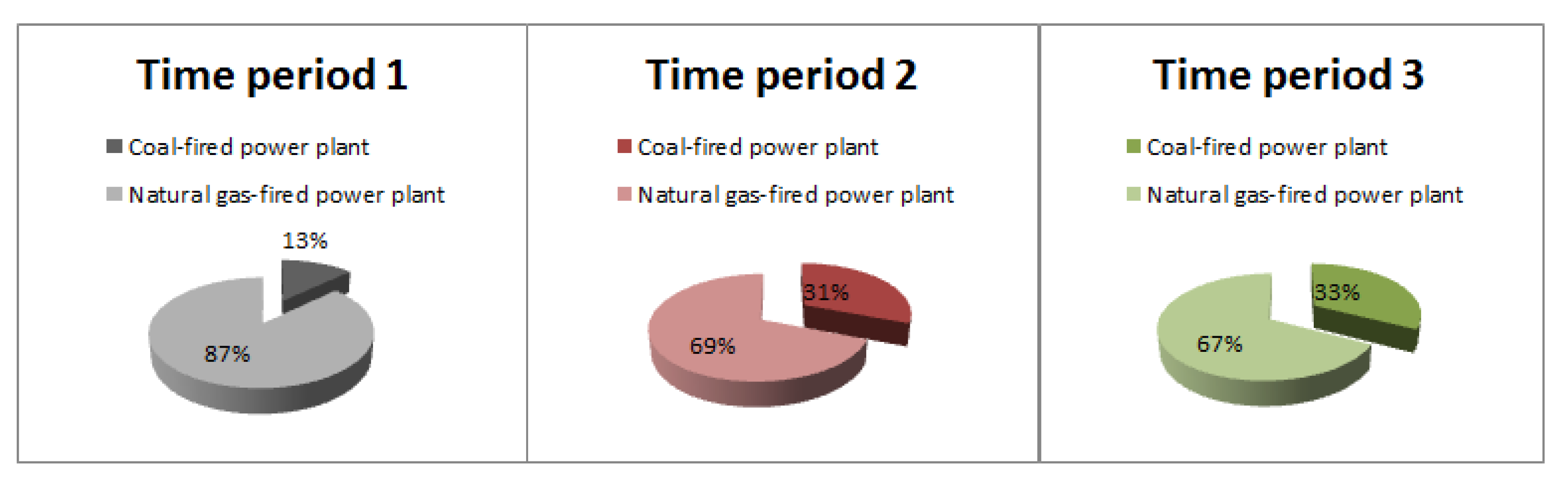
The synthetic computational study is performed or coded in AMPL (A Mathematical Programming Language) and solved using the solver Knitro 5.0, an online free facility offered by the University of Wisconsin, Madison (see [42,43]). The characteristic feature of the implemented EFWS model is 313 variables, 654 inequality constraints, and 402 constants. The total computational time was found to be 0.13 sec. Due to writing restrictions, the EFWS nexus model’s solution results are summarized using the proposed INPA. However, the optimal objectives’ values using different methods are depicted in Table 5 and solution outcomes at various compensation co-efficient are presented in Table 6. The optimal solution results of the EFWS model for the energy, food, and water subsystem network are obtained based on the robust ranking function of the intuitionistic fuzzy parameters. The feasible amount of food production is 23,000, 27,000, and 31,000 tons in all three planning periods, which almost satisfy the socio-economic demands for food efficiently. The optimal and viable distribution of energy-supply from two sources (such as coal and natural gas) are obtained and depicted in Figure 2. From this figure, the allocation of coal is found to be 15%, 28%, and 44% in all the three planning periods, which is significantly increasing. Similarly, natural-gas’ contribution to energy-supply resources is obtained as 85%, 72%, and 56% for all periods, which is reducing. This trend reveals the balancing trade-off between the objectives and constraints where the total economic cost is minimal. The impact of CO emission is comparatively low. For all three planning horizons, the electricity production using different energy-supply is depicted in Figure 3. Due to an increase in electricity demands, the optimal electricity-production policies over the three-time periods are 193.56, 203.87, and 215.61 PJ, respectively, which almost fulfills the socio-economic electricity demands. This is because the extra amount of electricity is needed for food production along with water accumulation, treatment, and supply. The Primary energy-supply source can be considered coal with lesser unit delivery costs over all the planning horizons. Additionally, Figure 3 also indicates each resource (coal and natural gas) to generate electricity. In time period 1, 13% coal and 87% natural-gas are optimally used to produce the required amount of electricity. Similarly, 31% and 33% of coal are consumed in time periods 2 and 3, respectively. The consumption of natural-gas in planning horizons 2 and 3 is obtained as 69% and 67%, which shows a significant contribution towards the electricity-production processes. It is observed because the whole electricity conversion process using natural-gas has very low CO emission rates compared to the coal-fired power plant. Thus, the CO emission abatement can be significantly achieved by using the higher amount of natural-gas resources for GHGs emissions control and environmental protection.
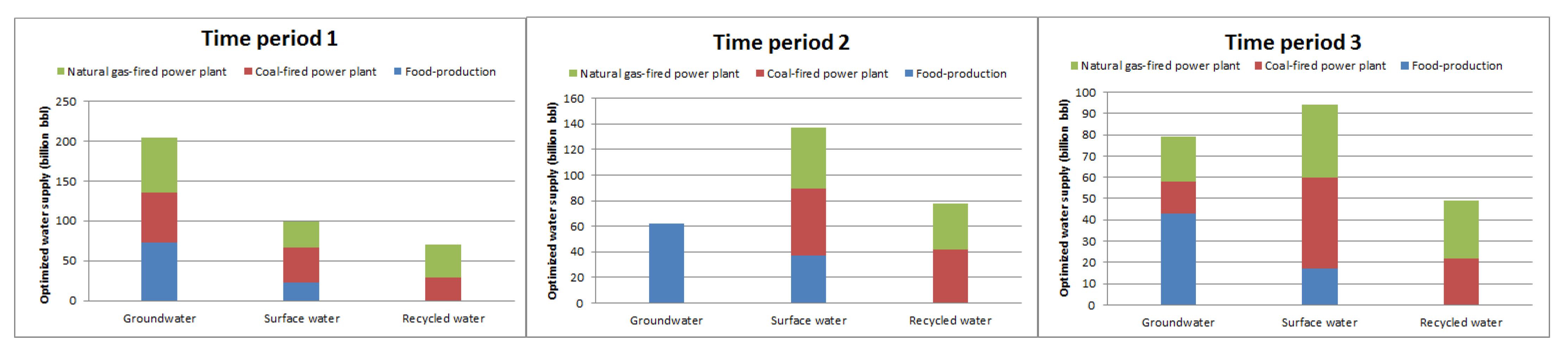
The most exciting finding of the study is that the food production processes require more water resources than electricity production. Since there is no scope for recycled water use for food production (as a health-safety measure), only two kinds of water (groundwater and surface-water) are consumed for food production in all three planning horizons. The optimized allocation of water-resources for food production and electricity conversion is summarized in Figure 4. It can be observed that a higher amount of groundwater is consumed for food production in all three planning horizons; in fact, in time period 2, groundwater is only used for the food production purposes. In planning period 1, the amount of groundwater delivered for the coal and natural-gas-fired plants is slightly lesser than food production. In contrast, in planning periods 2 and 3, the ratio of groundwater for food production is decreased by 73% to 61% and 42%, respectively. It indicates that the significant decrease in groundwater availability will be resulting in water usage flexibility for food production. The production of electricity specifically uses surface-water and recycled water due to its nominal supply costs. In time period 1, only 44, and 31 bbl of groundwater is consumed for coal and natural gas-fired power plants, respectively. The amount of surface water consumed by coal and natural gas-fired power plants is relatively higher than the food production in the remaining two planning periods. This is due to the available amount of groundwater for food production purposes. The preferable option of surface water resources is delivered to coal and natural gas-fired power plant. The recycled water is solely used for electricity conversion purposes in both the coal and natural gas-fired power plant. Hence there are fewer operating and supply costs for surface and recycled water in all the three planning horizons.
4.1.1. Optimal Objectives Values
The optimal socio-economic and environmental objectives are determined using the proposed INPA at different compensation co-efficient and presented in Table 5. At , the total economic costs and CO emissions are 7.19 billion $ and 14.98 million tons, respectively. As the value of increases, both the objective functions reach their worst values, and at , it is obtained as 7.36 billion $ and 15.28 million tons. This pattern is observed because of the preferences between the overall satisfaction level and each objective’s satisfactory individual degree. When the decision-makers are more concerned with the overall satisfaction, then the marginal evaluation of each objective is not significantly achieved, causes worse outcomes, and vice versa. The overall satisfaction level decreases when the compensation coefficient increases. Furthermore, the EFWS nexus model is also solved using (i) Zimmermann [44], (ii) Werners [45], (iii) Selim and Ozkarahan [46], (iv) Torabi and Hassini [47], and results are depicted in Table 6. From the table, it can be concluded that the proposed INPA outperforms others due to the more flexible environment provided by neutrosophic decision-set theory. The existence of indeterminacy or neutral thoughts leads the decision-making process to be more generalized, specifically in calculating each objective’s marginal evaluations. Thus, the proposed EFWS nexus model enables the decision-makers to implement and extract the fruitful findings and information about the optimal allocation, distribution, analyses of the existing policies and strategies of the energy, food, and water resources to achieve the socio-economic and environmental objective at a time.
4.1.2. Sensitivity Analysis
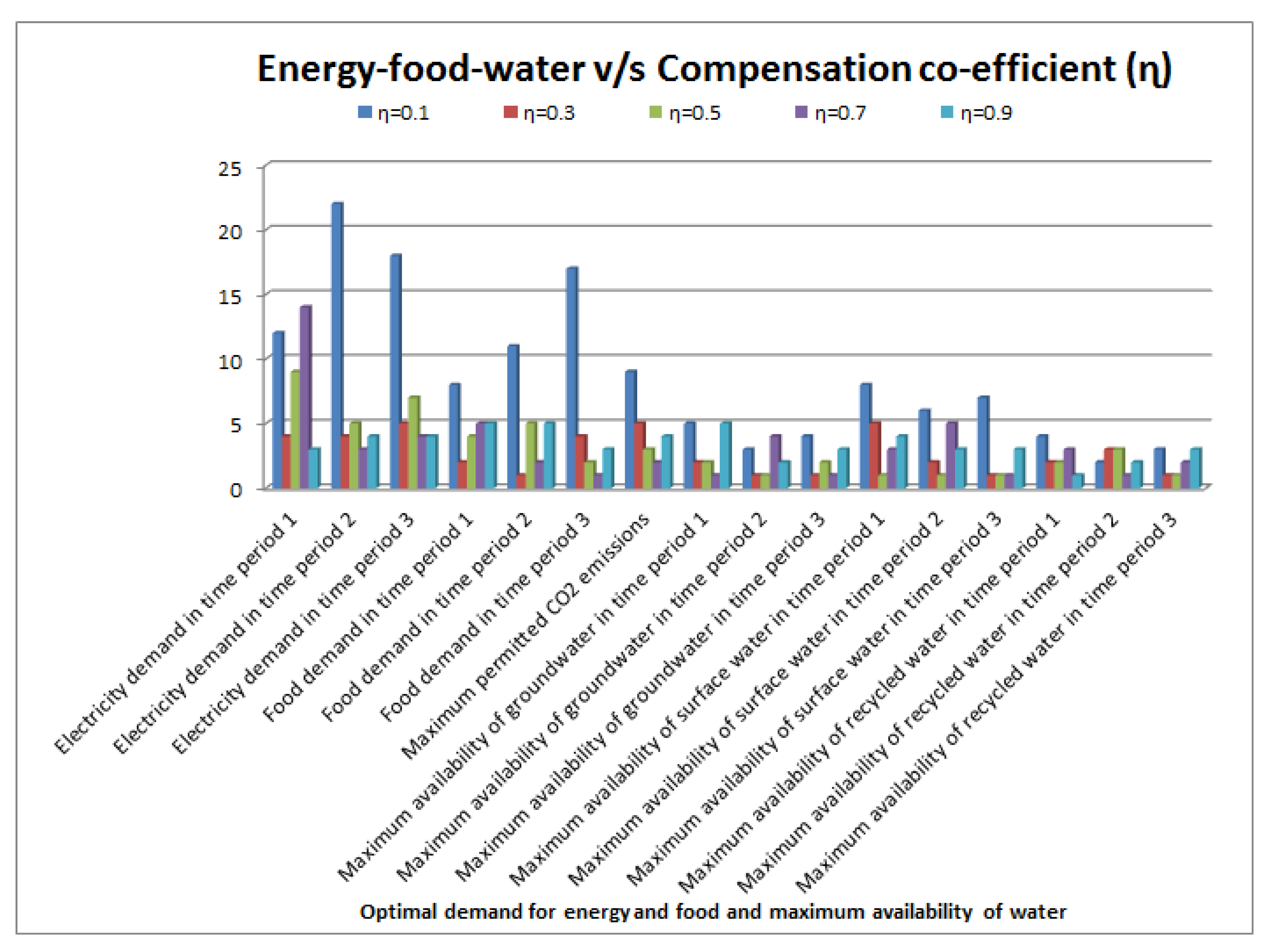
The post-optimality analyses of the implemented EFWS model and the obtained outcomes are performed based on the various aspects. To identify the most sensitive parameters in the EFWS nexus model, different analytical measures have been adopted. The evaluation and analyses of the complexity due to intuitionistic fuzzy parameters over the total economic cost and CO emissions are also examined by tuning the compensation coefficients within the specified ranges and presented in Table 5. The conducted sensitivity analyses reveal that the natural gas supply costs during period 1, coal supply costs, and CO emissions abatement costs in period 3 are the most vulnerable parameters in the EFWS model. Graphical representation of the sensitive parameters is depicted in Figure 5. Moreover, during planning period 1, costs for coal supply is maximum at . Some of the shreds of evidence are also extracted from Figure 6, where each resource’s demands have been significantly achieved in all planning periods at compensation co-efficient . The impact on total economic cost upon splitting the unit costs associated with each sector is depicted in Figure 7. Unit costs for energy supply, electricity, food production, CO emissions abatement, and water supply on the total economic value have been examined. The CO emissions cost has a severe impact on total cost as compared to others. Similarly, the unit costs for energy supply and operating costs of electricity-production are significantly lesser. It means that reducing the expenses of CO emissions abatement will substantially decrease the total economic costs. Practically, the restrictions over resources in the EFWS model may change, such as socio-economic demands for electricity and food, permissible CO emissions, and maximum availability of water (e.g., groundwater, surface, and recycled water) amount.
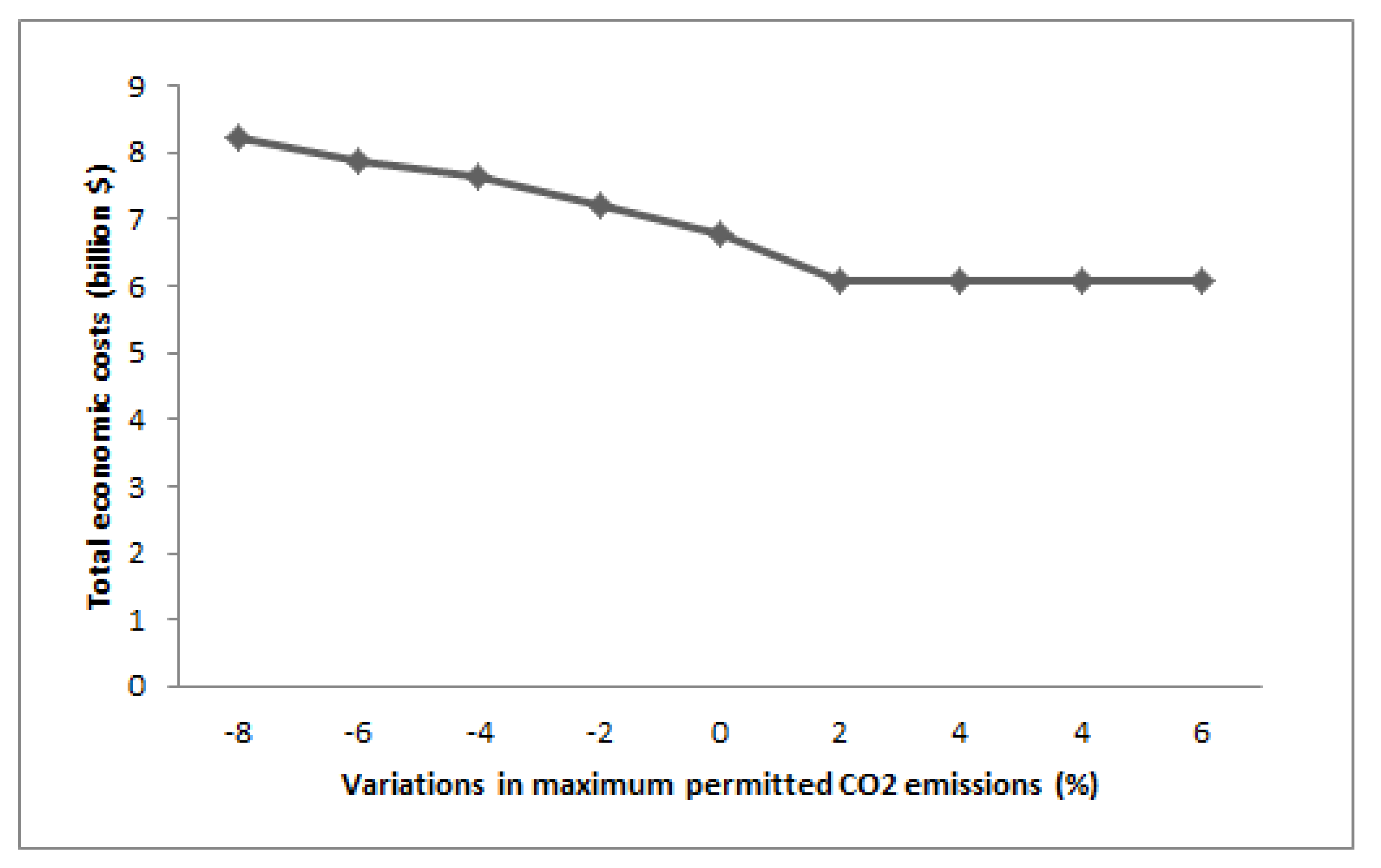
The electricity and food demand has more sensible parameters under uncertainty. It is concluded that as the need for electricity level goes up, the total economic costs also increase rapidly, and consequently, costs of CO emissions abatement are the prime component of the total economic costs. More precisely, weaker restrictions on CO emissions will reduce total economic costs and be shown in Figure 8. Due to the strict constraints imposed over CO emissions abatement, a high amount of electricity will be produced using natural gas-fired power plants; as we know, it has a shallow unit CO emission rate. On the other hand, natural gas-fired power plants for electricity production will maximize total economic costs because of the high delivery and operating costs of the natural gas-fired power plant. To control CO emissions, clean energy strategies with a low CO emissions rate would be adopted even when the associated total economic cost is high. In contrast, the coal-fired power plant may mitigate the total economic cost, but at the same time, CO emissions would be uncontrollable. Hence the balanced trade-offs between socio-economic and environmental objectives are much dependent on the management strategies and fruitful policies. Moreover, based on the sensitivity findings of the EFWS nexus model’s outcomes, when maximum permissible CO emissions approaches at a specified level, the strict restrictions and constraints on the CO emissions protection have no more effect on the total economic costs. It means that the entire system cost will not be further reduced at different values of compensation coefficients. This finding enables the decision-makers or policy-developers to realize the importance of strategic management linked with CO emissions control over socio-economic and environmental protection.
Furthermore, it is observed that the demand for food and the maximum amount of water availability are comparatively less than the energy demand and the maximum permissible CO emissions rate. The intricacies for energy-supply, electricity-production, and water delivery will also fluctuate in all three planning horizons. The maximum amount of available groundwater, surface, and recycled water may drastically change based on climatic and geographical conditions. For a 13% decrease in the total available water (groundwater, surface, and recycled water), the total economic cost would be trivially increased by $3.62 billion. Variation in the available water quantity leads to the relative change in the optimal water distribution of all sorts of water resources among the candidate location in the EFWS nexus model. Depending on the sufficient water resources availability, electricity conversion and food production may use enough water with lesser delivery costs, resulting in reduced total economic costs. Therefore, the optimal allocation and wholesome usage planning of water resources are the most typical and challenging tasks for the inter-connected EFWS nexus management and, consequently, for water resources conservation.
4.1.3. Discussions and Practical Implications
The prime motive behind developing the proposed EFWS nexus model is to highlight and explore the basic resources management system by identifying and determining the optimal allocation of these resources in the most critical aspects of socio-economic crisis and environmental impacts. The proposed EFWS model is good enough to address the complex configuration of interconnected energy, food, and water network from a realistic point of view. Tradeoffs between socio-economic and environmental objectives, available resources constraints, and their optimal distribution are efficiently quantified over the planning periods. Since the proposed EFWS nexus model is designed for multi-period scenarios, EFWS has a high tendency to grab the temporary characteristic features of the energy-food-water management systems and capabilities to create the cost-effective policies and opportunities for optimizing EFWS production/Supply and reduction linked with the environmental impacts (i.e., GHG emissions). This study considered the two sorts of energy-supply sources (coal and natural gas); however, the proposed EFWS nexus model can be extended by introducing other energy (e.g., wind, solar, petroleum). The additional variables and parameters can be incorporated without changing the proposed EFWS nexus model’s actual structure. Although the EFWS model exhibits a high-level of complexity in both structural and computational aspects, EFWS will be more justified and applicable for large-scale real-life applications at state and national levels. There is ample opportunity for decision-makers to develop and build their problem-oriented applications based on importance and necessities.
Uncertainty is tackled using intuitionistic fuzzy set theory, which guarantees less violation of risks due to vagueness and hesitations during decision-making processes. Different compensation co-efficient also provides flexibility while assigning the priorities to each objective and corresponding to their marginal evaluation (acceptance degrees). We have performed this study to highlight and explore a decision analysis technique to identify and address the EFWS nexus management under uncertainty at states and national levels. Because of this, we have undertaken only the most indispensable EFWS components such as energy and water supplies, electricity conversion, food production, and CO emissions abatement at the utmost priority. The same electricity and food demands are not easily predictable under the vague uncertainty but using the intuitionistic fuzzy set concept, and it can be accurately estimated based on the robust ranking function method and gives a better representation than the stochastic and fuzzy models in EFWS nexus management systems. The proposed EFWS is accountable for the EFWS nexus model’s temporary scenario and cannot discuss the spatial dimensions. The EFWS nexus model’s spatial configuration may realize some effects on the obtained decision outcomes policies but are untouched in the EFWS model, which is consistent in matching targets of the proposed EFWS nexus model at states and national levels.
The propounded EFWS nexus model has some limitations. Generally, the EFWS management network’s modeling structure can be very complex, and the EFWS nexus model is not exhibiting a wholesome framework for all feasible elements and strategies linked with social, cultural, territorial issues. Moreover, the inequalities and restrictions due to lack of available energy, food, and water resources for security purposes also makes it complicated under the critical circumstances. A few inter-connected relationships between society and environment such as food production, energy and water supply, and CO emission control is considered in the proposed EFWS nexus model. Various inter-dependence issues such as energy, food and water resources ejaculations and emissions with their side-effects on ecological system are left untouched. The required amount of energy for water and food production susbsystems are derived with the aid of unit energy requirement for water collection, treatment and supply, and food production, respectively. In contrast, required amount of water for electricity and food production are approximated with the help of unit demand for water per unit of electricity and food production, respectively, instead of straight-forward measuring methods. Estimations for societal demands of electricity, food and water have been done in all three planning horizons.
The future research scope is also opened by modifying and extending the proposed EFWS nexus model. Different forms of uncertainties in parameters’ values can be discussed based on essence of need. For vague information, fuzzy techniques can be applied whereas for historical data-set, the stochastic techniques can be adopted to obtain the deterministic version. Assessments of accuracy and robustness in the decision-support system against uncertainties are also topic of deep interest for the proposed EFWS nexus model. Environmental factors such as climate change, weather conditions etc. are not effectively discussed into the proposed EFWS nexus model; fluctuation in these may cause significant changes in energy, food and water resources, and correspondingly the obtained EFWS management policies. The implementation of climatic factors will definitely assists the optimal EFWS nexus management system for climate adaptation and resilience planning according to the fluctuation in environmental impacts. Closer to reality, the need-oriented and specific information can be considered based on the local hydrological, glaciological, oceanological, climatological and geographical conditions. Simultaneously, the complexity among EFWS nexus model can also be tackled with its inter-connected components. The proposed EFWS nexus model is implemented and analyzed on the hypothetical and secondary data-set which is much closer and sufficient to illustrate the real-life applications; however, we hope to execute the proposed modeling and optimization approach real-world case studies in the future.
5. Conclusions
A dynamic and versatile EFW security nexus management model is developed under the intuitionistic fuzzy uncertainty. The integrated component of the EFWS model provides a robust decision analyses support system for an optimal allocation of energy-food-water resources. The proposed EFWS model is formulated as a multi-period, multi-dimensional linear programming problem. Different components of the EFWS nexus management system include the strategies and policies for energy and water supplies, electricity, and food production, energy-food-water demand, and emission protection. The socio-economic and environmental objectives are depicted for the optimal allocation of the resources in different planning horizons. The EFWS model has enough potential to identify and address the inter-dependence among energy-food-water subsystems. The effects on optimal decision support system as well while dealing with security nexus management. The proposed EFWS model is implemented on a synthetic nexus planning problem, which is more reliable and consistent in matching the real-life management aspects. The optimal economic and environmental objectives are determined using the discussed approaches and the proposed INPA. Strategies and policies for the optimal allocation of the available and limited energy supplies, electricity and food production, and water resources are addressed for fulfilling the expected demand of the society.
Following are the significant findings/contributions to this study.
- The proposed EFWS model may assist the decision-makers and policy-developers in arriving at the optimal decision without violating the risk uncertainty due to hesitation. Moreover, the policy-makers may avail the sequential and most promising alternatives for the robust EFWS management network by adjusting the socio-economic demands of electricity, food, and water resources along with the ecological impacts restrictions.
- The established trade-offs among the socio-economic and environmental objectives, resource restrictions, and CO emission control would be feasible in applying the practical EFWS nexus management system.
- The analyzed effects of parameters’ values reveal that when decision-makers are more concerned about uncertainty, it will lead to the worst objectives (both economic and environmental) and vice versa.
- It is concluded that high socio-economic demands for electricity, food, and water resources will result in higher financial cost and simultaneously high CO emissions. The increment in the amount of maximum available water resources and permissible CO emission would reduce the total economic costs.
- The proposed EFWS nexus model is reliable in tackling the uncertainty and is computationally efficient in implementing large-scale energy-food-water nexus management systems.
- The need for electricity and food will also enhance the CO emissions in both the processes. The outcomes support the modeling approach and emphasize the essence of using and analyzing the proposed EFWS nexus management system.
- It can be useful for decision-makers and policy-developers to identify, quantify, and establish the trade-offs among typical inter-connections between energy, food, and water subsystems and to arrive at a decision for an integrated energy-food-water management system.
5.1. Treating Intuitionistic Fuzzy Parameters
For treating intuitionistic fuzzy parameters, we discussed important definitions of the intuitionistic fuzzy set (IFS).
Definition 3.
In [48] (IFS) they assume that there be a universal set X. Then, an intuitionistic fuzzy set in X is defined by the ordered triplets as follows:
where denotes the membership function and denotes the non-membership function of the element into the set , respectively, with the conditions . The value of , is called the degree of uncertainty of the element to the IFS . If , an IFS becomes fuzzy set and takes the form .
Definition 4.
In [5] a triangular intuitionistic fuzzy number (TrIFN) is represented by where such that ; and its membership function and non-membership function is of the form
Definition 5.
In [5], they consider that a TrIFN is given by where such that . Then the parametric form of are and . Furthermore, and are the parametric form of TrIFN corresponding to membership and non-membership functions such that , and , respectively. A TrIFN is said to be positive TrIFN if and hence are all positive numbers.
Definition 6.
(Expected interval and expected value of TrIFNs) The concept of expected interval and expected value was defined by Heilpern [49]. Thus, we re-defined it for TrIFNs. Suppose that be a TrIFN and and depict the expected intervals for membership and non-membership functions respectively. Thus, these can be defined as follows:
Moreover, consider that and represent the expected values corresponding to membership and non-membership functions respectively. These can be depicted as follows:
The expected value of a TrIFN is given as follows:
5.2. Solution Methodology
This section describes the various solution approaches for solving the multiobjective programming problems (MOPPs). Usually, it is very difficult to determine the single solution set which satisfies each objective functions potentially, however, a compromise solution can be determined using the multiobjective optimization techniques. Let us consider the general form of MOPPs (24):
where is the set of decision variables. is the objective function and is the real-valued functions in . The vector is the right hand-side constant, repectively.
To solve the MOPPs (24), first each objective function is solved under the set of given constraints. The maximum and minimum values of each objective function are depicted as follows (25):
Afterward the marginal evaluations of each objective function is obtained, known as membership functions . Thus, the membership functions for objective function can be defined as follows (26):
Here, we briefly discuss the four different multiobjective optimization techniques: (i) Zimmermann [44], (ii) Werners [45], (iii) Selim and Ozkarahan [46] and (iv) Torabi and Hassini [47], respectively. Apart from this, we have proposed a novel solution method called iterative neutrosophic programming approach (INPA) and elaborately discussed in Section 3.2.1.
5.2.1. Zimmermann’s Method
5.2.2. Werners’ Method
According to Werners [45], the MOPPs (24) can be transformed into the equivalent single objective programming problem as follows (28):
where has the same meaning as in Zimmermann [44] approach and is the individual satisfaction level of each objectives. Further is the compensation co-efficient among the objective functions. Thus, the achievement function is defined as the convex combination of the overall satisfactory degree of all objectives and the sum of individual satisfaction level of each objective functions, and can be attained by maximizing it.
5.2.3. Selim and Ozkarahan’s Approach
The method suggested by Selim and Ozkarahan [46] have taken the advantage of weightage scheme assigned to each objective functions according to the decision-makers’ preferences. An opportunity to put the relative importance among the objective function is depicted by introducing the crisp weight and transformed the MOPPs (24) into the equivalent single objective programming problem as follows (29):
where all the notations have same meaning as in Werners [45].
5.2.4. Torabi and Hassini’s Optimization Technique
According to Torabi and Hassini [47] optimization technique, the overall satisfaction level is defined as the convex combination of minimum satisfaction degree of each objectives and the weighted sum of each membership functions of all objective function simultaneously. Thus, the equivalent single objective programming problem for the MOPPs (24) can be summarized as follows (30):
Author Contributions
Conceptualization, F.A.; Methodology, F.A.; Formal analysis, M.Z.; Writing—original draft preparation, F.A.; Writing—review and editing, F.A.; Project administration, A.Y.A.; Funding acquisition, S.A.; Software, F.A., A.Y.A.; Validation, S.A., F.A.; Investigation, S.A.; Data curation, A.Y.A. All authors have read and agreed to the published version of the manuscript.
Funding
The authors extend their appreciation to the Deputyship for Research & Innovation, “Ministry of Education” in Saudi Arabia for funding this research work through the project number IFKSURG-1438-089.
Data Availability Statement
Data is available within the manuscript.
Acknowledgments
The authors are very overwhelmed by and thankful to anonymous reviewers and editors for their insightful comments to make the manuscript more clear and readable. The first author is very thankful to Indian Statistical Institute, Kolkata for providing the various research facilities during revision of the manuscript.
Conflicts of Interest
No conflict of interest is reported by authors.
References
- US Energy Information Administration. How much Carbon Dioxide Is Produced Per Kilowatthour When Generating Electricity with Fossil Fuels; US Energy Information Administration: Washington, DC, USA, 2015.
- Diehl, T.H.; Harris, M.A. Withdrawal and Consumption of Water by Thermoelectric Power Plants in the United States, 2010; USGS: Reston, VA, USA, 2014.
- FAO. The Water-Energy-Food Nexus: A New Approach in Support of Food Security and Sustainable Agriculture; FAO: Rome, Italy, 2014. [Google Scholar]
- Bazilian, M.; Rogner, H.; Howells, M.; Hermann, S.; Arent, D.; Gielen, D.; Steduto, P.; Mueller, A.; Komor, P.; Tol, R.S.; et al. Considering the energy, water and food nexus: Towards an integrated modelling approach. Energy Policy 2011, 39, 7896–7906. [Google Scholar] [CrossRef]
- Ahmad, F.; Adhami, A.Y.; Smarandache, F. Neutrosophic Optimization Model and Computational Algorithm for Optimal Shale Gas Water Management under Uncertainty. Symmetry 2019, 11, 544. [Google Scholar] [CrossRef] [Green Version]
- Bieber, N.; Ker, J.H.; Wang, X.; Triantafyllidis, C.; van Dam, K.H.; Koppelaar, R.H.; Shah, N. Sustainable planning of the energy-water-food nexus using decision making tools. Energy Policy 2018, 113, 584–607. [Google Scholar] [CrossRef]
- Uen, T.S.; Chang, F.J.; Zhou, Y.; Tsai, W.P. Exploring synergistic benefits of Water-Food-Energy Nexus through multi-objective reservoir optimization schemes. Sci. Total Environ. 2018, 633, 341–351. [Google Scholar] [CrossRef] [PubMed]
- Tsolas, S.D.; Karim, M.N.; Hasan, M.F. Optimization of water-energy nexus: A network representation-based graphical approach. Appl. Energy 2018, 224, 230–250. [Google Scholar] [CrossRef]
- Namany, S.; Al-Ansari, T.; Govindan, R. Sustainable energy, water and food nexus systems: A focused review of decision-making tools for efficient resource management and governance. J. Clean. Prod. 2019, 225, 610–626. [Google Scholar] [CrossRef]
- Gao, J.; Xu, X.; Cao, G.; Ermoliev, Y.M.; Ermolieva, T.Y.; Rovenskaya, E.A. Optimizing regional food and energy production under limited water availability through integrated modeling. Sustainability 2018, 10, 1689. [Google Scholar] [CrossRef] [Green Version]
- Zhang, T.; Tan, Q.; Yu, X.; Zhang, S. Synergy assessment and optimization for water-energy-food nexus: Modeling and application. Renew. Sustain. Energy Rev. 2020, 134, 110059. [Google Scholar] [CrossRef]
- Li, G.; Wang, Y.; Li, Y. Synergies within the Water-Energy-Food Nexus to Support the Integrated Urban Resources Governance. Water 2019, 11, 2365. [Google Scholar] [CrossRef] [Green Version]
- Hamidov, A.; Helming, K. Sustainability Considerations in Water–Energy–Food Nexus Research in Irrigated Agriculture. Sustainability 2020, 12, 6274. [Google Scholar] [CrossRef]
- Saif, Y.; Almansoori, A.; Bilici, I.; Elkamel, A. Sustainable management and design of the energy-water-food nexus using a mathematical programming approach. Can. J. Chem. Eng. 2020. [Google Scholar] [CrossRef]
- Ji, L.; Zheng, Z.; Wu, T.; Xie, Y.; Liu, Z.; Huang, G.; Niu, D. Synergetic optimization management of crop-biomass coproduction with food-energy-water nexus under uncertainties. J. Clean. Prod. 2020, 258, 120645. [Google Scholar] [CrossRef]
- Okola, I.; Omullo, E.O.; Ochieng, D.O.; Ouma, G. A Multiobjective Optimisation Approach for Sustainable Resource Consumption and Production in Food-Energy-Water Nexus. In Proceedings of the 2019 IEEE AFRICON, Accra, Ghana, 25–27 September 2019; pp. 1–5. [Google Scholar]
- Li, M.; Fu, Q.; Singh, V.P.; Ji, Y.; Liu, D.; Zhang, C.; Li, T. An optimal modelling approach for managing agricultural water-energy-food nexus under uncertainty. Sci. Total Environ. 2019, 651, 1416–1434. [Google Scholar] [CrossRef] [PubMed]
- Li, M.; Fu, Q.; Singh, V.P.; Liu, D.; Li, T. Stochastic multi-objective modeling for optimization of water-food-energy nexus of irrigated agriculture. Adv. Water Resour. 2019, 127, 209–224. [Google Scholar] [CrossRef]
- Li, M.; Fu, Q.; Singh, V.P.; Liu, D.; Li, J. Optimization of sustainable bioenergy production considering energy-food-water-land nexus and livestock manure under uncertainty. Agric. Syst. 2020, 184, 102900. [Google Scholar] [CrossRef]
- Yu, L.; Xiao, Y.; Jiang, S.; Li, Y.; Fan, Y.; Huang, G.; Lv, J.; Zuo, Q.; Wang, F. A copula-based fuzzy interval-random programming approach for planning water-energy nexus system under uncertainty. Energy 2020, 196, 117063. [Google Scholar] [CrossRef]
- Elsayed, H.; Djordjević, S.; Savić, D.A.; Tsoukalas, I.; Makropoulos, C. The Nile Water-Food-Energy Nexus under Uncertainty: Impacts of the Grand Ethiopian Renaissance Dam. J. Water Resour. Plan. Manag. 2020, 146, 04020085. [Google Scholar] [CrossRef]
- Tan, Q.; Zhang, T. Robust fractional programming approach for improving agricultural water-use efficiency under uncertainty. J. Hydrol. 2018, 564, 1110–1119. [Google Scholar] [CrossRef]
- Hurford, A. Accounting for Water-, Energy-and Food-Security Impacts in Developing Country Water Infrastructure Decision-Making under Uncertainty. Ph.D. Thesis, University College London, London, UK, 2016. [Google Scholar]
- Govindan, R.; Al-Ansari, T. Computational decision framework for enhancing resilience of the energy, water and food nexus in risky environments. Renew. Sustain. Energy Rev. 2019, 112, 653–668. [Google Scholar] [CrossRef]
- Ji, L.; Zhang, B.; Huang, G.; Lu, Y. Multi-stage stochastic fuzzy random programming for food-water-energy nexus management under uncertainties. Resour. Conserv. Recycl. 2020, 155, 104665. [Google Scholar] [CrossRef]
- Yu, L.; Xiao, Y.; Zeng, X.; Li, Y.; Fan, Y. Planning water-energy-food nexus system management under multi-level and uncertainty. J. Clean. Prod. 2020, 251, 119658. [Google Scholar] [CrossRef]
- Hang, M.Y.L.P.; Martinez-Hernandez, E.; Leach, M.; Yang, A. Designing integrated local production systems: A study on the food-energy-water nexus. J. Clean. Prod. 2016, 135, 1065–1084. [Google Scholar] [CrossRef]
- Martinez-Hernandez, E.; Leach, M.; Yang, A. Understanding water-energy-food and ecosystem interactions using the nexus simulation tool NexSym. Appl. Energy 2017, 206, 1009–1021. [Google Scholar] [CrossRef]
- Smarandache, F. A Unifying Field in Logics: Neutrosophic Logic. In Philosophy; American Research Press: Rehoboth, DE, USA, 1999; pp. 1–141. [Google Scholar]
- Ahmad, F.; Adhami, A.Y. Neutrosophic programming approach to multiobjective nonlinear transportation problem with fuzzy parameters. Int. J. Manag. Sci. Eng. Manag. 2019, 14, 218–229. [Google Scholar] [CrossRef]
- Ahmad, F.; Adhami, A.Y.; Smarandache, F. 15—Modified neutrosophic fuzzy optimization model for optimal closed-loop supply chain management under uncertainty. In Optimization Theory Based on Neutrosophic and Plithogenic Sets; Smarandache, F., Abdel-Basset, M., Eds.; Academic Press: New York, NY, USA, 2020; pp. 343–403. [Google Scholar]
- Adhami, A.Y.; Ahmad, F. Interactive Pythagorean-hesitant fuzzy computational algorithm for multiobjective transportation problem under uncertainty. Int. J. Manag. Sci. Eng. Manag. 2020, 15, 288–297. [Google Scholar] [CrossRef]
- Ahmad, F.; Adhami, A.Y. Total cost measures with probabilistic cost function under varying supply and demand in transportation problem. Opsearch 2019, 56, 583–602. [Google Scholar] [CrossRef]
- Ahmad, F.; Adhami, A.Y.; Smarandache, F. Single Valued Neutrosophic Hesitant Fuzzy Computational Algorithm for Multiobjective Nonlinear Optimization Problem. Neutrosophic Sets Syst. 2018, 22, 76–86. [Google Scholar] [CrossRef]
- Bellman, R.E.; Zadeh, L.A. Decision-Making in a Fuzzy Environment. Manag. Sci. 1970, 17, 141–164. [Google Scholar] [CrossRef]
- Canning, P.N. Fuel for Food: Energy Use in the US Food System; Technical Report; United States Department of Agriculture, Economic Research Service: Washington, DC, USA, 2010.
- Hellegers, P.; Zilberman, D.; Steduto, P.; McCornick, P. Interactions between water, energy, food and environment: Evolving perspectives and policy issues. Water Policy 2008, 10, 1–10. [Google Scholar] [CrossRef]
- Change, O.C. Intergovernmental Panel on Climate Change; WMO: Geneva, Switzerland; UNEP: Athens, Greece, 2007. [Google Scholar]
- Montagnini, F.; Ibrahim, M.; Murgueitio, E. Silvopastoral systems and climate change mitigation in Latin America. Bois. ForÊTs Des. Trop. 2013, 316, 3–16. [Google Scholar] [CrossRef]
- Zhang, X.; Huang, G. Optimization of environmental management strategies through a dynamic stochastic possibilistic multiobjective program. J. Hazard. Mater. 2013, 246, 257–266. [Google Scholar] [CrossRef] [PubMed]
- Li, G.; Huang, G.; Lin, Q.; Zhang, X.; Tan, Q.; Chen, Y. Development of a GHG-mitigation oriented inexact dynamic model for regional energy system management. Energy 2011, 36, 3388–3398. [Google Scholar] [CrossRef]
- Dolan, E. The Neos Server 4.0 Administrative Guide; Technical Report; Memorandum ANL/MCS-TM-250; Mathematics and Computer Science Division, Argonne National Laboratory: Argonne, IL, USA, 2001.
- Drud, A.S. CONOPT—A large-scale GRG code. ORSA J. Comput. 1994, 6, 207–216. [Google Scholar] [CrossRef]
- Zimmermann, H.J. Fuzzy programming and linear programming with several objective functions. Fuzzy Sets Syst. 1978, 1, 45–55. [Google Scholar] [CrossRef]
- Werners, B.M. Aggregation models in mathematical programming. In Mathematical Models for Decision Support; Springer: New York, NY, USA, 1988; pp. 295–305. [Google Scholar]
- Selim, H.; Ozkarahan, I. A supply chain distribution network design model: An interactive fuzzy goal programming-based solution approach. Int. J. Adv. Manuf. Technol. 2008, 36, 401–418. [Google Scholar] [CrossRef]
- Torabi, S.A.; Hassini, E. An interactive possibilistic programming approach for multiple objective supply chain master planning. Fuzzy Sets Syst. 2008, 159, 193–214. [Google Scholar] [CrossRef]
- Atanassov, K.T. Intuitionistic fuzzy sets. Fuzzy Sets Syst. 1986, 20, 87–96. [Google Scholar] [CrossRef]
- Heilpern, S. The expected value of a fuzzy number. Fuzzy Sets Syst. 1992, 47, 81–86. [Google Scholar] [CrossRef]
Figure 1.
Inter-dependence relationships of Energy-Food-Water security nexus management system.
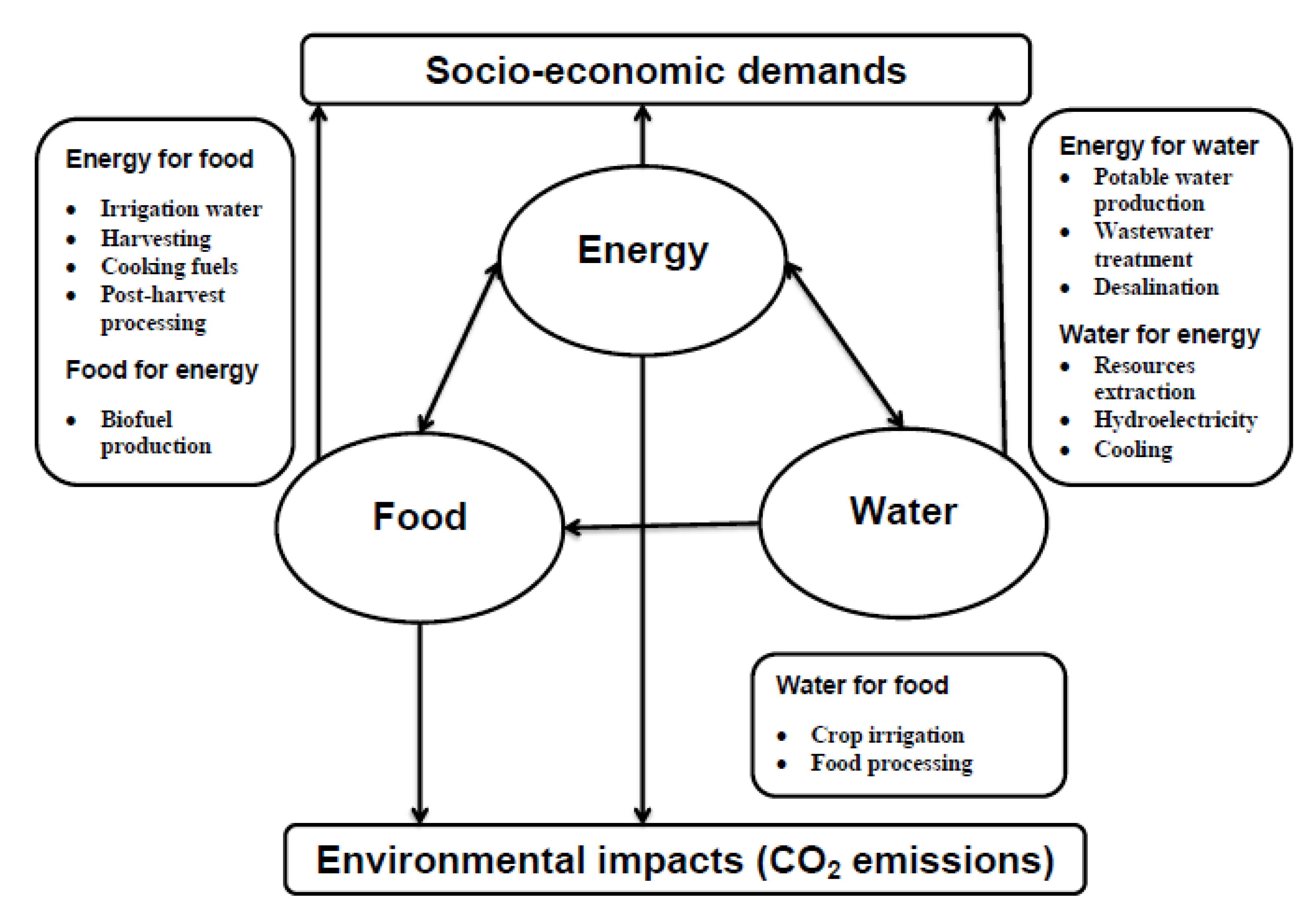
Figure 2.
Optimal energy-supply in proposed EFWS model (PJ).
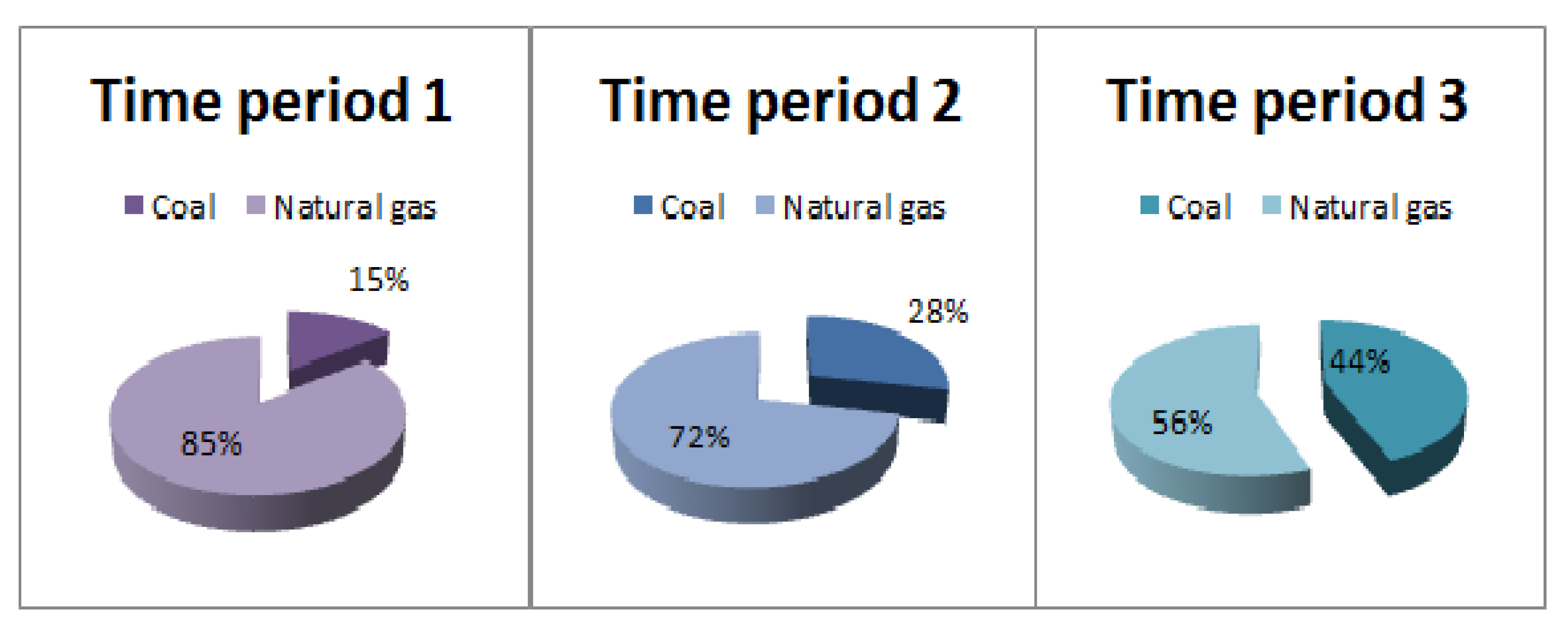
Figure 3.
Optimal electricity-production in proposed EFWS model (PJ).

Figure 4.
Optimal amount of water supply for food and electricity production in proposed EFWS model.
Figure 4.
Optimal amount of water supply for food and electricity production in proposed EFWS model.

Figure 5.
Effects of variations in unit costs due to changes in the compensation co-efficient in proposed EFWS model.
Figure 5.
Effects of variations in unit costs due to changes in the compensation co-efficient in proposed EFWS model.
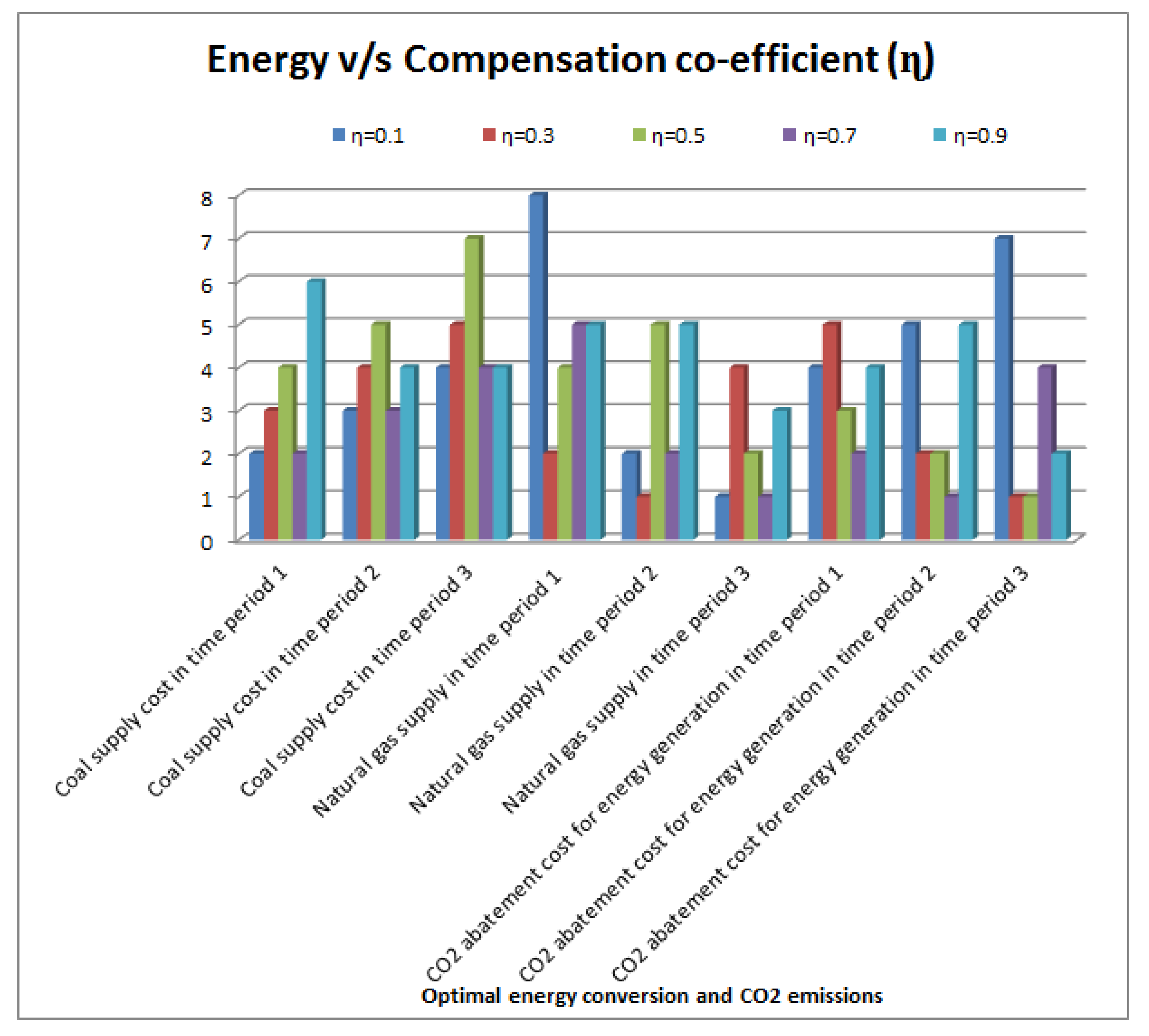
Figure 6.
Effects of variations in resource constraints due to changes in the compensation co-efficient in proposed EFWS model.
Figure 6.
Effects of variations in resource constraints due to changes in the compensation co-efficient in proposed EFWS model.

Figure 7.
Effects of variations in unit costs due to the total economic cost.
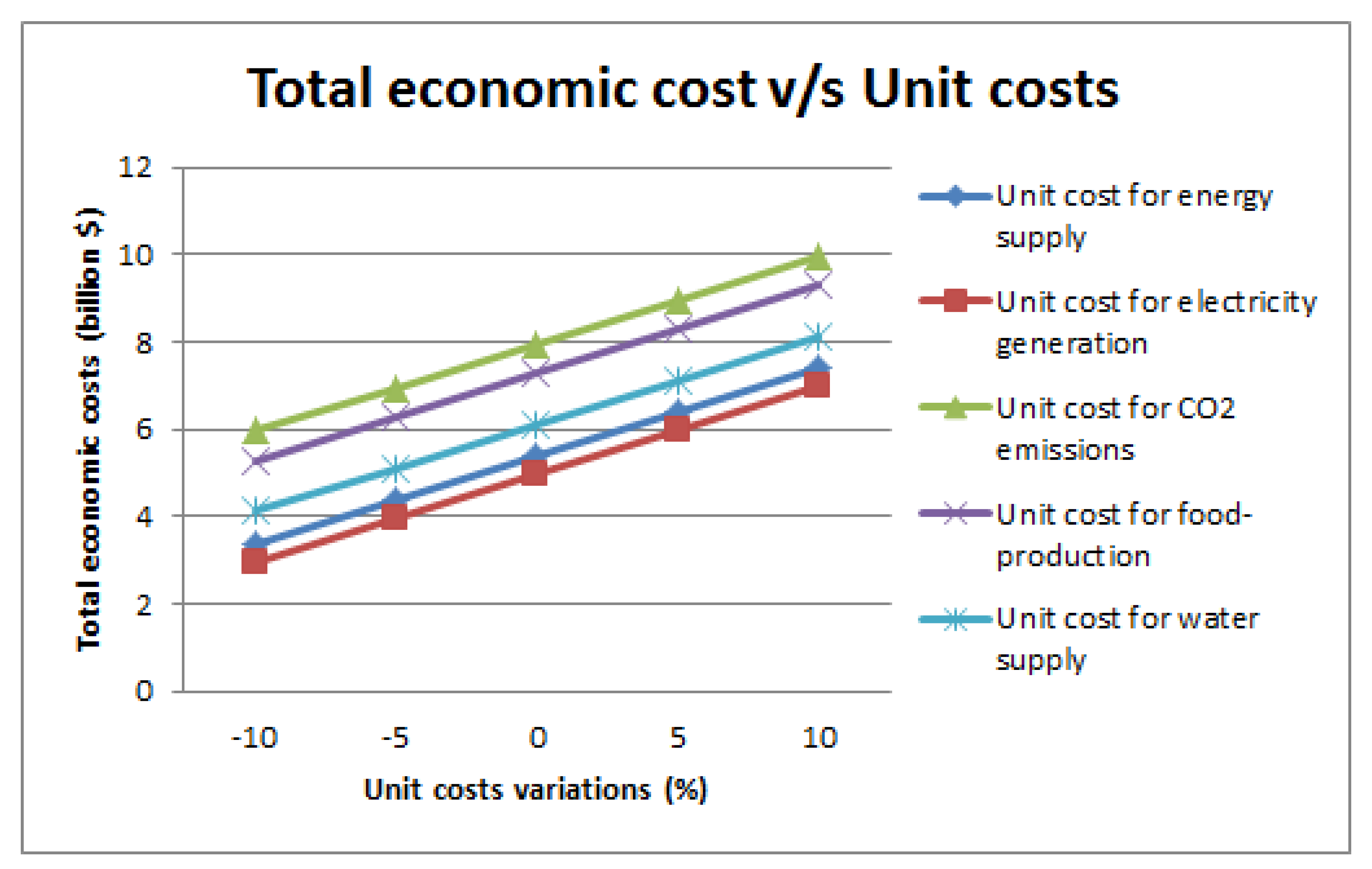
Figure 8.
Effects of variations in emissions due to the total economic cost.

Table 1.
Notions and descriptions.
| Indices | Descriptions |
|---|---|
| e | Associated with the energy-production |
| f | Associated with the food production |
| Denotes the types of available energy supply and power conversion plant | |
| Represents the effective planning time periods such as a time horizon for energy, food and water security management | |
| w | Associated with the water-resources use |
| Decision variables | |
| Amount of available energy supply j in time period t (PJ) | |
| Amount of electricity conversion by a power plant o using energy supply j in time period t (PJ) | |
| Quantity of groundwater consumed in food production processes in time period t (bbl) | |
| Quantity of surface water consumed in food production processes in time period t (bbl) | |
| Groundwater quantity delivered to power-conversion plant j in time period t (bbl) | |
| Surface water quantity delivered to power-conversion plant j in time period t (bbl) | |
| Amount of recycled water sent to power-conversion plant j in time period t (bbl) | |
| Total quantity of food production in time period t (ton) | |
| Parameters | |
| Average cost associated with energy supply j in time period t (million $/PJ) | |
| Fixed cost associated with power conversion plant j (million $) | |
| Average operational cost incurred over electricity production by power conversion plant j in time period t (million $/PJ) | |
| Total cost related to groundwater supply for food production in time horizon t ($/bbl) | |
| Total cost related to groundwater supply for power conversion plant j in time horizon t ($/bbl) | |
| Total cost related to surface water supply for food production in time horizon t ($/bbl) | |
| Total cost related to surface water supply for power conversion plant j in time horizon t ($/bbl) | |
| Total cost related to recycled water supply for power conversion plant j in time horizon t ($/bbl) | |
| Unit cost associated with food production in time period t (million $/ton) | |
| Total cost of CO emission abatement for electricity production in time period t ($/kg) | |
| Units of CO emission per unit of electricity production by power conversion plant j in time period t (million kg/PJ) | |
| Total cost of CO emission abatement for food production in time period t ($/ton) | |
| Units of CO emission per unit of food production in time period t (million kg/ton) | |
| Unit energy carrier per unit of electricity production for transformation technique j in time period t (PJ/PJ) | |
| Total available energy supply j in time period t (PJ) | |
| Maximum unit of electricity available for food production in time period t (PJ) | |
| Maximum unit of electricity available for water collection, treatment and supply in time period t (PJ) | |
| Demand of unit energy for food production in time period t (PJ/ton) | |
| Demand of unit energy for water collection, treatment and supply in time period t (PJ) | |
| Socio-economic demand for energy (or electricity) in time period t (PJ) | |
| Socio-economic demand for food in time period t (ton) | |
| Units of water consumption per unit of food production in time period t (bbl/ton) | |
| Maximum quantity of available groundwater safe yield in time period t (bbl) | |
| Maximum quantity of available surface water in time period t (bbl) | |
| Maximum quantity of available recycled water in time period t (bbl) | |
| Maximum permissable CO emission during planning periods (million ton) | |
| Loss factor of water supply to the food sub-system | |
| Unit water demand per unit of electricity production by power conversion plant j (bbl/GWh) | |
| Loss factor of water supply to the power conversion plant j | |
| Average efficiency factor for CO emission abatement by power conversion plant j in time period t |
Table 2.
Different intuitionistic fuzzy cost parameters related to associated services.
| Time Period (05 Years Each) | |||
|---|---|---|---|
| Average operational costs | |||
| Coal supplies (million $/PJ) | (3.0,3.2,3.4;2.8,3.2,3.6) | (3.4,3.6,3.8;3.2,3.6,4.0) | (3.8,4.0,4.2;3.6,4.2,4.4) |
| Natural gas supplies (million $/PJ) | (5.2,5.6,6.0;4.8,5.6,6.2) | (6.0,6.3,6.6;5.8,6.3,6.8) | (6.6,6.7,6.8;6.4,6.7,6.9) |
| Electricity production in | (6.0,6.5,7.0;5.8,6.5,7.2) | (6.6,6.9,7.2;6.4,6.9,7.4) | (7.1,7.4,7.7;6.8,7.4,7.9) |
| coal-fired plant (million $/PJ) | |||
| Electricity production in | (2.8,2.9,3.0;2.4,2.9,3.3) | (3.5,3.7,3.9;3.2,3.74.2) | (4.2,4.4,4.6;3.8,4.4,4.8) |
| natural gas-fired plant (million $/PJ) | |||
| Unit food production cost ($/ton) | (3.2,3.4,3.6;2.8,3.4,4.0) | (3.5,3.9,4.3;3.2,3.9,4.2) | (4.1,4.2,4.3;3.8,4.2,4.4) |
| Costs of COemissions abatement | |||
| For electricity production ($/million kg) | (14.2,14.4,14.6;14.0,14.4,14.8) | (12.1,12.3,12.5;12.0,12.3,12.6) | (13.1,13.3,13.5;13.0,13.3,13.6) |
| For food production ($/ton) | (12.2,12.5,12.8;12.1,12.5,12.9) | (11.3,11.5,11.7;11.2,11.5,11.8) | (17.2,17.4,17.6;17.1,17.4,17.7) |
| Groundwater supply costs | |||
| For electricity production ($/ bbl) | |||
| Coal-fired power plant | (15.6,15.8,16.0;15.4,15.8,16.2) | (17.2,17.4,17.6;17.1,17.4,17.7) | (14.3,14.6,14.9;14.2,14.6,15.0) |
| Natural gas-fired plant | (09.6,09.8,10.0;09.5,09.8,10.1) | (16.2,16.4,16.6;16.1,16.4,16.7) | (12.2,12.4,12.6;12.1,12.4,12.7) |
| For food production ($/ bbl) | (13.2,13.4,13.6;13.0,13.4,13.8) | (11.2,11.4,11.6;11.1,11.4,11.7) | (16.2,16.4,16.6;16.1,16.4,16.7) |
| Surface water supply costs | |||
| For electricity production ($/ bbl) | |||
| Coal-fired power plant | (5.6,5.8,6.0;5.4,5.8,6.2) | (7.2,7.4,7.6;7.1,7.4,7.7) | (4.3,4.6,4.9;4.2,4.6,5.0) |
| Natural gas-fired plant | (9.5,9.6,9.7;9.4,9.6,9.8) | (6.2,6.4,6.6;6.1,6.4,6.7) | (2.2,2.4,2.6;2.1,2.4,2.7) |
| For food production ($/ bbl) | (2.2,2.4,2.6;2.0,2.4,2.8) | (3.3,3.5,3.7;3.2,3.5,3.8) | (1.2,1.4,1.6;1.1,1.4,1.7) |
| Recycled water supply costs | |||
| For electricity production ($/ bbl) | |||
| Coal-fired power plant | (4.2,4.4,4.6;4.0,4.4,4.8) | (2.1,2.3,2.5;2.0,2.3,2.6) | (3.1,3.3,3.5;3.0,3.3,3.6) |
| Natural gas-fired plant | (3.2,3.4,3.6;3.0,3.4,3.8) | (1.2,1.4,1.6;1.1,1.4,1.7) | (6.2,6.4,6.6;6.1,6.4,6.7) |
Table 3.
Various capacities and volumes represented as intuitionistic fuzzy parameters used in each constraints.
Table 3.
Various capacities and volumes represented as intuitionistic fuzzy parameters used in each constraints.
| Time Period (05 Years Each) | |||
|---|---|---|---|
| Electricity consumption (PJ) | (1.2,1.4,1.6;1.1,1.4,1.7) | (4.2,4.4,4.6;4.1,4.4,4.7) | (4.1,4.3,4.5;4.0,4.3,4.6) |
| Food-demand (ton) | (2.1,2.3,2.5;1.9,2.3,2.7) | (3.2,3.4,3.6;3.1,3.4,3.7) | (3.2,3.4,3.6;3.0,3.4,3.8) |
| Coal availability (PJ) | (3.4,3.6,3.8;3.2,3.6,4.0) | (2.2,2.4.2.6;2.1,2.4,2.7) | (2.2,2.4,2.6;2.0,2.4,2.8) |
| Natural gas availability (PJ) | (2.2,2.4,2.6;2.1,2.4,2.7) | (1.5,1.8,1.9;1.4,1.8,2.1) | (1.5,1.7,1.9;1.4,1.7,2.0) |
| Maximum available quantity | |||
| Groundwater (billion bbl) | (1.4,1.6,1.8;1.2,1.6,2) | (1.8,2,2.2;1.8,2,2.2) | (2.6,2.8,3.0;2.5,2.8,3.1) |
| Surface water (billion bbl) | (2.2,2.4,2.6;2.1,2.4,2.7) | (1.5,1.8,1.9;1.4,1.8,2.1) | (1.5,1.7,1.9;1.4,1.7,2.0) |
| Recycled water (billion bbl) | (1.4,1.6,1.8;1.2,1.6,2) | (1.8,2,2.2;1.8,2,2.2) | (2.6,2.8,3.0;2.5,2.8,3.1) |
| Maximum CO emissions (million ton) | (13.2,13.4,13.6;13.0,13.4,13.8) | (11.2,11.4,11.6;11.1,11.4,11.7) | (16.2,16.4,16.6;16.1,16.4,16.7) |
Table 4.
Proposed EFWS model intuitionistic fuzzy constants and restrictions.
| Time Period (05 Years Each) | |||
|---|---|---|---|
| Unit energy demand for | (1.2,1.4,1.6;1.1,1.4,1.7) | (4.2,4.4,4.6;4.1,4.4,4.7) | (4.1,4.3,4.5;4.0,4.3,4.6) |
| food production ( PJ/ton) | |||
| Unit energy demand for water | (2.1,2.3,2.5;1.9,2.3,2.7) | (3.2,3.4,3.6;3.1,3.4,3.7) | (3.2,3.4,3.6;3.0,3.4,3.8) |
| collection, treatment and supply (KWh/bbl) | |||
| Maximum available electricity | (3.4,3.6,3.8;3.2,3.6,4.0) | (2.2,2.4.2.6;2.1,2.4,2.7) | (2.2,2.4,2.6;2.0,2.4,2.8) |
| for food production (PJ) | |||
| Maximum available electricity for water | (2.5,2.7,2.9;2.4,2.7,3.0) | (1.5,1.7,1.9;1.4,1.7,2.0) | (1.5,1.7,1.9;1.4,1.7,2.0) |
| collection, treatment and supply (PJ) | |||
| Unit of energy produced per unit | |||
| of electricity conversion (PJ/PJ) | |||
| Coal-fired power plant | (3.2,3.4,3.6;3.0,3.4,3.8) | (1.2,1.4,1.6;1.1,1.4,1.7) | (6.2,6.4,6.6;6.1,6.4,6.7) |
| Natural gas-fired power plant | (2.4,2.6,2.8;2.0,2.4,3.0) | (1.3,1.5,1.7;1.1,1.5,1.9) | (0.5,0.7,0.9;0.3,0.7,1.1) |
Table 5.
Solution results at different compensation co-efficient using proposed INPA.
| Objective Values | Compensation Co-Efficient () | ||||
|---|---|---|---|---|---|
| Min (billion $) | (7.17, 7.21) | (7.21, 7.25) | (7.27, 7.31) | (7.32, 7.36) | (7.34, 7.38) |
| Min (million ton) | (14.96, 15.00) | (15.00, 15.04) | (15.09, 15.13) | (15.17, 15.21) | (15.25, 15.31) |
| Overall satisfaction | 0.89 | 0.87 | 0.86 | 0.85 | 0.84 |
| Time (sec.) | 2.65 | 1.44 | 1.67 | 2.58 | 2.74 |
Table 6.
Comparison of solution results with other approaches.
| Objective Values | Zimmermann [44] | Werners [45] | Selim and Ozkarahan [46] | Torabi and Hassini [47] | Proposed INPA |
|---|---|---|---|---|---|
| Total economic cost (billion $) | (9.68, 9.76) | (8.27, 8.39) | (8.03, 8.07) | (7.51, 7.59) | (7.16, 7.22) |
| emissions (million ton) | (17.32, 17.42) | (16.48, 16.56) | (16.16, 16.22) | (15.82, 15.86) | (14.96, 15.00) |
| Overall satisfaction | 0.72 | 0.77 | 0.79 | 0.81 | 0.89 |
| Time (sec.) | 1.12 | 2.34 | 1.35 | 1.95 | 2.02 |
Publisher’s Note: MDPI stays neutral with regard to jurisdictional claims in published maps and institutional affiliations. |
© 2021 by the authors. Licensee MDPI, Basel, Switzerland. This article is an open access article distributed under the terms and conditions of the Creative Commons Attribution (CC BY) license (http://creativecommons.org/licenses/by/4.0/).
Share and Cite
MDPI and ACS Style
Ahmad, F.; Ahmad, S.; Zaindin, M.; Adhami, A.Y. A Robust Neutrosophic Modeling and Optimization Approach for Integrated Energy-Food-Water Security Nexus Management under Uncertainty. Water 2021, 13, 121. https://doi.org/10.3390/w13020121
AMA Style
Ahmad F, Ahmad S, Zaindin M, Adhami AY. A Robust Neutrosophic Modeling and Optimization Approach for Integrated Energy-Food-Water Security Nexus Management under Uncertainty. Water. 2021; 13(2):121. https://doi.org/10.3390/w13020121
Chicago/Turabian StyleAhmad, Firoz, Shafiq Ahmad, Mazen Zaindin, and Ahmad Yusuf Adhami. 2021. "A Robust Neutrosophic Modeling and Optimization Approach for Integrated Energy-Food-Water Security Nexus Management under Uncertainty" Water 13, no. 2: 121. https://doi.org/10.3390/w13020121
Note that from the first issue of 2016, this journal uses article numbers instead of page numbers. See further details here.