
Development of an Interdisciplinary Prediction System Combining Sediment Transport Simulation and Ensemble Method


1
Department of Civil Engineering, National Taiwan University, Taipei City 10617, Taiwan
2
Institute of Hydrology and Water Resources, Zhejiang University, Hangzhou 310014, China
3
Center for General Education, National Taipei University of Business, Taipei City 10617, Taiwan
*
Author to whom correspondence should be addressed.
Water 2021, 13(18), 2588; https://doi.org/10.3390/w13182588
Submission received: 28 July 2021
/
Revised: 15 September 2021
/
Accepted: 16 September 2021
/
Published: 19 September 2021
(This article belongs to the Section Hydraulics and Hydrodynamics)
Abstract
:The change in movable beds is related to the mechanisms of sediment transport and hydrodynamics. Numerical modelling with empirical equations and the simplified momentum equation is the common means to analyze the complicated sediment transport processing in river channels. The optimization of parameters is essential to obtain the proper results. Inadequate parameters would cause errors during the simulation process and accumulate the errors with long-time simulation. The optimized parameter combination for numerical modelling, however, is rarely discussed. This study adopted the ensemble method to simulate the change in the river channel, with a single model combined with multiple parameters. The optimized parameter combinations for a given river reach are investigated. Two river basins, located in Taiwan, were used as study cases, to simulate river morphology through the SRH-2D, which was developed by the U.S. Bureau of Reclamation. The input parameters related to the sediment transport module were randomly selected within a reasonable range. The parameter sets with proper results were selected as ensemble members. The concentration of sedimentation and bathymetry elevation was used to conduct the calibration. Both study cases show that 20 ensemble members were good enough to capture the results and save simulation time. However, when the ensemble members increased to 100, there was no significant improvement, but a longer simulation time. The result showed that the peak concentration and the occurrence of time could be predicted by the ensemble size of 20. Moreover, with consideration of the bed elevation as the target, the result showed that this method could quantitatively simulate the change in bed elevation. With both cases, this study showed that the ensemble method is a suitable approach for river morphology numerical modelling. The ensemble size of 20 can effectively obtain the result and reduce the uncertainty for sediment transport simulation.
1. Introduction
The estimation of the sedimentation mechanism was generally adopted to investigate the river morphology issues by using the numerical model. The collected data need to cover several periods to calibrate and verify simulated sensitive parameters in the past. Then, a better set of parameters could be used to predict the variation in the river sedimentation. However, the traditional parameter optimization process is prone to uncertainty and produces errors in the different case studies that use the same parameter set. In addition, it is time-consuming work to adjust the parameters in the hydraulic simulation, and sedimentation simulation has more parameters and empirical formulas that need to be adjusted to match the sediment transport pattern. Moreover, the calibrated parameters are often inadequate to apply in other research regions, due to the different sedimentation patterns. Therefore, a faster and more efficient approach should be developed to solve the above obstacles. The ensemble forecast only needs to randomly and reasonably generate multiple sets of parameters to simulate and ensemble the average value of the simulation outcome to evaluate. Therefore, this study combines a numerical model and an ensemble method to improve the current disadvantage. It is quite helpful for increasing the speed of the simulation, to further establish an early warning system.
Firstly, choosing an appropriate numerical model to combine the ensemble method and investigate the sedimentation pattern in the river channel is a crucial issue. The 1D models were developed due to their higher computational efficiency. The simulated result can reflect the river behavior at a certain scale. However, the simulation of the horizontal variation in the river bed is difficult to obtain by using 1D models. Owing to advances in technology, the 2D and 3D models have gained popularity. The 2D model could estimate the erosion and deposition patterns along with the flood events; however, it was not accurate when calculating the flow field around structures such as bridges and groynes. In comparison, a 3D model simulates the vertical flow mechanism; however, the obstacle of being time consuming still exists, and it is insufficient to apply in real-time forecasting. To consider reasonable physical mechanisms and computational efficiency, the 2D model is a moderate selection. The 2D model can simulate the horizontal velocity distribution, the secondary flow of the meandering channel, and the variation in the water level in each cross-section appropriately. In addition, the application of the 2D shallow water model can be well applied in this study, because the simulation case is an open-channel flow type with a water depth that is relatively smaller than the river width [1,2,3,4,5].
Although the numerical model is becoming mature, and the simulated result has gradually improved, numerous uncertainties still exist in the hydrological process, because the numerical models mainly solve the nonlinear physical phenomenon by using the calculus or gradient method. In addition, errors often occur during the simulation process, due to inappropriate parameter selection [6]. The failed simulation is also affected by other sources, such as boundary conditions, initial conditions, and model architecture [7]. Therefore, numerous studies have begun to analyze different sources of uncertainty in hydrological models [8,9,10,11]. Data assimilation is one of the new approaches that have been developed to deal with different sources of uncertainty [12,13,14,15,16,17]. Most of these studies focus on one or two uncertainties in a single model. A concept has been proposed that compensates for the bias from a single model, by combining multiple models to output the modified simulated result [18]. The above description can be mainly classified into two methods. The first is to combine the different models with the weight of the parameters, to produce the updated result [19,20,21,22]. The second, such as the Bayesian model average (BMA), uses the probability distribution as a metric standard [23]. The weight of each ensemble member in the model will be different according to the successful percentage. Both approaches can be determined by the evaluation method of the uncertainty, and noted to be stable and accurate by comparing them with the single model method [24,25,26].
The above-mentioned methods have been used for decades in meteorological science [27,28]. Whether machine learning or ensemble forecasting, the decision of the ensemble size is still an independent subject [29,30]. Chiang et al. [31] applied the concept of ensemble forecasting to the conceptual model HBV and the recursive neural network (RNN), to calculate the river flow and analyze the sensitivity of the ensemble size. As a result, the ensemble size should be the critical point at which both models can obtain reasonable performance. The increasing ensemble size does lead to a slight improvement, but requires too much calculation time. This concept is worthy to be investigated and applied in different scientific fields.
Above all, there are many applications in the hydrological field, but few cases have been applied to river sediment issues. Therefore, this study conducts sediment transport simulations through ensemble forecasting, and figures out the applicability of ensemble members. It combines multiple clusters of hydraulic and sediment parameters to analyze the sensitivity of the number of members, and to assess whether the ensemble model has improved. Moreover, the range of parameter values is recommended through the statistical parameter relationship of the members, and the optimized ensemble size can be determined to improve the simulation effectiveness. The traditional method can approximate the measured results by finding the better value of each parameter. However, all the parameters need to be re-adjusted to fit the variety of different scenarios. The contribution of this study is to use the ensemble method in hydraulic and sediment simulations, and figure out the ensemble size in different river basins. Furthermore, the advantage of this research is that the same set of parameters and fixed ensemble sizes can be applied in different field sites and grasp the relatively reasonable simulation outcome. Extreme disasters are frequently happening in recent years. This study is valuable to pressing ahead in the hydraulic engineering field, to enhance forecasting during flash flooding events.
2. Methodology
This study combined numerical modelling and ensemble method to investigate the ensemble size. The flowchart of this research is shown in Figure 1.
2.1. Governing Equation of SRH-2D
An introduction to hydraulic and sediment modeling, SRH-2D, was conducted to help to understand the physical mechanism and determine whether simulation parameters are sensitive to the ensemble members.
SRH-2D (sediment and river hydraulic two-dimension model) is a 2D shallow water model, which was developed by the United States Bureau of Reclamation (USBR). In addition, SRH-2D provided the numerical methods and algorithms to solve the governing equations [32]. This model is widely applied in the flow and sediment simulation in different river basins worldwide [33,34,35,36,37]. The vertical motion is negligible due to the horizontal direction being much larger than the vertical length. Therefore, the two-dimensional equations of the water depth average were solved as a substitute for the three-dimensional Navier–Stokes equation. The continuity and the momentum equation are as below:
where = time; and = -direction and -direction in Cartesian coordinate; = water depth; and = vertical-averaged velocity in -direction and -direction; = acceleration of gravity; , , = depth-averaged stresses due to turbulence as well as dispersion; = water surface elevation; = bed elevation; = water density; , = bed shear stresses in -direction and -direction. Where the bed stresses can be calculated by the Manning’s equation as shown in Equation (4).
where = bed frictional velocity; = Manning’s coefficient; = bed friction. Turbulence stresses can obtain with the Boussinesq’s formula as shown below:
Equations (5)–(7) are solved with the Boussinesq formula (Lai and Greimann [38]). Where = kinematic viscosity of water; = eddy viscosity; = turbulent kinetic energy.
The eddy viscosity can be calculated with the depth-averaged parabolic model. The eddy viscosity is calculated as Equation (8).
where = model constant and the default value = 0.7 is used in this study [32].
Equations (9) and (10) are the sediment concentration equations, which rely on the law of conservation of mass, and could be represented as follows:
where = layer-averaged volumetric concentration of the sediment size class; = adaptation length, which is determined to a calibrated parameter; = volume fraction of the sediment size class; = porosity of bed sediment.
where = active layer thickness, which is the sensitive parameter in sedimentation simulation; = sub-surface layer thickness; = volume of particle distribution in active layer fraction; and .
= volume of particle distribution in sub-surface fraction.
Discussion of sediment movement could be based on existing sediment formulations. In this research, Muller–Peter–Meyer (MPM) [39], and Parker [40] were adopted to estimate the sedimentation of the open channel. These equations are described in (13) and (14), representing MPM and Parker, respectively.
where ; ; ; ; = hydraulic radius (m); where = median diameter (m); = erosion rate potential; and = bed load constants.
where ; = particle shear stress; = bed shear stress.
2.2. Ensemble Method
The concept of ensemble forecasting is to combine the ensemble members of several different sources into an average outcome. Therefore, the average value can absorb the uncertainty to improve the accuracy of ensemble forecasting. Technically speaking, ensemble forecasting can be divided into the following two ways: (1) using multiple models and parameters; (2) using a single model and multiple parameter combinations. This study adopted the second approach to reduce parameter uncertainty and to simulate the river sedimentation issue.
Determining the optimal ensemble size is the purpose of this study. This is to figure out the inflection point to solve the time-consuming problem and improve forecasting ability. In the present study, a sensitivity analysis is conducted through the selection of the ensemble size. The performance of each ensemble member is arranged in order from the worst to the best performing. Four estimation standards were adopted to determine where the significant turning points of different ensemble sizes are. Then, they were used to evaluate the selection of ensemble sizes and the accuracy of sediment concentration, riverbed variation, and cross-section erodible trend hindcasting. This method can use the optimized ensemble size in different cases to get a reasonable simulation result and ignore the complicated calibration and verification procedure. The above-mentioned standards include root mean square error (RMSE), correlation coefficient (CC), and Nash–Sutcliffe (NS) efficiency coefficient. In addition, an improvement rate (IR) was applied to evaluate the percentage improvement of numerical performance in the multiple parameter combination scenario with respect to hindcasting from the single model scenario in terms of RMSE. Regarding the above standard indexes, the smaller RMSE means better performance; in the opposite, the bigger CC and NS means better performance. These standards are defined below:
where and = the observed and hindcast value, respectively; and = the means of observed and hindcast value, respectively; = the RMSE obtained from the multiple parameters combination averaging; and = the RMSE obtained from the single model herein. A positive improvement rate indicates that the performance of multiple parameter combination averaging is better than that of the single model.
2.3. Multiple Parameters Combination
Different parameter sets were considered to conduct the ensemble forecast. The range of each parameter is described and presented below (Table 1).
- Manning’s coefficient:
The water flow and shear stress are highly related with the Manning’s coefficient. It also affects the flow discharge and sediment capacity. Furthermore, it reflects the deposition and erosion pattern by the different selection of Manning’s coefficient. Technically speaking, the Manning’s coefficient is mainly determined by the bed material. According to the empirical formulation, the Manning’s coefficient of the Dahan River and Beigang River were calculated between 0.015 and 0.05.
- 2.
- Time step:
The stability and efficiency of the simulation are highly dependent on the numerical time step. Adopting a suitable value of the time step based on the grid size can improve the simulated results. In this study, both value ranges of different locations were considered by using the grid size. Herein, the time step was selected from 0.5 to 2.5 (s) in the Dahan case. In addition, the range of time step was selected from 0.5 to 1.5 (s) in the Beigang case.
- 3.
- Sediment formula:
The selected sediment formulas were Muller–Peter–Meyer, MPM [39], and Parker [40]. The detail description is shown in Equations (13) and (14).
- 4.
- Adaptation length:
The adaptation length is a crucial parameter, which represents the characteristic length of the river bed from equilibrium to non-equilibrium. In other words, it means the influence distance of a single particle in the river. The adaptation length should be calibrated, and the range is selected at 1 to 5 times river width based on the official manual of SRH-2D.
3. Application
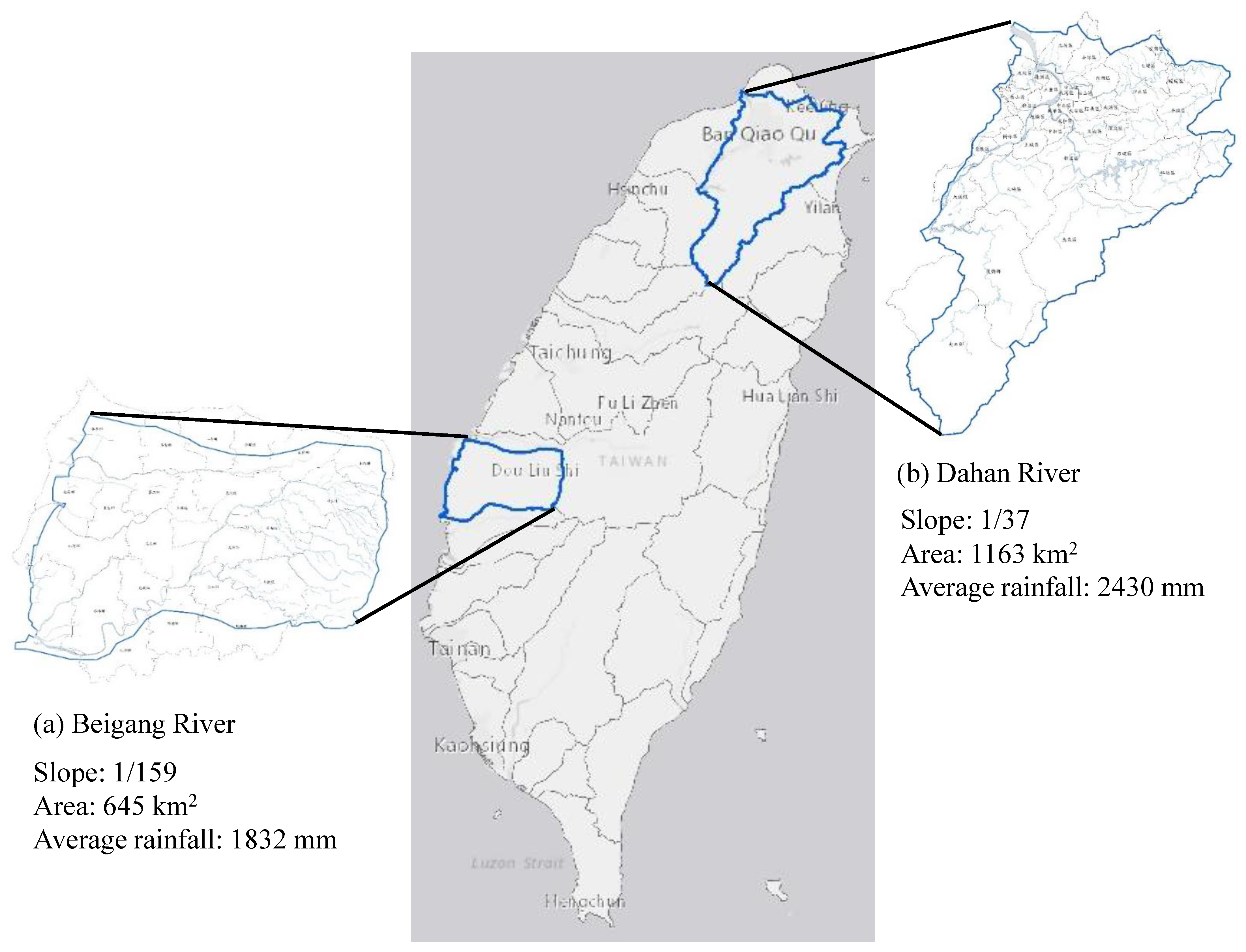
River sedimentation has already attracted much attention all over the world. Moreover, the issue of river erosion and deposition, caused by flooding disasters, is highlighted in Taiwan, an island in East Asia. Among all the rivers in Taiwan, the Beigang and Dahan Rivers, observed to have severe sedimentation problems, were selected to be our investigation field site. The relative locations of the Beigang and Dahan Rivers in Taiwan are shown in Figure 2.
Beigang River was initially one affluent of the Chouishui River. It is about 82 km long and has a drainage area of about 645.2 square kilometers. The river elevation is mostly between 100 and 270 m; the flat area accounts for about 80% of the total area of 516 square kilometers. The slope is between 1/1200 and 1/10,000, from the mountainside to the river estuary. In addition, the average slope of the Beigang River is 1/159. The severe problem of this river is the erodible trend, because of the enormous flood. Therefore, we focus on the variation in the critical cross-section. The selected comparison basis is the measured data of 2000 and 2007.
Dahan River is the main channel of the Shihmen Reservoir, and this reservoir is the major water construction in Northern Taiwan. However, Shimen Reservoir suffered from several serious typhoons and lost 34% of its storage capacity, due to the huge amount of yield sediment from the watershed. In addition, climate change led to the rise in the frequency of extreme flood events. These two factors caused the inflow sediment to increase dramatically. Therefore, this study adopts the Dahan River to investigate the sedimentation issue. The selected comparison basis is the measured data of 2012 and 2013 typhoon events. The case study list is shown in Table 2.
4. Results and Discussion
This research focuses on the ensemble size in the sedimentation simulation. Two different river basins were adopted to determine the feasible ensemble size, by using the variation in the cross-section elevation, sediment concentration, and bed elevation.
4.1. Performance of Bed Elevation Hindcasting
Table 3 shows the simulation performance obtained from different ensemble sizes, from single to 100 in Beigang River. Each estimation standard value shown in Table 3 indicates that each ensemble size presents a reasonable result in bed elevation hindcasting. The RMSE shows the continued downward trend, and the CC and NS present the continued upward trend from single to 100 ensemble size. As a result, the performance is presented with a significantly improving trend with the increasing ensemble size. Regarding the combination of ensemble sizes, the trend of the performance obtained in the ensemble size of 20 is significant compared to that of the single ensemble size. The improvement becomes insignificant when the ensemble size is larger than 20, and an ensemble size of 20 should be the better selection.
Figure 3a shows the simulated results of the 100 ensemble members generated, with the performance from the worst member to the best member, individually. It can be observed that the simulations produce a similar downward trend for RMSE, and an upward trend for CC and NS, and, finally, reach a similar accuracy when the best member is provided. Figure 3b further shows the simulated results of multiple parameters, with the combination of different ensemble sizes, cumulatively. For example, the values at 20 members indicate that the statistical indexes are calculated by combining the outputs obtained from the worst 20 members. By displaying the results in this way, it is easier to find the inflection point that occurs at the member size of 20, in terms of the NS, RMSE, and CC indexes. The results displayed in b indicate the worst scenario for different ensemble sizes, because members are selected in the order of the worst to the best members. In other words, if we randomly select 20 out of the 100 members, the accuracy will undoubtedly be equal to, or better than, the worst 20 members. Moreover, it should be noted that the NS, RMSE, and CC obtained from the single ensemble size are 0.170, 2.393, and 0.529 (see Table 3), respectively. Nevertheless, the NS, RMSE, and CC criteria improve to 0.219, 2.320, and 0.547 when the performance is computed based on 20 members. In addition, the NS, RMSE, and CC criteria improve to 0.233, 2.300, and 0.549 when the performance is computed based on 100 members. By comparing with the above data, the ensemble size of 20 has already obtained a better improvement, and the ensemble size of 100 just obtained a slight improvement.
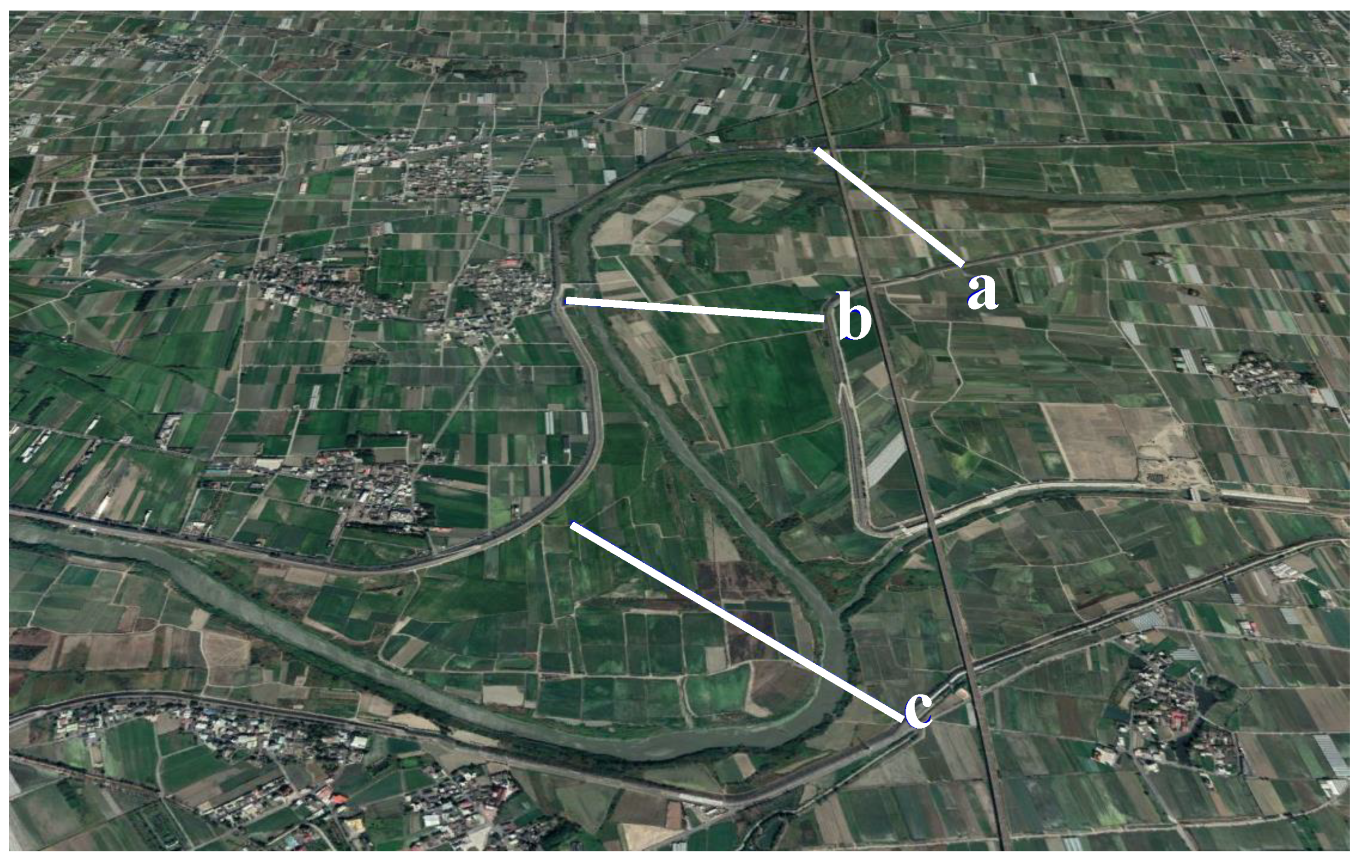
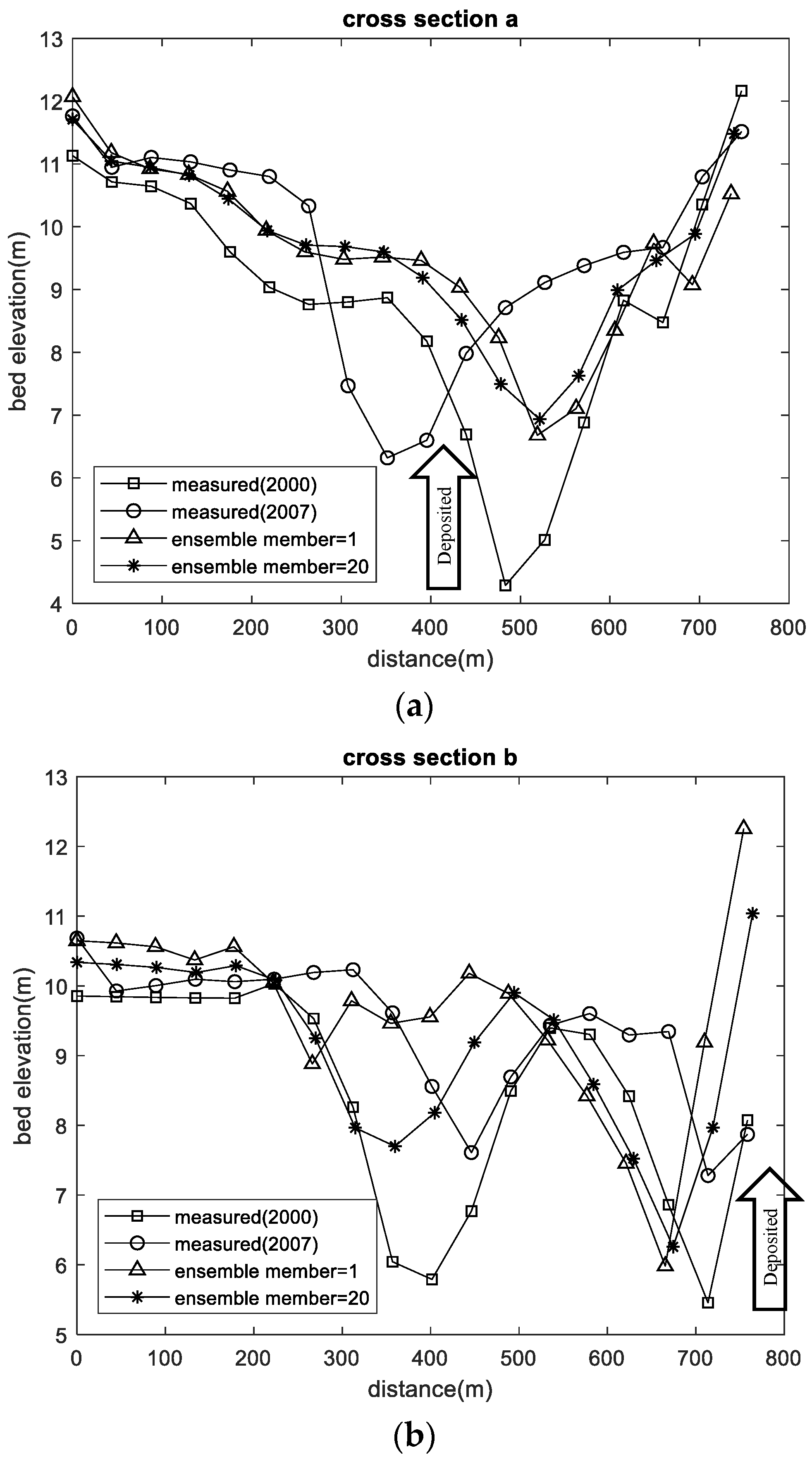
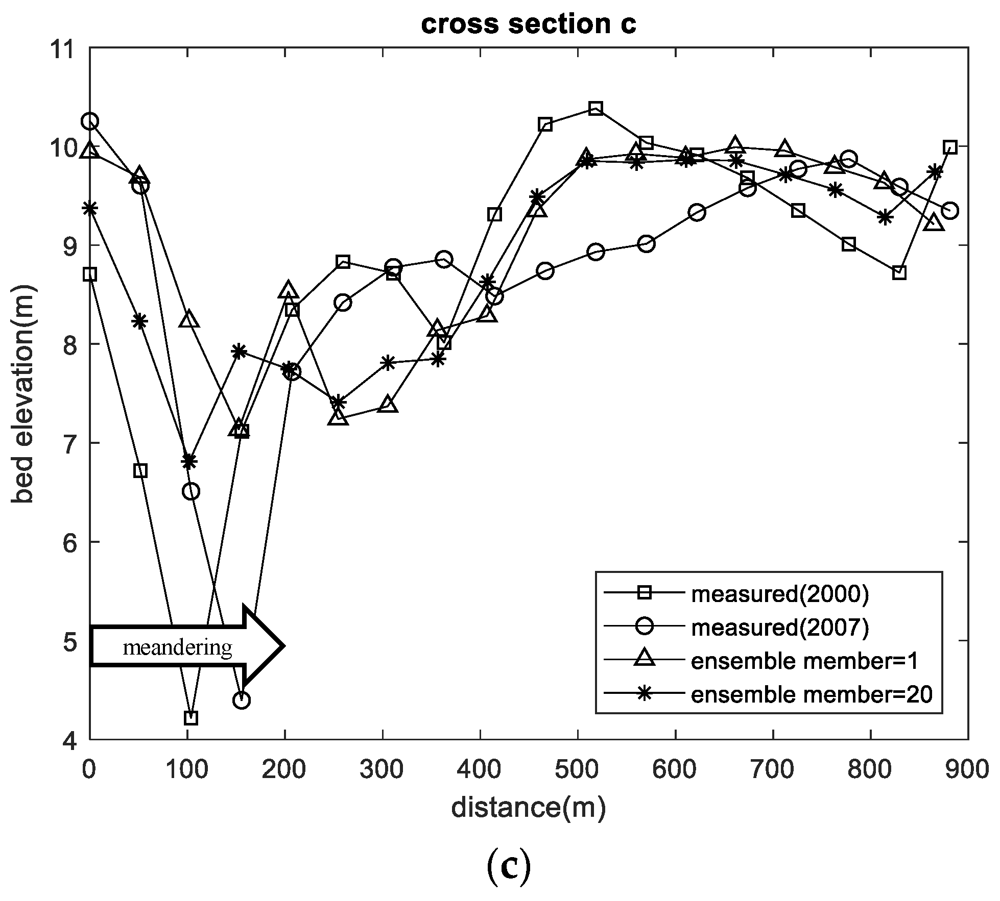
The above indexes are used to evaluate the variation in the river bed elevation in each cross-section. The adopted sections shown in Figure 4 are a, b, and c will be presented in Figure 5. As a result, the simulation results in Figure 5a,b can reflect the deposition trend from the year 2000 to 2007; the simulation of Figure 5c can reflect the variation in river main channel meandering from the year 2000 to 2007. Although the accurate absolute elevation is challenging to be simulated, the clear trend indicates that the ensemble size of 20 has already presented a good improvement ability. The above information is sufficient to help the management to organize a feasible strategy.
4.2. Performance of Sediment Concentration Hindcasting
Table 4 and Figure 6 show the simulation performance obtained from different ensemble sizes, from single to 100, by different sediment formulas. Each estimation standard value shown in Table 4 indicates that each ensemble size presents a continued improving trend in sediment concentration hindcasting. The CC and NS present the upward trend, and the RMSE presents the downward trend as the ensemble size increases. Regarding the combination of ensemble sizes, the trend of the performance obtained in the ensemble size of 20 is significant compared to that of the single ensemble size. The improvement becomes insignificant when the ensemble size is larger than 20. It is clear that the ensemble size of 20 should be the better selection.
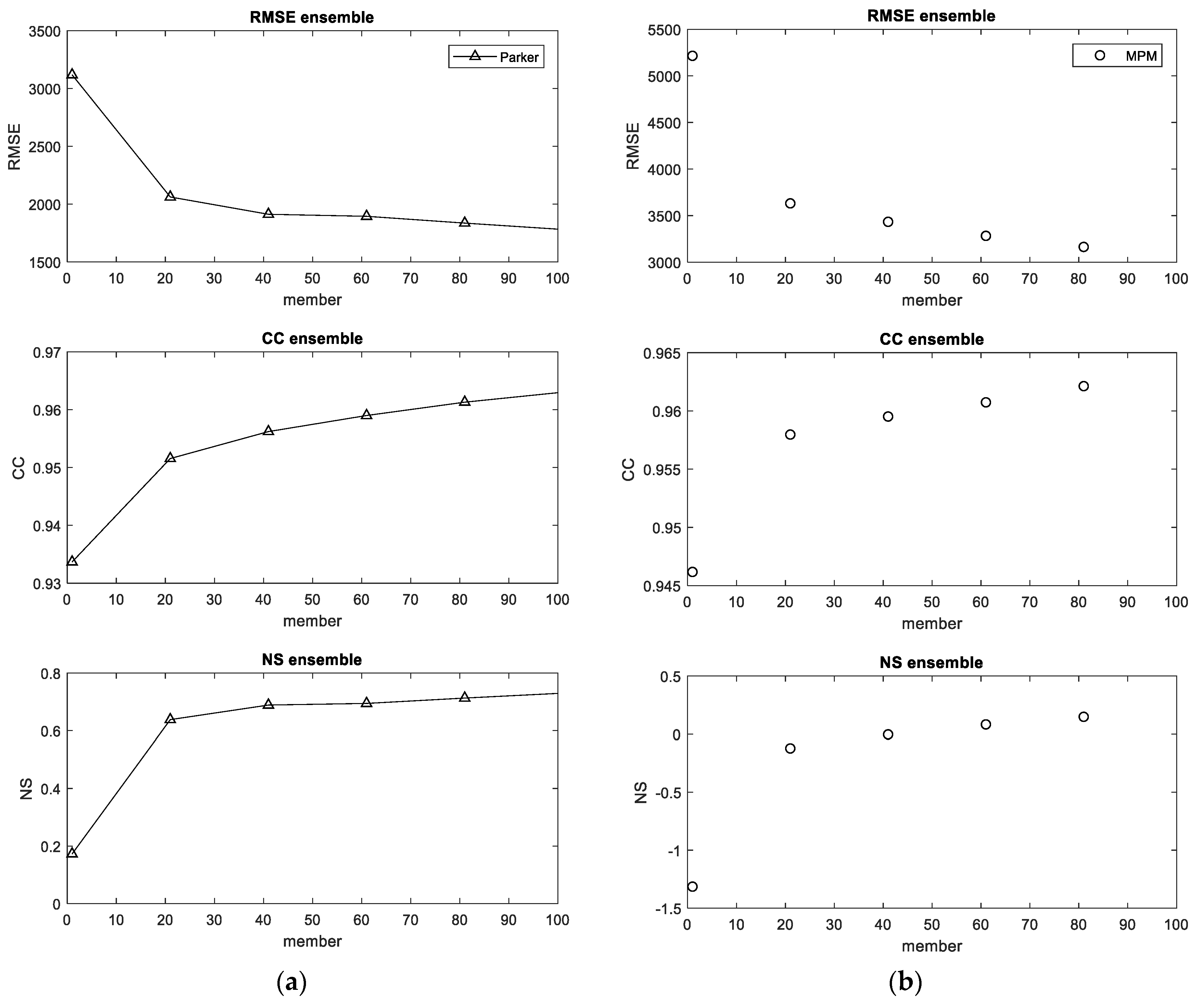
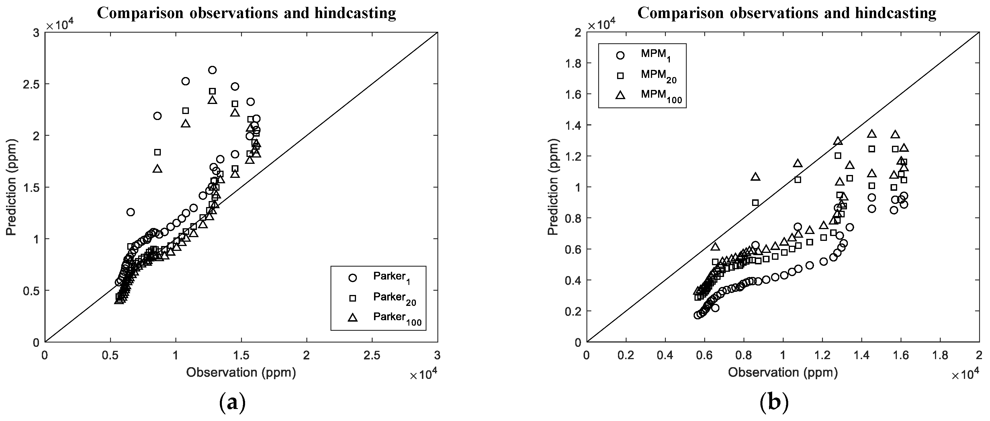
Figure 7 shows a scatter plot of observation and prediction. It is clear that prediction obtained a reasonable result, and models with a larger ensemble size are closer to the ideal (1:1) line. Overall, the Parker formula presents an underestimation trend; in contrast, the MPM formula indicates an overestimation pattern. The importance is that both sediment formulae can show higher accuracy when the sediment concentration is between 6000 and 8000 ppm. In addition, the scatter points of the ensemble size of 20 almost coincide with the ensemble size of 100.
Figure 8 shows the comparison of the simulated and observed sediment concentration variations by using different sediment formulas. The forecasting interval (FI) indicates the uncertainty of the model outputs. The interval produced by all 100 members is provided (grey) to show the reliability of model hindcasting. For Parker (Figure 8a), the whole journey simulation produces similar results and performs well compared with the observation. For MPM (Figure 8b), the simulated result presents a similar trend to the observation. The relative error value is slightly higher than the Parker; However, it indicates that the result is consistent. In addition, the differences in the outcomes between Parker (1990) and MPM (2006) is due to the riverbed material.
4.3. Determination of Ensemble Size
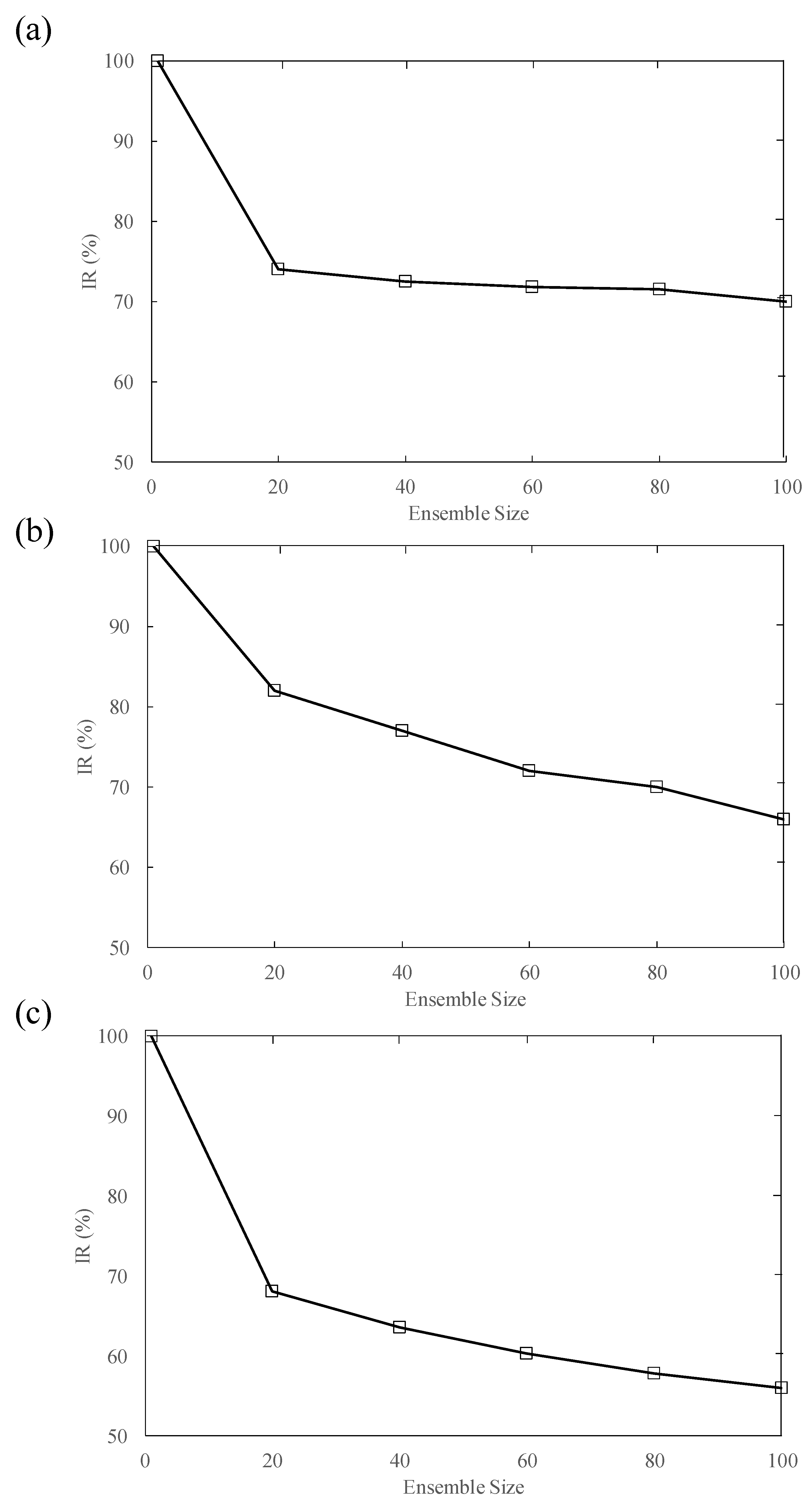
Figure 9 shows the performance of cross-section elevation, sediment concentration, and bed elevation by different ensemble sizes. The results obtained from different cases with 20 members are quite similar to those for 100 members, indicating that members above 20 are redundant and the improvement is also limited. As far as the accuracy and efficiency are concerned, there should be a trade-off when calibrating sediment transport simulation models. It usually takes more computational time (less efficient) for calibration or training if the model requires better hindcasting (more accurate), and vice versa. The results obtained in the present study suggest that for the single model fusion multiple parameter combination, the ensemble size 20 provides a good compromise between model accuracy and efficiency. In addition, the improvement is insignificant, but there is an increase in simulation time when the ensemble size is larger than 20. For example, an ensemble size of 100 will increase the simulation time to 5 times, and it is detrimental to apply this to forecasting work.
5. Concluding Remarks
The purpose of this research is to embed the ensemble method concept to improve the forecasting ability to respond to extreme disasters. This study firstly combines the ensemble method concepts and the sediment transport simulation to figure out the applicability of ensemble members. This study proposes a multiple parameter combination in a single model, to analyze the sensitivity of ensemble size by evaluation of their efficiency and accuracy for river sediment concentration, bed elevation, and erodible trend. Firstly, 100 members were generated, respectively, with different parameter combinations for the optimal ensemble size.
The results indicate that multiple parameter combinations do contribute to river sedimentation hindcasting, because the accuracy of SRH-2D is enhanced as the number of ensemble members is increased. The inflection of the improvement rate occurring at the ensemble size of 20 shows that the improvement as the ensemble size number rises from 1 to 20 is much higher than the improvement as the number goes from 20 to 100. In terms of model accuracy and efficiency, the ensemble size of 20 can provide a compromised solution between model accuracy and simulation time.
Finally, this study gives a detailed and complete investigation of the suitability of the ensemble size for the sediment transport numerical model. The performance demonstrates that 20 ensemble members are sufficient to describe the variation in river sedimentation, and can provide reliable hindcasting of sediment concentration, and the erosion and deposition trend. In other words, the ensemble method can reduce the uncertainty of model parameters, to improve reliability. It is urgent and necessary for an advanced early warning system.
The generalization or suitability of ensemble size for different problems, such as rainfall forecasting and water quality simulation, have not been verified. The determined ensemble size, 20, can be a valuable reference to further investigate these issues.
Author Contributions
Conceptualization, H.-C.H.; methodology, H.-C.H. and Y.-M.C.; software, C.-C.L.; validation, C.-C.L., Y.-M.C. and C.-C.H.; formal analysis, H.-C.H., H.-Y.L. and C.-C.H.; investigation, H.-C.H., C.-C.L. and C.-C.H.; resources, H.-C.H. and H.-Y.L.; data curation, H.-C.H. and C.-C.H.; writing—original draft preparation, C.-C.L. and C.-C.H.; writing—review and editing, H.-C.H. and C.-C.H.; supervision, H.-Y.L. and Y.-M.C.; project administration, H.-C.H. and H.-Y.L.; funding acquisition, H.-C.H. All authors have read and agreed to the published version of the manuscript.
Funding
Ministry of Science and Technology (109-2621-M-002-004-); National Taiwan University (NTU-108L8806).
Institutional Review Board Statement
Not applicable.
Informed Consent Statement
Not applicable.
Data Availability Statement
Not applicable.
Conflicts of Interest
The authors declare no conflict of interest.
Nomenclature
| model constant and the default value = 0.7 is used in this study | |
| average particle size. | |
| median diameter (m) | |
| average water depth | |
| the RMSE obtained from the single model | |
| the RMSE obtained from the multiple parameters combination averaging | |
| acceleration of gravity | |
| water depth | |
| turbulent kinetic energy | |
| bed load constants | |
| bed load constants | |
| manning’s coefficient | |
| volume of particle distribution in active layer fraction and | |
| volume of particle distribution in sub-surface fraction | |
| erosion rate potential | |
| unit sediment discharge (ton/m) | |
| the observed value | |
| the hindcast value | |
| the means of hindcast value | |
| hydraulic radius (m) | |
| energy slope | |
| , , | depth-averaged stresses due to turbulence and dispersion |
| time | |
| depth-averaged velocity in -direction | |
| bed frictional velocity | |
| depth-averaged velocity in -direction | |
| average velocity | |
| -direction in Cartesian coordinate | |
| -direction in Cartesian coordinate | |
| water surface elevation | |
| bed elevation | |
| water density | |
| sediment density | |
| bed shear stress | |
| bed shear stresses in -direction | |
| bed shear stresses in -direction | |
| particle shear stress; | |
| kinematic viscosity of water | |
| eddy viscosity | |
| active layer thickness, which is the sensitive parameter in sedimentation simulation | |
| sub-surface layer thickness |
References
- Lai, Y.G.; Wu, K. Modeling of vertical and lateral erosion on the Chosui River, Taiwan. In Proceedings of the World Environmental and Water Resources Congress 2013: Showcasing the Future, Cincinnati, OH, USA, 19–23 May 2013; pp. 1747–1756. [Google Scholar]
- Lai, Y.G.; Wu, K. Combined Vertical And Lateral Channel Evolution Numerical Modeling. In Proceedings of the 11th International Conference on Hydroinformatics HIC 2014, New York, NY, USA, 17–21 August 2014. [Google Scholar]
- Moges, E.M. Evaluation of Sediment Transport Equations and Parameter Sensitivity Analysis Using the SRH-2D Model. Master’s Thesis, Universität Stuttgart, Stuttgart, Germany, 2010. [Google Scholar]
- Greimann, B.; Sheydayi, P.; Vargas, S.; Lai, Y.; Mefford, B. Developing Mitigation Plans for Matilija Dam Removal. In Proceedings of the World Environmental and Water Resources Congress 2008: Ahupua’A, Honolulu, HI, USA, 12–16 May 2008; pp. 1–9. [Google Scholar]
- Huang, J.; Russell, K. Two-dimensional numerical simulation of a Grand Canyon sandbar during a high flow experiment. In Proceedings of the World Environmental and Water Resources Congress 2014: Water without Borders, Portland, OR, USA, 1–5 June 2014; pp. 1183–1190. [Google Scholar]
- Ajami, N.K.; Duan, Q.; Sorooshian, S. An integrated hydrologic Bayesian multimodel combination framework: Confronting input, parameter, and model structural uncertainty in hydrologic prediction. Water Resour. Res. 2007, 43. [Google Scholar] [CrossRef]
- Beven, K. A manifesto for the equifinality thesis. J. Hydrol. 2000, 6, 18–36. [Google Scholar] [CrossRef] [Green Version]
- Beven, K.; Binley, A. The future of distributed models: Model calibration and uncertainty prediction. Hydrol. Process. 1992, 6, 279–298. [Google Scholar] [CrossRef]
- Kuczera, G.; Parent, E. Monte Carlo assessment of parameter uncertainty in conceptual catchment models: The Metropolis algorithm. J. Hydrol. 1998, 211, 69–85. [Google Scholar] [CrossRef]
- Vrugt, J.A.; Gupta, H.V.; Bouten, W.; Sorooshian, S. A Shuffled Complex Evolution Metropolis algorithm for optimization and uncertainty assessment of hydrologic model parameters. Water Resour. Res. 2003, 39, 1201. [Google Scholar] [CrossRef] [Green Version]
- Montanari, A.; Brath, A. A stochastic approach for assessing the uncertainty of rainfall-runoff simulations. Water Resour. Res. 2004, 40, W01106. [Google Scholar] [CrossRef]
- Kitanidis, P.K.; Bras, R.L. Adaptive filtering through detection of isolated transient errors in rainfall-runoff models. Water Resour. Res. 1980, 16, 740–748. [Google Scholar] [CrossRef]
- Kitanidis, P.K.; Bras, R.L. Real-time forecasting with a conceptual hydrologic model: 2. Applications and results. Water Resour. Res. 1980, 16, 1034–1044. [Google Scholar] [CrossRef]
- Beck, M.B. Water quality modeling: A review of the analysis of uncertainty. Water Resour. Res. 1987, 23, 1393–1442. [Google Scholar] [CrossRef] [Green Version]
- Evensen, G. Using the extended Kalman filter with a multilayer quasi-geostrophic ocean model. J. Geophys. Res. Ocean. 1992, 97, 17905–17924. [Google Scholar] [CrossRef] [Green Version]
- Miller, R.N.; Ghil, M.; Gauthiez, F. Advanced data assimilation in strongly nonlinear dynamical systems. J. Atmos. Sci. 1994, 51, 1037–1056. [Google Scholar] [CrossRef]
- Moradkhani, H.; Hsu, K.L.; Gupta, H.; Sorooshian, S. Uncertainty assessment of hydrologic model states and parameters: Sequential data assimilation using the particle filter. Water Resour. Res. 2005, 41. [Google Scholar] [CrossRef] [Green Version]
- Shamseldin, A.Y.; O’Connor, K.M.; Liang, G.C. Methods for combining the outputs of different rainfall–runoff models. J. Hydrol. 1997, 197, 203–229. [Google Scholar] [CrossRef]
- Abrahart, R.J.; See, L. Multi-model data fusion for river flow forecasting: An evaluation of six alternative methods based on two contrasting catchments. Hydrol. Earth Syst. Sci. Discuss. 2002, 6, 655–670. [Google Scholar] [CrossRef] [Green Version]
- Georgakakos, K.P.; Seo, D.J.; Gupta, H.; Schaake, J.; Butts, M.B. Towards the characterization of streamflow simulation uncertainty through multimodel ensembles. J. Hydrol. 2004, 298, 222–241. [Google Scholar] [CrossRef]
- Ajami, N.K.; Duan, Q.; Gao, X.; Sorooshian, S. Multimodel combination techniques for analysis of hydrological simulations: Application to distributed model intercomparison project results. J. Hydrometeorol. 2006, 7, 755–768. [Google Scholar] [CrossRef]
- Ajami, N.K.; Duan, Q.; Moradkhni, H.; Sorooshian, S. 1.3. Recursive Bayesian model combination for streamflow forecasting. In Proceedings of the American Meteorological Society Meeting, San Diego, CA, USA, 9–13 January 2005. [Google Scholar]
- Hoeting, J.A.; Madigan, D.; Raftery, A.E.; Volinsky, C.T. Bayesian model averaging: A tutorial. Stat. Sci. 1999, 14, 382–401. [Google Scholar]
- Thiboult, A.; Anctil, F.; Boucher, M.A. Accounting for three sources of uncertainty in ensemble hydrological forecasting. Hydrol. Earth Syst. Sci. 2016, 20, 1809–1825. [Google Scholar] [CrossRef] [Green Version]
- Alfieri, L.; Burek, P.; Dutra, E.; Krzeminski, B.; Muraro, D.; Thielen, J.; Pappenberger, F. GloFAS-global ensemble streamflow forecasting and flood early warning. Hydrol. Earth Syst. Sci. 2013, 17, 1161–1175. [Google Scholar] [CrossRef] [Green Version]
- Duan, Q.; Ajami, N.K.; Gao, X.; Sorooshian, S. Multi-model ensemble hydrologic prediction using Bayesian model averaging. Adv. Water Resour. 2007, 30, 1371–1386. [Google Scholar] [CrossRef] [Green Version]
- Leutbecher, M.; Palmer, T.N. Ensemble forecasting. J. Comput. Phys. 2008, 227, 3515–3539. [Google Scholar] [CrossRef]
- Jiang, S.H.; Ren, L.I.; Yang, X.I.; Ma, M.I.; Liu, Y. Multi-model ensemble hydrologic prediction and uncertainties analysis. Proc. Int. Assoc. Hydrol. Sci. 2014, 364, 249–254. [Google Scholar] [CrossRef]
- Tiwari, M.K.; Chatterjee, C. Uncertainty assessment and ensemble flood forecasting using bootstrap based artificial neural networks (BANNs). J. Hydrol. 2010, 382, 20–33. [Google Scholar] [CrossRef]
- Napolitano, G.; Serinaldi, F.; See, L. Impact of EMD decomposition and random initialisation of weights in ANN hindcasting of daily stream flow series: An empirical examination. J. Hydrol. 2011, 406, 199–214. [Google Scholar] [CrossRef]
- Chiang, Y.M.; Hao, R.N.; Ho, H.C.; Chang, T.J.; Xu, Y.P. Evaluating the contribution of multi-model combination to streamflow hindcasting by empirical and conceptual models. Hydrol. Sci. J. 2017, 62, 1456–1468. [Google Scholar] [CrossRef]
- Lai, Y.G.; Thomas, R.E.; Ozeren, Y.; Simon, A.; Greimann, B.P.; Wu, K. Coupling a two-dimensional model with a deterministic bank stability model. In Proceedings of the World Environmental and Water Resources Congress 2012: Crossing Boundaries, Albuquerque, NM, USA, 20–24 May 2012; pp. 1290–1300. [Google Scholar]
- Lai, Y.G. SRH-2D Version 2: Theory and User’s Manual. Sedimentation and River Hydraulics–Two-Dimensional River Flow Modeling; US Department of Interior, Bureau of Reclamation: Denver, CO, USA, 2008.
- Pasternack, G.B.; Hopkins, C.E. Near-Census 2D Model Comparison between SRH-2D and TUFLOW GPU for Use in Gravel/Cobble Rivers; University of California at Davis, Prepared for Yuba County Water Agency: Davis, CA, USA, 2017. [Google Scholar]
- Huang, C.C.; Lai, Y.G.; Lai, J.S.; Tan, Y.C. Field and numerical modeling study of turbidity current in Shimen Reservoir during typhoon events. J. Hydraul. Eng. 2019, 145, 05019003. [Google Scholar] [CrossRef]
- Huang, C.C.; Lin, W.C.; Ho, H.C.; Tan, Y.C. Estimation of Reservoir Sediment Flux through Bottom Outlet with Combination of Numerical and Empirical Methods. Water 2019, 11, 1353. [Google Scholar] [CrossRef] [Green Version]
- AlQasimi, E.; Mahdi, T.F. Rivers’ Confluence Morphological Modeling Using SRH-2D. In Advances in Natural Hazards and Hydrological Risks: Meeting the Challenge; Springer: Berlin/Heidelberg, Germany, 2020; pp. 171–176. [Google Scholar]
- Lai, Y.G.; Greimann, B.P. Predicting contraction scour with a two-dimensional depth averaged model. J. Hydraulic. Res. 2010, 48, 383–387. [Google Scholar] [CrossRef]
- Meyer-Peter, E.; Müller, R. Formulas for Bed-Load Transport; IAHSR 2nd Meeting; appendix 2; IAHR: Stockholm, Sweden, 1948. [Google Scholar]
- Parker, G. Surface-based bedload transport relation for gravel rivers. J. Hydraul. Res. 1990, 28, 417–436. [Google Scholar] [CrossRef]
Figure 1.
Flowchart of the proposed approach.
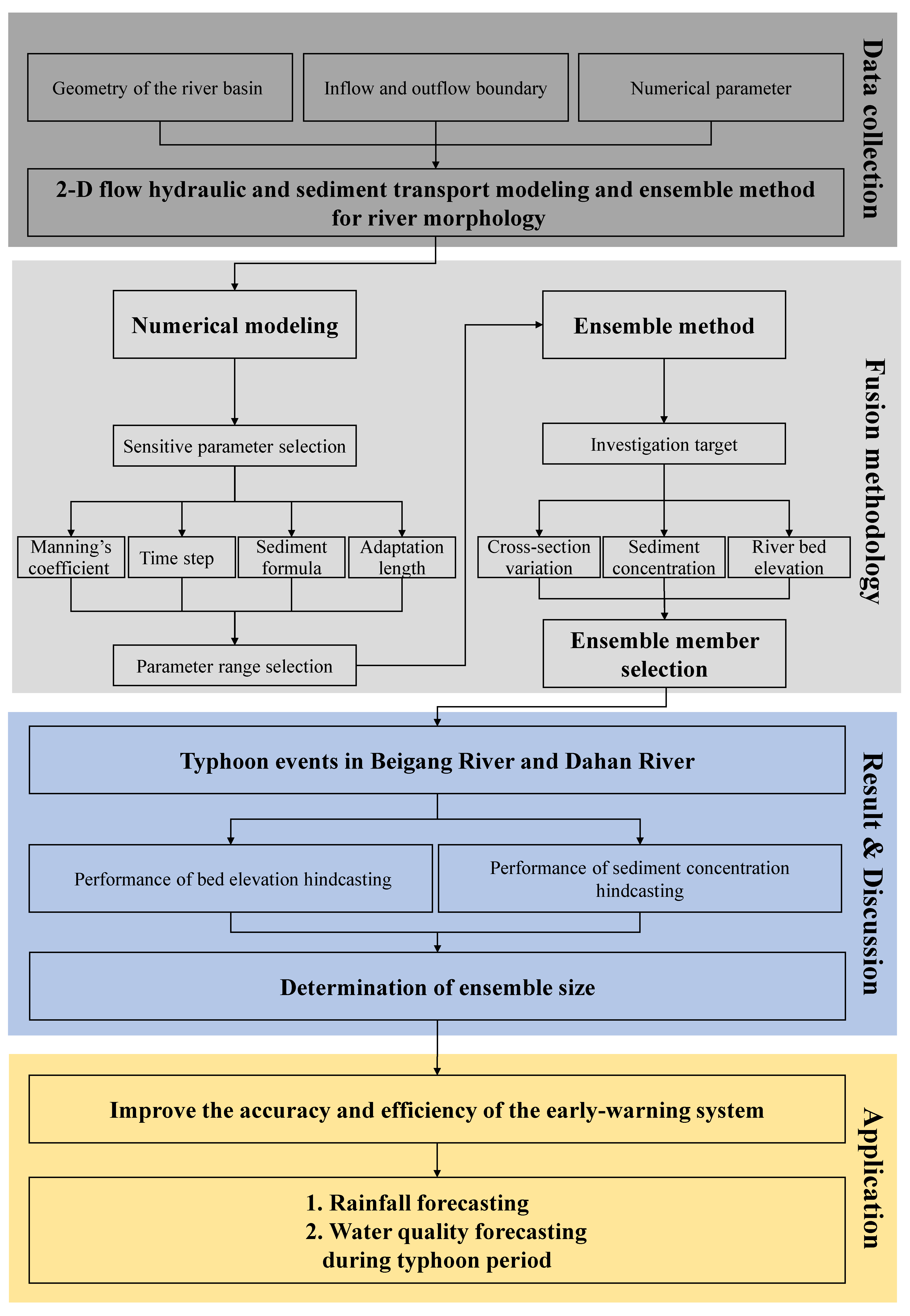
Figure 2.
Location of the (a) Beigang River; (b) Dahan River.

Figure 3.
Simulation performance obtained from (a) individual member; (b) different ensemble sizes in Beigang River.
Figure 3.
Simulation performance obtained from (a) individual member; (b) different ensemble sizes in Beigang River.
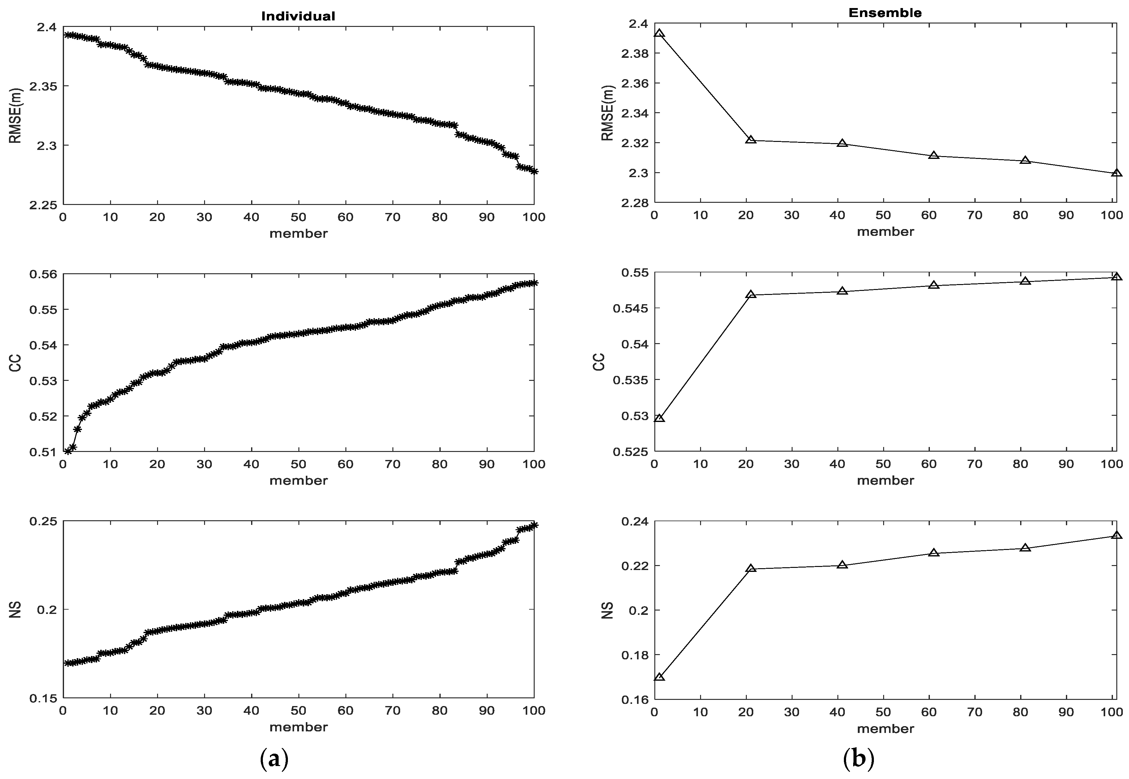
Figure 4.
Simulation zone and compared cross-section (a–c) of Beigang River.

Figure 5.
Comparison of the measurement and the simulation obtained from different ensemble sizes of (a–c) in Beigang River.
Figure 5.
Comparison of the measurement and the simulation obtained from different ensemble sizes of (a–c) in Beigang River.


Figure 6.
Comparison of prediction and observation obtained from different ensemble sizes in Dahan River, (a) Parker; (b) MPM.
Figure 6.
Comparison of prediction and observation obtained from different ensemble sizes in Dahan River, (a) Parker; (b) MPM.

Figure 7.
Simulation performance obtained from different ensemble sizes in Dahan River, (a) Parker; (b) MPM.
Figure 7.
Simulation performance obtained from different ensemble sizes in Dahan River, (a) Parker; (b) MPM.

Figure 8.
Comparison of the simulated and measured data, (a) Parker; (b) MPM.
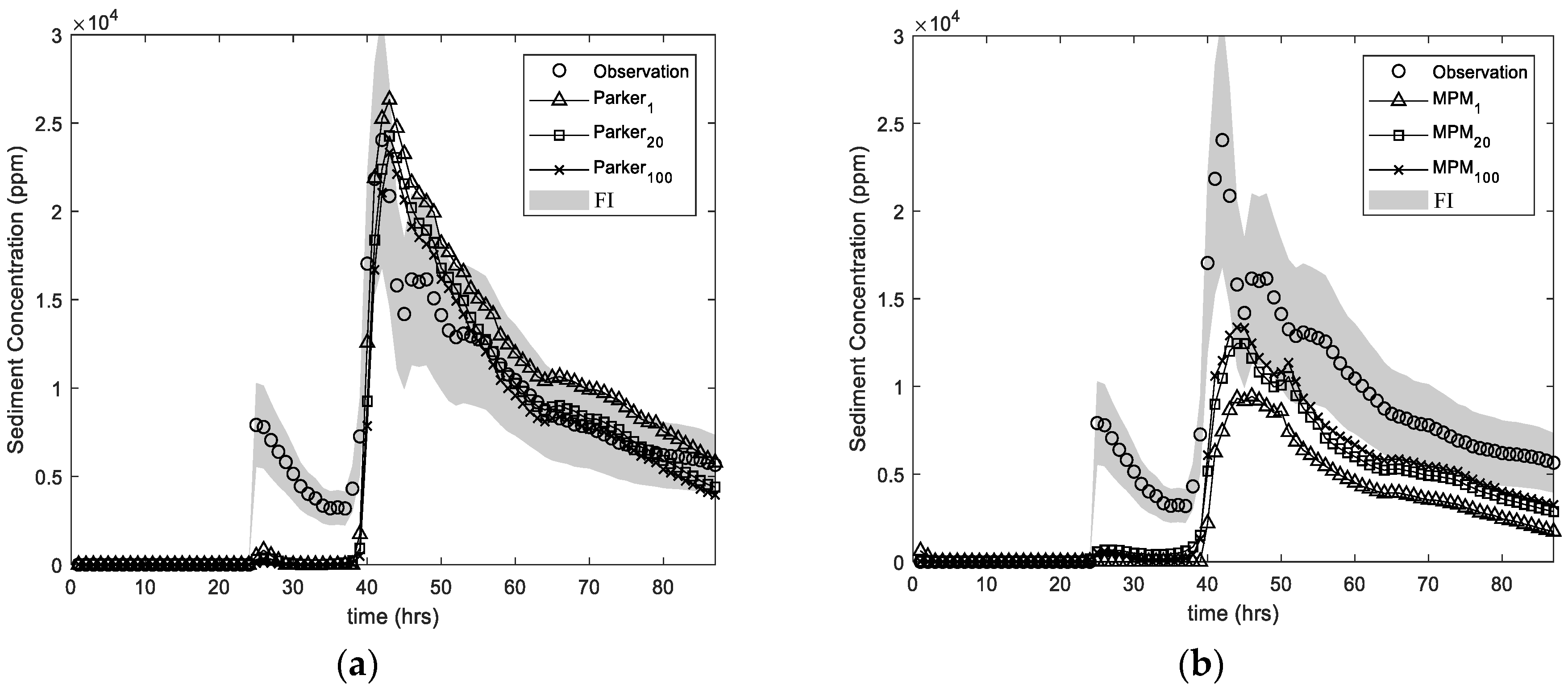
Figure 9.
Performance of (a) cross-section elevation; (b) sediment concentration; (c) bed elevation by different ensemble sizes.
Figure 9.
Performance of (a) cross-section elevation; (b) sediment concentration; (c) bed elevation by different ensemble sizes.


Table 1.
Parameter range selection.
| Term | Manning’s Coefficient | Time Step | Sediment Formula | Adaptation Length |
|---|---|---|---|---|
| Range | 0.015–0.050 | 0.5–2.5 (s) | MPM (1948), and Parker (1990) | 1 to 5 times river width |
Table 2.
Case study list.
| Region | Event Duration (h) | Initial Condition | Target |
|---|---|---|---|
| Beigang | 2000–2007 typhoons | 2000 bed elevation | Cross-section variation |
| Dahan | 2012–2013 typhoons | 2012 bed elevation | Sediment concentration, river bed elevation |
Table 3.
Performance by different ensemble size in Beigang River.
| Region | Beigang River | ||
|---|---|---|---|
| RMSE(m) | CC | NS | |
| single | 2.393 | 0.529 | 0.170 |
| 20 | 2.320 | 0.547 | 0.219 |
| 40 | 2.321 | 0.548 | 0.220 |
| 60 | 2.311 | 0.548 | 0.226 |
| 80 | 2.309 | 0.549 | 0.227 |
| 100 | 2.300 | 0.549 | 0.233 |
Table 4.
Simulation performance obtained from different ensemble size in Dahan River.
| Region | Parker (1990) | MPM (2006) | ||||
|---|---|---|---|---|---|---|
| RMSE(m) | CC | NS | RMSE(m) | CC | NS | |
| single | 3118 | 0.934 | 0.173 | 5215 | 0.946 | 0.032 |
| 20 | 2060 | 0.951 | 0.639 | 3642 | 0.958 | 0.045 |
| 40 | 1907 | 0.956 | 0.691 | 3442 | 0.959 | 0.062 |
| 60 | 1894 | 0.959 | 0.69 | 3290 | 0.963 | 0.079 |
| 80 | 1838 | 0.961 | 0.713 | 3169 | 0.962 | 0.145 |
| 100 | 1785 | 0.963 | 0.73 | 3070 | 0.963 | 0.198 |
Publisher’s Note: MDPI stays neutral with regard to jurisdictional claims in published maps and institutional affiliations. |
© 2021 by the authors. Licensee MDPI, Basel, Switzerland. This article is an open access article distributed under the terms and conditions of the Creative Commons Attribution (CC BY) license (https://creativecommons.org/licenses/by/4.0/).
Share and Cite
MDPI and ACS Style
Ho, H.-C.; Chiang, Y.-M.; Lin, C.-C.; Lee, H.-Y.; Huang, C.-C. Development of an Interdisciplinary Prediction System Combining Sediment Transport Simulation and Ensemble Method. Water 2021, 13, 2588. https://doi.org/10.3390/w13182588
AMA Style
Ho H-C, Chiang Y-M, Lin C-C, Lee H-Y, Huang C-C. Development of an Interdisciplinary Prediction System Combining Sediment Transport Simulation and Ensemble Method. Water. 2021; 13(18):2588. https://doi.org/10.3390/w13182588
Chicago/Turabian StyleHo, Hao-Che, Yen-Ming Chiang, Che-Chi Lin, Hong-Yuan Lee, and Cheng-Chia Huang. 2021. "Development of an Interdisciplinary Prediction System Combining Sediment Transport Simulation and Ensemble Method" Water 13, no. 18: 2588. https://doi.org/10.3390/w13182588
Note that from the first issue of 2016, this journal uses article numbers instead of page numbers. See further details here.