
Efficient Hazard Assessment for Pluvial Floods in Urban Environments: A Benchmarking Case Study for the City of Berlin, Germany


Institute of Environmental Science and Geography, University of Potsdam, 14476 Potsdam, Germany
*
Author to whom correspondence should be addressed.
Water 2021, 13(18), 2476; https://doi.org/10.3390/w13182476
Submission received: 14 August 2021
/
Revised: 3 September 2021
/
Accepted: 7 September 2021
/
Published: 9 September 2021
(This article belongs to the Special Issue Assessment and Management of Flood Risk in Urban Areas)
Abstract
:The presence of impermeable surfaces in urban areas hinders natural drainage and directs the surface runoff to storm drainage systems with finite capacity, which makes these areas prone to pluvial flooding. The occurrence of pluvial flooding depends on the existence of minimal areas for surface runoff generation and concentration. Detailed hydrologic and hydrodynamic simulations are computationally expensive and require intensive resources. This study compared and evaluated the performance of two simplified methods to identify urban pluvial flood-prone areas, namely the fill–spill–merge (FSM) method and the topographic wetness index (TWI) method and used the TELEMAC-2D hydrodynamic numerical model for benchmarking and validation. The FSM method uses common GIS operations to identify flood-prone depressions from a high-resolution digital elevation model (DEM). The TWI method employs the maximum likelihood method (MLE) to probabilistically calibrate a TWI threshold () based on the inundation maps from a 2D hydrodynamic model for a given spatial window (W) within the urban area. We found that the FSM method clearly outperforms the TWI method both conceptually and effectively in terms of model performance.
1. Introduction
Pluvial flooding causes massive human and economic losses [1,2]. They are considered as an omnipresent hazard both in urban and rural areas, e.g., [3,4]. Pluvial floods are caused by intensive and short duration precipitation storms due to the limited capacity of storm drainage systems, typically called “minor systems”, which result in the generation of overland flow that travels through the terrain, depressions and the road networks, creating a surface flow network typically called the “major system”. The major system could transfer the overland flow for a long distance, which can cause flooding in an area that is located far from the location where the minor system’s capacity was exceeded [5,6].
Pluvial flood-prone areas can be defined as the low elevated areas within the urban watershed where excess runoff accumulates [7]. It is challenging to predict pluvial floods as they could strike areas with no flood records with little warning time. They have no defined flood plains such as rivers and seashores [8]. Furthermore, they depend on how well the storm drainage system and the associated infrastructure respond to a sudden precipitation storm. The damage depends not only on the event intensity and duration but also on physical and social urban characteristics [9,10,11]. The European Flood Directive widely implements flood hazard maps for rivers and coastal areas, but corresponding efforts are scarce for pluvial flooding [8,12,13].
Urban pluvial floods are affected by several local factors, for example, the presence and maintenance conditions of the storm drainage system, the existence of underground infrastructures, and the extent of impervious surfaces within the urban watershed [8]. Sustainable urban development requires efficient pluvial flood modeling [14]. Urban pluvial flood hazard mapping is commonly carried out by performing hydrologic modeling to estimate the excess runoff followed by a 1D-2D hydrodynamic simulation to compute the inundation extent and depth and runoff velocity. This method is considered the most accurate representation of the storm drainage system. However, this method is computationally expensive, requires comprehensive knowledge of hydrology and hydraulics, as well as detailed input data such as topography, land cover, soil type, and storm drainage system data, which hamper its widespread application in a large urban watershed for pluvial flood hazard mapping and early warnings [15,16,17].
In recent years, the increasing availability of higher resolution DEM has encouraged not only the advanced application of the 2D hydrodynamic models but also the development of quick and simplified methods that are based on DEM as valid alternatives for flood hazard mapping. These simplified methods have been mainly developed and applied for mapping fluvial flood hazards, and their application for pluvial flooding hazard mapping is still sparse in the literature [18]. They are less accurate than using detailed hydrologic and 1D-2D hydrodynamic models, but they are faster and require fewer input data. Therefore, they are suitable for flood hazard mapping and early warnings for urban areas. Many of the simplified models are based on the fill–spill–merge (FSM) concept where the excess runoff concentrates in the DEM depressions and when a depression is completely filled with excess runoff, the excess runoff spills, and flows downstream towards lower elevated depressions. References [14,18,19] applied the FSM method to different case studies in China, Italy, and Denmark. FSM can map the pluvial flood hazard in urban watersheds quickly as it only shows the final inundation extent. Reference [18] evaluated the FSM method performance based on evaluating the estimated inundation area extent with the obtained inundation area extent from a 2D hydrodynamic model. However, they did not evaluate the water depth, which is vital for damage assessment. Therefore, this study evaluates the FSM method performance based on both flood extent and the water depth for pluvial flooding.
Other previous studies proposed methods to delineate flood-prone areas based on geomorphic classifiers [20,21,22]. They are suitable for data-scarce regions and to analyze large geographic regions that have limited information on flooding potential. Reference [23] showed that urban flood reported areas tend to have high TWI values and suggested using the TWI as an index for urban pluvial flooding. On the contrary, Reference [24] showed that TWI failed to map the urban pluvial flooding and proposed a DEM-based index to map the urban pluvial flooding, namely the topographic control index (TCI). References [25,26,27] proposed a framework for identifying urban flood-prone areas based on TWI. The framework (hereafter, the TWI method) uses the maximum likelihood method (MLE) to probabilistically calibrate the TWI threshold () based on the inundation maps from a 2D hydrodynamic model for a given spatial window (W) within the urban area, where areas with TWI values that exceed the TWI threshold () are defined as flood-prone areas.
The objective of this study is to evaluate and compare the FSM method and the TWI method to assess and map pluvial flooding and highlight the limitations of each method. We applied the two methods to two urban areas in Berlin for different precipitation depths ranging from 30 to 150 mm (10 mm increments) and used the TELEMAC-2D hydrodynamic numerical model for benchmarking and validation to show how these methods can mimic the behavior of a 2D-hydrodynamic model with regard to inundation depth and inundation extent. Finally, we discuss the advantages and limitations of each method.
2. Data
The high-resolution DEM was downloaded from Berlin’s city geographical information systems spatial databases [28]. The DEM has a 1 × 1 m horizontal resolution and 20 cm vertical accuracy, as shown in Figure 1a. The soil type, hydrologic condition [29] and land use data from open street map [30] were used to generate the curve number map. Furthermore, the radar precipitation data for the period between 2005 and 2019 were obtained from the German Weather Service (DWD) [31,32].
3. Models
3.1. Two-Dimensional Hydrodynamic Simulations
We used the TELEMAC-2D model to perform the 2D hydrodynamic simulations. The TELEMAC-2D model [33,34] is an open-source model and included in the TELEMAC-MASCARET suite. It solves the shallow water equations using both the finite volume method (FVM) and the finite element method (FEM) over non-structured triangular grids. Urban flood inundation mapping is considered a challenge because of the complex characteristics of the urban watersheds. Buildings are known as one of the most significant components of urban flood modeling because they withstand the flow of excess runoff. Reference [35] showed that the building resistance (BR) method is the best representation of buildings in numerical models. The BR method is based on assigning a high roughness coefficient value to the buildings to allow excess runoff to flow through the buildings. Furthermore, the roughness coefficient is also a significant uncertainty factor in urban flood modeling. In the current study, the Manning roughness coefficient was defined based on the surface type as follows: m−1/3· s for buildings and 0.013 for other surface types [36,37,38].
The Blue Kenue software was used to define the boundary conditions and to generate the non-structured triangular mesh with a maximum side length of 1 m for the TELEMAC-2D model [39]. A one-hour event duration and precipitation depths ranging from 30 to 150 mm (10 mm increments) were used to perform the simulations. The precipitation depth range was selected based on the analysis of the extreme precipitation events that caused urban flooding in Berlin in the period between 2005 and 2019 [31,32]. Infiltration and losses were estimated by the SCS-CN method per pixel. We tested both the FVM and FEM. Eventually, FVM was used for all the numerical simulations to obtain better simulation accuracy [40]. Finally, a variable computation time step was defined according to the Courant’s criterion (Cu ≤ 1.0). We used the inundated areas from the TELEMAC-2D model as a “true” reference to evaluate the other implemented methods.
3.2. The Fill–Spill–Merge (FSM) Method
The FSM method identifies flood-prone areas based on nested depressions as extracted from a DEM, the accumulated precipitation volume in depressions, and the vertical and horizontal connectivity between the depressions: when a depression is filled, excess runoff water spills and flows downstream to depressions at a lower elevation, as shown in Figure 2a. Figure 2b,c shows the depression filling process and the vertical hierarchy structure, respectively. The FSM method considers flood-prone areas as areas within the depression with an elevation below a specified water level, as shown in Figure 2.
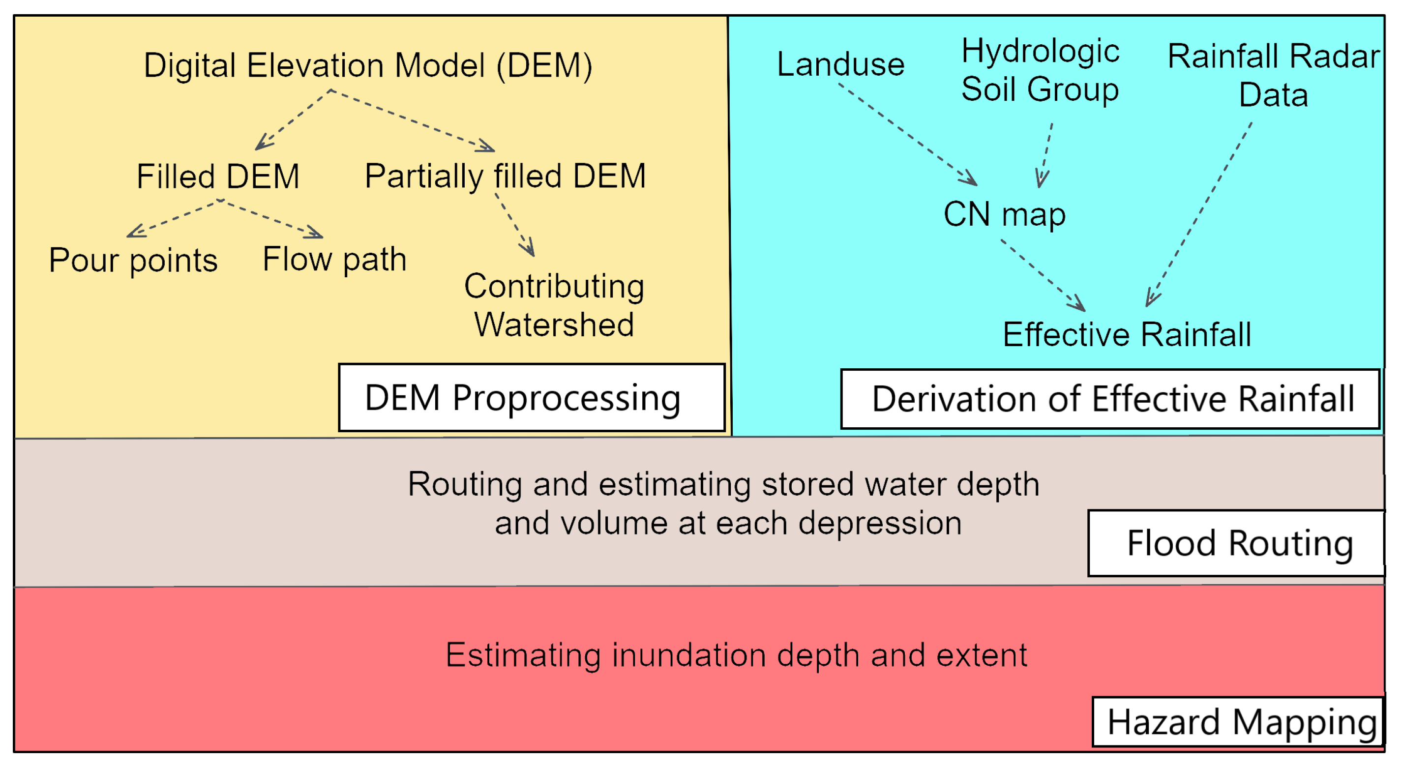
We implemented three main steps to estimate the inundation depth, extent, and volume in a study area, as shown in Figure 3: (1) DEM prepossessing and derivation of effective rainfall, (2) flood routing and (3) hazard mapping.
- 1
- DEM prepossessing and derivation of effective rainfall: The first step in delineating a watershed is to fill sinks, in which existing depressions (called also sinks and pits) in the DEM are filled to guarantee stream connectivity. However, excess runoff is accumulated in these depressions in urban watersheds. Therefore, it is vital to identify them in urban areas as they are more prone to urban flooding. Depressions were identified by computing the elevation difference between the filled DEM and the original DEM in ArcGIS (v. 10.5.1). After that, only depressions with a depth of more than 0.20 m (the vertical accuracy of the original DEM) and surface areas bigger than 1000 m2 were considered. We calculated the flow direction and the flow accumulation using the D8 algorithm from the filled DEM and used them to estimate the flow paths, spilling points, and the vertical hierarchy of the depressions. Finally, we obtained the partially filled DEM by filling the depressions in the original DEM except for the selected depressions. The partially filled DEM was used to estimate the contributing watershed for each depression. The curve number method was used to estimate the effective rainfall for each pixel. Therefore, the curve number map for Berlin was created based on the soil type, hydrologic condition from [29] and land use from an open street map [30], Figure 3 shows the implemented workflow.
- 2
- Flood routing: In general, rainfall is transformed to either evapotranspiration, infiltration, or surface and sewer system runoff. Runoff at the surface and in the urban storm drainage system could contribute to pluvial flooding in terms of inundation of areas in depressions. This study neglected the latter because of the difficulties of obtaining the detailed urban storm drainage system data if they exist. In addition, the urban storm drainage system tends to be ineffective in the case of intensive rainstorms [41,42]. Using the Hydrologic Engineering Center—Hydrologic Modeling System (HEC-HMS) model [43], we estimated the excess runoff based on the SCS method [44] for precipitation depths ranging from 30 to 150 mm (10 mm increments), performed the runoff routing, and estimated the stored depth and volume at each depression.
- 3
- Hazard mapping: We estimated the water depth and inundation extent inside the depressions by subtracting the obtained water level minus the elevation for each pixel from the original DEM in ArcGIS (v. 10.5.1).
3.3. TWI Method
The TWI was initially introduced by [45] for conceptual hydrological modeling at the catchment scale on mountainous and hilly terrain. It was intended to reflect the tendency of a location along a hillslope to generate surface runoff from saturation excess but was later used to generally represent the tendency of a location to accumulate water subject to the local slope and the upstream contributing area. To that end, it was also suggested as an index for pluvial flooding in urban areas [23]. We obtained the TWI from a DEM using ArcGIS (v. 10.5.1): the eight-direction (D8) flow model was used to calculate the flow direction from the fully filled DEM, upslope area and local slope. Finally, we estimated the TWI on a cell-by-cell basis, as shown in Figure 1b:
The parameter a represents the upslope contributing area per grid length, and is the local slope angle.
We applied the TWI method in Berlin to identify flood-prone areas (referred to as FP). The underlying assumption is that a location is flood-prone if its TWI exceeds a certain threshold . The estimation of employs the maximum likelihood method, as described in detail by [25,26,27]. We used the inundation maps from the TELEMAC-2D model for two case studies within Berlin, which have frequent flooding, to estimate the TWI threshold () for each case independently.
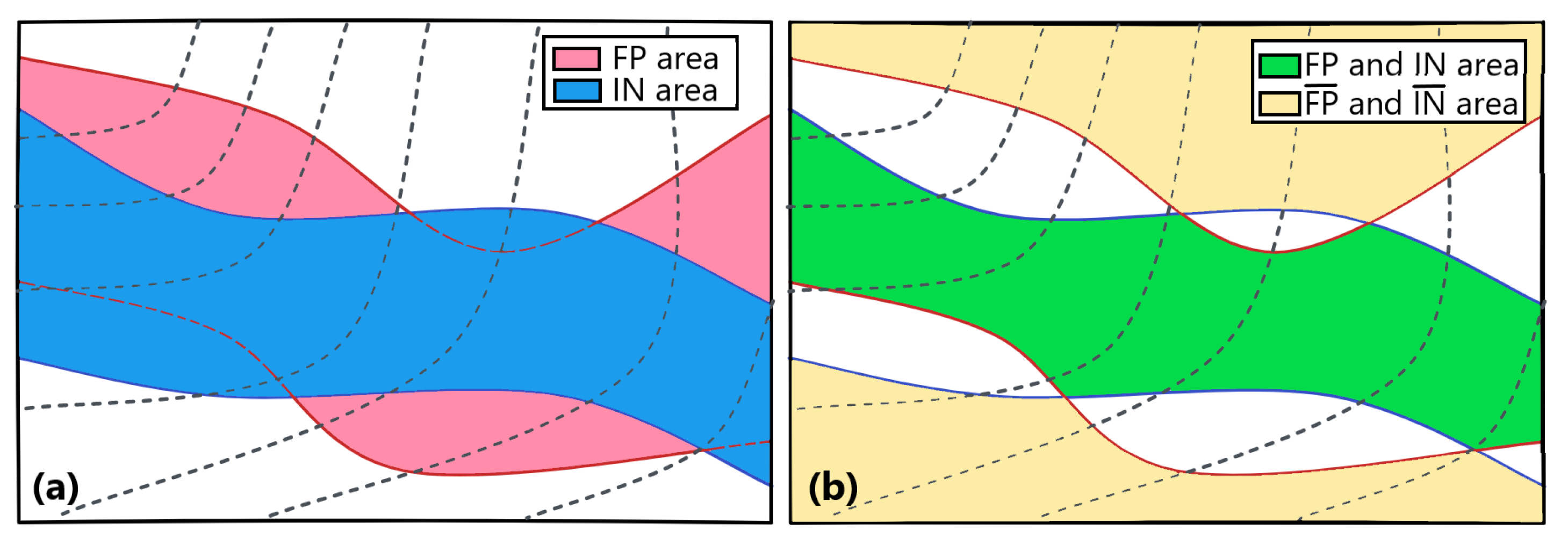
Hence, FP represents the pluvial flood-prone area that meets the condition TWI > , and IN represents the inundated area as obtained from the TELEMAC-2D model for a certain precipitation event depth (simulated water depth h is larger than 0, ) as shown in Figure 4a. The probability of correctly identifying the flood-prone area, or the likelihood function for (L(|W)), can be calculated for various values of as follows:
where indicates the probability that a certain pixel within a spatial window W is identified both as inundated (based on the calculated inundation maps from TELEMAC-2D model) and (based on the TWI method), and conditioned on a given value of . Furthermore, indicates the probability that a certain pixel within the spatial window W is neither identified as nor as conditioned on a given .
and could be expanded by utilizing the product rule of the probability theory [46], as follows:
where and indicate the probability that a certain pixel within the spatial window W is and , respectively, conditioned on a given value of . The indicates the probability that a certain pixel within the spatial window W is identified as on the condition that it is , and indicates the probability that a certain pixel within the spatial window W is identified as on the condition that it is , for a given value of .
Maximum Likelihood Estimation
- 1
- Mesoscale estimations: The terrain in Berlin is relatively flat. Therefore, we calculated the using the spatial extent of the case study area as follows:where indicates the area within the case study area (area with TWI values > ) and is the case study area.
- 2
- Microscale estimations: and were calculated using the spatial extent of the selected window within the study area, as shown in Figure 5 as follows:where indicates the area that is defined as both and within the selected window (the green-colored area in Figure 4b), and indicates the area that is defined as within the selected window. Furthermore, indicates the area that is defined as neither nor within the selected window (the yellow-colored area in Figure 4b) and indicates the area that is defined as within the selected window.
Finally, we calculated the likelihood function Equation (2) and estimated the TWI threshold value () as the value that maximizes the likelihood function.
3.4. Benchmarking Experiments
1—Case Studies
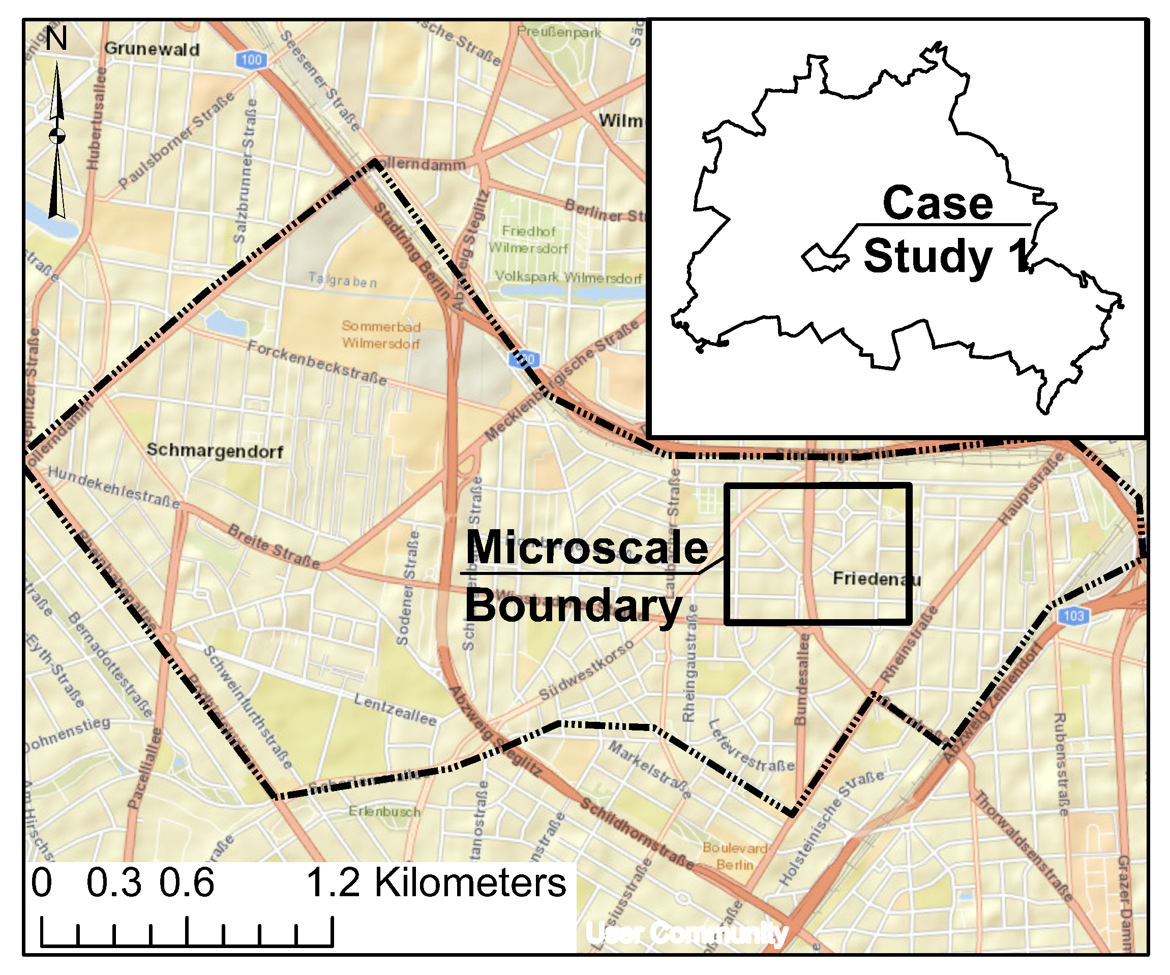
We selected two case studies within Berlin, as shown in Figure 1a. They have been frequently inundated in the last decades [47]. Case study 1 and 2 areas are 6.3 and 12.5 km2, respectively. Depressions represent 14% and 8% of case study 1 and 2 areas, respectively. Depressions with a surface area more than 1000 m2 represent approximately 89% of the area of the total depression in the two case studies. The estimated historical precipitation depth that caused flooding in the period between 2005 and 2019 for the two case studies ranges from 30 to 150 mm based on the rainfall radar data analysis [31,32].
2—Evaluation Metrics
We compared the output of the two methods, FSM and TWI, with the output from the TELEMAC-2D model and considered the latter as a true reference. Considering the uncertainty of the FSM method, TWI method, and TELEMAC-2D model and the difference in the computational domain discretization (i.e., pixel-based for FSM method and TWI method, and unstructured triangular mesh for TELEMAC-2D model), we considered pixels with a simulated water depth (h) higher than 0.10 m as flooded for both the FSM method and the TWI method for comparing and evaluating the performance of the two methods. Then, we categorized every pixel into one of the following four categories:
- 1
- True positive (TP): correctly classified as flooded;
- 2
- True Negative (TN): correctly classified as non-flooded;
- 3
- False positive (FP): incorrectly classified as flooded;
- 4
- False negative (FN): incorrectly classified as non-flooded.
The performance of the applied methods was then evaluated based on the following metrics (Table 1):
The Sensitivity (TPR) refers to the proportion of the pixels that correctly identified as inundated among all the inundated pixels from the true reference. The Matthews correlation coefficient (MCC) measures the correlation between binary classifications, and the Flood Area Index (FAI) refers to the agreement in identifying the inundated area with the true reference.
We evaluated the output water depth (h) from the FSM method and TELEMAC-2D model by the Nash Sutcliffe Efficiency index (NSE) [48].
where is the water depth from the TELEMAC-2D model; is the water depth from the FSM method; is the mean water depth from TELEMAC-2D model, and n is the total number of pixels. NSE value is between and 1.0, values less than or equal to zero indicate unacceptable performance, a value between 0 and 1.0 indicates acceptable performance and 1.0 indicates total agreement.
4. Results and Discussion
We applied the FSM and TWI methods to identify pluvial flood prone areas for two case studies in Berlin by using input precipitation depths from 30 to 150 mm (10 mm increments) and compared the results to the inundation extent obtained from the TELEMAC-2D model. We structured the result section as follows: First, we estimated the TWI threshold () for the two case studies separately, considering IN areas as areas with water depths (h) greater than zero (h > 0). We then estimated the TWI threshold () for various definitions of IN areas (water depth (h) greater than zero, 1, 5, and 10 cm) for case study 1. Finally, we evaluated the performance of the FSM method and the TWI method compared to the TELEMAC-2D model performance.
4.1. Maximum Likelihood Estimation
We calculated the likelihood function for all possible values of by using Equation (2). This was performed separately for different event precipitation depths between 30 and 150 mm. Figure 6 shows the estimated maximum likelihood for a 100 mm precipitation depth for case study region 1. The TWI threshold () value associated with the maximum likelihood is = 5.3. This means, hence, that for a 100 mm storm, we would expect all areas in region 1 with a to inundate. Furthermore, we defined the maximum likelihood interval as the interval that represents the 99th percentile of the estimated maximum likelihood values. The maximum likelihood interval is [4.8, 6.4] for case study 1 for the 100 mm precipitation depth, as shown in Figure 6.
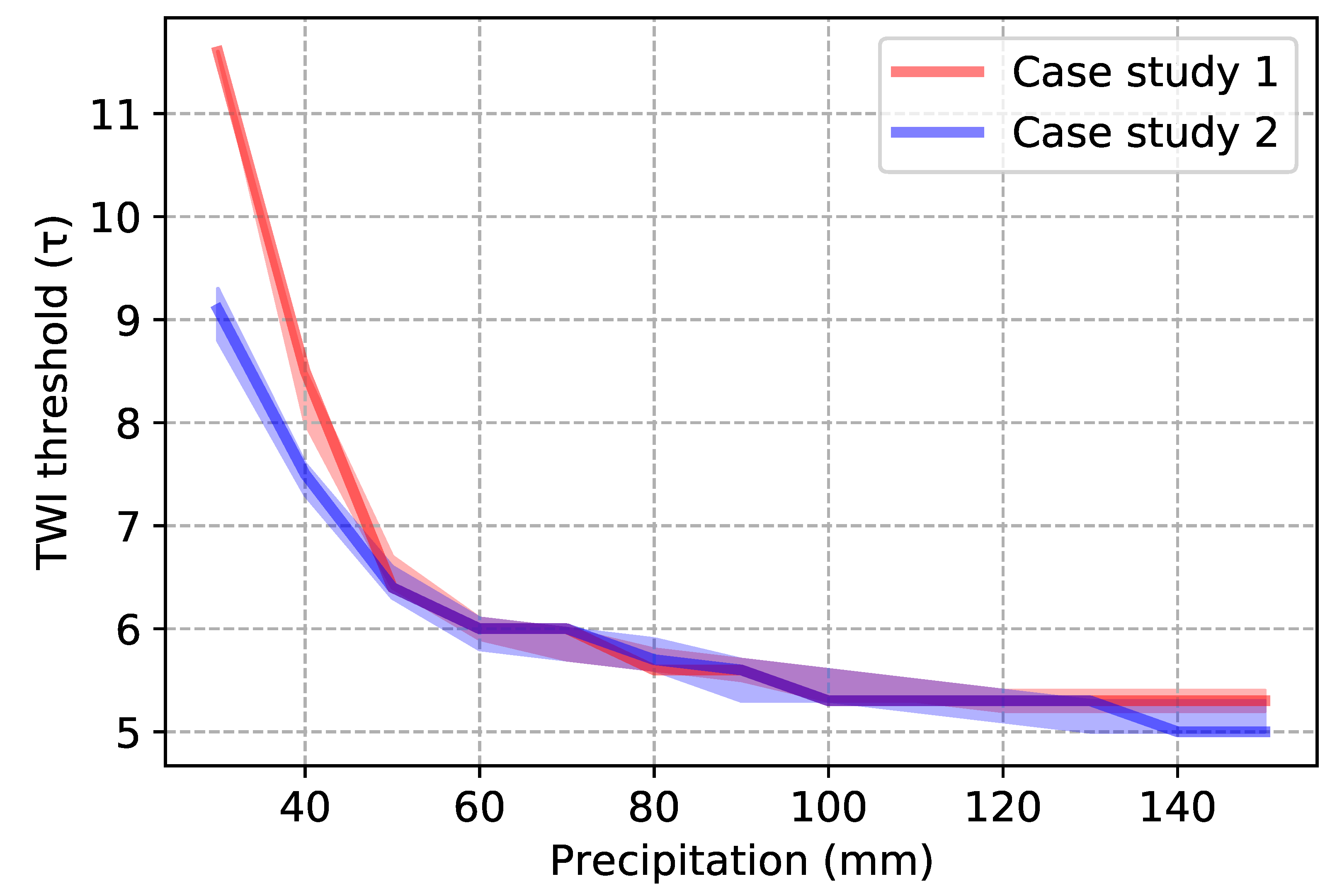
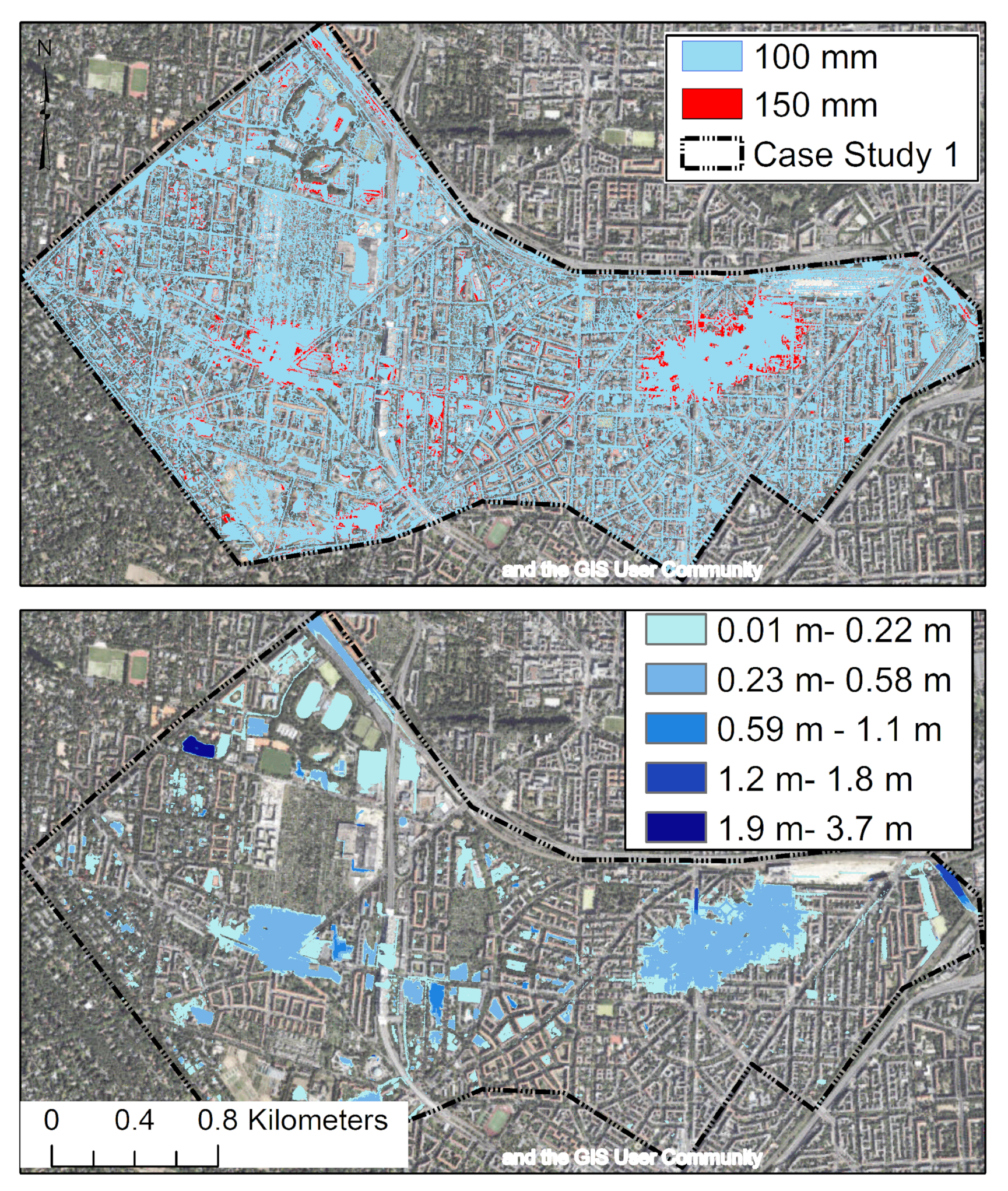
Figure 7 shows the estimated TWI threshold () for the two case studies together with the 99% confidence interval, depending on precipitation depth. The values of are very similar for the two case studies. It also appears that after exceeding a certain precipitation threshold (100 mm in the two case studies), does not decrease much more with increasing the precipitation. A possible explanation is that a further increase in precipitation does not increase the inundation extent but only the inundation depth. This is shown in Figure 8 with the inundation-extent for 100 and 150 mm precipitation depths and the inundation depth difference from the two precipitation depth scenarios.
4.2. Water Depth (h) Threshold
References [25,26,27] defined inundated areas as areas with a water depth greater than zero. However, inundation starts to become a disturbance for pedestrians when the water depth exceeds 10 cm (height of sidewalk) and cars when the water depth is typically higher than 30 cm (depth at which the floodwater reaches the car electronics and causes traffic chaos) [24]. Therefore, we estimated the TWI threshold () by defining the inundated areas as areas with water depths greater than zero, 1, 5, and 10 cm for case study 1. The likelihood function for case study 1 for a precipitation depth 100 mm is shown in Figure 9 for the different water depth thresholds as a function of . As expected, the value corresponding to the maximum likelihood increased with increasing the water depth threshold. As a consequence, flood-prone areas as identified by the TWI method decrease with an increasing water depth threshold, as shown in Figure 10. Furthermore, Figure 10 shows that estimated flood-prone areas did not change with increasing the water depth threshold from 1 to 10 cm, which could be explained by the low difference between the estimated TWI thresholds () for these water depth thresholds.
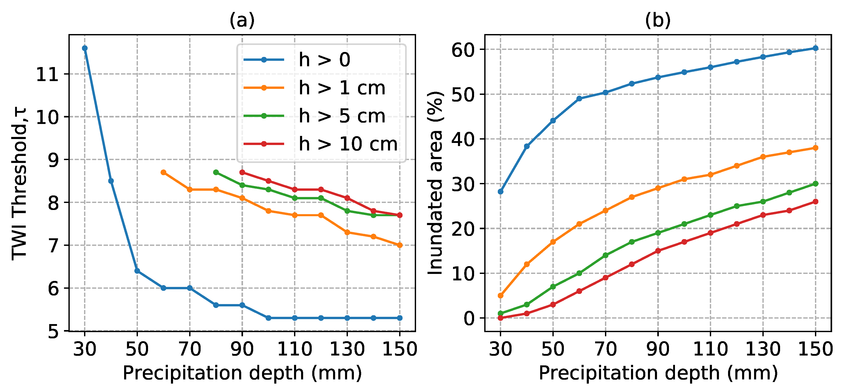
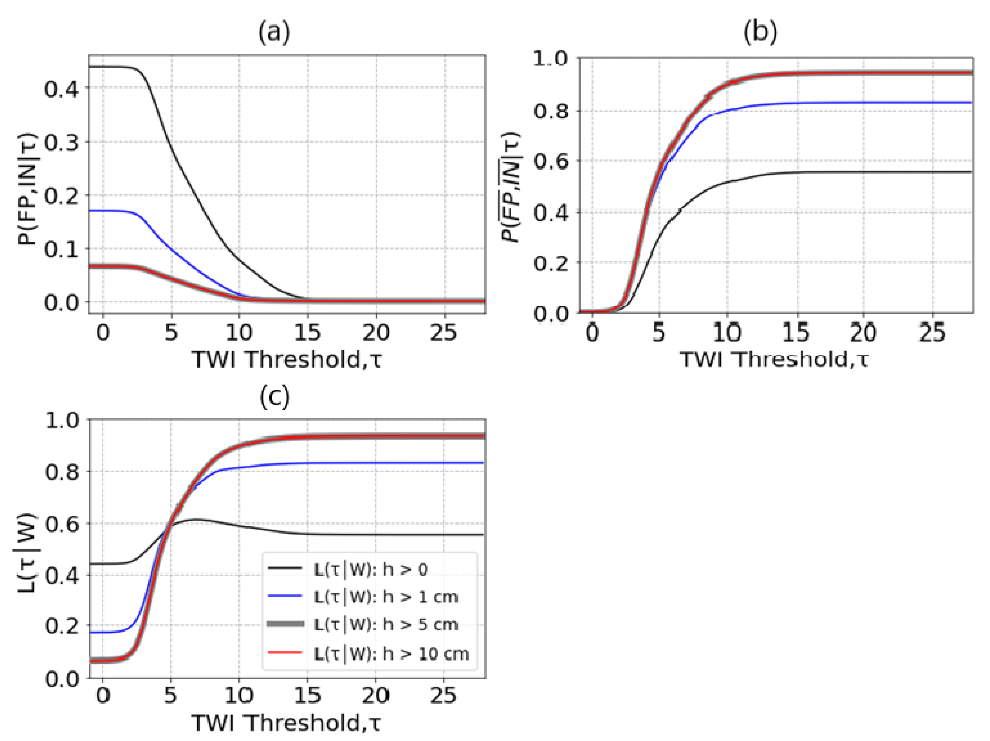
Figure 11a shows the estimated TWI threshold () for different water depths thresholds and precipitation depths for case study 1. As we can see, the TWI method could not find a local maximum for the likelihood function and hence no value for lower precipitation depths together with water depth thresholds greater than zero (h > 0). Obviously, this limits the applicability of the TWI method to identify flood-prone areas for impact-relevant water depth thresholds in combination with rather low (but also impact-relevant) precipitation scenarios. The reason behind the inability to identify a value for in such cases (i.e., the inability to find a local maximum in the likelihood function) can be explained by looking at the two components of the likelihood function Equation (2): the (the probability of areas being identified both as flood-prone by the TWI method and as inundated based on the TELEMAC-2D model), and (the probability of areas being neither identified as flood-prone nor modeled as inundated). As we can see in Figure 12a, an increase in the water depth threshold (h) beyond 0 cm reduces the inundated area (IN) so much that the probability term is reduced to just a negligible contribution to the maximum likelihood value . As a consequence, is dominated by the probability of identifying an area as neither flood-prone nor inundated (), as shown in Figure 12b,c. In that case, maximizing corresponds to choosing the maximum possible TWI value in the spatial domain W.
4.3. Evaluating FSM and TWI Methods Performance
Figure 13 shows the performance of the FSM and TWI methods with regards to their ability to represent the inundation extent as simulated by the TELEMAC-2D model for the different precipitation scenarios (from 30 to 150 mm) and case study areas. A pixel is considered as flooded if the simulated water depth (h) exceeds 0.10 m. For this threshold of h, the performance of the TWI method could only be measured for precipitation depths of 90 mm and more (see the above discussion about how the estimation of is limited).
Figure 13 highlights two main results: first, the FSM method clearly outperforms the TWI method for those precipitation depths for which both methods are applicable (i.e., 90 mm and more). This holds for both case studies and all performance metrics (sensitivity TPR, Matthew Correlation Coefficient MCC, Flood Area Index FAI). For a 100 mm precipitation event, e.g., the FSM method has a TPR of 0.72 and 0.68 (case studies 1 and 2) while the TWI method only achieves TPR values of 0.37 and 0.26 for the same event.
Second, the performance of all methods tends to increase with precipitation depth. This is most pronounced for case study 1 with both methods across all performance metrics: TPR increases from 0.31 to 0.79, MCC from 0.08 to 0.76, and FAI from 0.02 to 0.67. For case study 2, the performance metrics increase steeply at first. Then, MCC and FAI values of the FSM method slightly decline at precipitation depths of more than 110 mm, and TPR exhibits a more pronounced decrease beyond 100 mm of precipitation. The reason for this behavior of the FSM method in case study 2 is that the depressions in this area were completely filled with excess runoff at a precipitation depth around 100 m, so that inundation spread to areas outside the depressions. The FSM method, however, only represents inundation within depressions. Therefore, the method fails to represent flooding beyond depressions and hence shows a performance decrease for such situations. For the TWI method, such a decrease in performance does not occur as it is not explicitly limited to represent depressions (but obviously, the performance of the TWI method continues to increase at a much lower performance level). Please note that, for a more comprehensive evaluation, we provided additional evaluation metrics (precision, specificity, accuracy, and balanced accuracy) in Figure S1, Figure S1 in the supplementary material. However, these additional metrics do not provide new insights as to the differences in performance for the different models, case studies, and precipitation thresholds, so we do not discuss them here in further detail.
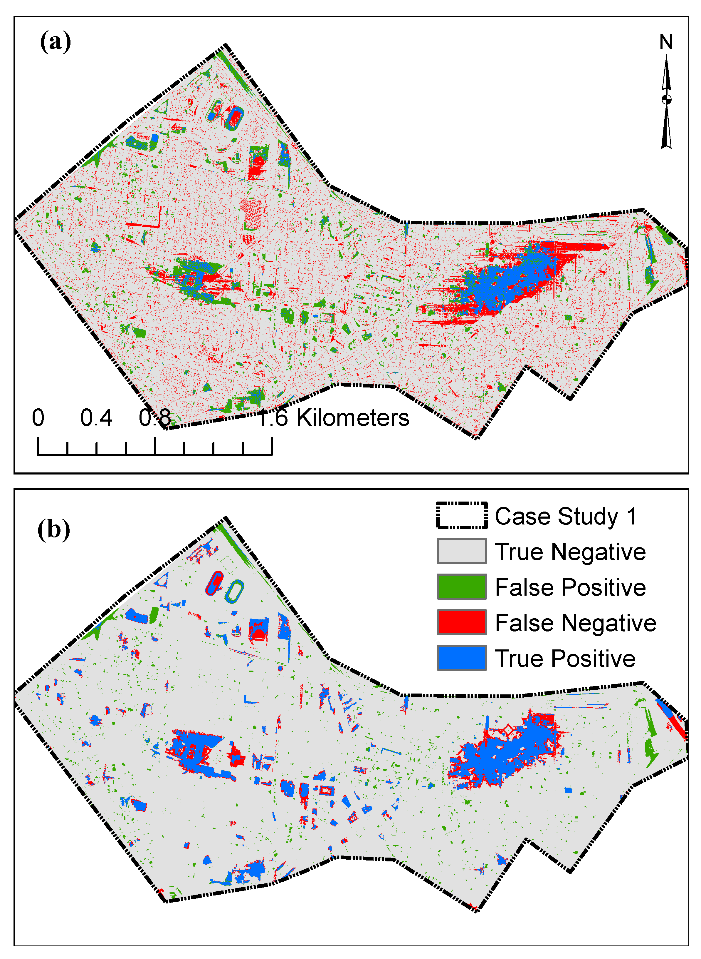
In Figure 14, we compare the spatial distribution of inundated areas from FSM and TWI methods with the inundation obtained from the TELEMAC-2D model for a 100 mm precipitation depth scenario. With this figure, we can better understand why the FSM method outperforms the TWI method so clearly. Obviously, the TWI method fails to identify the inundated areas since the TWI concept does not include the concept of a “depression” as a flood-prone structure and hence fails to correctly detect depressions in terms of flood-prone areas. It is exactly the inherent strength of the FSM method to identify such depressions, so that the inundation extent obtained from the FSM method agrees well with the TELEMAC-2D model.
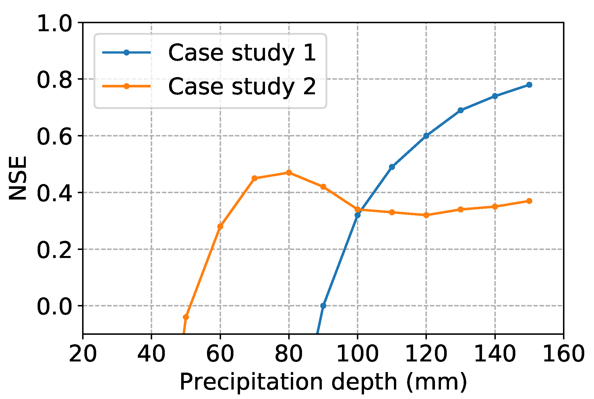
In order to evaluate the ability of the FSM method not only to identify flood-prone areas but also the water depth in inundated areas, we calculated the Nash–Sutcliffe Efficiency (NSE) for the two case studies, as shown in Figure 15. The NSE values for case study 1 continuously increase with precipitation depth from −68.66 to 0.78. For case study 2, the NSE increases from −4.42 to 0.47, and starts to saturate (and slightly decrease) at precipitation depths above 70 mm. Given that the NSE indicates skill only for values above 0 (as compared to just assuming an average observation), the FSM method can be considered as skillful to quantify inundation depth only for precipitation depths beyond 90 (case study 1) and 50 mm (case study 2).
5. Conclusions
Loss and damage caused by pluvial floods are increasing globally, yet the establishment of accurate hazard and risk maps is still impeded by high computational costs and the resource-intensive model setup of hydrodynamic models. At the same time, the availability of high-resolution DEMs is increasing, which means that limitations in terms of the availability of high-quality data are not as acute as, e.g., a decade ago. Still, we require effective and efficient techniques to capitalize on the potential of these data. In the present study, we evaluated two methods that have been suggested in the recent literature to identify urban areas that are prone to pluvial flooding, namely the Fill–Spill–Merge (FSM) method and the Topographic Wetness Index (TWI) method. As a reference for this evaluation, we used the hydrodynamic model TELEMAC-2D. As case studies for this evaluation, we selected two areas in the city of Berlin, Germany.
The TWI method has the obvious advantage that a map of TWI values can be created with minimal effort from a DEM. The TWI method, however, requires a “calibration” in the sense that a TWI threshold has to be estimated above which a location is considered as flood-prone (by using maximum likelihood estimation). This calibration has to be repeated for each precipitation depth of interest. To this end, a reference is required, here the simulation results of a hydrodynamic model (TELEMAC-2D). While this requirement is certainly undesirable, as it again involves the effort to set up and apply a hydrodynamic model, we found that the identified values of were similar for the two case study areas, so that there might be potential to transfer threshold values between regions of application. Unfortunately, though, we found serious limitations in the applicability of the TWI method, at least in a rather flat terrain such as Berlin. Using maximum likelihood estimation, we were unable to identify a local likelihood maximum and hence a value for for lower but still impact-relevant precipitation depths. We were only able to estimate across the entire range of precipitation event depths from 30 to 150 mm in the case we defined an “inundated area” as an area where the water depth exceeded 0 m. However, if we defined inundation as a water depth exceeding 0.1 m, we were only able to identify for precipitation depths of 90 mm and more.
Apart from this serious limitation, the FSM method clearly outperformed the TWI method when it came to detecting flood-prone areas in terms of inundation above 0.1 m. This superiority of the FSM method held for both case study regions and across all considered performance metrics (sensitivity TPR, Matthew Correlation MCC, Flood Area index FAI). The main reason for the failure of the TWI method was that inundation patterns in urban areas are dominated by depressions, while the TWI method has no “notion” of depressions as a structural element that is specifically prone to the accumulation of excess runoff.
While the FSM method was clearly superior to the TWI method, we also found that its performance tends to be higher with increasing event precipitation. For case study 2, however, we also found that the performance of the FSM method can start to decline with very high precipitation depths in case inundation starts to spread beyond depression structures. While the FSM method is theoretically able to point out flood-prone areas and quantify the water depth in flooded areas, this ability was only recognizable beyond minimum precipitation depths of 50 and 90 mm (case study 2 and 1, respectively).
In summary, however, our study showed that at least for the investigated case study areas, the simple and easy to apply TWI method cannot at all compete with the FSM method. Another large advantage of the FSM method is that it does not need to be calibrated to the output of a hydrodynamic model, while its application is about 600 times faster than the hydrodynamic model. Therefore, while the transferability of the FSM method appears high, it is still limited by the effort to actually set up the required model chain: this requires the DEM pre-processing and depression analysis as well as the implementation of runoff routing in a hydrological model. Prospective research should hence aim at providing more efficient and reproducible software tools so that future efforts can advance with more informative and extensive benchmarking experiments.
Supplementary Materials
The following are available online at https://www.mdpi.com/article/10.3390/w13182476/s1, Figure S1: Performance indices for the FSM and TWI methods for different precipitation scenarios.
Author Contributions
Conceptualization, O.S. and M.H.; methodology, software, formal analysis, O.S.; writing—original draft preparation, O.S. and M.H.; visualization, O.S. and M.H.; supervision, A.B. and M.H.; project administration, O.S. and A.B.; funding acquisition, O.S. and A.B. All authors have read and agreed to the published version of the manuscript.
Funding
This research was funded by the Deutscher Akademischer Austauschdienst (DAAD).We acknowledge the support of the Deutsche Forschungsgemeinschaft and Open Access Publishing Fund of the University of Potsdam.
Conflicts of Interest
The authors declare no conflict of interest.
References
- Smith, M.B. Comment on ‘Analysis and modeling of flooding in urban drainage systems’. J. Hydrol. 2006, 317, 355–363. [Google Scholar] [CrossRef]
- Nofal, O.M.; Van De Lindt, J.W. Understanding flood risk in the context of community resilience modeling for the built environment: Research needs and trends. Sustain. Resilient Infrastruct. 2020, 1–17. [Google Scholar] [CrossRef]
- Tabari, H.; Asr, N.M.; Willems, P. Developing a framework for attribution analysis of urban pluvial flooding to human-induced climate impacts. J. Hydrol. 2021, 598, 126352. [Google Scholar] [CrossRef]
- Bronstert, A.; Agarwal, A.; Boessenkool, B.; Crisologo, I.; Fischer, M.; Heistermann, M.; Köhn-Reich, L.; López-Tarazón, J.A.; Moran, T.; Ozturk, U.; et al. Forensic hydro-meteorological analysis of an extreme flash flood: The 2016-05-29 event in Braunsbach, SW Germany. Sci. Total Environ. 2018, 630, 977–991. [Google Scholar] [CrossRef] [PubMed]
- Maksimović, Č.; Prodanović, D.; Boonya-Aroonnet, S.; Leitão, J.P.; Djordjević, S.; Allitt, R. Overland flow and pathway analysis for modelling of urban pluvial flooding. J. Hydraul. Res. 2009, 47, 512–523. [Google Scholar] [CrossRef]
- Guerreiro, S.B.; Glenis, V.; Dawson, R.J.; Kilsby, C. Pluvial flooding in European cities—A continental approach to urban flood modelling. Water 2017, 9, 296. [Google Scholar] [CrossRef] [Green Version]
- Schanze, J. Pluvial Flood Risk Management: An Evolving and Specific Field. J. Flood Risk Manag. 2018, 11, 227–229. [Google Scholar] [CrossRef]
- Di Salvo, C.; Ciotoli, G.; Pennica, F.; Cavinato, G.P. Pluvial flood hazard in the city of Rome (Italy). J. Maps 2017, 13, 545–553. [Google Scholar] [CrossRef] [Green Version]
- Leal, M.; Boavida-Portugal, I.; Fragoso, M.; Ramos, C. How much does an extreme rainfall event cost? Material damage and relationships between insurance, rainfall, land cover and urban flooding. Hydrol. Sci. J. 2019, 64, 673–689. [Google Scholar] [CrossRef]
- Kumar, S.; Agarwal, A.; Villuri, V.G.K.; Pasupuleti, S.; Kumar, D.; Kaushal, D.R.; Gosain, A.K.; Bronstert, A.; Sivakumar, B. Constructed wetland management in urban catchments for mitigating floods. Stoch. Environ. Res. Risk Assess. 2021, 1–20. [Google Scholar] [CrossRef]
- Nofal, O.M.; van de Lindt, J.W. Probabilistic flood loss assessment at the community scale: Case study of 2016 flooding in Lumberton, North Carolina. ASCE-ASME J. Risk Uncertain. Eng. Syst. Part B Civ. Eng. 2020, 6, 05020001. [Google Scholar] [CrossRef]
- Cauncil, T.E. Directive 2007/60/EC on the assessment and management of flood risks. J. Eur. Union Off. 2017, L288, 27–34. [Google Scholar]
- Zhou, Q.; Mikkelsen, P.S.; Halsnæs, K.; Arnbjerg-Nielsen, K. Framework for economic pluvial flood risk assessment considering climate change effects and adaptation benefits. J. Hydrol. 2012, 414, 539–549. [Google Scholar] [CrossRef]
- Zhang, S.; Pan, B. An urban storm-inundation simulation method based on GIS. J. Hydrol. 2014, 517, 260–268. [Google Scholar] [CrossRef]
- Schumann, G.J.P.; Neal, J.C.; Mason, D.C.; Bates, P.D. The accuracy of sequential aerial photography and SAR data for observing urban flood dynamics, a case study of the UK summer 2007 floods. Remote Sens. Environ. 2011, 115, 2536–2546. [Google Scholar] [CrossRef]
- Neal, J.C.; Bates, P.D.; Fewtrell, T.J.; Hunter, N.M.; Wilson, M.D.; Horritt, M.S. Distributed whole city water level measurements from the Carlisle 2005 urban flood event and comparison with hydraulic model simulations. J. Hydrol. 2009, 368, 42–55. [Google Scholar] [CrossRef]
- Hunter, N.M.; Bates, P.D.; Horritt, M.S.; De Roo, A.; Werner, M.G. Utility of different data types for calibrating flood inundation models within a GLUE framework. Hydrol. Earth Syst. Sci. 2005, 9, 412–430. [Google Scholar] [CrossRef]
- Samela, C.; Persiano, S.; Bagli, S.; Luzzi, V.; Mazzoli, P.; Humer, G.; Reithofer, A.; Essenfelder, A.; Amadio, M.; Mysiak, J.; et al. Safer_RAIN: A DEM-based hierarchical filling-&-Spilling algorithm for pluvial flood hazard assessment and mapping across large urban areas. Water 2020, 12, 1514. [Google Scholar]
- Balstrøm, T.; Crawford, D. Arc-Malstrøm: A 1D hydrologic screening method for stormwater assessments based on geometric networks. Comput. Geosci. 2018, 116, 64–73. [Google Scholar] [CrossRef]
- Manfreda, S.; Samela, C. A digital elevation model based method for a rapid estimation of flood inundation depth. J. Flood Risk Manag. 2019, 12, e12541. [Google Scholar] [CrossRef] [Green Version]
- Samela, C.; Albano, R.; Sole, A.; Manfreda, S. A GIS tool for cost-effective delineation of flood-prone areas. Comput. Environ. Urban Syst. 2018, 70, 43–52. [Google Scholar] [CrossRef]
- Samela, C.; Troy, T.J.; Manfreda, S. Geomorphic classifiers for flood-prone areas delineation for data-scarce environments. Adv. Water Resour. 2017, 102, 13–28. [Google Scholar] [CrossRef]
- Kelleher, C.; McPhillips, L. Exploring the application of topographic indices in urban areas as indicators of pluvial flooding locations. Hydrol. Process. 2020, 34, 780–794. [Google Scholar] [CrossRef]
- Huang, H.; Chen, X.; Wang, X.; Wang, X.; Liu, L. A depression-based index to represent topographic control in urban pluvial flooding. Water 2019, 11, 2115. [Google Scholar] [CrossRef] [Green Version]
- Jalayer, F.; De Risi, R.; De Paola, F.; Giugni, M.; Manfredi, G.; Gasparini, P.; Topa, M.E.; Yonas, N.; Yeshitela, K.; Nebebe, A.; et al. Probabilistic GIS-based method for delineation of urban flooding risk hotspots. Nat. Hazards 2014, 73, 975–1001. [Google Scholar] [CrossRef]
- De Risi, R.; Jalayer, F.; De Paola, F. Meso-scale hazard zoning of potentially flood prone areas. J. Hydrol. 2015, 527, 316–325. [Google Scholar] [CrossRef]
- De Risi, R.; Jalayer, F.; De Paola, F.; Lindley, S. Delineation of flooding risk hotspots based on digital elevation model, calculated and historical flooding extents: The case of Ouagadougou. Stoch. Environ. Res. Risk Assess. 2018, 32, 1545–1559. [Google Scholar] [CrossRef] [Green Version]
- Digitale Geländemodelle—ATKIS DGM. Available online: http://www.stadtentwicklung.berlin.de/geoinformation/landesvermessung/atkis/de/dgm.shtml (accessed on 3 March 2021).
- Ross, C.; Prihodko, L.; Anchang, J.; Kumar, S.; Ji, W.; Hanan, N. HYSOGs250m, global gridded hydrologic soil groups for curve-number-based runoff modeling. Sci. Data 2018, 5, 180091. [Google Scholar] [CrossRef] [PubMed]
- Haklay, M.; Weber, P. Openstreetmap: User-generated street maps. IEEE Pervasive Comput. 2008, 7, 12–18. [Google Scholar] [CrossRef] [Green Version]
- Winterrath, T.; Brendel, C.; Hafer, M.; Junghänel, T.; Klameth, A.; Walawender, E.; Weigl, E.; Becker, A. Erstellung Einer Radargestützten Niederschlagsklimatologie; Freie Universität: Berlin, Germany, 2017. [Google Scholar]
- Kreklow, J.; Tetzlaff, B.; Kuhnt, G.; Burkhard, B. A Rainfall Data Intercomparison Dataset of RADKLIM, RADOLAN, and Rain Gauge Data for Germany. Data 2019, 4, 118. [Google Scholar] [CrossRef] [Green Version]
- Hervouet, J.M. Hydrodynamics of Free Surface Flows: Modelling with the Finite Element Method; John Wiley & Sons: Hoboken, NJ, USA, 2007. [Google Scholar]
- Galland, J.C.; Goutal, N.; Hervouet, J.M. TELEMAC: A new numerical model for solving shallow water equations. Adv. Water Resour. 1991, 14, 138–148. [Google Scholar] [CrossRef]
- Li, Z.; Liu, J.; Mei, C.; Shao, W.; Wang, H.; Yan, D. Comparative Analysis of Building Representations in TELEMAC-2D for Flood Inundation in Idealized Urban Districts. Water 2019, 11, 1840. [Google Scholar] [CrossRef] [Green Version]
- Testa, G.; Zuccalà, D.; Alcrudo, F.; Mulet, J.; Soares-Frazão, S. Flash flood flow experiment in a simplified urban district. J. Hydraul. Res. 2007, 45, 37–44. [Google Scholar] [CrossRef]
- Papaioannou, G.; Efstratiadis, A.; Vasiliades, L.; Loukas, A.; Papalexiou, S.M.; Koukouvinos, A.; Tsoukalas, I.; Kossieris, P. An operational method for flood directive implementation in ungauged urban areas. Hydrology 2018, 5, 24. [Google Scholar] [CrossRef] [Green Version]
- French, R.H.; French, R.H. Open-Channel Hydraulics; McGraw-Hill: New York, NY, USA, 1985. [Google Scholar]
- Blue Kenue™: Software Tool for Hydraulic Modellers. Available online: http://nrc.canada.ca/en/research-development/products-services/software-applications/blue-kenuetm-software-tool-hydraulic-modellers (accessed on 3 March 2021).
- TELEMAC-2D. User Manual of Opensource Software TELEMAC-2D. Report, EDF-R&D. V8P1. 2019. Available online: www.opentelemac.org (accessed on 3 March 2021).
- Di Salvo, C.; Pennica, F.; Ciotoli, G.; Cavinato, G.P. A GIS-based procedure for preliminary mapping of pluvial flood risk at metropolitan scale. Environ. Model. Softw. 2018, 107, 64–84. [Google Scholar] [CrossRef]
- Falconer, R.H.; Cobby, D.; Smyth, P.; Astle, G.; Dent, J.; Golding, B. Pluvial flooding: New approaches in flood warning, mapping and risk management. J. Flood Risk Manag. 2009, 2, 198–208. [Google Scholar] [CrossRef]
- Scharffenberg, W.; Harris, J. Hydrologic engineering center hydrologic modeling system, HEC-HMS: Interior flood modeling. In Proceedings of the World Environmental and Water Resources Congress 2008: Ahupua’A, Honolulu, HI, USA, 12–16 May 2008; pp. 1–3. [Google Scholar]
- Cronshey, R. Urban Hydrology for Small Watersheds; Technical Report; US Dept. of Agriculture, Soil Conservation Service, Engineering Division: Washington, DC, USA, 1986.
- Kirkby, M. Hydrograph Modelling Strategies, 69–90; Peel, R., Chisholm, M., Haggert, P., Eds.; Processes in Physical and Human Geography, Heineman: London, UK, 1975. [Google Scholar]
- Jaynes, E.T. Probability Theory: The Logic of Science; Cambridge University Press: Cambridge, UK, 2003. [Google Scholar]
- Berghäuser, L.; Schoppa, L.; Ulrich, J.; Dillenardt, L.; Jurado, O.E.; Passow, C.; Mohor, G.S.; Seleem, O.; Petrow, T.; Thieken, A.H. Starkregen in Berlin: Meteorologische Ereignisrekonstruktion und Betroffenenbefragung; Universität Potsdam: Brandenburg, Germany, 2021. [Google Scholar]
- Nash, J.E.; Sutcliffe, J.V. River flow forecasting through conceptual models part I—A discussion of principles. J. Hydrol. 1970, 10, 282–290. [Google Scholar] [CrossRef]
Figure 1.
(a) Digital elevation model (DEM) of Berlin, the two case studies and the city districts. (b) The spatial distribution of TWI for Berlin and the city districts.
Figure 1.
(a) Digital elevation model (DEM) of Berlin, the two case studies and the city districts. (b) The spatial distribution of TWI for Berlin and the city districts.
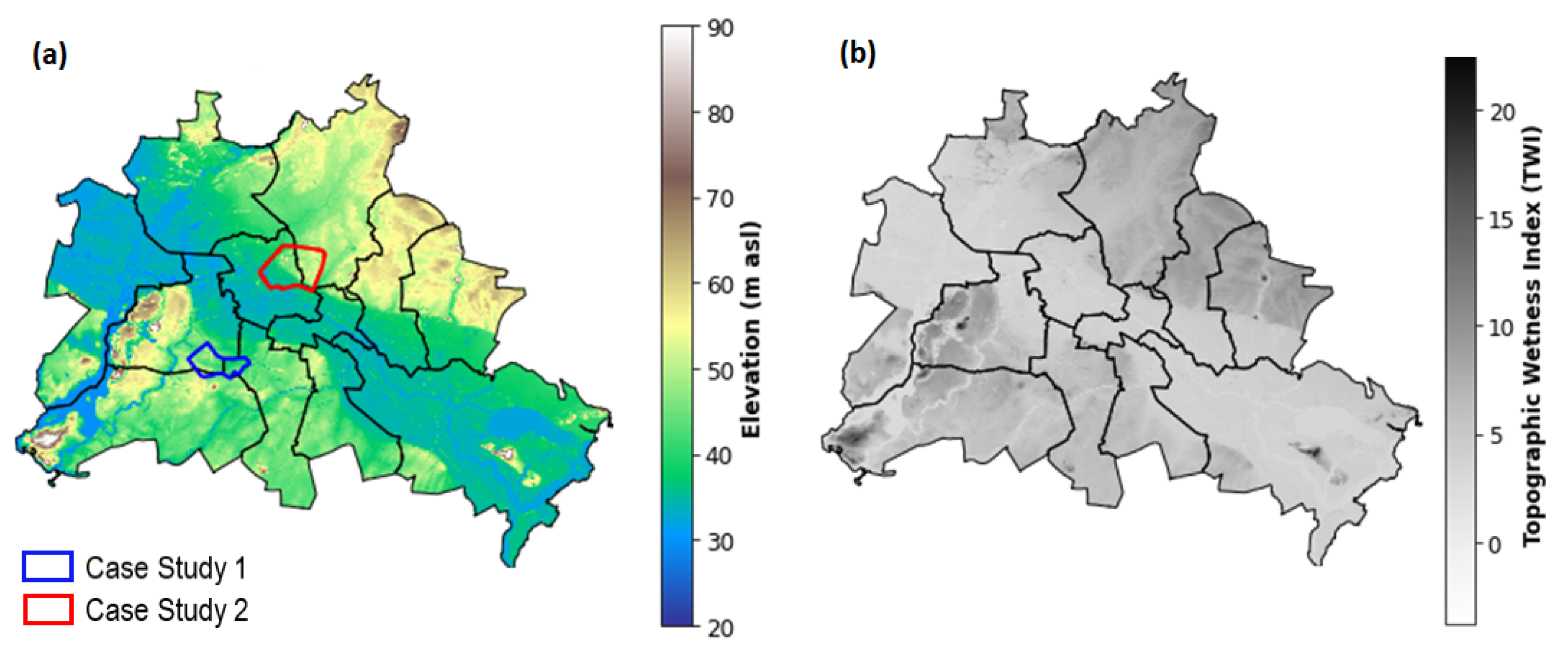
Figure 2.
Process of the FSM method. (a) Runoff flowing process between depressions. (b) Schematic of the nested depressions. (c) Vertical hierarchical tree.
Figure 2.
Process of the FSM method. (a) Runoff flowing process between depressions. (b) Schematic of the nested depressions. (c) Vertical hierarchical tree.
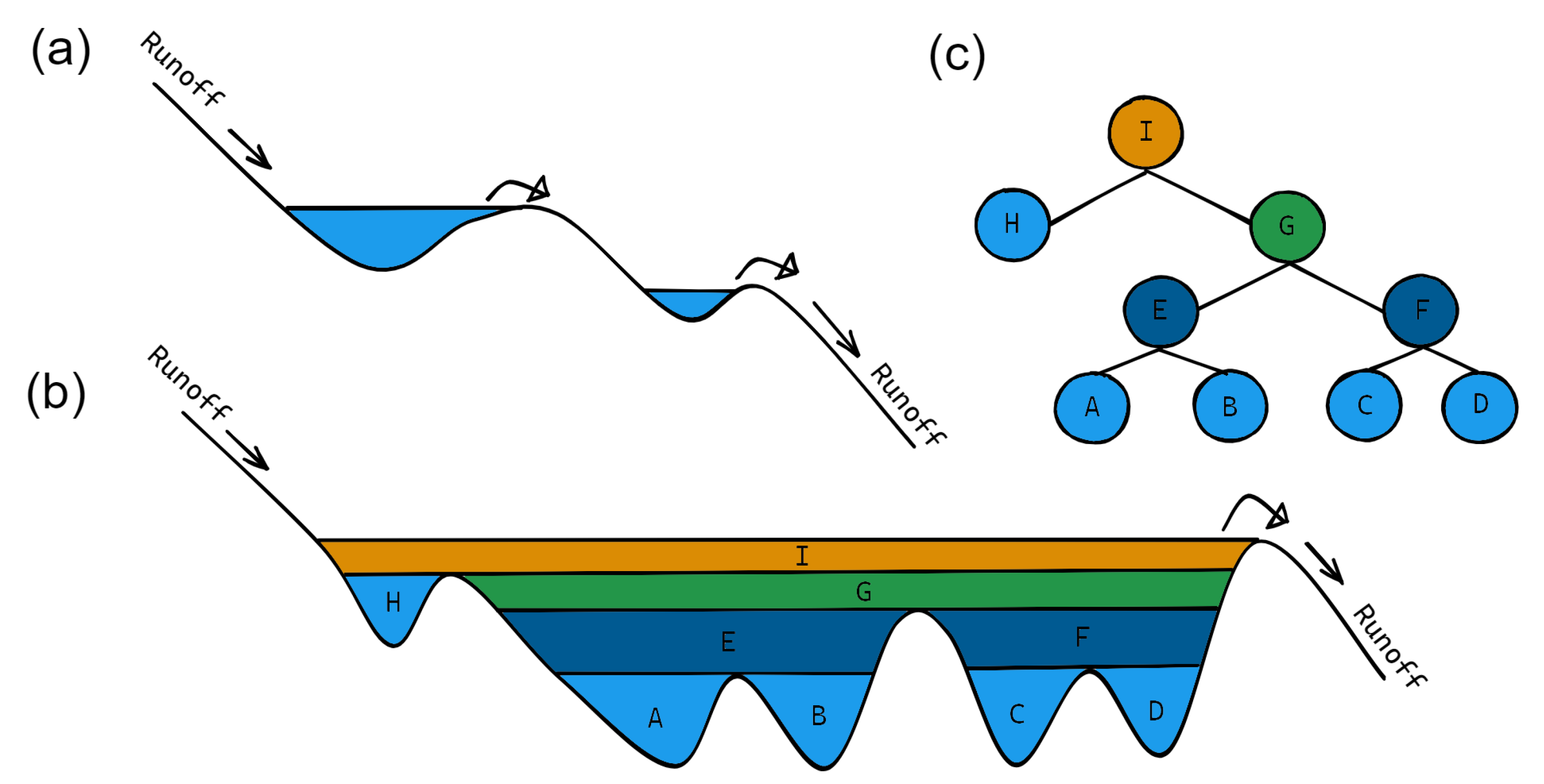
Figure 3.
FSM method’s workflow.

Figure 4.
Flood-prone (FP) and inundated (IN) areas.

Figure 5.
The spatial extent for the mesoscale and microscale.

Figure 6.
Likelihood function L(/W) for a 100 mm precipitation depth (case study 1).
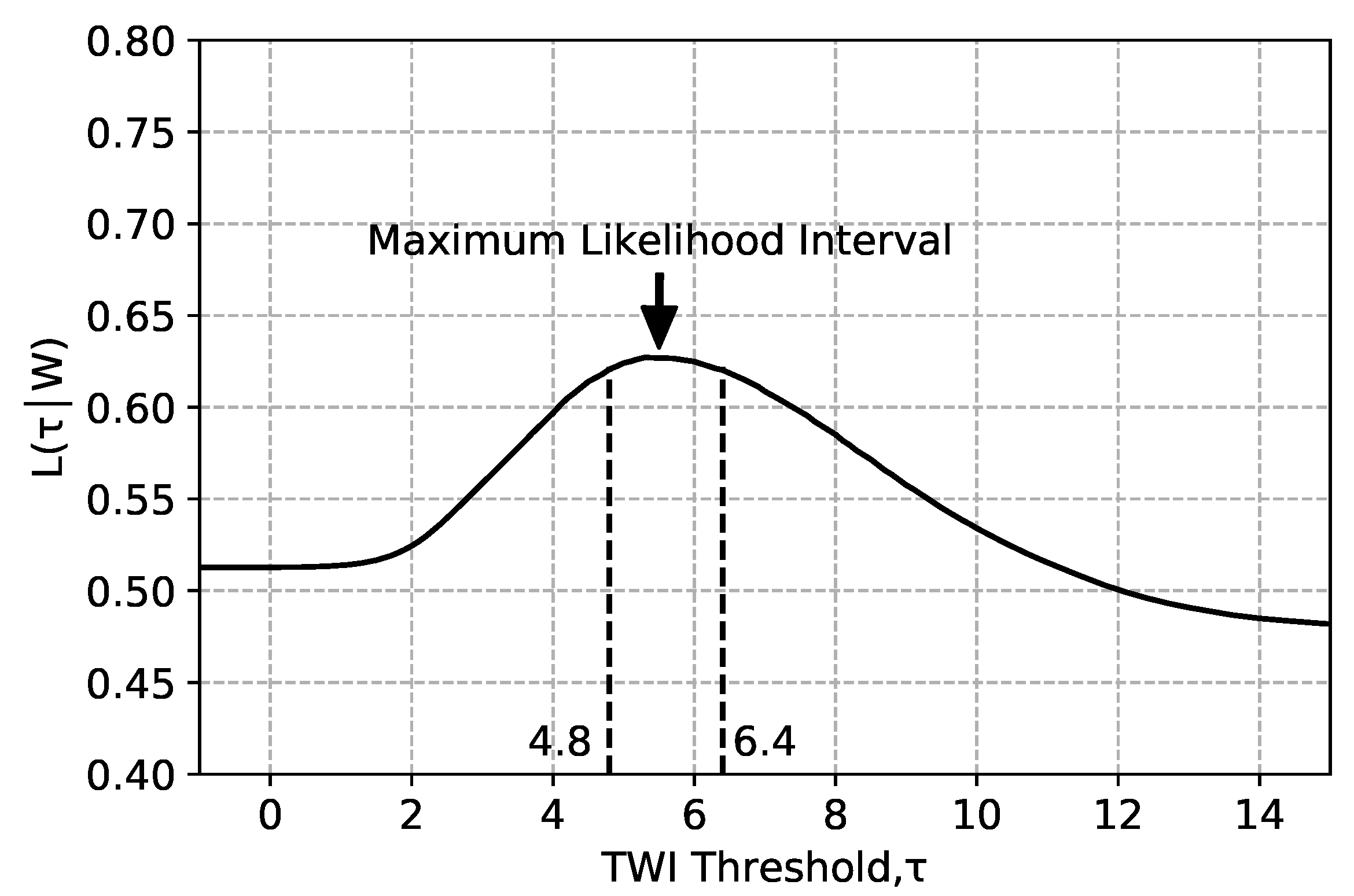
Figure 7.
TWI threshold () for the two case studies with the 99% confidence interval.

Figure 8.
Inundation-extent for 100 and 150 mm precipitation depths for case study 1.

Figure 9.
Likelihood function L(/W) for a 100 mm precipitation depth (case study 1).
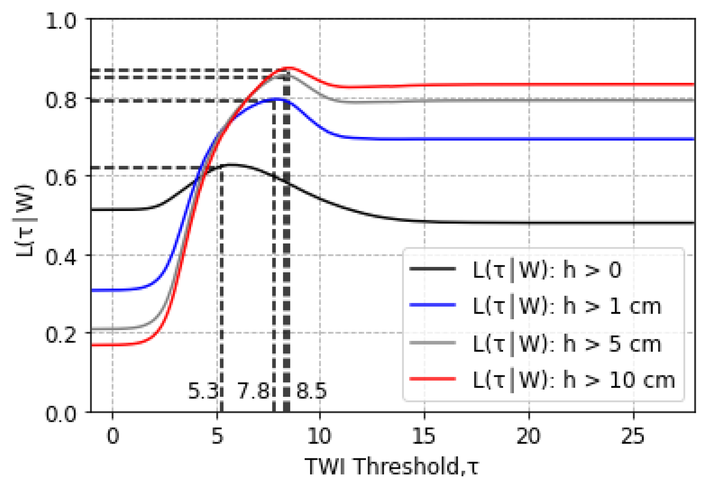
Figure 10.
Flood-prone area (FP) for different water depth thresholds for a 100 mm precipitation depth.
Figure 10.
Flood-prone area (FP) for different water depth thresholds for a 100 mm precipitation depth.

Figure 11.
(a) TWI threshold () for different water depth thresholds (h). (b) Percentage of inundated areas for different water depth thresholds (h).
Figure 11.
(a) TWI threshold () for different water depth thresholds (h). (b) Percentage of inundated areas for different water depth thresholds (h).

Figure 12.
Probabilities of 50 mm precipitation event.

Figure 13.
Performance indices for the FSM and TWI methods for different precipitation scenarios.
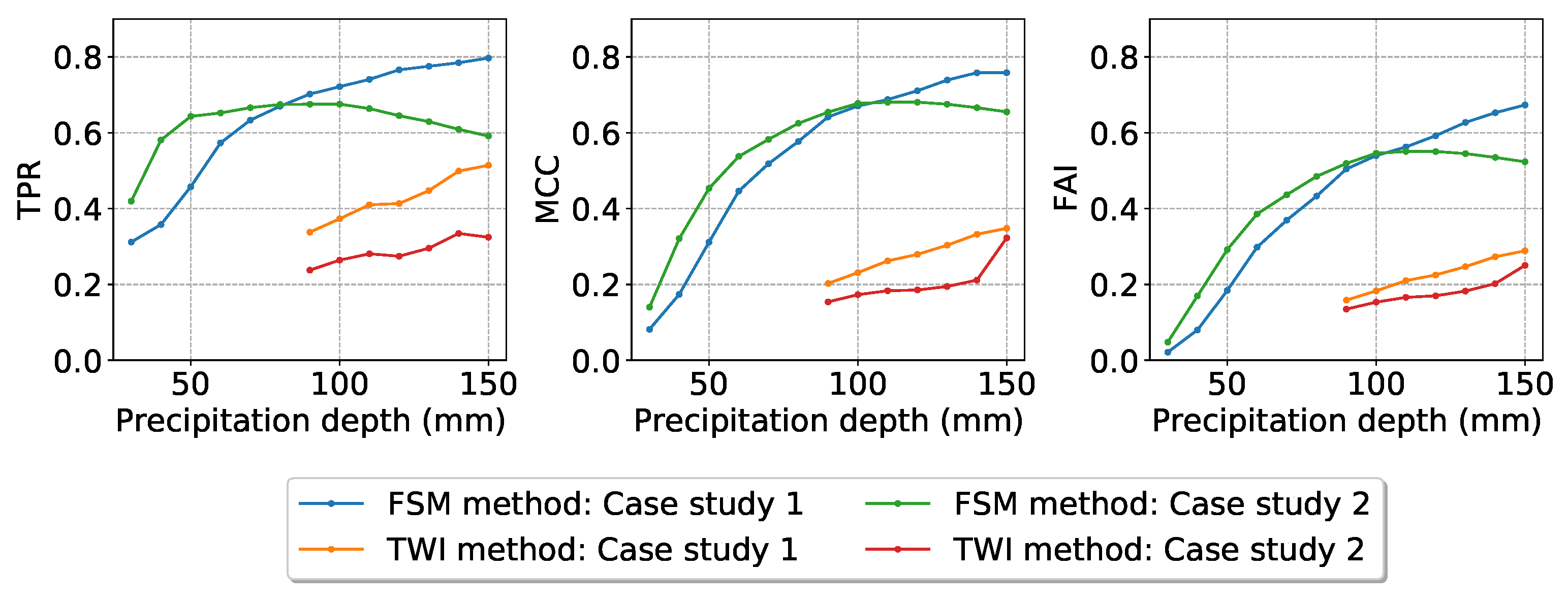
Figure 14.
Comparison of the inundation extent for a 100 mm precipitation event: (a) Comparison of TELEMAC-2D model and the TWI method inundation extents. (b) Comparison of TELEMAC-2D model and the FSM method inundation extents.
Figure 14.
Comparison of the inundation extent for a 100 mm precipitation event: (a) Comparison of TELEMAC-2D model and the TWI method inundation extents. (b) Comparison of TELEMAC-2D model and the FSM method inundation extents.

Figure 15.
NSE values for the simulation results of the two case studies.


Table 1.
Performance indices.
| Index | Equation | Range |
|---|---|---|
| Sensitivity (TPR) | 0 < TPR < 1 | |
| Matthews correlation coefficient (MCC) | −1 < MCC < 1 | |
| Flood Area Index (FAI) | 0 < FAI < 1 |
Publisher’s Note: MDPI stays neutral with regard to jurisdictional claims in published maps and institutional affiliations. |
© 2021 by the authors. Licensee MDPI, Basel, Switzerland. This article is an open access article distributed under the terms and conditions of the Creative Commons Attribution (CC BY) license (https://creativecommons.org/licenses/by/4.0/).
Share and Cite
MDPI and ACS Style
Seleem, O.; Heistermann, M.; Bronstert, A. Efficient Hazard Assessment for Pluvial Floods in Urban Environments: A Benchmarking Case Study for the City of Berlin, Germany. Water 2021, 13, 2476. https://doi.org/10.3390/w13182476
AMA Style
Seleem O, Heistermann M, Bronstert A. Efficient Hazard Assessment for Pluvial Floods in Urban Environments: A Benchmarking Case Study for the City of Berlin, Germany. Water. 2021; 13(18):2476. https://doi.org/10.3390/w13182476
Chicago/Turabian StyleSeleem, Omar, Maik Heistermann, and Axel Bronstert. 2021. "Efficient Hazard Assessment for Pluvial Floods in Urban Environments: A Benchmarking Case Study for the City of Berlin, Germany" Water 13, no. 18: 2476. https://doi.org/10.3390/w13182476
Note that from the first issue of 2016, this journal uses article numbers instead of page numbers. See further details here.