
An Integrated Aquifer Management Approach for Aridification-Affected Agricultural Area, Shengeldy-Kazakhstan


1
Department of Chemical Engineering, The Eastern R&D Center, Ariel University, Ariel 4077625, Israel
2
Institute of Oil and Gas Geology, Satbayev University, Almaty 050013, Kazakhstan
3
Zonal Hydrogeological-Ameliorative Center of the Ministry of Agriculture, Almaty 050018, Kazakhstan
*
Author to whom correspondence should be addressed.
Water 2021, 13(17), 2357; https://doi.org/10.3390/w13172357
Submission received: 24 July 2021
/
Revised: 20 August 2021
/
Accepted: 25 August 2021
/
Published: 27 August 2021
(This article belongs to the Special Issue Climate Smart Irrigation Management for Sustainable Agricultural Cultivation)
Abstract
:Ongoing water-resource depletion is a common trend in southeastern Kazakhstan and in most of Central Asia, making the use of drainage water for freshwater preservation and groundwater recharge a key strategy for sustainable agriculture. Since the Ily River inflow began to decrease, groundwater levels in the Shengeldy study area site have fallen below the drainage pipes. As such, our main research hypothesis was that owing to drainage infiltration, the regional shallow aquifer can be used as an effective additional water source for moistening crop root systems during the irrigation period. The MODFLOW groundwater flow model was used to simulate and quantitatively assess the combined hydrogeological and irrigation conditions of artificial groundwater recharge both from the subsurface drainage and as an additional source for irrigation. The field study showed that the additional groundwater table elevation will reach approximately 1.5 m under the field drainage system and that the additional groundwater recharge influence zone will develop up to 300–350 m from the drains. The MODFLOW simulation together with full-scale experimental studies suggests that under certain conditions drainage water can be applied both as an additional source of irrigation and for aquifer sustainable maintenance.
1. Introduction
In areas where irrigation water is scarce, drainage water reuse can provide benefits by supplementing water resources in parallel applications, enabling drainage volume reduction. A field-test evaluation of the potential of irrigated agriculture expansion through the supplementation of saline drainage waters concluded that new crop and water management strategies and practices should be developed to enable the application of drainage water in agriculture [1]. One such strategy was tested to reduce the water shortage problem in the Middle Euphrates provinces (Iraq) and it indicated that, together with drainage infiltration for reduction, adding brackish water to the summer irrigation enables salinity-sensitive crop cultivation [2]. In the semi-arid Sindh (Indus Delta), drainage allocation for salt-tolerant crops and forest irrigation maintained the salt balance, as salts that were not used by the crop were carried to the groundwater [3]
In a computer-based modeling water-budget approach, the drainage component is important for evaluating groundwater recharge efficiency [4,5]. As such, numerical groundwater models can provide an artificial groundwater recharge assessment [6]. Floodwater harvesting and distribution system techniques for groundwater resource management optimization in an arid region of Iran efficiently involved groundwater balance modeling [7]. Tasks such as analyzing the aquifer response to various pumping strategies may be undertaken with the Visual MODFLOW package. In the Balasore coastal groundwater basin in Orissa, India, a validated model of the groundwater response to five pumping scenarios under existing cropping conditions was simulated [8]. Similarly, in the Karatal agriculture area in Kazakhstan, the MODFLOW groundwater flow model was used to simulate and quantitatively assess complex hydrogeological and irrigation conditions of groundwater recharge infiltration pools [9], and it was also used to solve complicated drainage problems in irrigated fields in Israel [10]. Different computer models providing solutions to drainage problems in irrigated fields are widely used. Sarwar and Feddes [11] presented the results of model simulations to evaluate drainage parameters for the Fourth Drainage Project in Pakistan. The soil–water–atmosphere–plant (SWAP) model was applied to compute the effects of 12 combinations (depth and spacing) of subsurface drains on the soil moisture condition in the root zone. Gates et al. [12] presented the results from a project aimed at developing strategies to sustain irrigated agriculture in the salinity-threatened lower Arkansas River basin of Colorado. Steady-state modeling results indicated that, together with increased pumping from vertical drainage, horizontal sub-surface drainage and improved canal and river conditions need consideration. The DRAINMOD computer model has been used to stimulate the performance of subsurface drainage systems and for water table management in different regions. An estimation of effective drain spacing for an incomplete drainage system in east-central Illinois, using the DRAINMOD simulation, was provided by Kurien et al. [13]. The results for the calibration and validation of DRAINMOD to design the subsurface drainage system for Iowa’s tile landscapes, based on the use of the existing soil database, were described by Singh et al. [14]. The results showed a close agreement between the model and field-observed values for the cumulative subsurface drainage. To identify local flow to the subsurface drainage system and to regional flow, flow paths to drain laterals are needed. The application of a groundwater model, such as MODFLOW, to in-field groundwater regime studies, has several potential benefits because it can consider spatial heterogeneities, vertical leakage through the clay layer, irregular field boundaries, steep hydraulic gradients adjacent to the drain, and aerially distributed recharge and evaporation [15].
Groundwater is an important natural resource with a yearly increasing deficit in Kazakhstan’s southeastern agricultural region [16] and in most of Central Asia [17]. The reduction in the Ily River basin’s annual natural water resource replenishment jeopardizes the agricultural sector’s necessary freshwater demands, making the application of water-saving irrigation systems imperative [18]. Reviving indigenous forage production practices has been suggested to help sustain balanced ecology and groundwater resources in Kazakhstan’s irrigated agricultural areas and in other regions of Central Asia [19,20].
In irrigated fields under complex hydrogeological and intensive farming conditions, which affect groundwater flow and recharge; spatial distribution models provide essential scientific and applicative information that is required for effective subsurface drainage system planning [21]. This study’s objective was to quantitatively assess by MODFLOW modeling the use of the existing subsurface drainage for artificial groundwater recharge and supplement capillary irrigation in the Shengeldy study area, under various hydrogeological and agriculture management conditions.
2. Materials and Methods
2.1. The Research Site Geographical and Hydrogeological Conditions
The experimental research site is part of an agricultural region in the Kapshagai city administrative district of the Almaty area (Kazakhstan), which is known as the Shengeldy irrigation area (Figure 1). Its size is approximately 20 km along the Kapshagai reservoir’s northern coast from west to east and it is 4 to 8 km in width. The reservoir was created by damming the Ily River (also known as Ili and Ile) near the city of Kapshagai [22].
The climate is hot and dry and can be regarded as transitional from arid to semi-arid, with hot and dry summers and cold and mildly snowy winters. A maximal air temperature of +43 °C is usually recorded in July and the minimal temperature of −40 °C is in January. The average annual temperature is +13.4 °C during the day and +4.8 °C at night. The annual precipitation amount varies from 200 to 400 mm [18], whereas 130 to 180 mm is mainly recorded in spring and summer within the growing season. Annual open water potential evaporation is 1038 mm and during the growing season it is 1022 mm. The multi-year average soil surface evaporation from April to September is 450–500 mm, which is twice the amount of precipitation [5,23,24].
The study area is part of the Ily River drainage basin, which is the main waterway in the region. The Ily River originates in China, with a total length of 1439 km and 815 km of it in Kazakhstan. The basin recharge comprises melting glaciers, precipitation, and groundwater inflow. The river is the local drainage datum for numerous tributaries and groundwater. The multi-year average annual flow of the Ily River reaches 22.87 km3 and the water withdrawal ranges from 14 km3/a to approximately 17 km3/a [25]. The water of the Ily River is of a calcium carbonate-type with a total dissolved salt concentration varying from 0.3 to 0.5 g/L at the east up to 5.76 g/L in the Balkhash Lake [17]. In addition, pH values vary from 8 to 8.5 and the cation concentration order is Ca > Na > Mg.
The water mineralization is high in winter (0.44 in January–February) and decreases in the summer (0.37 g/L in June–August) owing to glacier melting and freshwater influx with bicarbonates as the predominant anion and calcium as the cation [26]. After the construction of the Kapshagai hydroelectric power station on the Ily River in 1970, the river flow was regulated. The water of the Kapshagai artificial reservoir is considered fresh and meets the quality requirements for crop irrigation. Its volume varies from 15.9 to 17.6 km3 and it has a surface area of approximately 1850 km2, with a length of 187 km and an average width of 10–12 km (maximum 22 km). In May 2014, the Ily River inflow to the reservoir decreased sharply from 291 m3/s to 90 m3/s, and the water level decreased from 477 m, at the beginning of the growing season, by at an average of 3 cm per day to a critical level of 475 m. In 2014, the Kapshagai reservoir’s annual recharge volume decreased to 13.33 km3 and has been about the same since.
The Shengeldy irrigation area is located at the Ily intermountain basin foothill. The inclined plane has a general slope from 0.7% to 1% toward the Kapshagai reservoir. The overlying Cenozoic deposits consist of genetic complexes from the Paleogene, Neogene, and Quaternary ages, with a thickness that reaches 200 m [17]. Paleogene–Neogene deposits are composed of variegated clays, conglomerates, and sandstones and also unconsolidated sand (dunes). The upper part of these deposit sequences is composed of the Neogene Ily formation clays. Quaternary deposits are comprised of diluvial–proluvial deposits, where the upper Quaternary part is composed of loams, sandy loams, and light loams, with a predominant thickness of 0.5–1 m, which thickens northwards up to 2–6 m. The lower Quaternary part cross-section consists of wood–gravel–shabby soils with a sandy–sandy–loamy aggregate. The thickness of the coarse soil layer is primarily 3–8 m. Clastic material deposits become differentiated as they move away from the mountains toward the Kapshagai reservoir, from coarse to fine-grained. The total thickness of the Quaternary deposits ranges from 3 to 11 m and increases southward toward the Kapshagai reservoir [27].
The Shengeldy irrigation area belongs to the central part of the Ily hydrogeologic artesian basin [16]. Quaternary deposits inconsistently lie on the dense Neogene clays of the Ily formation, forming conglomerates and sandstone interlayers over clay-carbonate cement, which constitutes a regional aquiclude. The Quaternary water-bearing sediments, which lie closer to the surface, are of considerable interest. Groundwater is contained in interlayers and lenses among the prevailing clay deposits. As groundwater has a sporadic distribution, the Neogene sediments are considered a regional aquiclude. The Holocene to Middle-Upper Quaternary aquifer has a thickness from 5 to 16 m, which is covered by a sandy–loamy loam layer with thicknesses from 0.5 to 1.5 m. The Quaternary aquifer is unconfined and has a general hydraulic gradient toward the Kapshagai reservoir. The groundwater depth varies from 2.2 to 10 m. The annual groundwater level fluctuation amplitude, before the irrigation system construction, was 0.4–0.6 m, with minimum levels in the autumn–winter period and maximum in the spring–summer.
Due to the decrease in the water level in the Kapshagai reservoir after 2014, the groundwater levels in the southern part of the older Shengeldy irrigation area drainage system fell below the drainage pipes and part of the drainage flow began to percolate into the underlying sediments. For loam and sandy loam soils, hydraulic conductivity values and effective porosities are 0.22 m/day and 0.08, respectively, and for the sandy gravel soils, they are 2.9 m/day and 0.16, respectively. The total aquifer transmissivity, due to its small thickness, is low and varies from 5 to 30 m2/day. The main aquifer recharge sources are irrigation water and, to a lesser extent, precipitation. Artificial wetting of the plots during irrigation replenishes the aquifer and increases its discharge by underground flow to the Kapshagai reservoir and, at its lower part, also to the underlying Neogene deposits. In the site’s southern part, along the Kapshagai reservoir coast, there are local groundwater discharge spalls and swamps, which are distinguished by hydrophytes such as common reed [22].
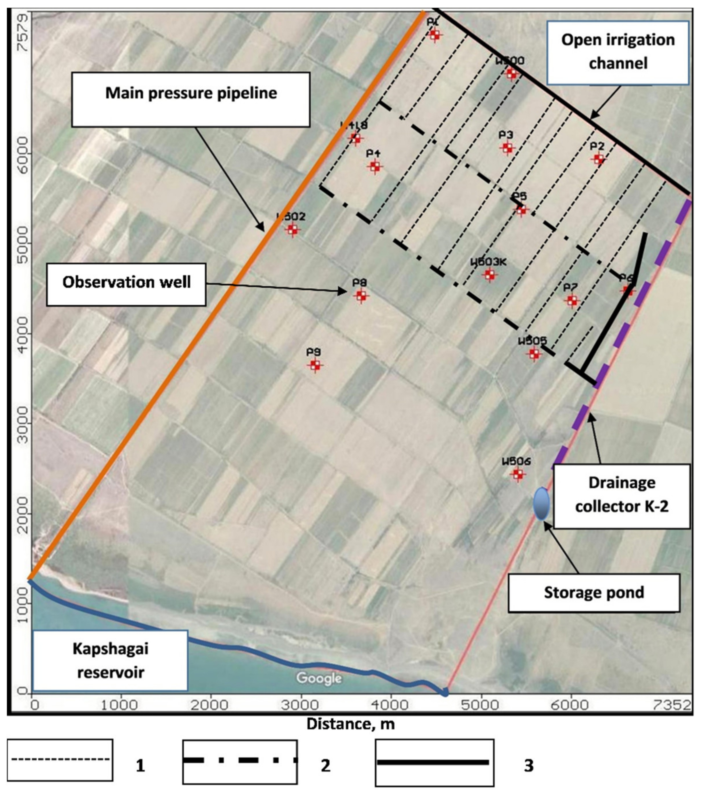
The collector-drainage system at the experimental site was installed on an area of 240 hectares in the northeastern part of the Shengeldy irrigation area. Horizontal subsurface drainage was made from polyethylene-perforated pipes with a diameter of 110–150 mm and installed at 2.3–2.8 m depth. The distances between drains are between 150–200 and 300–350 m, with a total horizontal subsurface drainage length of 10,895 m. Drainage water is collected in perforated asbestos-cement pipes (close collector) with diameters of 200–400 mm, installed at 2.5–3.2 m depth and with a total length of 3985 m. The drainage water from the close collector flows into the open collector K-2 and from there into a storage pond (Figure 2). Groundwater observation wells monitor the drainage flowing to the storage pond from late June to the end of the year. The total drainage water volume is from 700 to 1500 thousand m3, depending on the annual precipitation amount and the Kapshagai reservoir hydrological regime.
While the highest drainage water salinity reached 2.8 g/L, in the storage pond it was 1.1 g/L. The collector-drainage water chemical composition varies seasonally, with the highest salts concentration in the winter, with values 1.5–3.0 times higher than in the summer. The Kapshagai reservoir management determines the groundwater level fluctuation magnitude and the regional discharge during the crop irrigation period. Local actions such as deliberate or accidental drainage system outlet blocking gradually fill the drainage pipes and replenish the aquifer, raising the groundwater table and forming an additional irrigation volume either by pumping groundwater to the irrigation system or, once the groundwater level capillary fringe reaches the crop root zone, by moistening. This strategy is valid whenever the groundwater table is deeper than 1.5 m from the surface; otherwise, the crop root system might be harmed. Recharge reduction, for that matter, can act as active drainage and pumping for groundwater-piling reduction [21].
The Shengeldy irrigation area is 14,108 ha, although for crop production only 7710 ha or 54.6% of the total area is used. The sown area crops are mainly soybeans, onions, and cereal (Figure 3). Water from the Kapshagai reservoir flows by gravity through 1000 mm diameter pipes into four pumping station chambers, from where it is pumped into pressure pipelines. Water to the distribution network is supplied via pressure pipelines with diameters from 800 to 1200 mm, made of steel and asbestos cement, and then by a reinforced concrete channel network to the fields. The distribution network is built of LR-60 and LR-80 parabolic trays with a throughput of up to 0.45 m3/s. The trays are equipped with water outlets at 730–780 m intervals, from which water is supplied to the outlet furrows and further to irrigation furrows and strips.
Each year, 3100 to 3300 million m3 is taken for crop irrigation water and between 2600 and 2800 million m3 for household water supply. The annual irrigation system water loss is at least 500 million m3, which motivated the installation of water-saving irrigation technology [28]. The Israeli- and Chinese-made drip irrigation technologies and equipment that are used in 900 ha of onion and potato fields were found to intensify soil salinization [29].
2.2. Modeling Setup
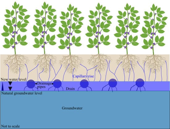
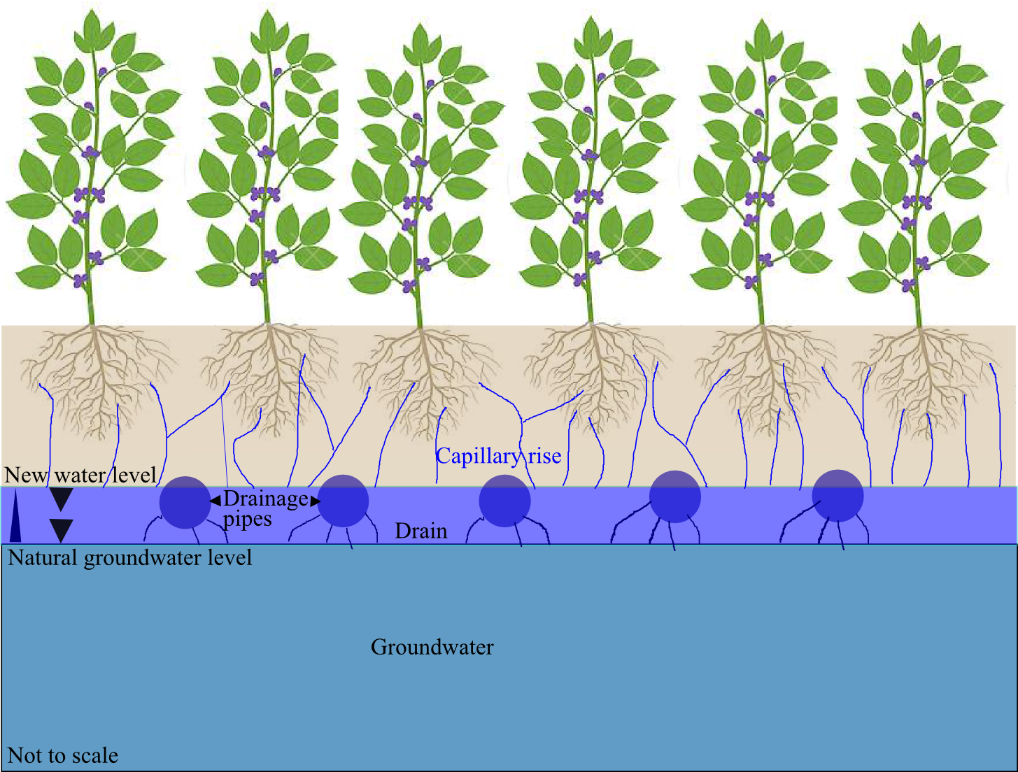
The concept of this study is that the drainage system hillock will raise the groundwater table during irrigation owing to drainage water filtration [30] to a level at which the capillary rise can supply moisture to the crop root system, which would thus make it possible to sustain water-demanding crop cultivation (such as soybeans, sugar beets, and forage crops, like alfalfa agriculture). This approach was tested by blocking the piped drainage to the open collector K-2 in the middle of the growing season, thereby creating a groundwater hillock underdrain. The drainage system potential for crop root system moistening was further evaluated by groundwater computer modeling method integration and field measurement.
2.2.1. Hydrogeological Survey
A hydrogeological conditions survey was conducted to evaluate the groundwater properties, dynamics, and parameters required to perform the geo-filtration modeling. The hydrogeological survey included:
- Drilling and installation of nine observation piezometers (indicated by the letter Pin Figure 2), each 7 m deep. All piezometers were equipped with a slit filter and gravel filling surrounding them at a depth interval of 3 to 5 m;
- To study the sediment cover and the unsaturated zone hydrophysical and mechano-physical properties, eight test sites consisting of shallow observation wells and equipped with nitrometers and moisture meters were prepared;
- Groundwater level and salinity monitoring in the six monitoring wells (indicated by the letter W in Figure 2) were performed monthly from January to April and from September to December. From May to August, every 10 days in the first and third quarters (April, May, and October), as well as four times a month from June to September; monitoring was done in observation piezometers,
- The groundwater hydro-chemical regime and irrigation effect were studied by water solution chemical analyses, including pH, Ca, Mg, Na + K, Cl, SO4, and HCO3 concentrations; total dissolved solids (TDS); and the sodium adsorption ratio (SAR). Water sampling was done in May, August, and October (i.e., in the beginning, closer to the end of the growing season, and during the opening of the damper on the K-2 collector);
- The field measurement database included rainfall and irrigation regimes, drainage water discharge, and evaporation potential. The database was compiled in 2016 and based on reported data of the Zonal Hydrogeological-Ameliorative Center of the Ministry of Agriculture, Republic of Kazakhstan, beginning from 2012 [5].
2.2.2. The Site Mathematical Computer Modeling Structure
The mathematical model represented the groundwater flow using a two-dimensional partial differential equation of groundwater flow through porous soil material in a one-layer geo-filtration system to an unconfined aquifer.
For the Quaternary aquifer, the flow equation [21] is as follows:
where Kx and Ky = the hydraulic conductivity along the x- and y-coordinate axes, respectively, which are the principal permeability directions; H = the potentiometric head; ηx and ηy = the elevation of the unconfined aquifer floor along the x- and y-coordinate axes; W = the fluxes representing recharge, evaporation, and drains; Sy = the specific yield of the porous material; and t = time. For steady-state conditions, the right side of Equation (1) equals zero (Sy(∂H/∂t = 0).
∂/∂x[Kx(Hx−ηx)(∂H/∂x)] + ∂/∂y[Ky(Hy−ηy)(∂H/∂y)] ± W = Sy(∂H/∂t)
Equation (1), with the boundary conditions below and an initial head condition specification, provided a mathematical model representation of the groundwater flow for the study area. The model boundary conditions were represented as head and flow, with their combination described in the following sections.
To represent the experimental site’s spatial variability, the area was overlaid with a grid, with each cell representing a point in the center of that cell. The grid was applied to the layer that characterizes the hydrodynamic and geological changes through the soil cross-section. The Shengeldy irrigation area experimental site groundwater model was constructed using Visual MODFLOW, which is an integrated computer program package for three-dimensional groundwater flow simulations based on physical laws of groundwater flow and mass transport in porous media. It is a widely used software package due to its easy access, relatively low cost, user-friendliness, and capability for transient/steady groundwater flow, simulating complex hydraulic conditions with various natural hydrological processes and/or artificial activities [8]. Visual MODFLOW can calculate flow fluxes across cell boundaries and predict groundwater head distribution in space and time. Hence, the Visual MODFLOW software package was selected in the present study. Groundwater head map contours and groundwater level depths from the soil surface were created using the MODFLOW software package’s instrumental identification and task-solving capabilities [32].
2.2.3. Model Illustration
Following the mathematical model’s approval, a computer model consisting of one horizontal layer was built for the Quaternary unconfined aquifer. The bottom boundary of the model was the roof of the Neogene Ily formation dense clays, adopted as an impermeable boundary. A computer model of the experimental site was created within the following boundaries (Figure 2). The model’s western boundary runs along the main pressure pipeline from the Kapshagai reservoir coast in the south to the open irrigation channel L9 in the north. The northern boundary of the experimental site model goes along L9 to the drainage collector K-2 in the east. The model’s eastern boundary extends from the north along with the drainage collector K-2, the storage pond, and further to the Kapshagai reservoir coast. The model’s southern boundary goes along the reservoir water line. Thus, the model considers the influence of the Kapshagai reservoir water level change on groundwater. The model region was divided into a rectangular grid with 65 × 68 computational cells. The grid steps along the axes were uneven and varied from 189 to 96 m along the x-axis and from 183 to 95 m along the y-axis. Thus, the maximal computing cell area was 3.5 ha, and the minimum was 0.9 ha. The minimal computational grid step was applied for the experimental site area itself, where detailed information was required, and the maximal grid step to the southern region of the model outside the experimental site. The origin of the model coordinates was in the lower-left corner of the rectangular region and corresponded to a point with the geographical coordinates 43.919734 N and 77.411448 Е. The actual geo-filtration area configuration was emphasized by defining inactive blocks outside its external borders.
The model boundary conditions were set as (Figure 4):
- The groundwater flow rate to the aquifer through the northern border, as recharge in the boundary blocks of the model;
- The existing subsurface drainage;
- Irrigation water infiltration during the irrigation period, as recharge in the corresponding blocks of the model;
- Evapotranspiration;
- The water level in the Kapshagai reservoir;
- Rain precipitation from April to November 2017.
The groundwater flow rate input to the model through the northern boundary was calculated according to hydrodynamic gradients, the flow cross-section, and the aquifer’s hydraulic conductivity. The total flow rate input to the model through the northern boundary was 208.6 thousand m3/year, which, once normalized to the total boundary blocks area, amounted to annual recharge of 772 mm, which was taken as constant during the model calculations. The initial distribution of the aquifer’s hydraulic conductivity values in the model was based on the field experimental pumping tests from observation wells. According to the pumping results, the hydraulic conductivity values varied from 1.12 m/day (well 505) up to 6.41 m/day (well 503 k). For the other wells, in most of the territory, the values of the hydraulic conductivity varied from 2.7 m/day up to 3.9 m/day. The subsurface drainage system was simulated by setting the boundary conditions of the third type (Figure 4) into the model as linear boundaries according to the drainage pipes’ locations, and it is presented as consecutive model blocks. To enable the use of linear boundaries, the initial and final depth values of each drain were set to calculate a linear-gradient intermediate depth along the borderline. The Drain Boundary Package supported Visual MODFLOW to simulate the balance between the drains and aquifer according to the difference between the aquifer dynamic head and the elevation of the drain [32]. The proportionality constant (drain conductance) value depends on the convergent flow pattern characteristics of the flow toward the drain and on the characteristics of the drain itself and its immediate environment [33].
The Drain Boundary Package assumes that the drains run partly full, so the water head within the drains is approximately equal to the median drain elevation. It was assumed that once the regional aquifer was depleted and its water table was below the drain’s elevation, no groundwater flow into the drain would occur and they would not affect the aquifer heads, as the entire region’s drainage percolates into it and the regional recharge to depletion ratio is much larger than that of each drain [33].
The groundwater spatial recharge from rainfall and irrigation percolation from the soil surface was entered as an input in the Visual MODFLOW Recharge Package [32]. This component was set in the model by zones according to the sown crop location. For assigning summer precipitation infiltration and recharge, 10% of the monthly measured values were taken as the initial data, based on the results of the field water-balance experiments in the Shengeldy site [24]. The additional groundwater recharge by irrigation water infiltration was considered as 20% from the irrigation rate at the area under crops sown during the irrigation period (as the initial value). The total groundwater recharge value was subsequently adjusted at the calibration and model validation stages.
To simulate the groundwater table contribution to capillary rise, evaporation, and evapotranspiration, the Visual MODFLOW Evaporation Package was used [32]. The capillary fringe boundary condition assumes a linear relationship between evapotranspiration potential and the groundwater level. Groundwater withdrawal was calculated for each time step for the specific groundwater level depth. The evapotranspiration maximal value was calculated for water level at the surface, as the surface water evaporation value. With the groundwater level decreasing, the evapotranspiration flux also decreased linearly up to a depth until it was null [30]. The initial input values were based on local meteorological evaporation data and applied uniformly over the model area with a critical depth of 1.5 m. The evaporation values were set according to the 2017 monthly average from April to November, which varied from 138 mm/year for November to 1836 mm/year in August [5].
To assess the hydraulic connection between the Kapshagai reservoir water level and groundwater, the southern model boundary was simulated as a boundary condition of the first type (Figure 4) with a pressure head that matched the monthly average water level in the reservoir. The storage pond was also set as a boundary condition of the first type with a constant pressure head consistent with the pond’s annual average water level. The time step of the model was set in days from the beginning of the model’s calculation (start time—0 days), which was set to 25 April 2017—the beginning of the growing season and the beginning of the observations. Intermediate time steps were set automatically by the program, depending on the boundary condition change time and observation periods (stress periods).
To characterize the experimental site’s hydrodynamic groundwater flow grid, groundwater head contour maps were combined with the flow paths. Maps were built for three characteristic stages in 2017: 25 April, the beginning of the growing season; 15 July, the middle of the growing season; and 5 October, the end of the growing season and the end of irrigation.
2.2.4. Model Calibration and Validation
During the calibration, the model was adjusted until it closely simulated the measured historical performance of the modeled system. The model parameters for layer hydraulic conductivity values, aquifer storage coefficients, recharge, and drain conductance were adjusted and the water balance was evaluated. Steady-state modeling was used for consideration of boundary conditions and model parameters, as well as to simulate the general groundwater flow. During steady-state modeling, only natural boundary conditions (groundwater flow in the aquifer, averaged year precipitation, and hydraulic connection between the Kapshagai reservoir water level and groundwater) were calculated. There were no significant trends in groundwater heads and water levels in the Kapshagai reservoir. The groundwater head in April 2017 was used to assign the initial head for the steady-state modeling.
For the no-steady-state (time-varying) phases, the model was run from 15 April 2017 to 15 November 2017, during which the actual system behavior was observed. The model was run with time steps automatically chosen by the Visual MODFLOW program over the period that covered the full hydrological cycle, including rainfall, irrigation, and any other typical changes in the groundwater regime. Wherever simulated water level and pressure behavior did not match the observed behavior, careful adjustments were progressively made to the model’s hydraulic conductivity and recharge value layers assigned to characterize the relevant cells. Model calibration was continued until an acceptably close match between simulated and observed behaviors was achieved. Considering that the observed groundwater head elevation spatial difference was 45 m and annual groundwater head fluctuations were on average 4.0 m, the model’s calibration of acceptable accuracy in terms of water levels was defined as ±0.5 m and in terms of groundwater budget components, it was defined as ±5%. For model validation, the coincidence of the water balance elements and geo-filtration parameters obtained from the data of field measurements and calculated for the model was also considered.
2.2.5. Model Predictions
The calibrated model was applied to simulate and predict a scenario in which surplus irrigation would be collected by the drainage system as additional groundwater recharge. In cases of drainage system output blockage, water would gradually fill the drainage pipe volume and, when filled, percolate back to the aquifer. Since this idea is controversial, it was decided to assess it by modeling such a scenario. The initial data for the prediction model were the balance calculation results performed on the calibrated and validated model. Balance zones were selected along the lower part of the K-2 drainage collector and the southern (the lowest downstream) main subsurface drain, where the groundwater level was being lowered more than the subsurface drainage depth. Based on the selected zone balance calculations, drainage areas were determined and model cell boundary conditions were regarded as “outflow”. The flow rate in these cells was determined, as well as the time of its arrival. Based on this flow rate and cell area, an additional recharge in mm/year was calculated and added to the corresponding recharge zones that were determined at the model’s identification stage.
3. Results
3.1. Model Calibration
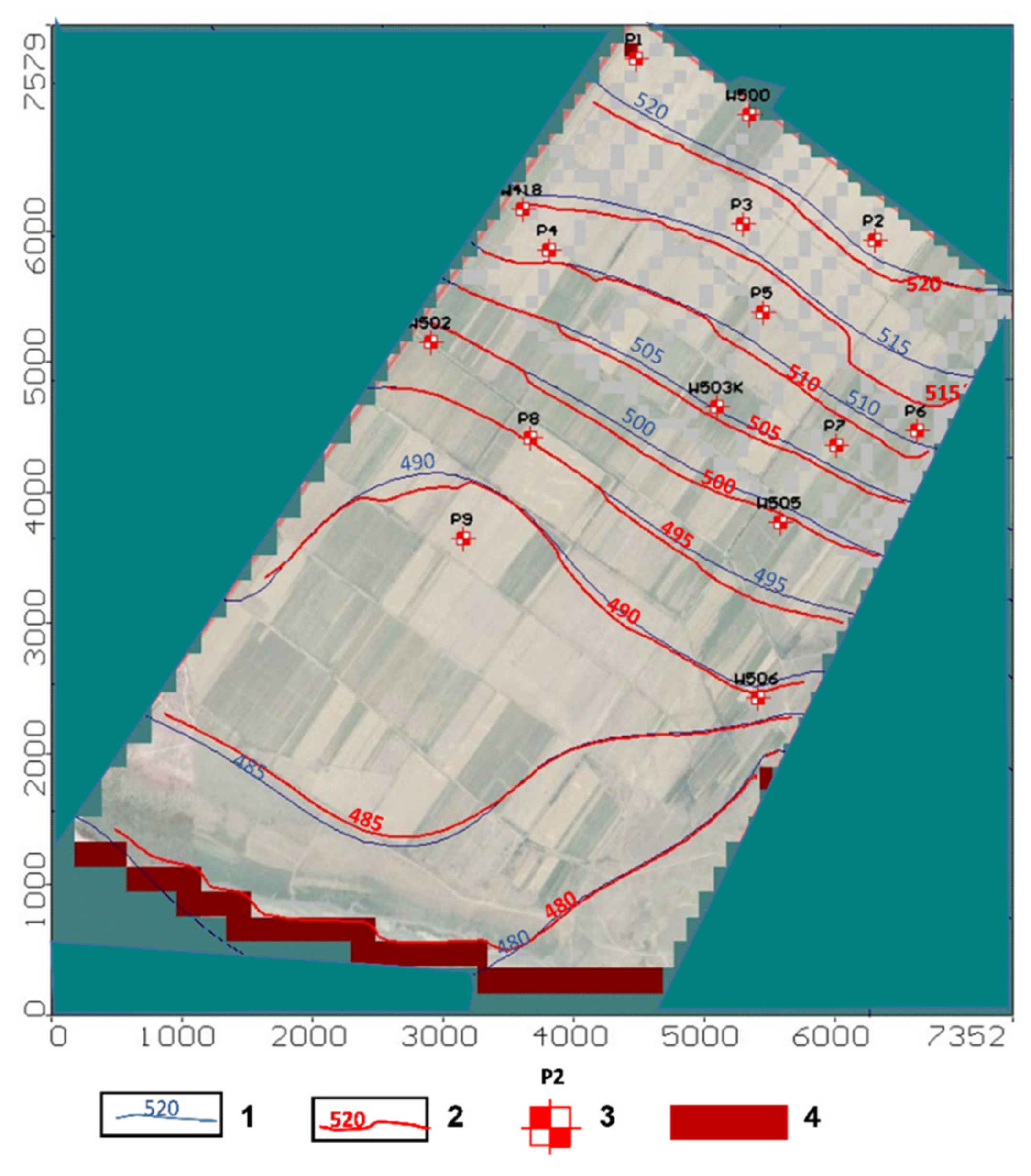
The results of the analyses of the model sensitivity towards parameter changes indicated that the model could recognize changes in specific storage (initial values ±15%) and in the layers’ hydraulic conductivity (initial values ±50%). The model was more sensitive to recharge. Comparison of the initial groundwater head, measured in the observation wells on 25 April 2017, and the model-calculated ones showed a good agreement (less than ±0.5 m) between the observed water levels in observation well 4 and the Kapshagai reservoir and the results modeled with the steady-state simulation (Figure 5). The calibrated hydraulic conductivity of the aquifer was found to range from 1.7 to 5.7 m/day. In most of the territory, the values of the calibrated hydraulic conductivity were 3.1 m/day, which was in good agreement with the values obtained from the field studies and experimental pumping from wells (Section 2.2.3).
The recharge in the aquifer was calibrated as 109 mm or 24.9% of the annual rainfall in 2016 (437 mm). In the next step of the model calibration, transient flow (no-steady-state) was simulated. At this stage of model calibration, attention was mainly paid to determining the areal recharge and discharge of groundwater due to the infiltration of irrigation water and precipitation.
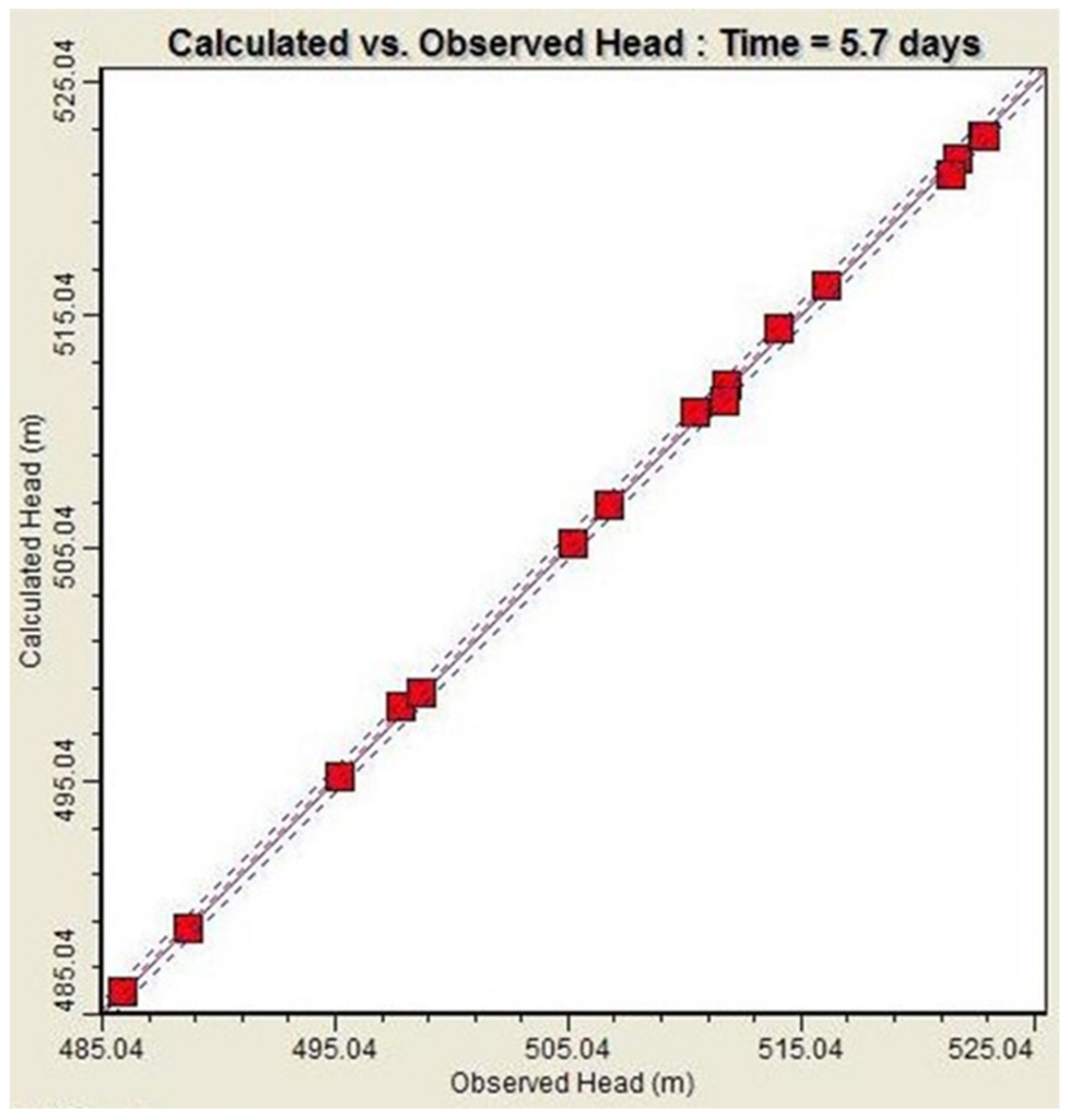
The residual mean was 0.083 m, the absolute residual mean was 0.21 m, the estimated standard error was 0.06 m, and the root means squared (RMS) was 0.255 m. In addition, the correlation coefficient between the measured and model groundwater levels was 1.0 (Figure 6). Comparison of the measured groundwater level fluctuations and the model-calculated ones showed a good agreement (less than ±0.5 m) between the observed and modeled results for observation piezometers (Figure 7) as well as for the continuous monitoring wells (Figure 8).
The total water volume supplied through the irrigation systems in the 2017 growing season was 16.03 million m3. The groundwater model calculated recharge was 9.11 million m3, which, when considering that the total groundwater input through the outer border was 2.9 million m3, the precipitation infiltration was 2.52 million m3 and the total irrigation water loss was 3.69 million m3, amounted to 40.5% of the irrigation water supply.
3.2. Model Validation
The initial drain conductance values were calculated from the measured drainage flow rate values and the difference between the aquifer water head and the drain elevation, and they were found to be 1.5–2.5 m2/day. The general direction of the groundwater flow coincides with the relief slope in a south-south-west direction toward the Kapshagai reservoir. Although, the hydraulic gradient was the same at the beginning of the growing season, near the Kapshagai reservoir coast it gradually decreased so that drainage did not occur, as the K-2 drainage collector drained the groundwater flow to the reservoir. Before the intensive irrigation of the growing season, the experimental site’s groundwater depth varied from 4 to 6 m and even up to 8 m near the eastern border of the site. A higher groundwater level (2.5–1.5 m) was found in the southwestern region and at 2.5–3 km north from the Kapshagai reservoir coast, around a storage pond located in a lowered relief area. The groundwater hydraulic gradient became more uniform once irrigation started (Figure 9).
The water-saving and groundwater salinity balance datasets were obtained from groundwater level and soil salinity field observations [5]. In the middle of the growing season (15 July 2017), the irrigation infiltration losses began overlapping with the overall groundwater flow. The drain effect began to appear in the drainage system’s upper part, as indicated by a flow path direction change in the map (Figure 9). The groundwater level depth decreased significantly in the middle of the growing season to 3–5 m from the soil surface (Figure 10). The groundwater level rise was uneven owing to different crop irrigation intensities. The maximal groundwater level increase was observed in sugar beet and onion fields, where the groundwater level rose to a depth of 2.5—3.5 m from the soil surface.
In the pre-growing season, groundwater storage recharge depletion did not exceed the flow rate of 16 thousand m3/day, and in the first half of the growing season, it even decreased to 9.5 thousand m3/day (Table 1). However, in the second half of the growing season, it increased to 113 thousand m3/day and then decreased again to 76 thousand m3/day at the beginning of winter. Simultaneously, at the first half of the growing season, groundwater recharge sharply increased due to irrigation from 58.1 thousand m3/day to 117 thousand m3/day by the middle of the growing season, while toward the end of the growing season, it decreased and did not exceed 9.6 thousand m3/day. In the first half of the growing season, there was a significant increase in the groundwater operational storage replenishment from 56.9 thousand m3/day to 116 thousand m3/day, and then a sharp decrease to 6.6 thousand m3/day up to the end of the growing season.
In contrast, the surface discharge flow rate reached its maximal value in the growing season’s second half, with a value of 108 thousand m3/day. The recharge loss to evapotranspiration from the groundwater table was at its maximum in the hottest period of the year and ranged from 12 thousand m3/day to 9.1 thousand m3/day, while in November it decreased to 0.7 thousand m3/day. The groundwater flow to the Kapshagai reservoir was small and did not exceed 2 thousand m3/day. Considering that in the first half of the growing season the groundwater level was lower than the drainage depth, the maximal drainage outflow value was 1.6 thousand m3/day at the end of the growing season. As a result, the model accurately simulated the measured historical characteristics of the simulated system. The values of hydraulic conductivity, specific storage, recharge, drainage conductivity and water balance in the model agreed with the values obtained as a result of field experiments within the specified modeling accuracy.
3.3. Model Prediction
To evaluate identification prediction, detailed groundwater depth maps were created for the beginning, middle, and end of the growing season, as well as for the winter. Through comparison of the maps, it was found that additional recharge of groundwater from the drains gradually formed local groundwater-level rising zones along the drain. While drainage infiltration in the middle of the growing season was hardly noticeable, by the end of the growing season minor sites with groundwater depths of 1 to 2–2.5 m from the soil surface appeared (Figure 11) and, up to the beginning of the winter period, although irrigation stopped, drainage infiltration to the aquifer continued. As a result, a bigger area with a groundwater depth smaller than 1 m from the soil surface had formed.
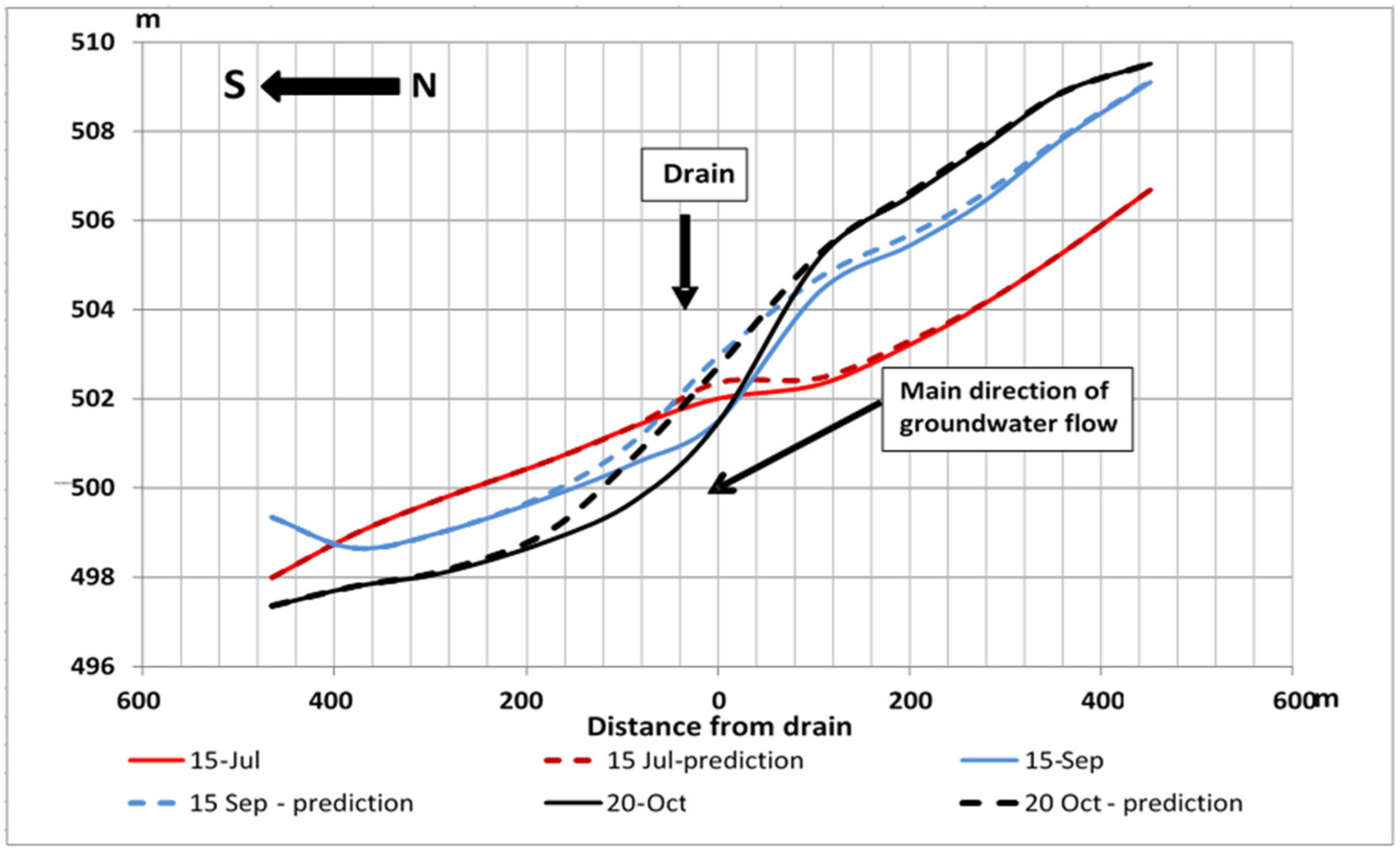
The groundwater level in the cross-section task results fluctuates over time compared to the additional groundwater recharge setting in the middle of the zone (Figure 12). In the middle of the growing season, the groundwater level additional elevation was directly above the drain and did not exceed 0.4 m, with an influence zone of approximately 100–120 m upstream and 80–90 m downstream. By the end of the growing season, the additional groundwater level rise was already 1.5 m, and this influence zone expanded to 300–350 m upstream and up to 200–250 m downstream.
3.4. Assessment of Additional Drainage Water Irrigation Source for Crop Root Zone Moisturizing
The capillary rise value varied from 0.6 m for crushed stone-gravel deposits with sandy loam aggregate to 2.5 m for light loams including finely crushed stone, averaging 1.5 m [24]. The soybean and sugar beetroot system penetration depth in the irrigated lands reached 2 m [34]. In a soybean field, the irrigation savings per hectare compared to previous years amounted to approximately 22%, with a planned soybean irrigation norm of 10,526 m3/ha compared to the actual use of 8246 m3/ha. As only one field was allocated for soybean, the savings amounted to 72,960 m3/ha, which could sustain approximately 10 additional hectares.
The vertical infiltration and capillary rise of weakly mineralized groundwater enriched the soybean root zone with minerals and other useful ingredients, which leads to in 2017 to a yield increase of 1.45 tons per hectare or 37% compared with the traditional irrigation regime in 2015 and 36% compared to 2016. In a sugar beet field, irrigation per hectare saved was approximately 18%, with a planned irrigation norm of 7456 m3/ha and anactual use of 6134 m3/ha. As only one sugar beet field was allocated, the savings amounted to 47,592 m3/ha, which could sustain about an additional 6.5 hectares. The sugar beetroot system artificial nourishment contributed to a yield increase of 31.5 tons per hectare or 12% compared with the traditional irrigation regime in 2015 and to 14% compared to 2016.
4. Discussion
The Shengeldy area irrigation from the Kapshagai reservoir relies on the Ily River water flow, which is completely dependent on neighboring China. However, the consistent increase in water withdrawal also causes water quality deterioration [35]. In addition, surface water over-development for arable land and other utilities in Kazakhstan depletes local water resources and restricts cross-border water resources to neighboring countries downstream of the Ily River [28]. The other urgent problems of water and soil pollution [36] and salinization are consequences of a regional desertification trend [29]. Such global climate change-related negative feedback trends are common to many regions undergoing aridification processes [37].
Since May 2014, the Ily River flow rate decreased from 291 m3/s to 90 m3/s and the water level in the Kapshagai reservoir decreased from 477 m to a critical level of 475 m, with an annual recharge volume of 13.3 cubic kilometers. In 2005, for comparison, the Ily River average flow rate was 585 m3/s, and the Kapshagai reservoir water level was 477 m, with a recharge volume of 16.3 cubic kilometers. In such a scenario, improving water resource management is essential and the work presented here supplies a potential methodology for water resource management optimization.
Our model calibration results represented the ratio between model-calculated and measured averaged groundwater levels and the observed and modeled recharge values that in all cases had a reasonable fit to the groundwater head contours. This indicates that the geo-filtration hydrogeological model and ameliorative conditions of the Shengeldy irrigation area experimental site met the specified requirements for model solution accuracy and reliability (Figure 5 and Figure 6). The model’s balance calculations indicated that the installed drainage system has low efficiency, considering the (deep) existing groundwater level (Figure 11), suggesting that outflow from the subsurface drainage system should also be ensured after irrigation ends. The additional groundwater recharge influence owing to drainage return to the aquifer was local due to the significant groundwater hydrodynamic gradient.
The asymmetry in the groundwater level between the two sides of the drain is caused by the supporting effect of additional recharge from the main groundwater flow. A groundwater flow balance comparison showed that due to the drainage water return, the total groundwater recharge in the experimental site at the end of the growing season increased by 146 thousand m3. Storage reserve replenishment increased by 40.6 thousand m3 and evapotranspiration by 4.5 thousand m3. The field study results for the Shengeldy irrigation area experimental site showed good groundwater recharge potential for the existing subsurface drainage as an additional irrigation source. In contrast to the common notion that capillary rise evapotranspiration is negligible [30], it was found that the capillary rim rising to the lower root-zone boundary was significant, thereby moisturizing crops during the growing season (Figure 1) and also contributing to evapotranspiration [17].
5. Conclusions
Owing to the Ily River flow rate reduction and high evaporation rates from the reservoirs (Wu et al., 2019), groundwater levels in the southern Shengeldy irrigation area fell below the drainage pipes and part of the drainage flow began to percolate into the underlying sediments. Under the current scenario, in the event of drainage system output blockage, the drainage pipes will gradually fill and replenish the aquifer, thereby forming an additional source of groundwater recharge that can be used as an effective alternative source for moisturizing and feeding the crop root zone.
Under such conditions, a proper irrigation scheme that sustains crop growth and flushes excessive salts is crucial, with a shift from traditional to drip irrigation systems [29]. Utilization of existing drainage systems for agricultural hydrologic balancing was tested in the Shengeldy irrigation area by partially blocking the K-2 collector drainage in the middle of the growing season, thereby creating additional local increase in the groundwater level. This field experiment was also used for training, testing, and validating a MODFLOW model built for predicting the method’s application in various locations and scenarios. The modeling results imply that:
- The MODFLOW spatial distribution groundwater flow model provided reliable information about artificial groundwater recharge from existing drainage in complex hydrogeological and intensive farming conditions. The hydrogeological and ameliorative conditions of the geo-filtration model for the experimental site of Kazakhstan’s Shengeldy agricultural area were based on and validated by field study results and met the specified model solution accuracy and reliability requirements;
- The model’s additional groundwater recharge prediction due to existing drainage infiltration under the current irrigation conditions was validated against experimental data obtained at the site in 2017. It was found that at the end of the growing season, the groundwater table’s additional elevation from drainage infiltration would be about 1.5 m below the drains, and the additional groundwater recharge influence zone would spread to up to 350 m from the drains.
- Based on the simulation results, detailed groundwater head contour maps and flow paths, as well as groundwater table depths from the soil surface, were made for typical periods of irrigation. The groundwater flow balances that were calculated in the model for the same periods made it possible to quantify and characterize the temporal change in the groundwater flow balance. The calculated irrigation water infiltration loss reached 40.5% of the irrigation water supply.
- The experimental study and field monitoring results confirmed the MODFLOW simulation, showing that under certain conditions drainage can be an additional source of irrigation. Furthermore, through the artificial use of groundwater capillary rise to the lower root system boundary, crop nourishing and moisturizing can be obtained during the growing season.
- Agriculture is an important sector in the economy of Central Asia that is restricted by water scarcity [17]. The new capillary fringe irrigation approach presented in this paper can more than double the arable land in Kazakhstan and neighboring countries. Seasonal undulation in the groundwater level is necessary to prevent accumulation of salts in the soil section [37].
Author Contributions
V.M.: methodology, modeling, writing—original draft preparation, V.K.: methodology, preparing data for modeling, writing, field investigation; A.M.: writing, modeling, field investigation; E.K.: writing, investigation; Y.A.: writing—reviewing and editing, conceptualization. All authors have read and agreed to the published version of the manuscript.
Funding
This research received no external funding.
Institutional Review Board Statement
Not applicable.
Informed Consent Statement
Not applicable.
Data Availability Statement
Data supporting the reported results can be found in the Hydroshare repository: https://www.hydroshare.org/resource/4ed6ba940caf42a7bc4ba8ce9dfade8a/ (accessed on 15 August 2021.)
Acknowledgments
The authors want to thank Ilan Shakibaev, the Head of the Zonal Hydrogeological-Ameliorative Center of the Ministry of Agriculture, Republic of Kazakhstan, for providing reporting materials concerning monitoring observations of the groundwater regime, soil-water laboratory tests for creating hydrogeological maps, as well as the results of irrigation and drainage surveys performed on the Shengeldy irrigation area. Thanks also go to Gulsara Kerimbaeva, the Head of the Shengeldy Department for Monitoring Irrigated Lands of the Zonal Hydrogeological-Ameliorative Center, for providing practical assistance in organizing and conducting field investigations on the experimental site of the Shengeldy Irrigation Area. Furthermore, we thank Michael Maoz from Ariel University for his help with language editing.
Conflicts of Interest
The authors declare no conflict of interest.
References
- Rhoades, J.D.; Bingham, F.; Letey, J.; Hoffman, G.; Dedrick, A.; Pinter, P.; Replogle, J. Use of saline drainage water for irrigation: Imperial Valley study. Agric. Water Manag. 1989, 16, 25–36. [Google Scholar] [CrossRef]
- Aljenaby, A.Z.A.; Aljenaby, Z.A.Z. Usage of drainage water in irrigation: Applications on the eastern euphrates in Babylon province. Int. J. Agric. Stat. Sci. 2018, 14, 331–338. [Google Scholar]
- Nindwani, B.A.; Lashari, B.K.; Memon, A.A.; Laghari, K.Q.; Hammad, H.M.; Farhad, W. Impact of drainage water use for crop irrigation. Sci. Int. 2014, 26, 273–278. [Google Scholar]
- Valipour, M. Effect of Drainage Parameters Change on Amount of Drain Discharge in Subsurface Drainage Systems. IOSR J. Agric. Vet. Sci. 2012, 1, 10–18. [Google Scholar] [CrossRef]
- Kulagin, V.; Umbetaliev, D.; Auelkhan, Y.; Makyzhanova, A.; Karataev, D. Groundwater water-salt balance of shengeldy irrigated lands using water-saving technologies. News Natl. Acad. Sci. Repub. Kazakhstan, Ser. Geol. Tech. Sci. 2017, 3, 161–174. [Google Scholar]
- Sanford, W. Recharge and groundwater models: An overview. Hydrogeol. J. 2002, 10, 110–120. [Google Scholar] [CrossRef]
- Hashemi, H.; Berndtsson, R.; Persson, M. Artificial recharge by floodwater spreading estimated by water balances and groundwater modeling. Hydrol. Sci. J. 2015, 60, 336–350. [Google Scholar] [CrossRef]
- Rejani, R.; Jha, M.K.; Panda, S.N.; Mull, R. Simulation modeling for efficient groundwater management in balasore coastal basin, India. Water Resour. Manag. 2008, 22, 23–50. [Google Scholar] [CrossRef]
- Mirlas, V.; Antonenko, V.; Kulagin, V.; Kuldeeva, E. Assessing artificial groundwater recharge on irrigated land using the MODFLOW model. Earth Sci. Res. 2015, 4, 16. [Google Scholar] [CrossRef]
- Mirlas, V. MODFLOW Modeling to Solve Drainage Problems in the Argaman Date Palm Orchard, Jordan Valley, Israel. J. Irrig. Drain. Eng. 2013, 139, 612–624. [Google Scholar] [CrossRef]
- Sarwar, F.; Feddes, R.A. Evaluating drainage design parameters for the fourth drainage project, Pakistan by using SWAP model: Part II- Modeling results. Irrig. Drain. Syst. 2000, 14, 281–299. [Google Scholar] [CrossRef]
- Gates, T.K.; Burkhalter, J.P.; Labadie, J.W.; Valliant, J.C.; Broner, I. Monitoring and modeling flow and salt transport in salinity-threatened irrigated valley. J. Irrig. Drain. Eng. 2002, 128, 87–99. [Google Scholar] [CrossRef]
- Kurien, V.M.; Cooke, R.A.; Hirshi, M.C.; Mitchell, J.K. Estimating drain spacing of incomplete drainage system. Trans. ASAE 1997, 40, 377–382. [Google Scholar] [CrossRef]
- Singh, R.; Helmers, M.J.; Zhiming, Q. Calibration and validation of DRAINMOD to design subsurface drainage system for Iowa’s tile landscapes. Agric. Water Manag. 2006, 65, 221–232. [Google Scholar] [CrossRef]
- Bradford, R.B.; Acreman, M.C. Applying MODFLOW to wet grassland in-field habitats: A case study from the Pevensey Levels, UK. Hydrol. Earth Syst. Sci. 2003, 7, 43–55. [Google Scholar] [CrossRef] [Green Version]
- Sagin, J.; Adenova, D.; Tolepbayeva, A.; Poryadin, V. Underground water resources in Kazakhstan. Int. J. Environ. Stud. 2017, 74, 386–398. [Google Scholar] [CrossRef]
- Ostrovsky, V.N. Comparative analysis of groundwater formation in arid and super-arid deserts (with examples from central Asia and northeastern Arabian Peninsula). Hydrogeol. J. 2007, 15, 759–771. [Google Scholar] [CrossRef]
- Zhupankhan, A.; Tussupova, K.; Berndtsson, R. Water in Kazakhstan, a key in Central Asian water management. Hydrol. Sci. J. 2018, 63, 752–762. [Google Scholar] [CrossRef] [Green Version]
- Mukhamedzhanov, M.; Makyzhanova, A.; Kulagin, V. The rationale and definition of prospects by the use of groundwater for irrigation, forage production and pastures irrigation of Kazakhstan. News Nat. Acad. Sci. Rep. 2017, 3, 72–83. [Google Scholar]
- Ring, I.; Sandström, C. Chapter 6: Options for governance and decision-making across scales and sectors. Regional and Subregional Assessments of Biodiversity and Ecosystem Services: Regional and Subregional Assessment for Europe and Central Asia; Bonn, Germany, 2018; Volume 9, pp. 1–587. Available online: https://jyx.jyu.fi/handle/123456789/62146 (accessed on 10 August 2021).
- Belitz, K.; Phillips, S.P. Alternative to Agricultural Drains in California’s San Joaquin Valley: Results of a Regional-Scale Hydrogeologic Approach. Water Resour. Res. 1995, 31, 1845–1862. [Google Scholar] [CrossRef]
- Pueppke, S.G.; Nurtazin, S.T.; Graham, N.A.; Qi, J. Central Asia’s Ili River ecosystem as a wicked problem: Unraveling complex interrelationships at the interface of water, energy, and food. Water 2018, 10, 541. [Google Scholar] [CrossRef] [Green Version]
- Wu, H.; Wu, J.; Song, F.; Abuduwaili, J.; Saparov, A.S.; Chen, X.; Shen, B. Spatial distribution and controlling factors of surface water stable isotope values (δ 18 O and δ 2 H) across Kazakhstan, Central Asia. Sci. Total Environ. 2019, 678, 53–61. [Google Scholar] [CrossRef]
- Makyzhanova, A. Groundwater Resources of Kazakhstan and Water Supply Tasks for Agrarian Sector of the Economy (State, Prospects); Kazakh National Research Technical University: Almaty, Kazahstan, 2018. [Google Scholar]
- Thevs, N.; Nurtazin, S.; Beckmann, V.; Salmyrzauli, R.; Khalil, A. Water consumption of agriculture and natural ecosystems along the Ili river in china and kazakhstan. Water 2017, 9, 15. [Google Scholar] [CrossRef] [Green Version]
- Dzhetimov, M.; Andasbayev, E.; Esengabylov, I.; Koyanbekova, S.; Tokpanov, E. Physical and Chemical Research of Processes of Salt Formation in the Water of Balkhash Lake. In Proceedings of the CBU International Conference Proceedings, Prague, Czech Republic, 30 June 2013; Volume 1, pp. 400–411. [Google Scholar]
- Gulnura, I.; Abuduwaili, J.; Oleg, S. Deflation processes and their role in desertification of the southern Pre-Balkhash deserts. Arab. J. Geosci. 2014, 7, 4513–4521. [Google Scholar] [CrossRef]
- Ding, Y.K.; Li, Y.P.; Liu, Y.R. Spatial-temporal assessment of agricultural virtual water and uncertainty analysis: The case of Kazakhstan (2000–2016). Sci. Total Environ. 2020, 724, 138155. [Google Scholar] [CrossRef] [PubMed]
- Wang, Z.; Fan, B.; Guo, L. Soil salinization after long-term mulched drip irrigation poses a potential risk to agricultural sustainability. Eur. J. Soil Sci. 2019, 70, 20–24. [Google Scholar] [CrossRef] [Green Version]
- Alemie, T.C.; Tilahun, S.A.; Ochoa-Tocachi, B.F.; Schmitter, P.; Buytaert, W.; Parlange, J.; Steenhuis, T.S. Predicting Shallow Groundwater Tables for Sloping Highland Aquifers. Water Resour. Res. 2019, 55, 11088–11100. [Google Scholar] [CrossRef]
- Kruseman, G.P.; de Ridder, N. Analysis and Evalution of Pumping Test Data; International Institute for Land Reclamation and Improvement: Wageningen, The Netherlands, 1994. [Google Scholar]
- Schlumberger Water Services. Visual MODFLOW 2011.1 User’s Manual; Schlumberger Water Services: Kitchener, ON, Canada, 2011. [Google Scholar]
- Zipper, S.C.; Dallemagne, T.; Gleeson, T.; Boerman, T.C.; Hartmann, A. Groundwater Pumping Impacts on Real Stream Networks: Testing the Performance of Simple Management Tools. Water Resour. Res. 2018, 54, 5471–5486. [Google Scholar] [CrossRef] [Green Version]
- Kaspar, T.C.; Stanley, C.D.; Taylor, H.M. Soybean Root Growth during the Reproductive Stages of Development 1. Agron. J. 1978, 70, 1105–1107. [Google Scholar] [CrossRef]
- Stone, R. For China and Kazakhstan, no meeting of the minds on water. Science 2012, 337, 405–407. [Google Scholar] [CrossRef]
- Ramazanova, E.; Lee, S.H.; Lee, W. Stochastic risk assessment of urban soils contaminated by heavy metals in Kazakhstan. Sci. Total Environ. 2021, 750, 141535. [Google Scholar] [CrossRef] [PubMed]
- Pandit, R.; Parrota, J.; Anker, Y.; Coudel, E.; Diaz Morejón, C.F.; Harris, J.; Karlen, D.L.; Kertész, Á.; Mariño De Posada, J.L.; Ntshotsho Simelane, P.; et al. Chapter 6: Responses to Halt Land. In IPBES. The IPBES Assessment Report on Land Degradation and Restoration; Montanarella, L., Scholes, R., Brainich, A., Eds.; Secretariat of the Intergovernmental Science-Policy Platform on Biodiversity and Ecosystem Services: Bonn, Germany, 2018; pp. 435–528. [Google Scholar]
Figure 1.
Shengeldy irrigation area location.
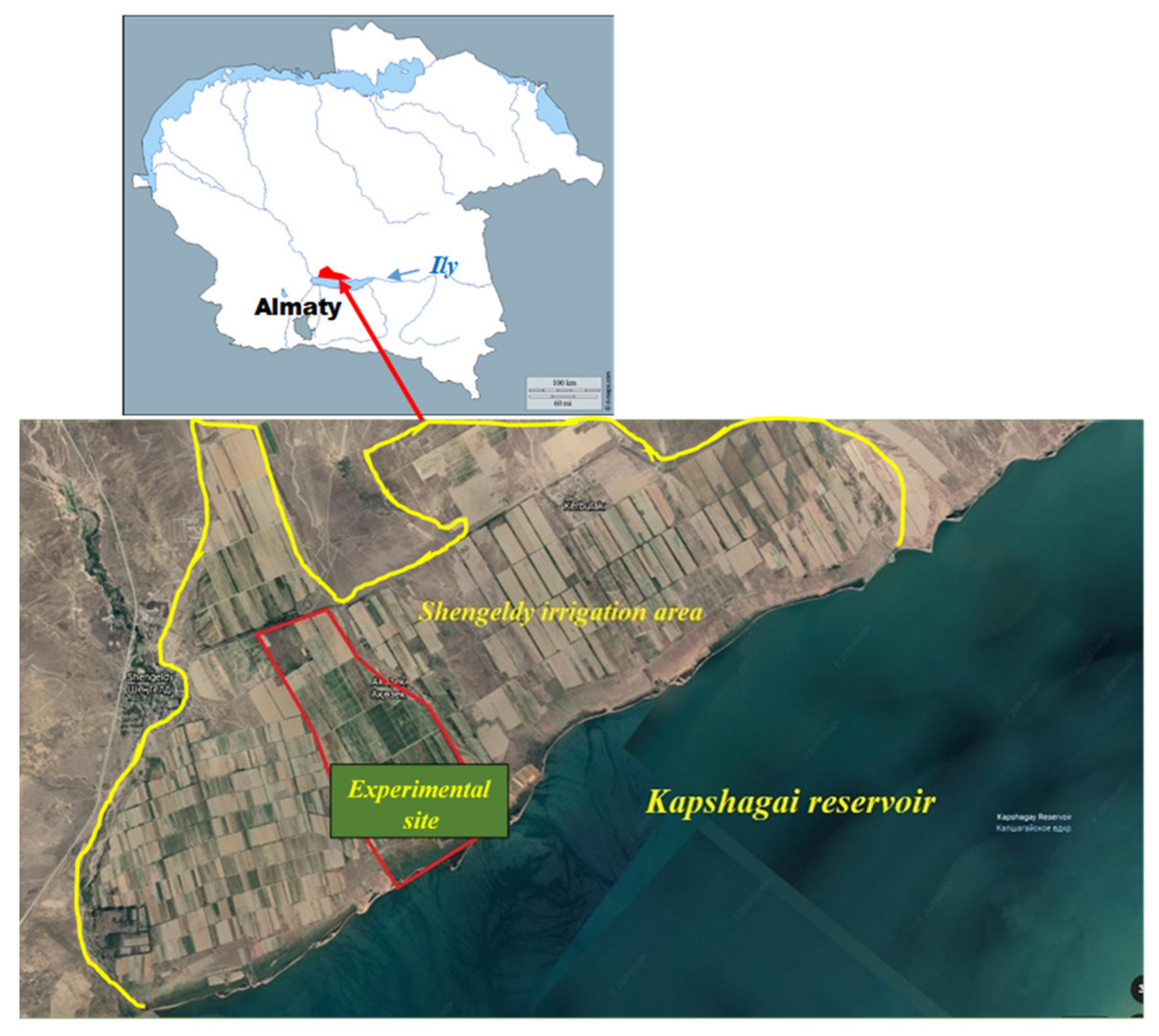
Figure 2.
The experimental site collector-drainage system: (1) horizontal subsurface drainage; (2) main subsurface drainage; (3) close collector.
Figure 2.
The experimental site collector-drainage system: (1) horizontal subsurface drainage; (2) main subsurface drainage; (3) close collector.

Figure 3.
The structure of crop distribution in the Shengeldy irrigation area in 2016.
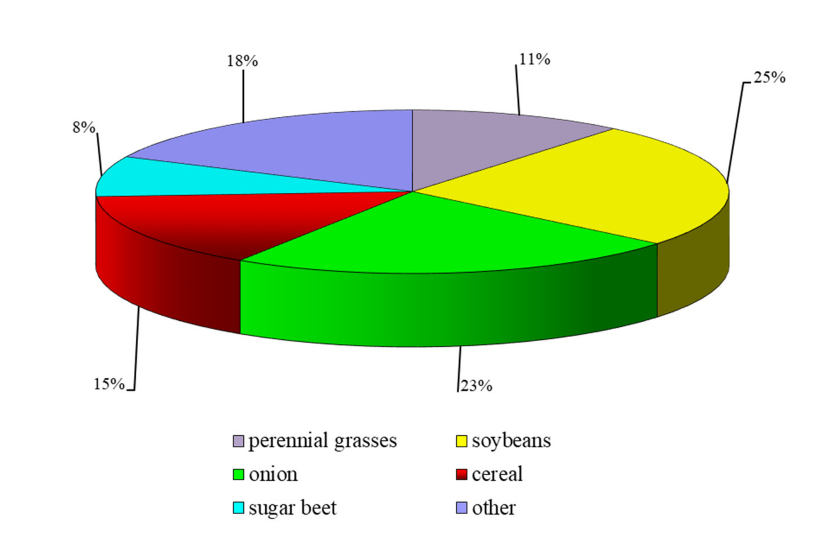
Figure 4.
The Shengeldy irrigation area experimental site: model grid and boundary conditions. The legend numbers indicate the following locations on the map: 1 = observation well; 2 = boundary condition, first type; 3 = existing drains; 4 = active cells; 5 = inactive cells (no flow within the model domain).
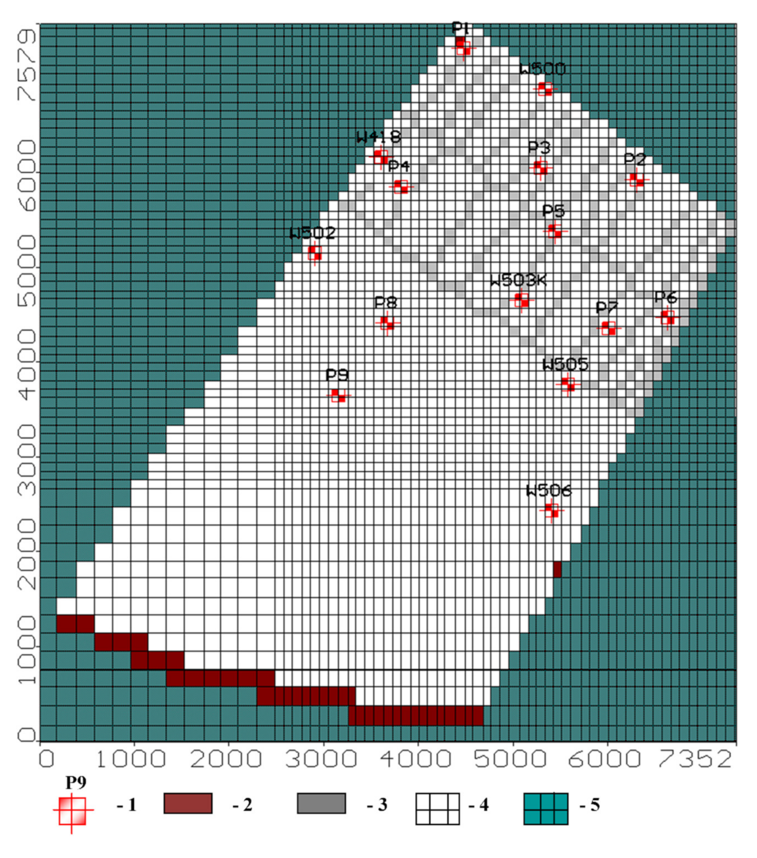
Figure 5.
Comparison of the initial groundwater head and the model-calculated ones. Results of the steady-state simulation: 1—initial groundwater head; 2—model-calculated groundwater head; 3—observation well; 4—Kapshagai reservoir (first-type boundary condition).
Figure 5.
Comparison of the initial groundwater head and the model-calculated ones. Results of the steady-state simulation: 1—initial groundwater head; 2—model-calculated groundwater head; 3—observation well; 4—Kapshagai reservoir (first-type boundary condition).

Figure 6.
Comparison between model-calculated and measured averaged groundwater levels in the observation wells.
Figure 6.
Comparison between model-calculated and measured averaged groundwater levels in the observation wells.

Figure 7.
Model calibration vs. observed groundwater head fluctuations in the P1 observation piezometer, April 2017 to November 2017.
Figure 7.
Model calibration vs. observed groundwater head fluctuations in the P1 observation piezometer, April 2017 to November 2017.
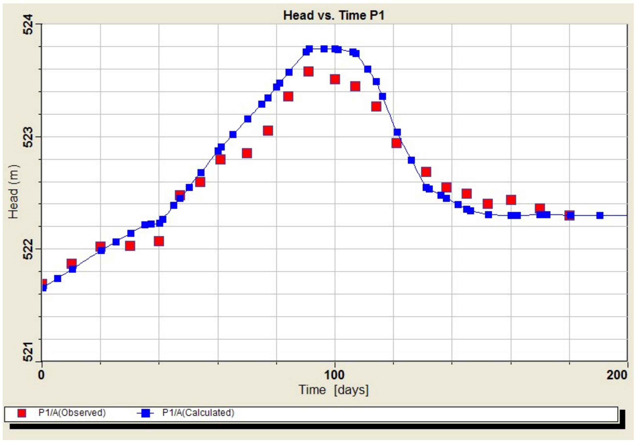
Figure 8.
Model calibration vs. observed groundwater head fluctuations in the W503K observation well, from April 2017 to November 2017.
Figure 8.
Model calibration vs. observed groundwater head fluctuations in the W503K observation well, from April 2017 to November 2017.
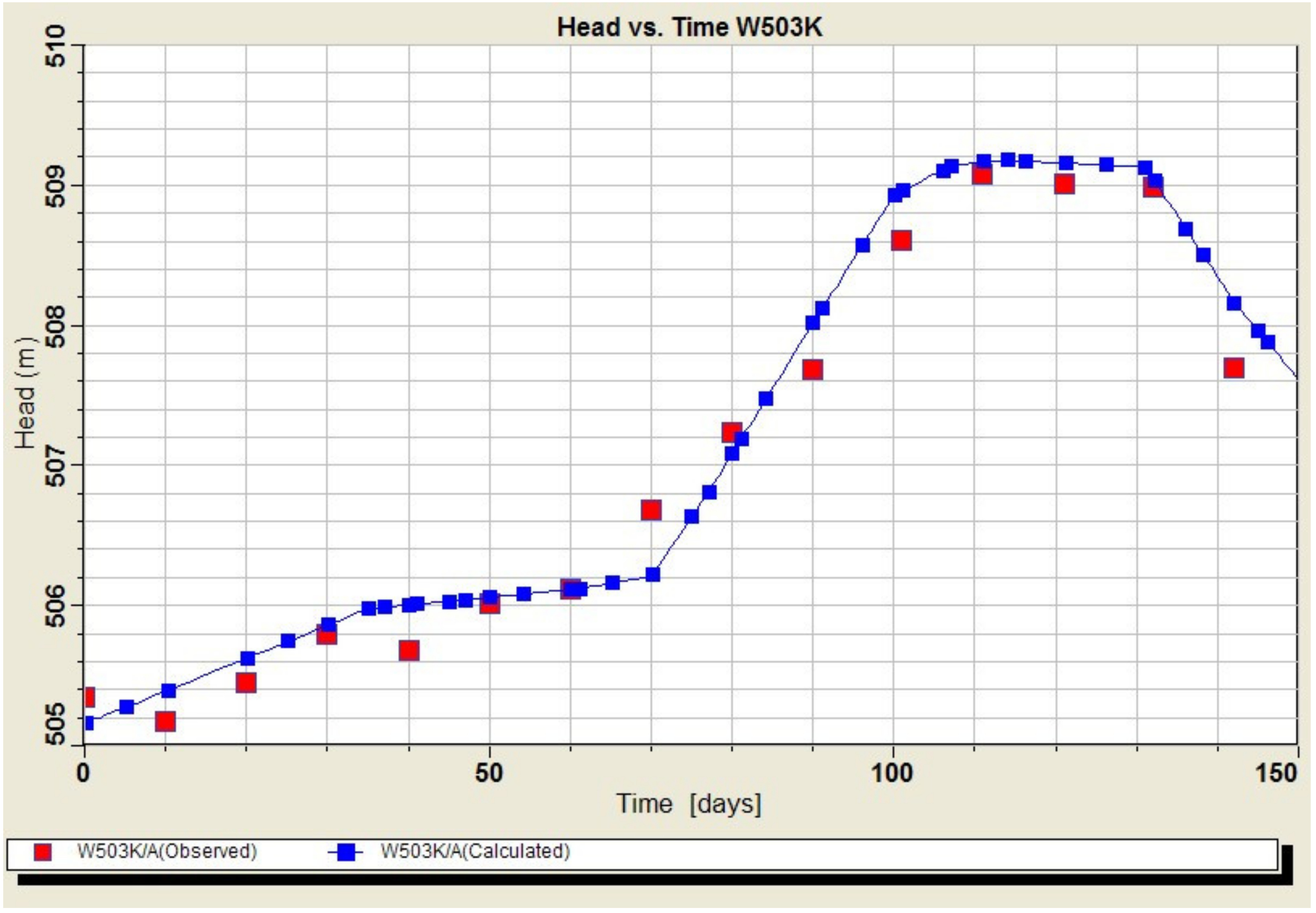
Figure 9.
Groundwater head contours and flow path, 15 July 2017.
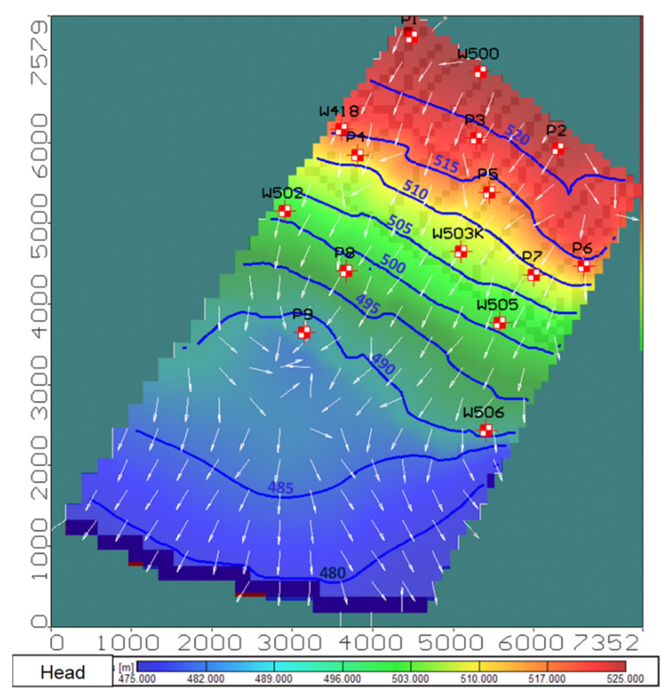
Figure 10.
Groundwater depth, 15 July 2017.
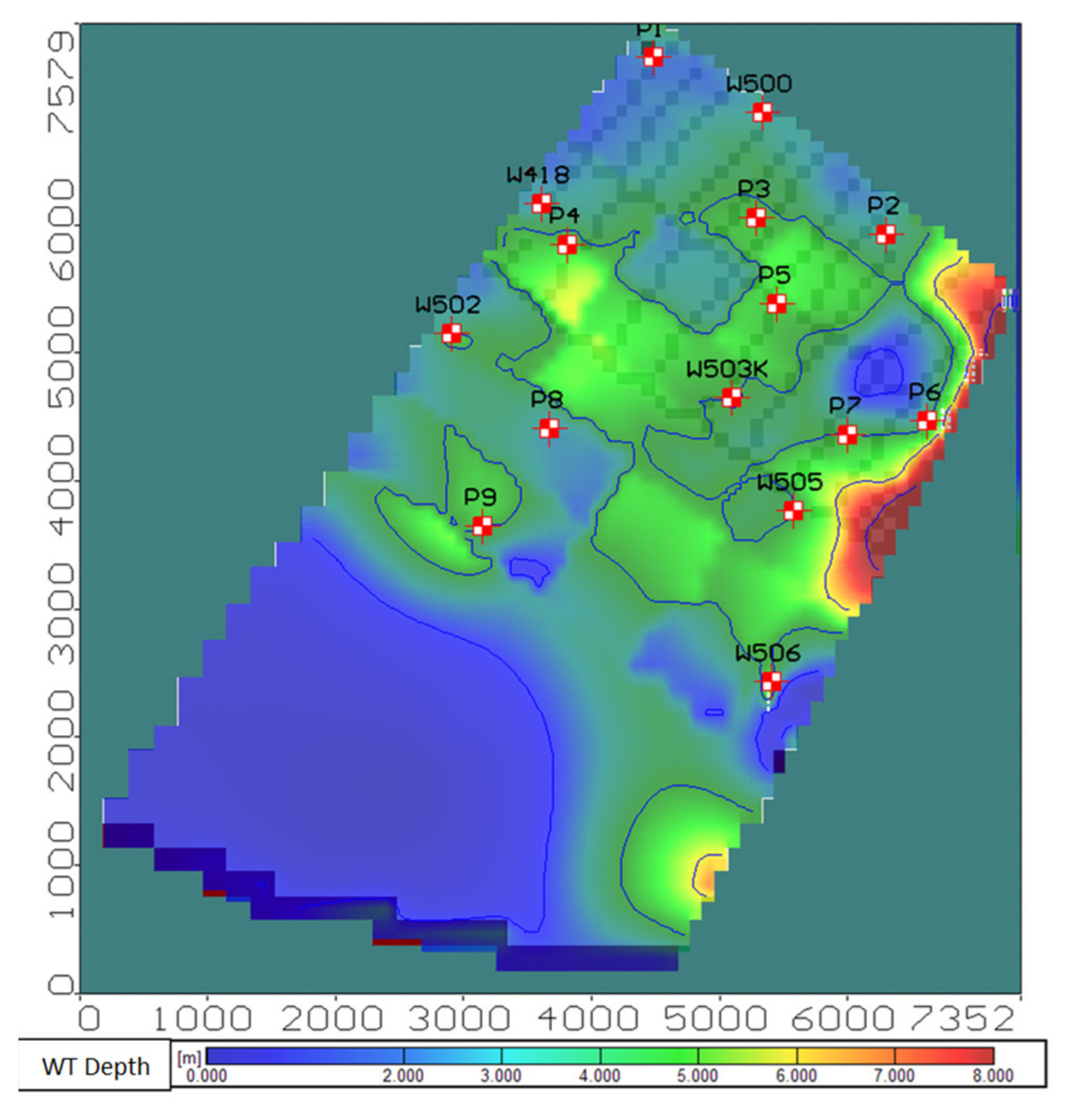
Figure 11.
Groundwater table depth for the end of the growing season (October): (A)—identification task; (B)—prediction task; 1—model blocks represent the additional recharge zone, instead of the “drain” boundary conditions.
Figure 11.
Groundwater table depth for the end of the growing season (October): (A)—identification task; (B)—prediction task; 1—model blocks represent the additional recharge zone, instead of the “drain” boundary conditions.
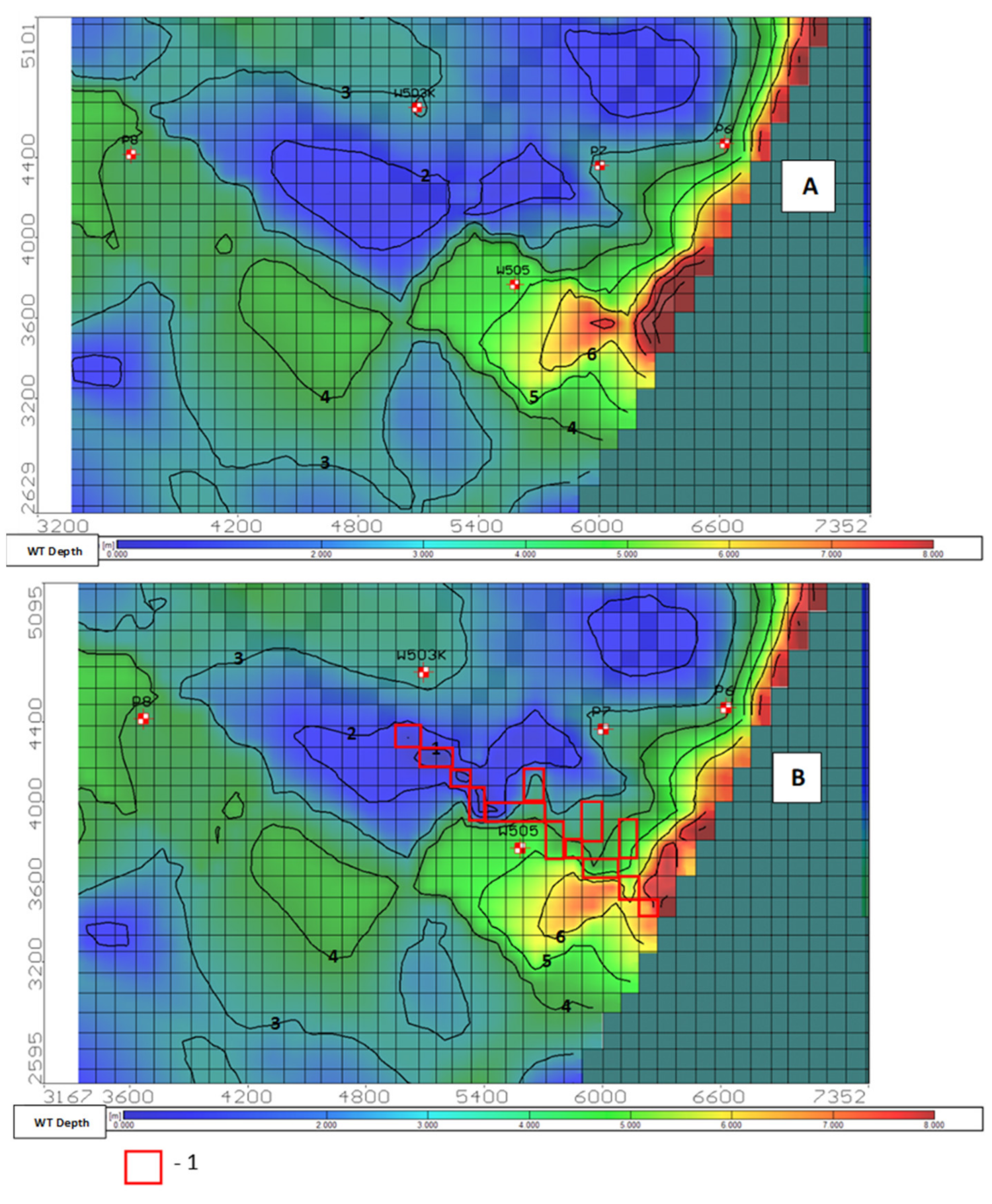
Figure 12.
Groundwater level fluctuation spatial and temporal variations.


Table 1.
Groundwater-flux balance at the Shengeldy experimental site was calculated for April, July, October, and November 2017. The results of the model calibration are in thousands of m3/day.
Table 1.
Groundwater-flux balance at the Shengeldy experimental site was calculated for April, July, October, and November 2017. The results of the model calibration are in thousands of m3/day.
| Date | 25-April | 15-July | 5-October | 15-November | |
|---|---|---|---|---|---|
| Input | Storage recharge | 16 | 10 | 111 | 76 |
| Infiltration from storage pond | 0.02 | 0.001 | 0.03 | 0 | |
| Infiltration of irrigation water and precipitation | 58.1 | 117 | 9.6 | 3.1 | |
| Total input | 74.5 | 126.6 | 120.9 | 78.7 | |
| Output | Storage discharge | 56.9 | 115.6 | 6.6 | 2.5 |
| Outflow to Kapshagai reservoir | 2.3 | 1.1 | 0.031 | −1 | |
| Areal discharge | 2.5 | 0 | 108.3 | 71.1 | |
| Evapotranspiration | 12 | 9.1 | 3.7 | 0.7 | |
| Drainage outflow | 0.9 | 0.6 | 1.6 | 0.4 | |
| Total output | 74.6 | 126.4 | 120.2 | 73.7 | |
| Input–output | −0.1 | 0.2 | 0.7 | 5 | |
Publisher’s Note: MDPI stays neutral with regard to jurisdictional claims in published maps and institutional affiliations. |
© 2021 by the authors. Licensee MDPI, Basel, Switzerland. This article is an open access article distributed under the terms and conditions of the Creative Commons Attribution (CC BY) license (https://creativecommons.org/licenses/by/4.0/).
Share and Cite
MDPI and ACS Style
Mirlas, V.; Makyzhanova, A.; Kulagin, V.; Kuldeev, E.; Anker, Y. An Integrated Aquifer Management Approach for Aridification-Affected Agricultural Area, Shengeldy-Kazakhstan. Water 2021, 13, 2357. https://doi.org/10.3390/w13172357
AMA Style
Mirlas V, Makyzhanova A, Kulagin V, Kuldeev E, Anker Y. An Integrated Aquifer Management Approach for Aridification-Affected Agricultural Area, Shengeldy-Kazakhstan. Water. 2021; 13(17):2357. https://doi.org/10.3390/w13172357
Chicago/Turabian StyleMirlas, Vladimir, Assyl Makyzhanova, Vitaly Kulagin, Erghan Kuldeev, and Yaakov Anker. 2021. "An Integrated Aquifer Management Approach for Aridification-Affected Agricultural Area, Shengeldy-Kazakhstan" Water 13, no. 17: 2357. https://doi.org/10.3390/w13172357
Note that from the first issue of 2016, this journal uses article numbers instead of page numbers. See further details here.