
Gas Pressure Dynamics in Small and Mid-Size Lakes
by
 and
and
Bertram Boehrer
1,*, 
Sylvia Jordan
2,
Peifang Leng
1,3,4,
Carolin Waldemer
1,
Cornelis Schwenk
1,5,
Michael Hupfer
2 and
Martin Schultze
1 1
Helmholtz-Centre for Environmental Research—UFZ, 39114 Magdeburg, Germany
2
Leibniz-Institute of Freshwater Ecology and Inland Fisheries—IGB, 12587 Berlin, Germany
3
Key Laboratory of Ecosystem Network Observation and Modeling, Institute of Geographic Sciences and Natural Resources Research, Chinese Academy of Sciences, Beijing 100101, China
4
College of Resources and Environment, University of Chinese Academy of Sciences, Beijing 100049, China
5
Institute for Environmental Physics, University Heidelberg, 69120 Heidelberg, Germany
*
Author to whom correspondence should be addressed.
Water 2021, 13(13), 1824; https://doi.org/10.3390/w13131824
Submission received: 1 June 2021
/
Revised: 14 June 2021
/
Accepted: 18 June 2021
/
Published: 30 June 2021
(This article belongs to the Special Issue Physical Processes in Lakes)
Abstract
:Dissolved gases produce a gas pressure. This gas pressure is the appropriate physical quantity for judging the possibility of bubble formation and hence it is central for understanding exchange of climate-relevant gases between (limnic) water and the atmosphere. The contribution of ebullition has widely been neglected in numerical simulations. We present measurements from six lacustrine waterbodies in Central Germany: including a natural lake, a drinking water reservoir, a mine pit lake, a sand excavation lake, a flooded quarry, and a small flooded lignite opencast, which has been heavily polluted. Seasonal changes of oxygen and temperature are complemented by numerical simulations of nitrogen and calculations of vapor pressure to quantify the contributions and their dynamics in lacustrine waters. In addition, accumulation of gases in monimolimnetic waters is demonstrated. We sum the partial pressures of the gases to yield a quantitative value for total gas pressure to reason which processes can force ebullition at which locations. In conclusion, only a small number of gases contribute decisively to gas pressure and hence can be crucial for bubble formation.
1. Introduction
Dissolved gases in aquatic systems have moved into the focus of limnological studies recently because of their central role in the carbon cycle and hence their relevance for the climate [1,2]. Lakes are known for the burial of organic material but also as sources of methane (CH4) and carbon dioxide (CO2). Lakes contribute decisively to fluxes of CH4 and CO2 into the atmosphere by both diffusive processes and ebullition [1]. CH4 is a highly potent greenhouse gas, i.e., a multiple of CO2 at equal concentrations [3]. The concentrations of both gases keep rising in the atmosphere. This fact emphasizes the need for elucidating the involvement of lakes and rivers in global carbon fluxes [4]. As a consequence, many recent studies have aimed at quantifying the fluxes from limnic waters into the atmosphere. In particular, reservoirs are known for releasing methane—especially in shallow or dry-falling areas. This fact may put the reputation of hydropower as green energy at stake at least in some cases [2,5].
Beyond their recognition as being climate-relevant, gases are central players in the ecology of limnic waters, especially oxygen (O2) for all breathing organisms and carbon dioxide (CO2) for photosynthetic organisms. Furthermore, dissolved gases that are conceived as less reactive such as nitrogen become relevant for nitrogen fixation when supply with inorganic nitrogen runs short (e.g., [6,7]).
Any dissolved gas produces a gas pressure. The contributions of all gases add up to the total gas pressure. Though not in wide use in limnology, total gas pressure is the proper physical quantity to judge proximity to spontaneous bubble formation and ebullition [8]. The ratios between partial pressures determine the composition of forming bubbles (e.g., [9,10]) and the exchange with the surrounding water while ascending through the waterbody to the surface [11]. In conclusion, putatively irrelevant gases have a decisive impact on the removal of ecologically relevant gases. Hence, gas pressure is central for quantifying gas fluxes to the atmosphere and for understanding ebullition.
Despite its relevance, gas pressure is not widely referred to in the limnological literature and appears nearly exclusively in connection with large-scale ebullition events—so-called limnic eruptions (e.g., [12]). Catastrophic events of spontaneous gas ebullition from deep waters (Lake Nyos and Lake Monoun—both in Cameroon, Africa) have cost the lives of many humans in single events [12,13,14,15]. Since then, a number of other lakes with gas pressures of concern have been reported in the literature (e.g., Lake Kivu: [16]) and assessed for the danger of limnic eruptions (Lake Kivu: [17], Guadiana pit Lake: [18]).
Distribution of gases in the water column and chemical reactions—most of them biologically mediated—change gas concentrations and hence affect gas pressure. However, a good overview of processes increasing gas pressure to the level of spontaneous ebullition is missing in the limnological literature as well as the physical limnology literature. The same accounts for the localization of these processes where gas pressure may be raised sufficiently. What limits the gas pressure and, if ebullition sets in, what controls the bubble composition and hence the removed or stripped gas? In conclusion, a closer competent view on the gas pressure in lakes with appropriate depictions is urgently needed to effectively impart the knowledge to the wider limnological community.
With this paper, we attempt to fill this gap. We present new data from six lakes in the German state of Saxony-Anhalt, including natural and artificial lakes reflecting the broad variety of limnic waters. Observations of extreme gas pressures in lakes are referred to in the discussion. Solubilities of the most relevant gases are listed in comparison. We demonstrate the contributions of the most relevant gases to gas pressure and complement the gas measurements with profiles from numerical model simulations to finally depict them together with their contributions to gas pressure. This gas pressure can be affected by chemical reactions (produced or removed) or temperature change. We demonstrate under which conditions total gas pressure can be raised to absolute pressure to finally result in bubble formation and ebullition.
2. Environmental Gases and Methods
2.1. Solubility of Gases
When a water surface gets into contact with the atmosphere, atmospheric gas flux goes into the water until an equilibrium concentration ci is reached, which is described by the Henry law:
where pi represents partial pressure in the gas phase (e.g., the atmosphere) and i is the marker for the different gases. Henry coefficients kH are specific for gases and depend on the temperature (and much weaker on other dissolved substances and pressure) (see Table 1 or [19]). The temperature effect is remarkable and the value roughly drops to half from 0 °C to 30 °C for many gases. A simplified quantitative description (e.g., Sander 2015) is
where has the dimension of (absolute) temperature and is generally determined empirically (also listed in Table 1; ΔsolH—dissolution enthalpy, general gas constant is the product of Avogadro number and Boltzmann constant).
If concentration is given in mol/L and partial pressure in bar, the Henry coefficient has the unit of (mol/L)/bar. However, both the concentration in the liquid phase as well as the partial pressure can be given in various units. Hence Henry coefficients can have differing units with accordingly differing values. A particularly interesting version of Henry coefficients results from replacing partial pressure pi with the concentration in the gas space cg,i, by applying the ideal gas law
As a consequence of having concentration on either side of Equation (1), the Henry coefficient does not possess a unit, and is commonly referred to as Bunsen coefficient (at 25 °C) or Ostwald coefficient (temperature dependent). This version of Henry coefficient relates concentration in the water directly to concentrations in the gas phase. Most common gases have a Bunsen coefficient in the range of 0.01 to 0.03 with the important exception of carbon dioxide, which has a Bunsen coefficient of the order of 1. In conclusion, most gases have concentrations of a factor 50 lower in solution than in the adjacent gas phase. Of the listed gases, only carbon dioxide is present at nearly the same concentration in equilibrated water as in air.
The conversion between units for concentrations is straightforward between mols and grams by multiplication by molar mass (in g/mol). However the conversion between molar units and other concentration units (e.g., molal units (mol/(kgH2O) or permille (or practical salinity units (psu) or g/(kgSample))) or partial pressures can be complex for a mixture of solutes [19,21,27].
A more accurate temperature fit compared to Equation (2) is achieved, when the Clausius-Clapeyron equation is solved and the result developed into a Taylor series, of which the exponent of the first three terms has the following form fitted with coefficients Ai (see also Supplementary Materials):
where we added a unit conversion factor u, as solubilities have traditionally been presented in a variation of different units.
Intuitively the Henry law is understood as a limited water volume in contact with an infinite atmosphere. However, the law also applies for a closed system with a limited air (or gas) space. Moreover in this case, partial pressures and concentrations are coupled: conditions inside the gas space are set by the concentrations in the water as used in headspace extractions for measurements of gas concentrations.
2.2. Gas Pressure, Saturation, Total Gas Pressure
By solving Henry’s law (Equation (1)) for pressure, we find that each dissolved volatile substance is connected to a gas pressure of its own, which is proportional to its concentration. Hence we can use the specific Henry coefficients to evaluate the gas pressures from concentration profiles of each gas. The temperature dependence of the Henry coefficient results in a temperature dependence of the gas pressure at given gas concentration (Equation (2), Table 1). However, in equilibrium between air and (e.g., surface) water, the dissolved gas in the water produces the same gas pressure as the partial pressure in the gas space. For a water surface at sea level and normal pressure, this amounts to 21% of 1013.25 mbar for oxygen: accordingly less for higher altitude, low air pressure and moist air.
Gas concentrations in the water can change due to sources and sinks. As a consequence, also gas pressures are affected. In addition, heating can raise gas pressures. The ratio between gas pressure and partial pressure in the adjacent air volume is defined as the saturation and usually given as a percentage with 100% representing equilibrium with dissolved gas and the adjacent air space. The conditions of partial pressures at the lake surface, which depend on air pressure and humidity at the time of measurement, function as the conventional reference, as instruments are usually calibrated on site. This reference, however, is variable in the range of few percent over the year due to changing weather conditions.
In the usual range of gas concentrations and pressures, gas pressures of all gases can be added to a total gas pressure: non-linearities and mutual interaction only play a role at extreme conditions: e.g., Lake Kivu [28]. A (hypothetical) bubble in the water column is subject to the gas pressure of the ambient water and it will eventually collapse, if local pressure pabs lies above total gas pressure ptdg [8,11]. As a consequence, the bubble formation limits the increase of total gas pressure to absolute pressure in natural waters (mainly hydrostatic and atmospheric pressure), which is a function of water depth. At greater depth, higher amounts of gases are soluble as a consequence.
2.3. Relevant Gases
Clearly, the number of detectable gases in natural water bodies goes far beyond those listed in Table 1. Unlisted gases may be of central ecological relevance and others are used for tracing water bodies, but only in very extreme cases, they may contribute considerably to the total gas pressure (e.g., [6,29,30,31]). We use the simple approximation of an exponential temperature dependence as this facilitates an easy intercomparison of solubility and temperature dependence. For many purposes, these approximations are sufficiently accurate, but calculations of high accuracy must use more sophisticated numerical approximations: for N2 and O2 [23], Ar [24], CH4 [25], and CO2 [26]. The deviation of the exponential fit and the more sophisticated approach lies within about 3% for temperature 10 to 35 °C; at lower temperatures deviation are even larger (see Supplementary Materials and Figure S1). The effect of dissolved solids on the Henry coefficient is small for freshwater (<3 g/L of dissolved solids) and quantifications are not available for salt compositions in inland waters (e.g., [28,32]) and hence has not been included in our evaluation.
In addition to the dissolved gases, water itself develops a vapor pressure which contributes to the total gas pressure as described by the Magnus equation. We follow the recommendation of Alduchov and Eskridge [33] and propose the simple formula for vapor pressure:
with temperature θ in °C.
This equation approximates the curve [34], which is recommended by the International Association of Properties of Water and Steam—IAPWS by better than 0.385% in the range 0 to 40 °C (see Supplementary Materials and Figure S2). Another good approximation (better than 0.006% even for temperatures beyond 40 °C) is proposed by Huang [35] (see Supplementary Materials).
Gas concentration in natural waters tend to equilibrate with the atmosphere while their surfaces are exposed to the atmosphere. However source and sink terms modify the concentrations. This can involve inflows, but also geochemical processes with many of them controlled by organisms. We included supporting information for a brief overview of the most important sources and sinks of the most important gases. Beyond this, we refer to textbooks on geochemistry of natural waters (such as [21,31]).
2.4. Simulations
To complement measurements for gases that have not been in field survey programmes, and to produce vertical profiles of good resolution, we implemented a simple one-dimensional model for a conservative gas, i.e., without sources and sinks in the water. We divided the water column into 48 equally spaced layers of d = 1 m thickness each. The simulations were run in MATLAB. Diffusion was implemented by exchanging half of each layer in steps of t = 30 days with neighboring layers to implement a turbulent diffusivity of the order k = d2/t = 4 × 10⁻⁷ m2/s. Equilibrium conditions were implemented for the gas for the entire epilimnion according to the measured water temperatures in spring and summer (as justified below in the results with measurements of oxygen in the epilimnion). As a result, we gained continuous and vertically coherent profiles for conservative gases.
3. Measurements
3.1. Investigated Lakes
The investigated lakes are located in Saxony-Anhalt, one federal state in Central Germany. This state has only few natural lakes as a consequence of its locations outside the area of the last glaciation. We present six lacustrine water bodies, including (1) a natural lake, (2) a drinking water reservoir, (3) one gravel pit lake, (4) one salt-affected mine pit lake and (5) one flooded quarry, and finally (6) one mine pit lake temporarily used as a dumping side (Figure 1). These water bodies are representative of the range of lacustrine waters in this area, which has been densely populated since the Middle Ages and hence intensively used for agriculture, forestry, settling, and exploitation of ore and salt deposits. Since the industrial revolution around 1870, it has also been heavily affected by traffic, lignite mining, and industrial production. Precipitation is generally low (around 550–600 mm per annum, except for the catchment of Rappbode Reservoir, where precipitation can reach up to 1700 mm per annum in the highest areas of the Harz mountains).
The lakes in detail:
- Rassnitzer See formed in the abandoned lignite mine Merseburg Ost 1b in the 1990s. Fresh and salty groundwater filled the void, resulting in a salinity-stratified water body, which does not overturn completely in winter. The final water level was reached by introducing freshwater from the nearby river Weisse Elster in 2002 [42,43,44,45].
- Barleber See is the residual of a gravel pit (gravel excavations took place at the beginning of the 1930s). As the local open air swimming facility of the city of Magdeburg, it is intensively used for recreation. Increasing nutrient concentrations led to heavy algal and cyanobacteria blooms and a restoration by alum treatment in 1986 [46,47]. A further use as recreational area required a second chemical treatment of the waters with poly-aluminum chloride from 9th July to 15th October 2019. Inflow and outflow exclusively happen through exchange with groundwater [48].
- Felsensee is a small lake, which formed in a former quarry. After stone production ceased, the quarry filled with groundwater. The water level has reached about 22 m. Higher conductivity groundwater inflows have turned the lake meromictic [49].
- Lake Vollert-Sued is a flooded opencast lignite mine. The pit was (until 1969) used to dispose of wastewater from lignite processing. There is no surficial inflow or outflow but exchange with groundwater balancing the evaporation deficit and causing groundwater contamination in the near vicinity of the lake [50,51]. Hence it is heavily affected through its history as a dumping site. The water has been treated in 1999 to reduce the unpleasant smell and the impact on animals in the area [52,53]. The lake has since been meromictic.
The first three lakes have been selected to demonstrate the oxygen dynamics under usual conditions, while the latter three were selected to demonstrate special features of gas production and accumulation in lakes.
3.2. Equipment
From most lakes, we could retrieve profiles of temperature and electrical conductivity as indicators of density stratification, as well as oxygen profiles at three times of the year: one profile in early spring before stratification set in, one in summer when surface temperatures were high, and one in autumn, when the cooling surface forced a deeper recirculation of the lake water. In the case of Felsensee, we only show measurements of one sampling date, as well as for Lake Vollert-Sued, where we include data from Horn et al. [53].
Following pieces of equipment were used:
- Arendsee: CTD profiles 2017: YSI 6600 V2, 2019: EXO2 from YSI, USA; optical oxygen sensor; CO2 and gas pressure measurement in a gas volume behind a permeable membrane; CO2 detection by IR spectrometry) CONTROS HydroC® CO2 from Kongsberg Maritime, Germany;
- Rappbode Reservoir: CTM90 from Sea & Sun Technology, Germany; optical oxygen sensor;
- Rassnitzer See: CTM90 from Sea & Sun Technology, Germany; optical oxygen sensor;
- Barleber See: CTM90 from Sea & Sun Technology, Germany; optical oxygen sensor;
- Felsensee: Ocean Seven 316 from Idronaut, Italy; amperometric oxygen sensor;
- Vollert Sued: CTD + O2: Ocean Seven 316 from Idronaut, Italy; amperometric oxygen sensor; gas pressure: (TDG-sensor pressure measurement in a gas filled permeable silicon tube) Hydrolab, USA; CH4, CO2 and N2: samples in GC thermal conductivity detector (see [53]).
4. Results
4.1. General Picture of Circulation and Atmospheric Recharge
Profiles with a multiparameter probe documented the stratification in the lakes Arendsee, Rappbode Reservoir, and (mine pit lake) Rassnitzer See (see Figure 1 and Table 2). During deep recirculation (profiles in March), the oxygen concentration was homogenized over the entire circulated water body (Figure 2, middle panel); the deep recirculation comprised the entire water body in holomictic Arendsee and Rappbode Reservoir. However, due to its meromictic character, the bottom 7 m of Rassnitzer See were not included in the deep recirculation. Oxygen levels remained at zero in the bottom waters. Profiles of oxygen saturation indicated that the entire circulated water body showed close to 100% saturation and hence was equilibrated with the atmosphere. Moreover, during summer and later in autumn, surface waters showed values close to 100% saturation.
During the stratification period, vertical exchange was largely reduced; hence local production and local depletion of oxygen could be observed in the water column. Both in Arendsee and Rappbode Reservoir, a reduction of oxygen concentrations could be measured: both lakes formed a metalimnetic oxygen minimum. This could possibly be attributed to the decomposition of organic material below the epilimnion, while the metalimnetic and hypolimnetic water remained disconnected from the supply with new oxygen from the atmosphere (see also [54,55] for Rappbode Reservoir; [56,57] for Arendsee).
On the contrary in Rassnitzer See, we saw a clear rise of oxygen saturation beyond 100% at depths of the thermocline and below. A small part of this could be attributed to primary production—assuming that sufficient light could enter deep enough to allow for photosynthesis: however, concentration profiles indicated that not much oxygen was added to the loading from spring deep recirculation. As a consequence, most of the rising saturation values had to be attributed to rising temperatures due to solar irradiation and turbulent diffusive heat transport from above beyond possible consumption and diffusive loses over the stratification period.
In general, we expected a very similar recharge and equilibration behavior of other gases, e.g., nitrogen and argon. Detailed documentations were not available as those concentrations are not particularly relevant for the ecology of a lake (see Section 2). However, contrary to mixing and recharge, we anticipated no relevant concentration changes over a stratification period due to geochemical reaction (as in the case of oxygen).
4.2. Complementing Gas Concentrations for Gas Pressure
We selected the 16th of August 2017 to produce a full set of profiles of relevant gases in Arendsee. Oxygen was measured with an optical sensor. It showed a minimum in the metalimnion (around 10 m depth), high values in the epilimnion, and lower values in the hypolimnion tending to zero toward the lake bed (Figure 3, left panel).
Carbon dioxide was low in the epilimnion due to the direct coupling to (the low) atmospheric concentrations. However, the deeper waters showed considerably higher concentrations. These concentrations corresponded to the missing O2 in the water column quite well, but they were not equal as the amount of produced CO2 from degrading biomass was not strictly tied to a stoichiometric value of 1, and some of the produced CO2 could be forwarded into bicarbonate (HCO3−) as a result of the carbonate equilibrium. Due to the strong depletion of oxygen in Arendsee, CO2 reached the same order of magnitude as O2.
Nitrogen (N2) is not as closely documented in lakes as oxygen. It is much less reactive and hence less relevant for ecological processes (see also discussion). Although, N2 is part of the nitrogen cycle, the supply probably never runs short. Usually, lake waters show N2 concentrations close to the atmospheric equilibrium even in meromictic lakes (e.g., [53]). As a consequence, N2 is often considered conservative, if no better information is available (e.g., [12]). Since also in our field programme nitrogen (N2) concentrations were not measured, we included simulated profiles from our simple 1D lake model assuming equilibration of the epilimnion with atmospheric concentrations of nitrogen and a turbulent diffusive exchange between layers (see above Section 2.4). As the deep water was recharged with N2 at a lower temperature (higher Henry coefficient), the hypolimnion showed higher concentrations than the epilimnion, which was equilibrated at summery temperatures. The transition through the metalimnion was smoothened by implementing diffusive transport. At all depths, N2 was obviously the gas with the highest concentration.
We also used the model for argon, where the conservative assumptions (no sources nor sinks) were satisfied even better. The profile looks nearly the same though concentrations were considerably lower due to the lower concentration in air compared to nitrogen; the numerical simulation profiles that demonstrate the vertical structure of a gas pressure profile.
Hydrogen sulphide has not been reported at noticeable concentrations in the open waters of Arendsee. Similarly, methane is removed during deep recirculation from this holomictic lake and cannot start to accumulate before oxygen is depleted. Measurements in the year 2019 [58] reconfirmed concentrations in the range of 100 nmol/L. Hence both gases could be neglected in the total gas pressure.
From the displayed concentration profiles, we calculated gas pressures by implementing a temperature-dependent Henry coefficient (Equation (1) solved for pi); temperatures were used from a CTD-probe profile. The calculation yielded the (by far) leading contribution from nitrogen N2; O2 provided a smaller contributions, while CO2—due to the high Henry coefficient—and argon (similar shape to N2, though at lower values)—due to low concentration—contributed only a much subordinate gas pressure. We also added vapor pressure of H2O, which was calculated as a function of temperature (Equation (6)) and hence was the third biggest gas pressure contribution in the epilimnion.
The gas pressures of all gases could be added to total gas pressure (Figure 3, right panel). We saw a local minimum in the metalimnion where oxygen had been depleted. Throughout the hypolimnion, gas pressures fell toward the lake bed as a consequence of reduced oxygen concentrations. Direct measurements of total gas pressure with the CO2 probe confirmed the structure of the total gas pressure profile well. Smaller deviations were attributed to the fact that the sensor was not optimized for total gas pressure but for CO2. The long response time might also have contributed to some additional error.
4.3. Elevated Gas Pressure Observations
Measurements in (the small gravel pit lake) Barleber See showed clearly elevated oxygen concentrations in the epilimnion during summer reaching a saturation of 140%, i.e., a gas pressure of 70 mbar above atmospheric (Figure 4, upper row). If N2 gas pressure was present at atmospheric gas pressure, then total gas pressure would have surmounted local pressure in the upper 70 cm of the water column and bubbles would be formed. Most probably bubbling had happened before and nitrogen had been stripped until total gas pressure lay below local pressure (observations of N2 to confirm this were not done).
In (the small quarry lake) Felsensee, a deep oxygen maximum was documented at 15 m depth in early August. The oxygen peak was accompanied by high values of chlorophyll-a fluorescence (Figure 4, middle row). Hence oxygen levels were attributed to photosynthetic activity of floating organisms at the upper edge of the monimolimnion. Obviously the organisms could profit from the chemical setting (nutrients or CO2) at this depth. Moreover, clearly below the epilimnion at depths 7–13 m, oxygen concentrations and gas pressures lay clearly above atmospheric oxygen pressure.
Finally gas concentrations in (the small polluted pit lake) Vollert-Sued were measured (data from Horn et al. [53]). In the monimolimnion, methane had accumulated and raised the gas pressure by more than 1 bar. Together with nitrogen, total gas pressure in the monimolimnion came into the range of the absolute pressure. Methane had been created by degradation of organic material in the sediment. Methane either diffused out of the sediment or formed bubbles which released part of their methane into the ambient (monimolimnetic) water while ascending through the water column. Bubbles could always be observed at the water surface.
5. Discussion
In most lacustrine waters, gas pressure is clearly dominated by nitrogen N2 and oxygen O2. While nitrogen is quite conservative and changes in N2 concentrations happen at a small rate, O2 is produced and used by aquatic organisms and hence O2 often shows a highly dynamic behavior in limnic systems. As a consequence, the oxygen contribution is the leading variable component of gas pressure in limnic waters. This is particularly visible in productive small lakes (e.g., Barleber See, Figure 4), as longer periods of weak winds allow a clear decoupling from the atmosphere. However, nitrogen always contributes a large portion to the total gas pressure and hence forms a large portion of the gas in bubbles.
In addition, gas pressure (and hence oxygen saturation) is affected by heating (e.g., solar irradiation into a density stratified layer, see upper hypolimnion of Rassnitzer See in Figure 2). Although concentrations may not change, the temperature dependence of the Henry coefficient will increase gas pressure when temperatures rise. Henry coefficients of N2, O2, Ar, and CH4 drop by a factor of about 2 over the limnologically interesting range from 0 °C to 30 °C. The temperature dependence of Henry coefficients of CO2 (and e.g., helium or neon) is noticeably different (see also noble gas thermometer [59]).
N2 concentrations can be retrieved from samples (as done for Lake Vollert-Sued ([53] Figure 4). However, such data sets have limited vertical resolution and limited vertical comparability as a consequence of possible error of chemical analysis between samples. Hence we decided to create continuous N2 profiles with a model approach from our understanding and assumption of conservative behavior. The resulting profile was realistic and included the typical features of the N2 profile (Figure 4). An increased N2 gas pressure in the metalimnion was the consequence of faster transport of heat (diffusive and by solar irradiation) than the N2 molecules.
Denitrification (forming N2 from inorganic nitrogen) and N2 fixation (forming organic nitrogen compounds from N2) happen at low rates in general. However a closer look at denitrification rates (e.g., [6]) reveals that even holomictic lakes may experience a production of N2 that may affect the N2 budget significantly over a stratification period (putatively in the range up to 10%). In monimolimnia, where more time would be available for accumulation (see below), the replenishment of nitrate is limited. On the other hand, nitrogen fixation probably can reduce the N2 budget and hence total gas pressure only in very special configurations. As a consequence, we encourage measurements of N2 when close investigation of total gas pressure in lakes are envisaged and accurate methods are available.
Furthermore in the range of 10 mbars, dissolved argon and vapor pressure contribute to gas pressure, which in general is in the order of 1 percent of total gas pressure. Hence, both gases are often neglected: in the case of argon, it is conveniently included in the nitrogen part (as gas chromatograph columns often do not separate Ar from O2 and N2, e.g., [9]). In the cold hypolimnetic water, the vapor pressure does not play an important role, but it does in warmer water: at 25 °C: water vapor pressure amounts to about 30 mbar and is the biggest contribution after N2 and O2 in the epilimnion (see Figure 3). As a consequence, moist samples in a head space contain about 3% of H2O, which can be found missing in the recovery rate of an accurate gas chromatography, if water vapor is not detected in separate (e.g., [32]).
Though the production and the removal of carbon dioxide is directly connected with the oxygen dynamics, its contribution to gas pressure is not relevant in holomictic lakes, as the Henry coefficient of CO2 is nearly two orders of magnitude larger. In addition, the involvement of the carbonate system extenuates the variability. For an accumulation that becomes relevant for gas pressure, long time periods must be provided (as in meromictic lakes) or a very strong source, e.g., from volcanic vents, has to supply gas [60,61].
Methane is usually not produced fast enough in the water column to contribute to gas pressure considerably; however conditions in the sediment are much more favorable [62]. Limnic sediments can provide a nearly inexhaustible amount of degradable organic material and anoxic conditions prevent the further oxidation of methane. Methane can diffuse out of sediment pores into the open water or alternatively form bubbles (see below), from which part of the methane is released into the water column while ascending to the lake surface.
5.1. Ebullition
The release of gases from the water body by bubbles is called ebullition. Bubbles can be formed and sustained, when gas pressure reaches absolute pressure (Figure 5; [8,63,64]). Such bubbles migrate toward the water surface due to their buoyancy. Mainly two gases are produced in natural waters by organisms to raise total gas pressure enough to force bubble formation: oxygen and methane.
In sunny conditions, primary production can form oxygen. Close to the surface, not much raising of the oxygen gas pressure is required to reach absolute pressure (e.g., Barleber See in Figure 4). However at greater depth, the gas pressure needs to be raised considerably before bubbles are form (e.g., Felsensee in Figure 4). As a consequence, elevated levels of oxygen can be seen before bubbles form. Deep chlorophyll maxima sustain primary production when they are exposed to favorable light conditions [6]. At a depth of 14 m in Felsensee (Figure 4) for example, an absolute pressure of 2.4 bar (1 bar atmospheric pressure plus 1.4 bar hydrostatic pressure) needs to be overcome. If gas pressure of N2 (and Ar) is at atmospheric equilibrium (i.e., 0.78 bar and 0.01 bar, respectively), the remainder to absolute pressure has to be accomplished by oxygen production until an O2 gas pressure of 2.4–0.79 bar = 1.61 bar is reached. 1.61 bar of oxygen gas pressure are commensurate with 750% of oxygen saturation (as 100% saturation mean 0.21 bar partial pressure of O2). In Felsensee, we detected close to 950 mbar (a saturation of nearly 450%) on the day of measurement. Whether this lake has ever reached the limit for ebullition has not been documented.
In general, the gas pressure of oxygen needs to be raised to
where the nitrogen gas pressure is the leading part in prest, and also gas pressures of argon and vapor are part of it (Figure 5).
Ebullition from macrophytes and algal mats on the lake bed has been documented much better: bubbles remain attached to the plants before they have grown enough to detach and ascend through the water column [65,66,67]. As long as a bubble remains attached to a plant, it is subject to gas exchange with the surrounding water [11]. Gases diffuse in and out, and—provided that enough time has been available—the gas composition (partial pressures) will reflect the gas pressure inside the water. The data presented from two small lakes [9] are compliant with this prediction.
The situation is very similar for methane bubbles. Methane is formed from biodegradation (see Supporting Information). This largely happens in the upper zone of the sediment. Methane can be accumulated in the pore space and finally form bubbles when total gas pressure reaches the absolute pressure (Figure 5). When the buoyancy is sufficient to escape from the sediment, methane bubbles enter the bottom water of the lake and start ascending through the water column [10,68,69].
Like oxygen bubbles, methane bubbles do not consist of pure methane, but contain mainly nitrogen and traces of other gases. As the bubbles also remove N2 from the pore water, this may be observable and even indicative of how much methane has been produced [10,70,71].
In conclusion, we could identify three possible zones of bubble release: (1) Close to the surface by oxygen release through primary production close to the water surface at roughly atmospheric composition Barleber See (Figure 4); (2) release of bubbles by accumulating oxygen in deep photosynthetically active areas (of phytoplankton of macrophytes: oxygen content is higher than atmospheric content ([9], see also Felsensee Figure 4); (3) Bubbles formed by methane production in the sediment mainly consist of methane and nitrogen ([10,53], see also Vollert-Sued Figure 4).
5.2. Other Mechanisms for Raising Gas Pressure and Releasing Gas Bubbles
At the surface, gas pressure could be raised by surface warming during the day. Warming releases bubbles of oxygen:nitrogen of 21:78. In Barleber See, oxygen saturation has clearly risen beyond 100% (see Figure 4, top row) and hence 0.21 bar. As the heating of the metalimnion is faster than the diffusive removal of nitrogen, a zone of high nitrogen pressure forms in the metalimnion (see Arendsee in Figure 3). This could contribute to forming bubbles in lakes where also oxygen is produced by photosynthesis at the same time. In addition, currently the most feared trigger mechanism for a catastrophic release of gas from Lake Kivu is submerged volcanic activity, bringing hot lava in contact with highly gas-charged deep water layers. Higher temperatures would correspond to lower Henry coefficients and hence to higher gas pressures. A chain reaction known as “limnic eruption” had been feared as a possible result.
Maeck et al. [72] showed that the release of methane from the river Saar/Mosel was triggered by surface waves originating from opening ship locks. The arriving wave trough lowered the pressure at the river bed, which resulted in bubbling. A similar connection exists with air pressure, wind, or water level changes [73,74,75]. When air pressure rises, Horn et al. [53] for example showed that ebullition decelerated while a falling air pressure increased the ebullition flux.
Water motions can impact the release of gases. Obviously if water parcels are moved vertically, they experience a lower hydrostatic pressure and release of gases can be triggered. In Lake Nyos, such an event following a land slide is the most commonly accepted trigger mechanism for the limnic eruption in 1986 [13].
Finally we want to mention that technical measures can raise gas pressure to values that even endanger aquatic life. To oppose oxygen depletion in hypolimnetic waters, aeration—i.e., introduction of air bubbles in the deep water can be considered. However the dissolution of bubbles under high pressure facilitates to raise gas pressure beyond atmospheric pressure, which can result in problems in particular for organisms that move vertically in the water column, such as fish (e.g., [76,77,78]). Excessively high gas pressures can be avoided by introducing only oxygen or—at least in part—by forcing the bubble plume to reach the water surface at the cost of money or changing the ecosystem. In addition, elevated gas pressures have been reported from reservoirs belonging to pumped storage plants.
5.3. Accumulation of Gases in Monimolimnia
Permanently stratified water bodies like meromictic lakes provide the preconditions for an accumulation of methane over long time scales at concentrations that eventually become relevant or even dominant for total gas pressure (e.g., [1,79,80]. Vollert-Sued is one example (Figure 3, bottom row), where degradable sediments have provided the material for methane formation. Methane and nitrogen form the gas pressure in the deep water. Famous other examples for a methane dominated gas pressure in monimolimnia are Lake Kivu, East Africa [60,81], and Lake Monticchio Piccolo, Italy [82].
Monimolimnia also accumulate carbon dioxide as an end product of biogeochemical degradation paths for organic matter. However, due to the good solubility of carbon dioxide, it takes a long time to form a CO2 gas pressure of concern only from organic degradation. The famous examples of extreme CO2 gas pressure: Lake Nyos, Lake Monoun (both in Cameroon), Kabuno Bay of Lake Kivu (in D.R. Congo), and main basin of Lake Kivu (in Rwanda and D.R. Congo) have a volcanic origin for the supply of CO2 [13,14,83]. In the special case of Guadiana Pit Lake (in Spain), acid rock drainage dissolved carbonate deposits in the underground and stored the formed CO2 in the monimolimnion [18,84].
The gas either originates from volcanic sources (e.g., Lake Nyos, Lake Monoun, Lake Kivu, Lake Monticchio Piccolo) or from geochemical interaction (Guadiana Pit Lake: [85]) or from biodegradation (Vollert-Sued pit lake). In all cases, either methane (Lake Kivu, Vollert-Sued, Monticchio Poccolo) or carbon dioxide (Nyos; Monoun; Guadiana Pit Lake: [18,86]) provide the leading contribution beyond the N2 background. The most prominent representative is Lake Kivu with its huge methane storage for commercial interest [16,28,32,83]. Especially high gas pressures of carbon dioxide are dangerous, as a sudden release can liberate an immense volume of gas to the atmosphere and threaten the lives of humans in the vicinity. Disastrous degassing happened at Lake Nyos and Lake Monoun in Cameroon in the 1980s [13,14,15].
Monimolimnia of meromictic lakes are shielded from direct exchange with the atmosphere. Water properties are renewed at a very slow rate. This yields ages of monimolimnia up to 800 years (Lake Kivu, Africa—Schmid et al. 2005) and more than 6000 years in the case of Salsvatn, Norway [87] or even 11,000 years in the case of Powell Lake, Canada [88,89]. Hence meromixis can provide a long time scale for the accumulation of solutes such as gases (see [79,90,91]).
It is clear that we may not have knowledge of all lakes with extreme gas pressure. Often H2S is reported as dangerous gas dissolved at high concentrations (kH = 0.1 mol/L/bar, TE = 2100 K [19]). Very high concentrations of sulphide (2.5 mmol/L) are found in Alatsee (Bavaria, Germany [92]). Depending on the pH, only part is present as dissolved H2S (Ks = 9.77 × 10⁻⁶) and hence contributes to gas pressure. At most, i.e., in acidic conditions (pH not reported), this corresponds to a gas pressure of 0.015 bar gas pressure at reported monimolimnion temperatures of 6 °C. Trapped ocean water could potentially produce about ten times as much sulphide from its dissolved sulphate, if losses by diffusion and precipitation would be small over the time period required for reducing the sulphate. We measured our highest sulphide concentrations (10 and 12 mmol/L) in the monimolimnion of Hufeisensee (Saxony-Anhalt, Germany, see also [93]), which corresponded to about 0.05 bar partial pressure of H2S (at measured pH = 6.8 and T = 6 °C). In conclusion, only in extreme cases, sulphide will provide a considerable contribution to the total gas pressure.
5.4. Final Remarks
From literature review and our own results, we confirm that in limnic waters only very few gases play an important role for gas pressure:
- 1.
- Nitrogen always contributes to gas pressure decisively and must be considered;
- 2.
- Oxygen from the atmosphere and from photosynthesis can contribute decisively to the gas pressure;
As far as documented, only under meromictic conditions in the deep anoxic waters (monimolimnion),
- 3.
- Methane (mainly from biodegradation or volcanic sources) or
- 4.
- Carbon dioxide (from external sources such as volcanic vents and geochemical reactions) can become an important or even the leading contribution to gas pressure.
In holomictic lakes, the gas pressure contribution of methane and carbon dioxide is small (usually even smaller than vapor and argon). At a smaller scale (gas pressure of tens of millibars), we can detect gas pressure of
- 5.
- Vapor pressure from water;
- 6.
- Argon from atmospheric sources.
All other gases play a much subordinate role. Other noble gases, chlorofluorocarbons, sulfurhexafluoride SF6 (e.g., [94,95]), and other gases may be used for tracing waters and dating the last intensive exchange with the atmosphere. It can be relevant to know their partial pressure to quantify the concentrations. However for total gas pressure, they do not play a role.
Bubbles in the open lake water can be created by photosynthetic oxygen production. This may be accomplished by submerged macrophytes and algal mats or planktonic algae closer to the surface. Additional heating may help forming bubbles as solubility of gases is temperature dependent. On the contrary, when bubbles form in the upper layer of the sediment, they originate from the decomposition of organic material where the produced methane is the leading component for raising the gas pressure. Biodegradation also produces carbon dioxide, but this contribution to gas pressure and hence for the release of bubbles is much lower due to the good solubility of carbon dioxide.
Nitrogen (N2) is produced by biogeochemical reactions, but rates usually are small in comparison to the N2 background. Hence nitrogen is rarely made responsible for forming bubbles. However, due to the high background of nitrogen gas pressure, it is very important for total gas pressure and hence contributes to a high portion of gas in the bubbles. The composition of the bubbles can be quantitatively calculated from partial pressures. In general, the required gas pressure of the produced gas (oxygen in open water or methane in the sediment) increases with depth (Equation (7)) and so does its portion in the bubble. Ascending bubbles are subject to exchange with the surrounding water (stripping).
Supplementary Materials
The following are available online at https://www.mdpi.com/article/10.3390/w13131824/s1, Figure S1: solubilities of the most relevant gases for gas pressure in lakes: left column: solubilities in mol/l/bar: simple exponential fits from Sander (2015) [19] in comparison to accurate parametrizations for N2 and O2 (Weiss 1970) [23], Ar (Jenkins et al. 2019) [24], CH4 (Wiesenburg and Guinasso 1979) [25] and CO2 (Weiss 1974) [26]. Right column: difference between approaches. Figure S2: Vapour pressure against temperature. Left panel: Huang (2018) [35] compared to the IAPWS recommended curve (Wagner and Pruss, 1993) [34]; right panel: Magnus equation compared to the recommendation of IAPWS (Wagner and Pruss, 1993) [34]. References [96,97,98,99,100,101,102,103,104,105,106,107,108,109,110,111,112,113,114,115,116,117,118,119,120,121,122,123,124,125,126,127,128,129] are cited in Supplementary Materials.
Author Contributions
Conceptualization, B.B. and C.W.; data curation, B.B., S.J., M.H. and M.S.; formal analysis, B.B., P.L., C.S. and M.S.; funding acquisition, M.H.; investigation, B.B., S.J., C.S. and M.S.; methodology, C.W.; resources, B.B., M.H. and M.S.; validation, B.B.; visualization, P.L. and C.S.; writing—original draft, B.B., S.J., P.L., C.W., C.S., M.H. and M.S.; writing—review and editing, B.B., C.W., C.S., M.H. and M.S. All authors have read and agreed to the published version of the manuscript.
Funding
The authors thank the city of Magdeburg for funding measurements on Barleber See, Deutsche Forschungsgemeinschaft—DFG for funding the project “newMOM” (ID: RI2040/4-1) and Talsperrenbetrieb Sachsen-Anhalt for supporting measurements on Rappbode Reservoir.
Institutional Review Board Statement
Not applicable.
Informed Consent Statement
Not applicable.
Data Availability Statement
Not applicable.
Acknowledgments
The authors would like to thank Karsten Rahn for measurements in Rassnitzer See, Rappbode Reservoir, Barleber See, and Vollert-Sued; Burkhard Kuehn for measurements in Barleber See and Thomas Hintze for the technical support at Arendsee. Many thanks to Matthias Koschorreck for comments on the manuscript.
Conflicts of Interest
The authors declare no conflict of interest.
References
- Bastviken, D.; Tranvik, L.J.; Downing, J.A.; Crill, P.; Enrich-Prast, A. Freshwater Methane Emissions Offset the Continental Carbon Sink. Science 2011, 331, 50. [Google Scholar] [CrossRef] [PubMed] [Green Version]
- Cole, J.J.; Prairie, Y.T.; Caraco, N.F.; McDowell, W.H.; Tranvik, L.J.; Striegl, R.G.; Duarte, C.M.; Kortelainen, P.; Downing, J.A.; Middelburg, J.J.; et al. Plumbing the global carbon cycle: Integrating inland waters into the terrestrial carbon budget. Ecosystems 2007, 10, 171–184. [Google Scholar]
- Myhre, G.; Shindell, D.; Bréon, F.; Collins, W.; Fuglestvedt, J.; Huang, J. Anthropogenic and natural radiative forcing. In Climate Change the Physical Science Basis. Contribution of Working Group I to the Fifth Assessment Report of the Intergovernmental Panel on Climate Change; Stocker, T.F., Qin., D., Plattner, G., Tignor, M., Allen, S.K., Boschung, J., Nauels, A., Xia, Y., Bex, V., Midgley, P.M., Eds.; Cambridge University Press: Cambridge, UK, 2013. [Google Scholar]
- Turner, A.J.; Frankenberg, C.; Wennberg, P.O.; Jacob, D.J. Ambiguity in the causes for decadal trends in atmospheric methane and hydroxyl. Proc. Nat. Acad. Sci. USA 2017, 114, 5367–5372. [Google Scholar] [CrossRef] [PubMed] [Green Version]
- Keller, P.S.; Catalán, N.; Von Schiller, D.; Grossart, H.-P.; Koschorreck, M.; Obrador, B.; Frassl, M.A.; Karakaya, N.; Barros, N.; Howitt, J.A.; et al. Global CO2 emissions from dry inland waters share common drivers across ecosystems. Nat. Commun. 2020, 11, 1–8. [Google Scholar] [CrossRef]
- Wetzel, R.G. Limnology: Lake and River Ecosystems, 3rd ed.; Academic Press: Cambridge, MA, USA, 2001. [Google Scholar]
- Higgins, S.N.; Paterson, M.J.; Hecky, R.E.; Schindler, D.W.; Venkiteswaran, J.J.; Findlay, D.L. Biological Nitrogen Fixation Prevents the Response of a Eutrophic Lake to Reduced Loading of Nitrogen: Evidence from a 46-Year Whole-Lake Experiment. Ecosystems 2018, 21, 1088–1100. [Google Scholar] [CrossRef]
- Miyake, Y. The Possibility and the Allowable Limit of Formation of Air Bubbles in the Sea. Pap. Meteorol. Geophys. 1951, 2, 95–101. [Google Scholar] [CrossRef]
- Koschorreck, M.; Hentschel, I.; Boehrer, B. Oxygen Ebullition from Lakes. Geophys. Res. Lett. 2017, 44, 9372–9378. [Google Scholar] [CrossRef]
- Langenegger, T.; Vachon, D.; Donis, D.; McGinnis, D.F. What the bubble knows: Lake methane dynamics revealed by sediment gas bubble composition. Limnol. Oceanogr. 2019, 64, 1526–1544. [Google Scholar] [CrossRef] [Green Version]
- McGinnis, D.F.; Greinert, J.; Artemov, Y.; Beaubien, S.E.; Wüest, A. Fate of rising methane bubbles in stratified waters: How much methane reaches the atmosphere? J. Geophys. Res. Space Phys. 2006, 111. [Google Scholar] [CrossRef] [Green Version]
- Halbwachs, M.; Sabroux, J.-C.; Grangeon, J.; Kayser, G.; Tochon-Danguy, J.-C.; Felix, A.; Beard, J.-C.; Villevieille, A.; Vitter, G.; Richon, P.; et al. Degassing the “killer lakes” Nyos and Monoun, Cameroon. Eos Transacti. Am. Geophys. 2004, 85, 281–285. [Google Scholar] [CrossRef] [Green Version]
- Sigurdsson, H.; Devine, J.; Tchua, F.; Presser, F.; Pringle, M.; Evans, W. Origin of the lethal gas burst from Lake Monoun, Cameroun. J. Volcanol. Geotherm. Res. 1987, 31, 1–16. [Google Scholar] [CrossRef]
- Kling, G.; Clark, M.A.; Wagner, G.N.; Compton, H.R.; Humphrey, A.M.; Devine, J.D.; Evans, W.C.; Lockwood, J.; Tuttle, M.L.; Koenigsberg, E.J. The 1986 Lake Nyos Gas Disaster in Cameroon, West Africa. Science 1987, 236, 169–175. [Google Scholar] [CrossRef] [Green Version]
- Freeth, S.J.; Kling, G.; Kusakabe, M.; Maley, J.; Tchoua, F.M.; Tietze, K.; Freeth, G.W.K.S.J. Conclusions from Lake Nyos disaster. Nature 1990, 348, 201. [Google Scholar] [CrossRef]
- Wüest, A.; Jarc, L.; Bürgmann, H.; Pasche, N.; Schmid, M. Methane Formation and Future Extraction in Lake Kivu. In Lake Kivu; Springer: Berlin/Heidelberg, Germany, 2012; pp. 165–180. [Google Scholar]
- Lorke, A.; Tietze, K.; Halbwachs, M.; Wüest, A. Response of Lake Kivu stratification to lava inflow and climate warming. Limnol. Oceanogr. 2004, 49, 778–783. [Google Scholar] [CrossRef] [Green Version]
- Boehrer, B.; Yusta, I.; Magin, K.; Sanchez-España, J. Quantifying, assessing and removing the extreme gas load from meromictic Guadiana pit lake, Southwest Spain. Sci. Total Environ. 2016, 563–564, 468–477. [Google Scholar] [CrossRef]
- Sander, R. Compilation of Henry’s law constants (version 4.0) for water as solvent. Atmosph. Chem. Phys. Discuss. 2015, 15, 4399–4981. [Google Scholar] [CrossRef] [Green Version]
- Roedel, W. Physik Unserer Umwelt: Die Atmosphäre; Springer: Heidelberg, Germany, 1992. [Google Scholar]
- Worch, E. Hydrochemistry. Basic Concepts and Exercises; De Gruyter: Berlin, Germany, 2015; (De Gruyter Graduate). [Google Scholar]
- Saunois, M.; Stavert, A.R.; Poulter, B.; Bousquet, P.; Canadell, J.G.; Jackson, R.B.; Raymond, P.A.; Dlugokencky, E.J.; Houweling, S.; Patra, P.K.; et al. The Global Methane Budget 2000–2017. Earth Syst. Sci. Data 2020, 12, 1561–1623. [Google Scholar] [CrossRef]
- Weiss, R. The solubility of nitrogen, oxygen and argon in water and seawater. Deep Sea Res. Oceanogr. Abstr. 1970, 17, 721–735. [Google Scholar] [CrossRef]
- Jenkins, W.; Lott, D.; Cahill, K. A determination of atmospheric helium, neon, argon, krypton, and xenon solubility concentrations in water and seawater. Mar. Chem. 2019, 211, 94–107. [Google Scholar] [CrossRef]
- Wiesenburg, D.A.; Guinasso, N.L. Equilibrium solubilities of methane, carbon monoxide and hydrogen in water and seawater. J. Chem. Eng. Data 1979, 24, 357–360. [Google Scholar] [CrossRef]
- Weiss, R. Carbon dioxide in water and seawater: The solubility of a non-ideal gas. Mar. Chem. 1974, 2, 203–215. [Google Scholar] [CrossRef]
- Dietz, S.; Lessmann, D.; Boehrer, B. Contribution of Solutes to Density Stratification in a Meromictic Lake (Waldsee/Germany). Mine Water Environ. 2012, 31, 129–137. [Google Scholar] [CrossRef]
- Bärenbold, F.; Boehrer, B.; Grilli, R.; Mugisha, A.; von Tümpling, W.; Umutoni, A.; Schmid, M. Updated dissolved gas concentrations in Lake Kivu from an intercomparison project. PLoS ONE 2020, 15, e0237836. [Google Scholar]
- Kipfer, R.; Aeschbach-Hertig, W.; Peeters, F.; Stute, M. Noble Gases in Lakes and Ground Waters. Rev. Miner. Geochem. 2002, 47, 615–700. [Google Scholar] [CrossRef]
- Christenson, B.; Tassi, F. Gases in Volcanic Lake Environments. In Advances in Volcanology; Springer: Berlin/Heidelberg, Germany, 2015; pp. 125–153. [Google Scholar]
- Worch, E. Wasser und Wasserinhaltsstoffe. Eine Einführung in die Hydrochemie. Wiesbaden, s.l.; Vieweg+Teubner Verlag: Berlin, Germany, 1997. [Google Scholar]
- Boehrer, B.; von Tuempling, W.; Mugisha, A.; Rogemont, C.; Umutoni, A. Reliable reference for the methane concentrations in Lake Kivu at the beginning of industrial exploitation. Hydrol. Earth Syst. Sci. 2019, 23, 4707–4716. [Google Scholar] [CrossRef] [Green Version]
- Alduchov, O.A.; Eskridge, R.E. Improved Magnus Form Approximation of Saturation Vapor Pressure. J. Appl. Meteorolog. 1996, 4, 601–609. [Google Scholar] [CrossRef]
- Wagner, W.; Pruss, A. International Equations for the Saturation Properties of Ordinary Water Substance. Revised According to the International Temperature Scale of Addendum to 1990. J. Phys. Chem. Ref. Data 1993, 16, 783–787. [Google Scholar] [CrossRef] [Green Version]
- Huang, J. A Simple Accurate Formula for Calculating Saturation Vapor Pressure of Water and Ice. J. Appl. Meteorol. Clim. 2018, 57, 1265–1272. [Google Scholar] [CrossRef]
- Hartmann, O.; Schönberg, G. Geologische Entwicklungsgeschichte und Untersuchungsergebnisse am Arendsee. Nachr. Arb. Unterwasserarchäologie 2009, 15, 58–64. [Google Scholar]
- Meinikmann, K.; Lewandowski, J.; Nützmann, G. Lacustrine groundwater discharge: Combined determination of volumes and spatial patterns. J. Hydrol. 2013, 502, 202–211. [Google Scholar] [CrossRef]
- Hannappel, S.; Köpp, C.; Rejman-Rasinska, E. Aufklärung der Ursachen zur Phosphorbelastung des oberflächennahen Grundwassers im hydraulischen Zustrom zum Arendsee in der Altmark. Hydrol. Wasserbewirtsch. 2020, 62, 25–38. [Google Scholar]
- Rinke, K.; Kuehn, B.; Bocaniov, S.; Wendt-Potthoff, K.; Büttner, O.; Tittel, J.; Schultze, M.; Herzsprung, P.; Rönicke, H.; Rink, K.; et al. Reservoirs as sentinels of catchments: The Rappbode Reservoir Observatory (Harz Mountains, Germany). Environ. Earth Sci. 2013, 69, 523–536. [Google Scholar] [CrossRef]
- Pöhlein, F.; Schultze, M.; Donner, J.; Dietze, M.; Wilhayn, S. Reaktionen eines zweistufigen Talsperrensystems auf Veränderungen des Stoffeintrags am Beispiel des Bodeswerks. Forum Hydrol. Wasserbewirtsch. 2004, 34, 137–144. [Google Scholar]
- Wentzky, V.C.; Tittel, J.; Jäger, C.G.; Rinke, K. Mechanisms preventing a decrease in phytoplankton biomass after phosphorus reductions in a German drinking water reservoir-results from more than 50 years of observation. Freshw. Biol. 2018, 63, 1063–1076. [Google Scholar] [CrossRef]
- Boehrer, B.; Heidenreich, H.; Schimmele, M.; Schultze, M. Numerical prognosis for salinity profiles of future lakes in the opencast mine Merseburg-Ost. Int. J. Salt Lake Res. 1998, 7, 235–260. [Google Scholar] [CrossRef]
- Heidenreich, H.; Boehrer, B.; Kater, R.; Hennig, G. Gekoppelte Modellierung geohydraulischer und limnophysikalischer Vorgänge in Tagebaurestseen und ihrer Umgebung. Grundwasser 1999, 4, 49–54. [Google Scholar] [CrossRef]
- Trettin, R.; Gläßer, W.; Lerche, I.; Seelig, U.; Treutler, H.-C. Flooding of lignite mines: Isotope variations and processes in a system influenced by saline groundwater. Isot. Environ. Health Stud. 2006, 42, 159–179. [Google Scholar] [CrossRef]
- Boehrer, B.; Kiwel, U.; Rahn, K.; Schultze, M. Chemocline erosion and its conservation by freshwater introduction to meromictic salt lakes. Limnology 2014, 44, 81–89. [Google Scholar] [CrossRef]
- Kong, X.; Seewald, M.; Dadi, T.; Friese, K.; Mi, C.; Boehrer, B.; Schultze, M.; Rinke, K.; Shatwell, T. Unravelling winter diatom blooms in temperate lakes using high frequency data and ecological modeling. Water Res. 2021, 190, 116681. [Google Scholar] [CrossRef]
- Rönicke, H.; Frassl, M.A.; Rinke, K.; Tittel, J.; Beyer, M.; Kormann, B.; Gohr, F.; Schultze, M. Suppression of bloom-forming colonial cyanobacteria by phosphate precipitation: A 30 years case study in Lake Barleber (Germany). Ecol. Eng. 2021, 162, 106171. [Google Scholar] [CrossRef]
- Hannappel, S.; Strom, A. Methode zur Ermittlung des Phosphoreintrags über das Grundwasser in den Barleber See bei Magdeburg. Korresp. Wasserwirtsch. 2020, 13, 24–30. [Google Scholar]
- Spott, D. Zum Chemismus der künstlichen Seen des Steinbruchgebiets zwischen Plötzky, Gommern und Pretzien. Nat. Nat. Heim. Bez. Halle Magdebg. 1967, 4, 43–53. [Google Scholar]
- Eccarius, B. Groundwater Monitoring and Isotope Investigation of Contaminated Wastewater from an Open Pit Mining Lake. Environ. Geosci. 1998, 5, 156–161. [Google Scholar] [CrossRef]
- Eccarius, B.; Christoph, G.; Ebhardt, G.; Glaser, W. Grundwassermodellierung zur Gefährdungsabschätzung eines phenolverseuchten Tagebaurestsees. Grundwasser 2001, 6, 61–70. [Google Scholar] [CrossRef]
- Stottmeister, U.; Kuschk, P.; Wiessner, A. Full-scale bioremediation and long-term monitoring of a phenolic wastewater disposal lake. Pure Appl. Chem. 2010, 82, 161–172. [Google Scholar] [CrossRef] [Green Version]
- Horn, C.; Metzler, P.; Ullrich, K.; Koschorreck, M.; Boehrer, B. Methane storage and ebullition in monimolimnetic waters of polluted mine pit lake Vollert-Sued, Germany. Sci. Total Environ. 2017, 584–585, 1–10. [Google Scholar] [CrossRef]
- Wentzky, V.C.; Frassl, M.A.; Rinke, K.; Boehrer, B. Metalimnetic oxygen minimum and the presence of Planktothrix rubescens in a low-nutrient drinking water reservoir. Water Res. 2019, 148, 208–218. [Google Scholar] [CrossRef]
- Mi, C.; Shatwell, T.; Ma, J.; Wentzky, V.C.; Boehrer, B.; Xu, Y.; Rinke, K. The formation of a metalimnetic oxygen minimum exemplifies how ecosystem dynamics shape biogeochemical processes: A modelling study. Water Res. 2020, 175, 115701. [Google Scholar] [CrossRef]
- Boehrer, B.; Schultze, M. Stratification of lakes. Rev. Geophys. 2008, 46. [Google Scholar] [CrossRef] [Green Version]
- Kreling, J.; Bravidor, J.; Engelhardt, C.; Hupfer, M.; Koschorreck, M.; Lorke, A. The importance of physical transport and oxygen consumption for the development of a metalimnetic oxygen minimum in a lake. Limnol. Oceanogr. 2016, 62, 348–363. [Google Scholar] [CrossRef]
- Xiao, S.; Liu, L.; Wang, W.; Lorke, A.; Woodhouse, J.; Grossart, H.-P. A Fast-Response Automated Gas Equilibrator (FaRAGE) for continuous in situ measurement of CH4 and CO2 dissolved in water. Hydrol. Earth Syst. Sci. 2002, 24, 3871–3880. [Google Scholar] [CrossRef]
- Aeschbach-Hertig, W.; Peeters, F.; Beyerle, U.; Kipfer, R. Interpretation of dissolved atmospheric noble gases in natural waters. Water Resour. Res. 1999, 35, 2779–2792. [Google Scholar] [CrossRef] [Green Version]
- Schmid, M.; Tietze, K.; Halbwachs, M.; Lorke, A.; McGinnis, D.F.; Wüest, A. How hazardous is the gas accumulation in Lake Kivu? Arguments for a risk assesment in light of the Nyiragongo volcano eruption of 2002. Acta Vulcanol. 2004, 14, 115–122. [Google Scholar]
- Avagyan, A.; Sahakyan, L.; Meliksetian, K.; Karakhanyan, A.; Lavrushin, V.; Atalyan, T.; Hovakimyan, H.; Avagyan, S.; Tozalakyan, P.; Shalaeva, E.; et al. New evidences of Holocene tectonic and volcanic activity of the western part of Lake Sevan (Armenia). Geol. Q. 2020, 64, 288–303. [Google Scholar] [CrossRef]
- Bastviken, D. Methan. In Encyclopedia of Inland Waters; Elsevier: Oxford, UK, 2009; pp. 783–805. [Google Scholar]
- Ramsey, W.L. Bubble growth from dissolved oxygen near the sea surface. Limnol. Oceanogr. 1962, 7, 1–7. [Google Scholar] [CrossRef]
- D’Aoust, B.G. Technical Note: Total Dissolved Gas Pressure (TDGP) Sensing in the Laboratory. Dissolut. Technol. 2007, 14, 38–41. [Google Scholar] [CrossRef]
- Long, M.H.; Sutherland, K.; Wankel, S.D.; Burdige, D.J.; Zimmerman, R.C. Ebullition of oxygen from seagrasses under supersaturated conditions. Limnol. Oceanogr. 2020, 65, 314–324. [Google Scholar] [CrossRef] [Green Version]
- Pedersen, O.; Colmer, T.D.; Esand-Jensen, K. Underwater Photosynthesis of Submerged Plants—Recent Advances and Methods. Front. Plant. Sci. 2013, 4, 140. [Google Scholar] [CrossRef] [Green Version]
- Mendoza-Lera, C.; Federlein, L.L.; Knie, M.; Mutz, M. The algal lift: Buoyancy-mediated sediment transport. Water Resourc. Res. 2016, 52, 108–118. [Google Scholar] [CrossRef] [Green Version]
- Boudreau, B.P. The physics of bubbles in surficial, soft, cohesive sediments. Mar. Pet. Geol. 2012, 38, 1–18. [Google Scholar] [CrossRef]
- Schmid, M.; Ostrovsky, I.; McGinnis, D.F. Role of gas ebullition in the methane budget of a deep subtropical lake: What can we learn from process-based modeling? Limnol. Oceanogr. 2017, 62, 2674–2698. [Google Scholar] [CrossRef] [Green Version]
- Reeburgh, W.S. Observations of gases in chesapeake bay sediments. Limnol. Oceanogr. 1969, 14, 368–375. [Google Scholar] [CrossRef] [Green Version]
- Brennwald, M.; Kipfer, R.; Imboden, D. Release of gas bubbles from lake sediment traced by noble gas isotopes in the sediment pore water. Earth Planet. Sci. Lett. 2005, 235, 31–44. [Google Scholar] [CrossRef]
- Maeck, A.; Hofmann, H.; Lorke, A. Pumping methane out of aquatic sediments—Ebullition forcing mechanisms in an impounded river. Biogeosciences 2014, 11, 2925–2938. [Google Scholar] [CrossRef] [Green Version]
- Joyce, J.; Jewell, P.W. Physical controls on methane ebullition from reservoirs and lakes. Environ. Eng. Geosci. 2003, 9, 167–178. [Google Scholar] [CrossRef] [Green Version]
- Chanton, J.P.; Martens, C.S.; Kelley, C.A. Gas transport from methane-saturated, tidal freshwater and wetland sediments. Limnol. Oceanogr. 1989, 34, 807–819. [Google Scholar] [CrossRef]
- Varadharajan, C.; Hemond, H.F. Time-series analysis of high-resolution ebullition fluxes from a stratified, freshwater lake. J. Geophys. Res. Space Phys. 2012, 117. [Google Scholar] [CrossRef]
- Gächter, R.; Wehrli, B. Ten years of artificial mixing and oxygenation: No effect on the internal phosphorus loading of two eutrophic lakes. Environ. Sci. Technol. 1998, 32, 3659–3665. [Google Scholar] [CrossRef]
- Bürgi, H.; Stadelmann, P. Change of phytoplankton composition and biodiversity in Lake Sempach before and during restoration. Hydrobiologia 2002, 469, 33–48. [Google Scholar] [CrossRef]
- Cooke, G.D.; Welch, E.B.; Peterson, S.A.; Nicols, S.L. Restoration and Management of Lakes and Reservoirs, 3rd ed.; CRC Press: Boca Raton, FL, USA, 2005. [Google Scholar]
- Boehrer, B.; Von Rohden, C.; Schultze, M. Physical Features of Meromictic Lakes: Stratification and Circulation. In Mediterranean-Type Ecosystems; Springer: Berlin/Heidelberg, Germany, 2017; pp. 15–34. [Google Scholar]
- Schultze, M.; Boehrer, B.; Wendt-Potthoff, K.; Katsev, S.; Brown, E.T. Chemical Setting and Biogeochemical Reactions in Meromictic Lakes. In Mediterranean-Type Ecosystems; Springer: Berlin/Heidelberg, Germany, 2017; pp. 35–59. [Google Scholar]
- Schmid, M.; Halbwachs, M.; Wehrli, B.; Wüest, A. Weak mixing in Lake Kivu: New insights indicate increasing risk of uncontrolled gas eruption. Geochem. Geophys. Geosyst. 2005, 6, Q07009. [Google Scholar] [CrossRef]
- Caracausi, A.; Nuccio, P.M.; Favara, R.; Nicolosi, M.; Paternoster, M. Gas hazard assessment at the Monticchio crater lakes of Mt. Vulture, a volcano in Southern Italy. Terra Nova 2009, 21, 83–87. [Google Scholar] [CrossRef]
- Tietze, K.; Geyh, M.; Müller, H.; Schröder, L.; Stahl, W.; Wehner, H. The genesis of the methane in Lake Kivu (Central Africa). Acta Diabetol. 1980, 69, 452–472. [Google Scholar] [CrossRef]
- Sánchez-España, J.; Boehrer, B.; Yusta, I. Extreme carbon dioxide concentrations in acidic pit lakes provoked by water/rock interaction. Environ. Sci. Technol. 2014, 48, 4273–4281. [Google Scholar] [CrossRef]
- Sánchez-España, J.; Falagán, C.; Ayala, D.; Wendt-Potthoff, K. Adaptation of Coccomyxa sp. to extremely low light conditions causes deep chlorophyll and oxygen maxima in acidic pit lakes. Microorganisms 2020, 8, 1218. [Google Scholar] [CrossRef] [PubMed]
- Sánchez-España, J.; Yusta, I.; Boehrer, B. Degassing Pit Lakes: Technical Issues and Lessons Learnt from the HERCO2 Project in the Guadiana Open Pit (Herrerías Mine, SW Spain). Mine Water Environ. 2020, 39, 517–534. [Google Scholar] [CrossRef]
- Strøm, K.; Str, K. A Lake with Trapped Sea-Water? Nat. Cell Biol. 1957, 180, 982–983. [Google Scholar] [CrossRef]
- Williams, P.M.; Mathews, W.H.; Pickard, G.L. A Lake in British Columbia containing Old Sea-Water. Nat. Cell Biol. 1961, 191, 830–832. [Google Scholar] [CrossRef]
- Sanderson, B.; Perry, K.; Pedersen, T. Vertical diffusion in meromictic Powell Lake, British Columbia. J. Geophys. Res. Space Phys. 1986, 91, 7647. [Google Scholar] [CrossRef]
- Gulati, R.D.; Zadereev, E.S.; Degermendzhi, A.G. Ecology of meromictic lakes. In Ecological Studies 228; Springer: Berlin/Heidelberg, Germany, 2017. [Google Scholar]
- Zadereev, E.S.; Gulati, R.D.; Camacho, A. Biological and Ecological Features, Trophic Structure and Energy Flow in Meromictic Lakes. In Mediterranean-Type Ecosystems; Springer: Berlin/Heidelberg, Germany, 2017; pp. 61–86. [Google Scholar]
- Oikomonou, A.; Filker, S.; Breiner, H.-W.; Stoeck, T. Protistan diversity in a permanently stratified meromictic lake (Lake Alatsee, SW Germany). Environ. Microbiol. 2015, 17, 2144–2157. [Google Scholar] [CrossRef]
- Nitzsche, H.M. Chemical and Isotope Investigations in Dissolved Gases of a Meromictic Residual Lake. Isotop. Environ. Health Stud. 1999, 35, 63–73. [Google Scholar] [CrossRef]
- Maiss, M.; Ilmberger, J.; Münnich, K.O. Vertical mixing in Überlingersee (Lake Constance) traced by SF 6 and heat. Aquat. Sci. 1994, 56, 329–346. [Google Scholar] [CrossRef]
- Von Rohden, C.; Ilmberger, J.; Boehrer, B. Assessing groundwater coupling and vertical exchange in a meromictic mining lake with an SF6-tracer experiment. J. Hydrol. 2009, 372, 102–108. [Google Scholar] [CrossRef]
- Aeschbach-Hertig, W.; Kipfer, R.; Hofer, M.; Imboden, D.; Wieler, R.; Signer, P. Quantification of gas fluxes from the subcontinental mantle: The example of Laacher See, a maar lake in Germany. Geochim. Cosmochim. Acta 1996, 60, 31–41. [Google Scholar] [CrossRef]
- Bärenbold, F.; Schmid, M.; Brennwald, M.S.; Kipfer, R. Missing atmospheric noble gases in a large, tropical lake: The case of Lake Kivu, East-Africa. Chem. Geol. 2020, 532, 119374. [Google Scholar] [CrossRef]
- Baulch, H.M.; Dillon, P.J.; Maranger, R.; Schiff, S.L. Diffusive and ebullitive transport of methane and nitrous oxide from streams: Are bubble-mediated fluxes important? J. Geophys. Res. Space Phys. 2011, 116. [Google Scholar] [CrossRef]
- Bräuer, K.; Geissler, W.H.; Kämpf, H.; Niedermann, S.; Rman, N. Helium and carbon isotope signatures of gas exhala-tions in the westernmost part of the Pannonian Basin (SE Austria/NE Slovenia): Evidence for active lithospheric mantle de-gassing. Chem. Geol. 2016, 422, 60–70. [Google Scholar] [CrossRef]
- Burton, M.R.; Sawyer, G.M.; Granieri, D. Deep Carbon Emissions from Volcanoes. Rev. Miner. Geochem. 2013, 75, 323–354. [Google Scholar] [CrossRef] [Green Version]
- Chambers, L.; Gooddy, D.; Binley, A. Use and application of CFC-11, CFC-12, CFC-113 and SF6 as environmental tracers of groundwater residence time: A review. Geosci. Front. 2019, 10, 1643–1652. [Google Scholar] [CrossRef]
- Emerson, S.; Quay, P.D.; Stump, C.; Wilbur, D.; Schudlich, R. Chemical tracers of productivity and respiration in the subtropical Pacific Ocean. J. Geophys. Res. Space Phys. 1995, 100, 15873. [Google Scholar] [CrossRef]
- Etiope, G.; Klusman, R. Microseepage in drylands: Flux and implications in the global atmospheric source/sink budget of methane. Glob. Planet. Chang. 2010, 72, 265–274. [Google Scholar] [CrossRef]
- Etiope, G.; Lollar, B.S. Abiotic methane on Earth. Rev. Geophys. 2013, 51, 276–299. [Google Scholar] [CrossRef]
- Etiope, G.; Ciotoli, G.; Schwietzke, S.; Schoell, M. Gridded maps of geological methane emissions and their isotopic signature. Earth Syst. Sci. Data 2019, 11, 1–22. [Google Scholar] [CrossRef] [Green Version]
- Frondini, F.; Cardellini, C.; Caliro, S.; Beddini, G.; Rosiello, A.; Chiodini, G. Measuring and interpreting CO2 fluxes at regional scale: The case of the Appennines, Italy. J. Geol. Soc. 2019, 176, 408–416. [Google Scholar] [CrossRef] [Green Version]
- Giggenbach, W.E.; Sano, Y.; Schmincke, H.U. CO2-rich gases from Lakes Nyos and Monoun, Cameroon; Laacher See, Germany; Dieng, Indonesia, and Mt. Gambier, Australia—Variations on a common theme. J. Volcanol. Geotherm. Res. 1991, 45, 311–323. [Google Scholar] [CrossRef]
- Guidotti, T.L. Hydrogen Sulphide. Occup. Med. 1996, 46, 367–371. [Google Scholar] [CrossRef] [PubMed] [Green Version]
- Hamersley, M.R.; Turk, K.; Leinweber, A.; Gruber, N.; Zehr, J.; Gunderson, T.; Capone, D. Nitrogen fixation within the water column associated with two hypoxic basins in the Southern California Bight. Aquat. Microb. Ecol. 2011, 63, 193–205. [Google Scholar] [CrossRef] [Green Version]
- Hamersley, M.R.; Woebken, D.; Boehrer, B.; Schultze, M.; Lavik, G.; Kuypers, M.M. Water column anammox and denitrification in a temperate permanently stratified lake (Lake Rassnitzer, Germany). Syst. Appl. Microbiol. 2009, 32, 571–582. [Google Scholar] [CrossRef] [PubMed]
- Hunt, J.A.; Zafu, A.; Mather, T.A.; Pyle, D.M.; Barry, P. Spatially Variable CO2 Degassing in the Main Ethiopian Rift: Implications for Magma Storage, Volatile Transport, and Rift-Related Emissions. Geochem. Geophys. Geosystems 2017, 18, 3714–3737. [Google Scholar] [CrossRef]
- Kämpf, H.; Bräuer, K.; Schumann, J.; Hahne, K.; Strauch, G. CO2 discharge in an active, non-volcanic continental rift area (Czech Republic): Characterisation (δ13C, 3He/4He) and quantification of diffuse and vent CO2 emissions. Chem. Geol. 2013, 339, 71–83. [Google Scholar] [CrossRef]
- Kelemen, P.B.; Manning, C.E. Reevaluating carbon fluxes in subduction zones, what goes down, mostly comes up. Proc. Natl. Acad. Sci. USA 2015, 112, E3997–E4006. [Google Scholar] [CrossRef] [Green Version]
- Kerrick, D.M. Present and past nonanthropogenic CO2 degassing from the solid earth. Rev. Geophys. 2001, 39, 565–585. [Google Scholar] [CrossRef]
- Koutsoyiannis, D. Clausius–Clapeyron equation and saturation vapour pressure: Simple theory reconciled with practice. Eur. J. Phys. 2012, 33, 295–305. [Google Scholar] [CrossRef]
- Lee, S.; Kang, N.; Park, M.; Hwang, J.Y.; Yun, S.H.; Jeong, H.Y. A review on volcanic gas compositions related to volcanic activities and non-volcanological effects. Geosci. J. 2018, 22, 183–197. [Google Scholar] [CrossRef]
- Lewis, A.E. Review of metal sulphide precipitation. Hydrometallurgy 2010, 104, 222–234. [Google Scholar] [CrossRef]
- Madigan, M.T.; Martinko, J.M.; Stahl, D.A.; Clark, D.P. Brock Mikrobiologie, 13th ed.; Pearson: Munich, Germany, 2013. [Google Scholar]
- Macpherson, G. CO2 distribution in groundwater and the impact of groundwater extraction on the global C cycle. Chem. Geol. 2009, 264, 328–336. [Google Scholar] [CrossRef]
- Moreira, S.; Schultze, M.; Rahn, K.; Boehrer, B. A practical approach to lake water density from electrical conductivity and temperature. Hydrol. Earth Syst. Sci. 2016, 20, 2975–2986. [Google Scholar] [CrossRef] [Green Version]
- Van de Graaf, A.A.; Mulder, A.; de Bruijn, P.; Jetten, M.S.; Robertson, L.A.; Kuenen, J.G. Anaerobic ammonium oxidation discovered in a denitri-fying fluidized bed reactor. FEMS Microbiol. Ecol. 1995, 16, 177–183. [Google Scholar] [CrossRef]
- Poissant, L.; Constant, P.; Pilote, M.; Canário, J.; O’Driscoll, N.; Ridal, J.; Lean, D. The ebullition of hydrogen, carbon monoxide, methane, carbon dioxide and total gaseous mercury from the Cornwall Area of Concern. Sci. Total Environ. 2007, 381, 256–262. [Google Scholar] [CrossRef]
- Press, F.; Siever, R.; Jordan, T.H.; Grontzinger, J. Understanding Earth, 4th ed.; W. H. Freeman & Co.: New York, NY, USA, 2003. [Google Scholar]
- Raymond, P.A.; Hartmann, J.; Lauerwald, R.; Sobek, S.; McDonald, C.; Hoover, M.; Butman, D.; Striegl, R.; Mayorga, E.; Humborg, C.; et al. Global carbon dioxide emissions from inland waters. Nature 2013, 503, 355–359. [Google Scholar] [CrossRef] [Green Version]
- Ross, K.A.; Gashugi, E.; Gafasi, A.; Wüest, A.; Schmid, M. Characterisation of the Subaquatic Groundwater Discharge That Maintains the Permanent Stratification within Lake Kivu; East Africa. PLoS ONE 2015, 10, e0121217. [Google Scholar] [CrossRef]
- Schink, B. Energetics of syntrophic cooperation in methanogenic degradation. Microbiol. Mol. Biol. Rev. 1997, 61, 262–280. [Google Scholar] [CrossRef] [PubMed] [Green Version]
- Schink, B. Microbially driven redox reactions in anoxic environments: Pathways, energetics, and biochemical conse-quences. Eng. Life Sci. 2006, 6, 228–233. [Google Scholar] [CrossRef] [Green Version]
- Sobolewski, A. Metal species indicate the potential of constructed wetlands for long-term treatment of metal mine drainage. Ecol. Eng. 1996, 6, 259–271. [Google Scholar] [CrossRef]
- Stumm, W.; Morgan, J.J. Aquatic Chemistry, 3rd ed.; John Wiley and Sons: New York, NY, USA, 1996. [Google Scholar]
Figure 1.
Location of investigated lakes; depth contour maps Arendsee, Rappbode Reservoir, Rassnitzer See, Barleber See, Vollert-Sued, Felsensee.
Figure 1.
Location of investigated lakes; depth contour maps Arendsee, Rappbode Reservoir, Rassnitzer See, Barleber See, Vollert-Sued, Felsensee.
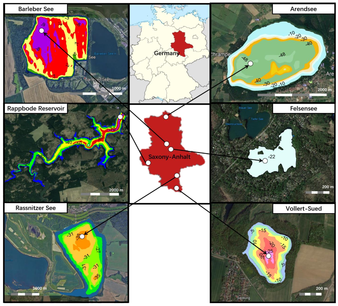
Figure 2.
Profiles measured in Arendsee, Rappbode Reservoir, Rassnitzer See (all located in Saxony-Anhalt, Germany) on three sampling dates (green: spring, red; summer, black: autumn) in 2019: temperature, electrical conductivity, dissolved oxygen concentration, oxygen gas pressure (dotted line: atmospheric gas pressure at lake surface), oxygen saturation (dotted line: 100% saturation).
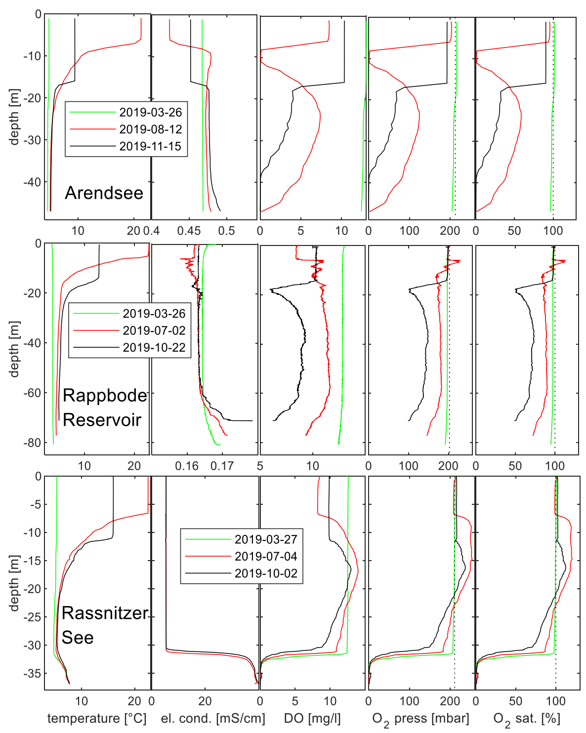
Figure 3.
Left panel: concentration of gases in Arendsee on 16 August 2017: right panel: Gas pressures. Oxygen and carbon dioxide gas pressures were measured, while nitrogen and argon were modelled (see text), whereas vapor pressure was calculated from a temperature profile; total gas pressure was calculated from adding the partial pressures of displayed volatile substances and drawn with directly measured total gas pressure from the CO2 probe (symbols). Broken lines (for epilimnion values of N2 and total gas pressure) do not represent the real situation.

Figure 4.
Profiles from the lakes: Barleber See, Felsensee, Vollert-Sued showing measured profiles of temperature, el. conductivity, gas concentrations, gas pressures (dotted line: atmospheric O2 partial pressure above lake surface) and oxygen saturation (dotted line: 100% saturation). Felsensee O2 data have been compensated for 6.5 s response time of the amperometric sensor from raw data. Vollert-Sued: psum: sum of calculated gas pressures; ptdg: directly measured total gas pressure; pabs: absolute pressure calculated as atmospheric plus hydrostatic.

Figure 5.
Gas pressure against depth in an idealized lake, gas pressure of argon is included in the N2 value, gas pressures of other gases and water vapor pressure are neglected.
Figure 5.
Gas pressure against depth in an idealized lake, gas pressure of argon is included in the N2 value, gas pressures of other gases and water vapor pressure are neglected.
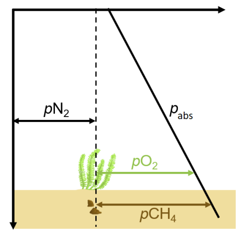

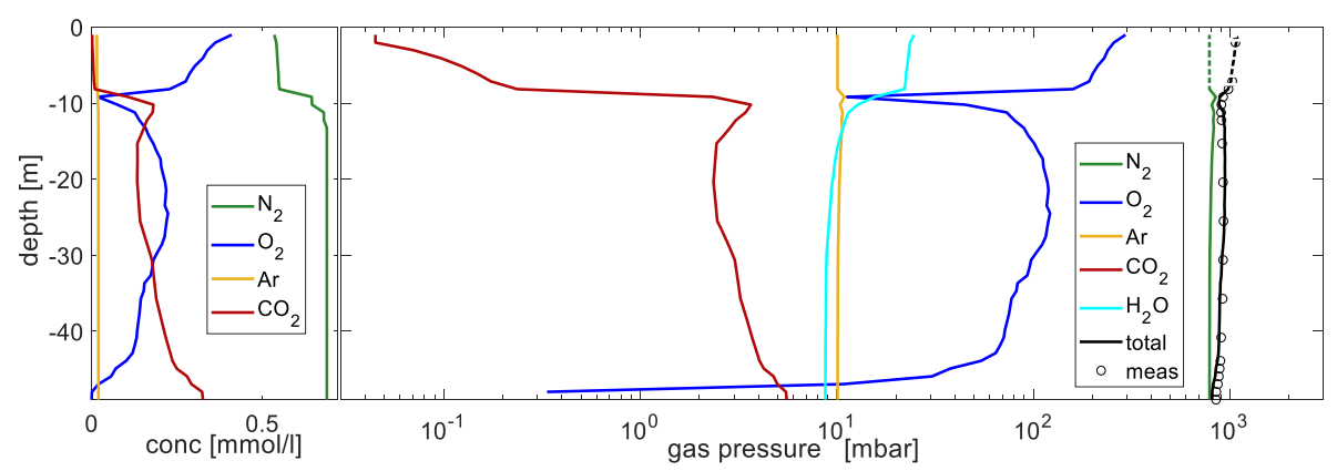
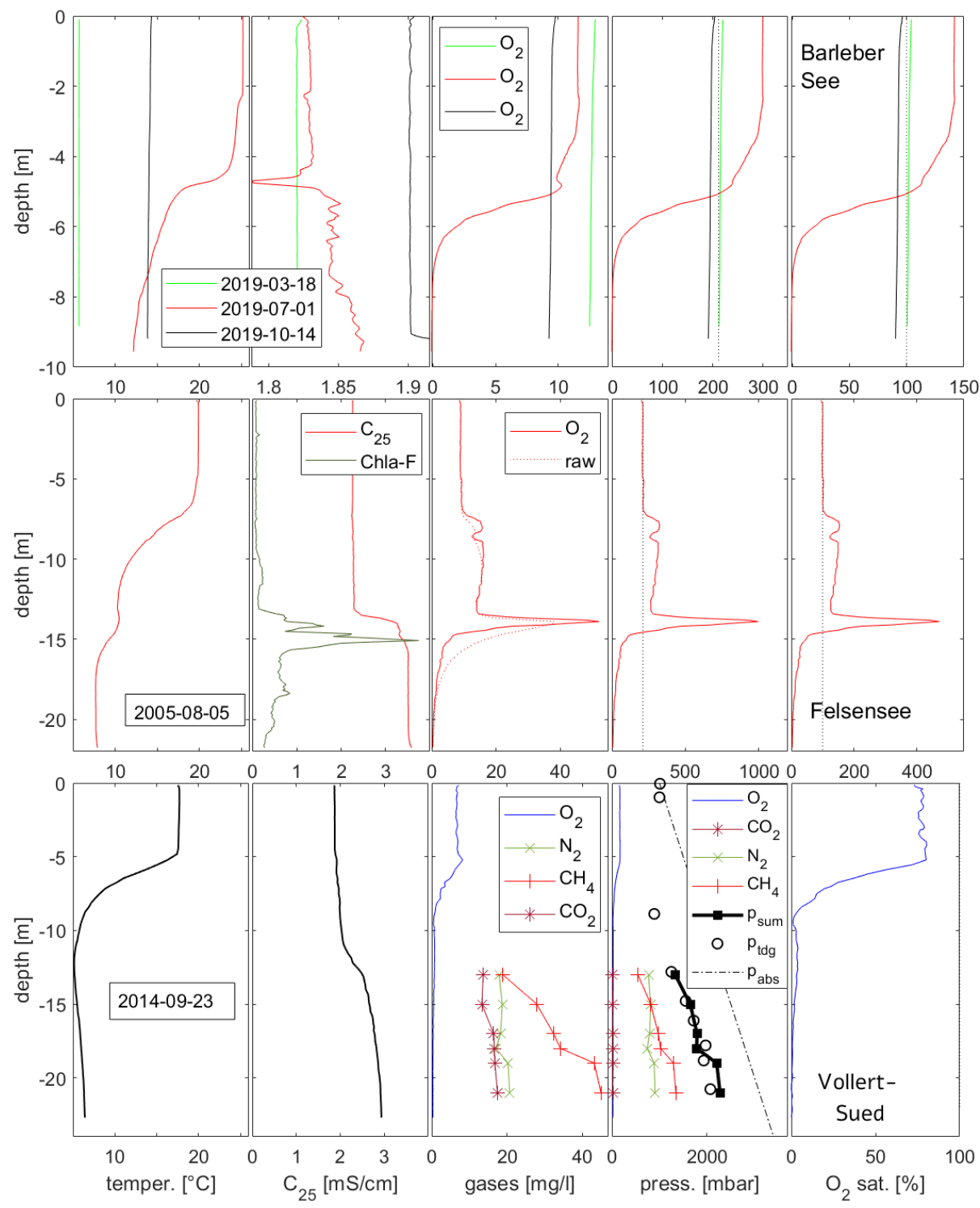
Table 1.
Henry coefficients (from [19] Sander, 2015); volumetric portion in dry atmosphere (N2, O2, Ar from [20] Roedel 1992, CO2 from [21] Worch 2015, CH4 by [22] Saunois et al. 2020); Ostwald coefficient calculated from values in [19] and coefficients for Equation (4) for N2 and O2 ([23] Weiss 1970), Ar ([24] Jenkins et al. 2019), CH4 ([25] Wiesenburg and Guinasso 1979) and CO2 ([26] Weiss 1974); changes due to the introduction of the new temperature standard ITS-90 in 1990 are too small to show up on our scale and temperature range.
| Atmosphere | kH (25 °C) | kH (25 °C) | TE | kH (25 °C) | A1 | A2 | A3 | u | |
|---|---|---|---|---|---|---|---|---|---|
| [%] | [mol/m3/Pa] | [mol/L/bar] | [K] | [-] | Coefficients for Equation (4) | ||||
| N2 | 78.09 | 6.4 × 10⁻⁶ | 6.4 × 10⁻⁴ | 1300 | 0.016 | −59.6274 | 85.7661 | 24.3696 | 986.9/ 22391 |
| O2 | 20.95 | 1.3 × 10⁻⁵ | 1.3 × 10⁻³ | 1500 | 0.032 | −58.3877 | 85.8079 | 23.8439 | |
| Ar | 0.93 | 1.4 × 10⁻⁵ | 1.4 × 10⁻³ | 1400 | 0.035 | −55.6578 | 82.0262 | 22.5929 | |
| CH4 | 0.00019 | 1.4 × 10⁻⁵ | 1.4 × 10⁻³ | 1600 | 0.035 | −68.8862 | 101.4956 | 28.7314 | |
| CO2 | ~0.039 | 3.3 × 10⁻⁴ | 3.3 × 10⁻² | 2400 | 0.82 | −58.0931 | 90.5069 | 22.2940 | 1/ 1.01325 |
Table 2.
Properties of the investigated lakes (residence time was calculated as volume by outflow); the origin of the data is supplied in the text of Section 3.1 for each lake in separate.
Table 2.
Properties of the investigated lakes (residence time was calculated as volume by outflow); the origin of the data is supplied in the text of Section 3.1 for each lake in separate.
| Lake Name | Surface Area [km2] | Volume [106 m3] | Max. Depth [m] | Inflow [106 m3/y] | Outflow [106 m3/y] | Residence Time [y] | Age in 2020 [y] | Origin |
|---|---|---|---|---|---|---|---|---|
| Arendsee | 5.1 | 149 | 49 | 6.03 | 2.65 | 56 | >10,000 | Dissolution of salt dome and subsidence |
| Rappbode Reservoir | 3.95 | 113 | 89 | 109.8 | 89.6 | 0.942 | 61 | Artificial dam |
| Rassnitzer See | 3.1 | 68 | 38 | 2.07 | 0.4 | 170 | 18 | Lignite surface mine |
| Barleber See | 1.03 | 6.9 | 9.8 | 1.18 | 0.53 | 13 | 88 | Gravel and sand excavations |
| Felsensee | 0.085 | Unknown (~1) | 22 | little GW flow | little GW flow | Unknown | >55 | Stone quarry |
| Vollert-Sued | 0.09 | 2 | 27 | 0.055 | 0.005 | 400 | 51 | Polluted opencast lignite mine |
Publisher’s Note: MDPI stays neutral with regard to jurisdictional claims in published maps and institutional affiliations. |
© 2021 by the authors. Licensee MDPI, Basel, Switzerland. This article is an open access article distributed under the terms and conditions of the Creative Commons Attribution (CC BY) license (https://creativecommons.org/licenses/by/4.0/).
Share and Cite
MDPI and ACS Style
Boehrer, B.; Jordan, S.; Leng, P.; Waldemer, C.; Schwenk, C.; Hupfer, M.; Schultze, M. Gas Pressure Dynamics in Small and Mid-Size Lakes. Water 2021, 13, 1824. https://doi.org/10.3390/w13131824
AMA Style
Boehrer B, Jordan S, Leng P, Waldemer C, Schwenk C, Hupfer M, Schultze M. Gas Pressure Dynamics in Small and Mid-Size Lakes. Water. 2021; 13(13):1824. https://doi.org/10.3390/w13131824
Chicago/Turabian StyleBoehrer, Bertram, Sylvia Jordan, Peifang Leng, Carolin Waldemer, Cornelis Schwenk, Michael Hupfer, and Martin Schultze. 2021. "Gas Pressure Dynamics in Small and Mid-Size Lakes" Water 13, no. 13: 1824. https://doi.org/10.3390/w13131824
Note that from the first issue of 2016, this journal uses article numbers instead of page numbers. See further details here.