
Seasonal and Decadal Variations of the Variance of the Synoptic and Mesoscale Sea Level Variability in the Baltic Sea

1
Shirshov Institute of Oceanology, Russian Academy of Sciences, 117997 Moscow, Russia
2
Fedorov Institute of Applied Geophysics, Roshydromet, 129128 Moscow, Russia
3
Department of Oceanology, Lomonosov Moscow State University, 119991 Moscow, Russia
*
Author to whom correspondence should be addressed.
Water 2021, 13(13), 1785; https://doi.org/10.3390/w13131785
Submission received: 28 April 2021
/
Revised: 14 June 2021
/
Accepted: 25 June 2021
/
Published: 28 June 2021
(This article belongs to the Section Oceans and Coastal Zones)
Abstract
:The present study examines the seasonal and decadal changes of the variance of the synoptic (periods from 2 days to 30 days) and mesoscale (periods from 2 h to 2 days) sea level oscillations in the Baltic Sea. Long-term hourly sea level records were used at 12 tide gauges located in different parts of the sea. We used spectral analysis to estimate the variance for different time scales. The spectral density of sea level oscillations in the Baltic Sea has maximum values in winter when the cyclonic activity in the atmosphere is more intensive. The maximum variances of synoptic and mesoscale sea level oscillations are observed in winter, except for the heads of the Gulf of Finland (Gorny Institute) and Gulf of Riga (Pärnu), where the absolute maximum of is reached in November. The variances and from November to February are 2–3 and 5 times higher than in the summer. The values of and are characterized by high correlation up to 0.7–0.75 with wind variations and atmospheric indices (NAO, AO, and SCAND) in winter and low correlation in summer. The zonal wind and in Gorny Institute are characterized by wide areas of high coherence at periods of 0.7–4 years. At Gedser, decreased by 19%, and at Ratan it increased by 17% over 90 years. The values of over 90 years increased by 32% at Klagshamn, 36% at Ratan, and up to 60% at Kungsholmsfort.
1. Introduction
The Baltic Sea is a semi-enclosed shelf basin connected to the open ocean through the narrow shallow Danish straits. As a result, in the inland water basin, the sea level variability totally differs from the open ocean. The tides make a dominating contribution to the sea level variance in the marginal seas (up to 85–90%), but they are negligibly small in the Baltic Sea. The amplitude of the main diurnal and semidiurnal constituents is 2–3 cm, and the maximum tidal range is 20–23 cm [1,2]. The tides contribute less than 2% to the total sea level variance in the Baltic Sea [3]. The main contribution to the sea level variance at periods from hours to months is made by the components of meteorological origin: storm surges and seiches. These sea level oscillations are internal. Kulikov et al. [4] showed that external sea level oscillations in the Kattegat Strait penetrating the Baltic Sea are very weak: the amplitude of oscillations with a period of 10 days decreases 10 times.
Medvedev [3] has studied in detail the Baltic Sea level spectrum formation in a wide frequency range. The intra-annual variations with periods from month to year compose the largest part (42–53%) of the total non-tidal sea level variance. The synoptic sea level variability contribution is 12% in the Baltic Proper, Stockholm, and 24% in the gulfs, Kronstadt and Furuogrund. Mesoscale non-tidal variability in the Baltic Sea is well pronounced in the Gulf of Finland and in the southwestern part of the sea. It amounts to 12%, while in the Gulf of Bothnia and Baltic Proper it does not exceed 2%.
Medvedev [5] has compared processed long-term observations at 48 coastal tide gauges and the ROMS numerical model results. It was found that the maxima in the spatial distribution of the synoptic sea level variance are located in the head of the Gulf of Bothnia and in the southwestern part of the Baltic Sea. The maximum variance of mesoscale sea level variance is located in the head of the Gulf of Finland and the southwestern regions of the sea.
Samuelsson and Stigebrandt [6] examined the interannual and seasonal variability of the sea level variance of the Swedish sea coast. They showed that the maximum variance at all stations corresponds to November and the minimum to the period from May to July. They divided the sea level variability into the five period ranges and showed that short-period oscillations from two days to two weeks prevail in the southern part of the Baltic, while long-period variations from two months to two years prevail in the Baltic Proper (Stockholm) and in the Gulf of Bothnia. Suursaar and Sooäär [7] showed that the annual standard deviations calculated based on hourly sea level at Pärnu rise statistically significantly by 2 cm in 1952–2004. Johansson et al. [8] found that standard deviations have increased by 1–3 cm for 50 years also at Finnish tide gauges. Both at Finnish and Estonian stations, the sea level variability was lower in the 1950s and higher in the 1980s [7].
Synoptic and mesoscale sea level variations in the Baltic Sea level are mainly influenced by meteorological factors, primarily the zonal wind [5]. From interannual to decadal timescales, the sea level oscillations are strongly determined by the strength of westerly winds [9]. This zonal component of wind variations is closely related to the North Atlantic Oscillation (NAO). For the Baltic Sea, the correlation between the NAO and mean sea level (MSL) is especially strong in winter [7,10,11,12], especially in the northern and eastern parts of the sea [13,14]. In the whole basin, the NAO–MSL correlation in winter changes significantly over time [9,15].
Medvedev [5] considered the temporal variability of the Baltic Sea level variance and found the link between winter NAO and the mesoscale sea level variance for the Gulf of Finland and for the Gulf of Riga. In the current research, we have extended this topic: seasonal and interdecadal changes in the variance of synoptic and mesoscale sea level oscillations in the Baltic Sea and the connection with atmospheric circulation were studied.
2. Materials and Methods
Long-term hourly sea level records at 12 coastal tide gauges located in different parts of the Baltic Sea were used to analyze synoptic and mesoscale sea level variability: Kalix, Furuogrund, Ratan, Stockholm, Kungsholmsfort, Klagshamn, Gedser, Warnemünde, Ristna, Pärnu, Narva, and the Gorny Institute (Figure 1). These stations are located in different parts of the Baltic Sea and have long-term quality sea level records. The length of the records varied from 31 to 127 years. Data were collected from the European Marine Observation and Data Network (EMODnet) (http://emodnet.eu/, accessed on 20 April 2021), the University of Hawaii Sea Level Center (UHSLC, http://uhslc.soest.hawaii.edu/, accessed on 20 April 2021), and the Unified State System of Information on the World Ocean (ESIMO, http://portal.esimo.ru/, accessed on 20 April 2021). All observations were brought to a single time reference (UTC). The series of observations were carefully checked, outliers and failures were removed, the short gaps were interpolated, and the series containing long gaps were excluded from the analysis.
Monthly data sets of wind at 10 m and atmospheric pressure at sea level were obtained from the 20th Century Reanalysis from 1871 to 2012 [16]. We used North Atlantic Oscillation (NAO) index data from Li and Wang [17]. The Arctic Oscillation (AO) index and the Scandinavia pattern (SCAND) index were taken from the NOAA Climate Prediction Center from 1950 to 2015.
Medvedev [3], based on the classification [18,19], identified five frequency bands of sea level variability: mesoscale, synoptic, intra-annual, seasonal, and interannual. In the current study, we are focused on the mesoscale and synoptic scales. The synoptic-scale has periods from 2 to 30 days, and the mesoscale has periods from 2 h to 2 days. The long-period storm surges contribute most of the synoptic-scale energy. Its generation is associated with atmospheric processes of the natural synoptic period. In turn, the mesoscale variability in the Baltic Sea is determined by the short-period storm surges and the natural sea level oscillations [20]. The main eigen mode period of the Baltic Sea and the Gulf of Finland is 26–29 h [20,21].
We used the fast Fourier transform (Welch’s method) for each year to calculate the sea-level spectra for each tide gauge. The linear trend was previously removed from the hourly series of observations. The variance of synoptic and mesoscale sea level variability was estimated as the sum of the spectral density values within the frequency band
where is the spectral resolution, and i varies for the synoptic-scale from 2 to 30 days, and for the mesoscale from 2 h to 2 days.
The wavelet coherence method was used to identify frequency bands in which time series of sea level and atmospheric processes are covarying [15,22]. The wavelet coherence of two signals x and y can be defined as
where is an operator that denotes smoothing along the wavelet scale axis and in time, and are wavelet-spectrums of signals x and y, and is the wavelet cross-spectrum [22]. This definition resembles the correlations coefficient, but only localized in frequency–time space.
3. Results
3.1. The Seasonal Variability of the Baltic Sea Level Spectra
We calculated spectra at nine tide gauges for four seasons (Figure 2): winter (DJF), spring (MAM), summer (JJA), and autumn (SON). The spectra were calculated for each separate 3-month time series and averaged over the full length of the records (31–127 years). There is a significant seasonal change in the spectral density of the continuum spectrum (continuum) in the synoptic frequency range~from 0.03 to 0.5 cpd for all stations. The highest values of spectral density are observed in winter. In spring, the spectral density in this frequency range decreases. It reaches its minimum in summer. Then it increases in autumn again. In spectra at most tide gauges, the maximum spectral density of the continuum is observed in winter, and it is less in autumn. However, in the head of the Gulf of Finland (Gorny Institute and Narva), the Gulf of Riga (Pärnu), and the Gulf of Bothnia (Kalix), the spectral density in winter and autumn does not differ. At the Gorny Institute, the autumn spectrum is even higher than in winter. This is probably due to the location of these tide gauges. The possible influence of the ice cover in the winter months can reduce the variance of the sea level oscillations of wind origin in the head of gulfs. The differences in the summer and spring spectra are negligible at the Gorny Institute, while at the other stations, the difference between the summer and spring spectra is significant.
The difference between the spectra at various seasons decreases with increasing frequency. Therefore, for the Gorny Institute, Pärnu, and Warnemünde, these spectra for four seasons merge. These tide gauges are located at the head of the bays, where the maximum amplitudes of seiches and the maximum of the variance of the mesoscale sea level oscillations in the Baltic Sea are observed [5]. At the other stations, in general, at the mesoscale, the same spectral pattern is observed as in the synoptic one. However, in the Gulf of Bothnia (Kalix and Furuogrund), the summer spectrum exceeds the spring one. This is possibly caused by the influence of the ice cover. In the spring, it still covers a significant area of the Gulf of Bothnia and thus prevents the formation of sea level oscillations with wind origin.
The spectral peaks with periods of 4, 5, 6, 7, and 8 cpd are observed at the summer spectrum of Narva. These peaks are less in the spectra of other seasons. This confirms the assumption of [1] that these peaks are radiational tides, and they are caused by the local influence of sea-breeze winds.
In general, the results of the spectral analysis showed a significant seasonal modification of the Baltic sea level spectrum. This seasonal variability is caused by seasonal changes of the driving forces, primarily, of the wind and atmospheric pressure fields and the cyclones trajectories.
3.2. Seasonal Changes of the Sea Level Variance
We calculated the variance of the synoptic and mesoscale sea level oscillations for individual months to obtain their seasonal variations. Figure 3 illustrates the results of these estimations for the synoptic scale. All tide gauges are characterized by a seasonal variation with a minimum in the summer and an increase of in November–December. The variances of from November to February are 2–3 times higher than in the summer. A small local maximum is observed at the Gorny Institute in May (Figure 3a). Probably, this variance maximum is formed under the influence of the Neva River runoff. In the head of the Gulf of Finland (Gorny Institute) and Gulf of Riga (Pärnu), the absolute maximum of is reached in November. At Narva and Ratan, it is reached in December, and at Stockholm and Kungsholmsfort in February. At the head of the Gulf of Finland, is 5–10 times greater than in the central part of the sea (Stockholm).
The seasonal variation of is generally similar to the seasonal variability: the minimum is in summer, and the maximum happens in December (Figure 4). However, if for all six stations increases by about 2–3 times more in the winter than in the summer, then is 5 times higher in the winter than in the summer. At the Gorny Institute (Figure 4a), a local maximum of is again found in May–June. A similar maximum is also observed at Pärnu, Narva, and Stockholm (Figure 4c–e).
The and values were calculated for every month of every year. We estimated the scatter of interannual variability in the estimates of and for each month; double standard deviation is shown in blue in Figure 3 and Figure 4. The weak standard deviations of are at Stockholm and Kungsholmsfort. The largest range of estimates fall on the head of the Gulf of Finland and the Gulf of Riga and probably are related to the instability of a larger number of factors causing sea level variability in this area. The standard deviations of in winter are 2–3 times stronger than in summer.
For each month we estimated trends in interannual changes in and estimates. For Swedish stations with long-term observation series (100 years or more), no significant trends in the interdecadal variability of and were revealed. Statistically significant trends by the Fisher test were identified for the Gulf of Finland and the Gulf of Riga. For these stations, we used relatively short sea level records (about 30 years). At these stations, there is a positive trend of in January and October and negative trends in September and December. At the Gorny Institute, positive trends were revealed for in January, while only negative trends were observed at Narva and Pärnu from September to October. It is likely that with an increase in the length of the analyzed series, the estimates of the trends in and may become less significant, which is observed in the example of Swedish stations with very long series of observations.
3.3. The Link between the Atmospheric Circulation, Wind, and Air Pressure in Different Seasons
Wind stress is one of the main factors determining sea level oscillations in the Baltic Sea [9]. In the current study, we analyzed the relationship between the and with changes in atmospheric pressure and wind over the Baltic Sea for each month. We used the monthly mean values of atmospheric pressure () and zonal () and meridional () wind components over the Baltic Sea from the 20th Century reanalysis. The length of the atmospheric time series corresponds to the full length of the tide gauge observations (e.g., 1978–2009 for Pärnu and Narva, 1889–2013 for Stockholm, see details in Table 1). The significance of the correlation coefficient was done using a t-test of the null hypothesis. The resultant 95% confidence level for nonzero correlation is 0.15–0.16 for Swedish tide gauges and 0.30–0.31 for short time series (Pärnu, Narva, Gorny Institute).
The pairs − and are characterized by negative correlation. The correlation coefficient in the synoptic-scale in all months at all stations varies from 0 to −0.54 without seasonality (Figure 5a). The correlation coefficient for the mesoscale decreases to −0.60 (Figure 5b). The eastern coast of the Baltic Sea (Gorny Institute, Narva, Pärnu) is characterized by a correlation coefficient of −0.6 in February, after which the correlation increases to almost zero in May and then decreases in June–July and September. On the western coast of the sea (Swedish stations), on the contrary, a correlation coefficient is about 0 in February and −0.4 in September.
The pairs and are characterized by a pronounced seasonal variation with maximum values of the correlation coefficient from November to March and minimum in May–July. For the synoptic scale, a sharp local maximum of the correlation coefficient is achieved in March: up to 0.70 at the Gorny Institute and up to 0.77 at Pärnu (Figure 5c). The correlation coefficient at Stockholm does not exceed 0.20 for the whole year. For the seasonal variation of the correlation coefficient has a similar character for all stations (Figure 5d). The eastern coast of the Baltic is characterized by a high correlation coefficient in January–March (up to 0.74 at the Gorny Institute and up to 0.80 at Pärnu) and a local maximum in November (up to 0.72) and May (up to 0.50–0.58). The seasonal correlation curve for Swedish stations is smoother. The minimum values were found at Ratan. This tide gauge is located in the Gulf of Bothnia, which has a meridional elongation, which, apparently, significantly reduces the effect of the zonal wind on the sea level oscillations in this gulf.
For the pairs , the correlation coefficient varies from −0.4 to 0.4 during the year, which indicates a lesser influence of the meridional wind on synoptic sea level variations (Figure 5e). For the Gulf of Finland and the Gulf of Riga, a correlation coefficient is from 0 to 0.4 from January to September, which indicates a small influence of the southerly wind on the formation of sea level variations on the synoptic scale. The correlation coefficient sharply changes its sign to negative in October–December and reaches −0.4 in November, which indicates the influence of the northerly wind on the sea level variations at the synoptic-scale in the autumn.
For the pairs , the correlation coefficient is higher than for (Figure 5f). In February, it is 0.55 for the eastern Baltic coast. The correlation coefficient sharply changes its sign to negative in April (up to −0.3), which again shows an increase in the role of northerly winds in the formation of sea level variations at the mesoscale. The absolute maximum of the correlation coefficient is reached in May, up to 0.65–0.67 in the Gulf of Finland, after which the coefficient decreases, and in November it already has negative values of up to −0.4 on the western Swedish seacoast.
Long-term changes in wind stress over the Baltic Sea are closely related to large-scale atmospheric circulation over the North Atlantic and numerically partially displayed in the North Atlantic Oscillation (NAO) index [17]. The NAO index is the pressure difference between the Azores maximum and the Icelandic minimum. The essence of the NAO lies in the redistribution of atmospheric masses between the Arctic and the subtropical Atlantic, while the transition from one phase of the NAO to another causes large changes in the wind field, heat, and humidity transfers, in the intensity, number, and trajectories of storms, etc. A positive NAO is characterized by the strong Azores High and Icelandic Low. It is associated with warm and humid winters and strong westerly winds in the Baltic Sea area, which cause sea level rise. A negative NAO (weak Azores High and Icelandic Low) is associated with cold and dry winters, which cause a sea-level decrease. The correlation between the Baltic Sea level and NAO is especially strong in winter [5,10].
In the current study, we examined the dependences of interannual changes in the and with changes in the NAO, the Arctic Oscillation (AO), and Scandinavian (SCAND) indices.
The AO is a large-scale mode of climate variability. It is also known as the Northern Hemisphere annular mode [23]. The AO pattern is characterized by winds circulating counterclockwise around the Arctic at around 55° N latitude. In the positive phase of this pattern, a belt of strong winds circulating the North Pole confines colder air across Polar Regions. When the AO is in a negative phase, this wind belt becomes weaker and more distorted. It allows colder, arctic air masses to penetrate southward more easily, and also the storminess increases into the mid-latitudes.
The Scandinavia pattern SCAND consists of a primary circulation center over Scandinavia, with weaker centers of an opposite sign over Western Europe and eastern Russia [24,25]. The positive phase of this pattern is associated with below-average temperatures over western Europe and across central Russia, sometimes reflecting major blocking anticyclones over Scandinavia and western Russia. It is also characterized by above-average precipitation across central and southern Europe and below-average precipitation across Scandinavia.
We estimated the correlation coefficients between and and the atmospheric circulation indices in different months. For the pairs of time series − NAO, − NAO, − AO, and − AO, a predominantly positive correlation coefficient is characteristic, while for the pairs − SCAND and − SCAND, the correlation coefficient was mostly negative. This is due to the different directions of the pressure gradient in the calculation of these atmospheric indices. The resultant 95% confidence level for nonzero correlation is 0.21–0.23 for Swedish tide gauges and 0.30–0.31 for short time series (Pärnu, Narva, Gorny Institute).
The largest values of the modulus of the correlation coefficient are observed in the period from November to March (Figure 6). The correlation approaches zero in the summer. The correlation coefficient at the head of the Gulf of Finland and the Gulf of Riga (Gorny Institute, Narva, and Pärnu) is higher than in the Gulf of Bothnia (Ratan) or in the Baltic Proper (Stockholm). The value of the correlation coefficient for the atmospheric circulation indices and for individual months is less than for .
At the Gorny Institute, Narva, and Kungsholmsfort, the correlation coefficient between the variance and the NAO index reaches the highest values in March, 0.40–0.45 (Figure 6a). The relationship between and the AO index at six tide gauges is slightly higher than with NAO. The correlation coefficient between changes in the AO index and at Pärnu is 0.57 in March (Figure 6c). The largest values of the modulus of the correlation coefficient are found with the SCAND index (Figure 6e). At the Gorny Institute, Narva, and Kungsholmsfort, the correlation coefficient with the SCAND index is −0.60–−0.65, and in November, high correlation coefficients between and the SCAND index are found not only in the Gulf of Finland (up to −0.64) and the Gulf of Riga (−0.50) but also at Ratan (−0.64) and Kungsholmsfort (−0.67). The correlation coefficients between and the NAO and AO indices in November are rather low at all stations, 0.08–0.15.
The seasonal variations of the correlation coefficient calculated for pairs of time series of and circulation indices have a similar form: maximum values in winter and about 0.10–0.20 in summer. At the Gorny Institute, Narva, and Pärnu stations, the correlation coefficient between and the NAO index has the highest values in February–March, 0.55–0.59 (Figure 6b). The relationship between and the AO index is even higher in February–March at these stations, up to 0.65–0.70 (Figure 6d). The SCAND index also shows a high correlation coefficient, but with the opposite sign, −0.69 (Figure 6f). The correlation coefficient with the SCAND index at Kungsholmsfort in January is −0.73. In November, a high correlation with all atmospheric indices is observed.
3.4. Interannual Changes in Sea Level Oscillations Variance
The variance of synoptic () and mesoscale () sea level oscillations changes from year to year. Medvedev [5] has shown that interannual changes in are in phase in different areas of the Baltic Sea (Ratan, Stockholm, and Kungsholmsfort) and do not have significant trends from XX to XXI centuries. In the interannual changes in , no significant trends were found either. Additionally, Medvedev [5] has shown that if we calculate the trends for observations from 1922 to 2010, then a pronounced positive trend was found at Ratan, Kungsholmsfort, and Stockholm: from 0.04 cm2/year at Ratan to 0.14 cm2/year at Kungsholmsfort. In the current study, we investigated the temporal changes of and in more detail.
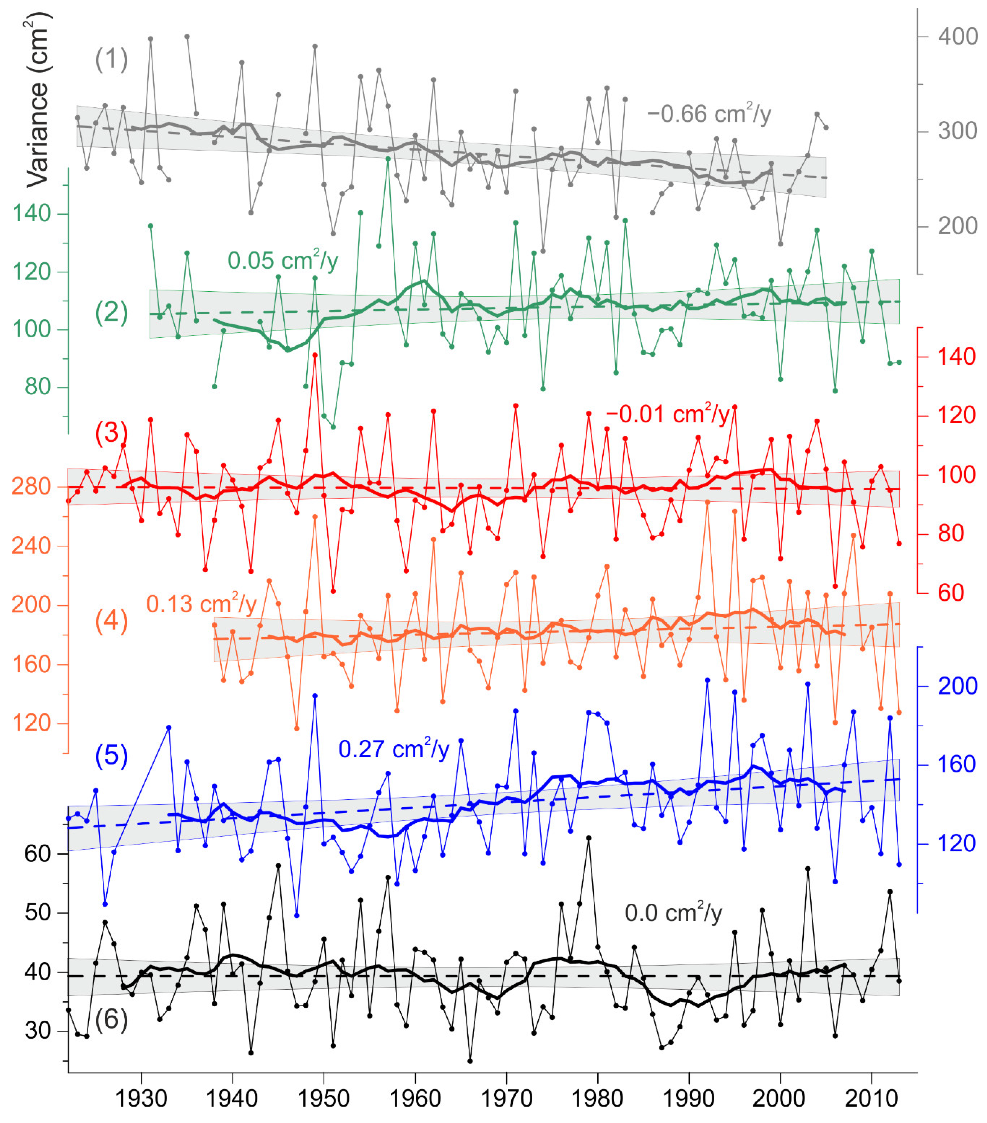
We estimated and for each year. Figure 7 shows interannual changes in at six tide gauges with long-term observation series from 1922 to 2013. The values change greatly from year to year. The standard deviation of interannual changes of value of are from 7 cm2 at Stockholm to 50 cm2 at Gedser, which is 16–19% of the long-term average values. A pronounced negative trend of −0.66 cm2/year was detected at Gedser, i.e., decreased by 19% over 90 years. At Ratan, an increase in with a rate of 0.27 cm2/year is observed, as a result of which the average value of over 90 years increased by 17%.
In general, interannual changes in at different tide gauges of the Baltic Sea are similar. The local annual highs and lows of are synchronously observed in different areas of the sea. For example, the local maximum in 1949 and the local minimum in 2006 are expressed both in the southwestern Baltic (Gedser, Klagshamn, Kungsholmsfort) and in the Gulf of Bothnia (Furuogrund and Ratan). For two nearby tide gauges, Ratan and Furuogrund, the correlation coefficient was 0.91. Interannual variations of at Kungsholmsfort are closely related (0.5–0.6) to the southwestern part of the Baltic (Gedser and Klagshamn), in the Gulf of Bothnia (Furuogrund), in the Baltic Proper (Stockholm), and in the Gulf of Riga (Pärnu). Some tide gauges have a relatively weak correlation with the other stations. At Ratan, the correlation coefficient with all the stations under consideration, except Furuogrund, does not exceed 0.40. The Gorny Institute has a correlation of less than 0.20 with most stations, except Gedser (0.40) and Pärnu (0.68). Pärnu has high correlation coefficients with the southwestern Baltic (Gedser, Klagshamn, and Kungsholmsfort) and with the Gorny Institute.
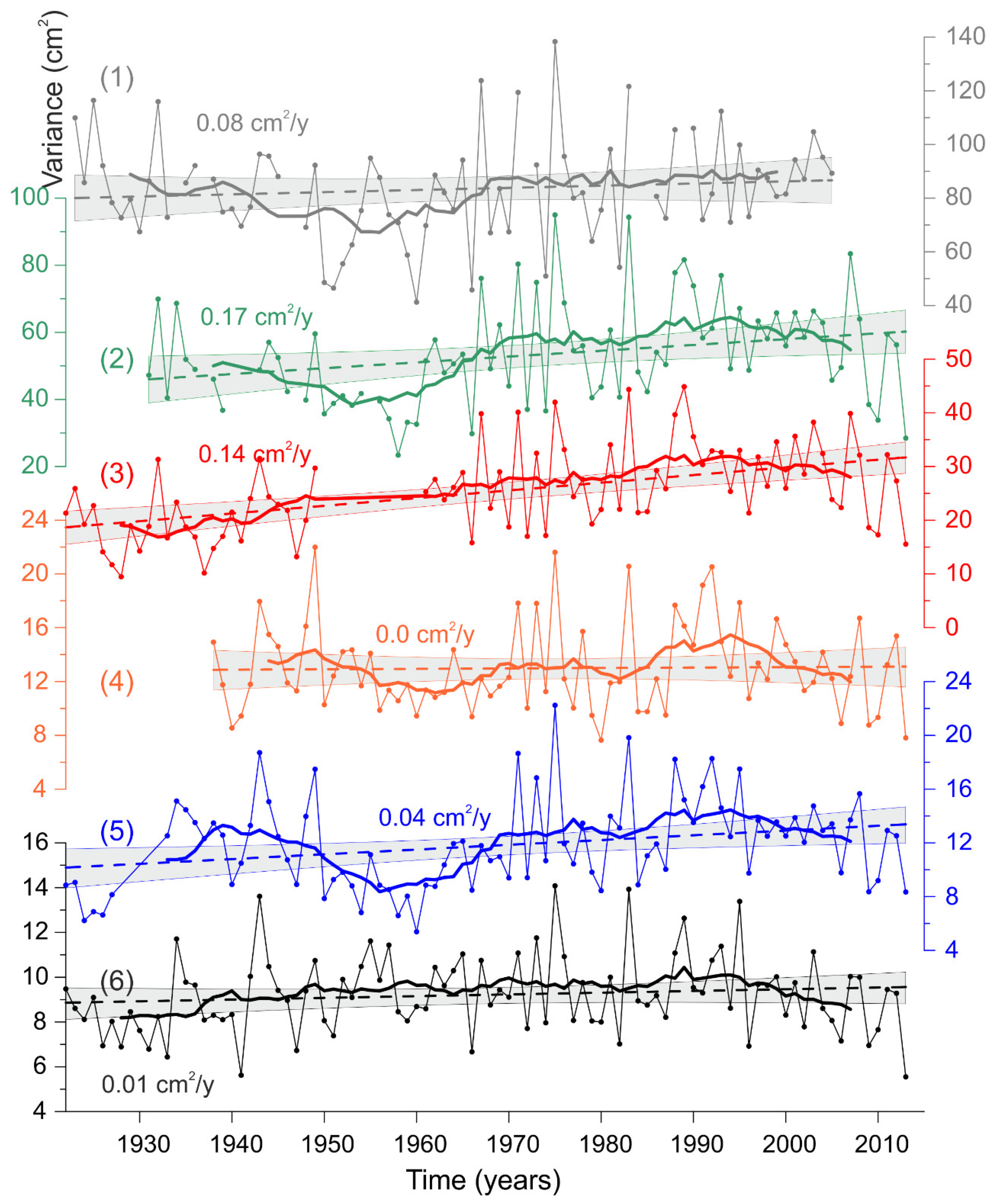
The variance of mesoscale sea level oscillations changes greatly from year to year (Figure 8). At Gedser, changes from 45 to 140 cm2, and at Ratan from 6 to 22 cm2. General periods of increase in , typical for most stations, were observed in 1936–1946, 1970–1979, and 1986–1995. Local minima of occurred in 1925–1933, 1953–1966, and 1980–1985. After 1996, a negative trend in is typical for most tide gauges. For the entire observation period (XX–XXI centuries), the absolute estimates of the rate of change of differ from 0 to 0.17 cm2/year, and these trends have significant values in relative units (for example, in percent). The trend at Gedser is 0.08 cm2/year, i.e., over 100 years, increased by 8 cm2, which is about 9–10% of the average value of for this station (85 cm2). For Klagshamn, 0.17 cm2/year is about 32% of the average (53 cm2), for Ratan up to 36% (average = 11 cm2), and for Kungsholmsfort up to 60% (average = 23 cm2).
We paid special attention to the change in the values of and from 1977–1978 and 2007–2013. Almost all stations have a negative trend in changes in and (Figure 9). The rate of changes from 0.22 cm2/year at the Gorny Institute to −0.71 cm2/year at Pärnu. At most stations, from 1977 to 2013 decreased by 4–7% from the average for this period. A significant trend was found at Pärnu, where the decreased from 184 in 1978 to 161 in 2009, i.e., by 23 cm2, which is 13% of the average value. A local minimum was observed at all stations from 1985 to 1991.
The rate of changes from 0.05 cm2/year at Kungsholmsfort to −1.02 cm2/year at Gorny Institute. At Ratan, Furuogrund, and Stockholm, the trend was −0.02–0.03 cm2/year, which ranges from 6% of the average at Ratan and up to 14% at Stockholm. The most intense decrease in in 1977–2009 was found at Pärnu, 19% of the average value of , and for the Gorny Institute, 26%. However, these trends of and have low statistical significance (see confidence limits in Figure 9). This is caused by the short period of time series and the large year-to-year variability of these values.
3.5. Relationship with Atmospheric Circulation, Wind, and Air Pressure Variations
In the current study, using cross-wavelet analysis, we estimated the coherence of changes in and with variations in the NAO and SCAND indices on a time-frequency scale. We used monthly data of atmospheric indices and values , for two tide gauges: Kungsholmsfort and the Gorny Institute. The coherence wavelet diagrams for in 1977–2006 have the same structure for NAO–Kungsholmsfort and NAO–Gorny Institute (Figure 10b,d): high coherence at the annual frequency and periods of 2–4 years. The Kungsholmsfort diagram shows high coherence for periods of 8–16 years in 1977–2006. The coherence between NAO and is very low for periods longer than 2 years from the 1890s to the 1960s. The NAO and coherence diagrams for two tide gauges have a similar structure to for 1977–2006. The long-term series of Kungsholmsfort is characterized by extremely high coherence over periods of more than 20 years for the entire 20th century.
The high coherence area moved from the annual cycle to a period of 1.5–3 years on the diagrams of the SCAND index and the values of and . This is found over the entire observation time (Figure 10e,f,h). Only for the pair SCAND— at the Gorny Institute is there no increase in coherence for periods longer than 1.5 years.
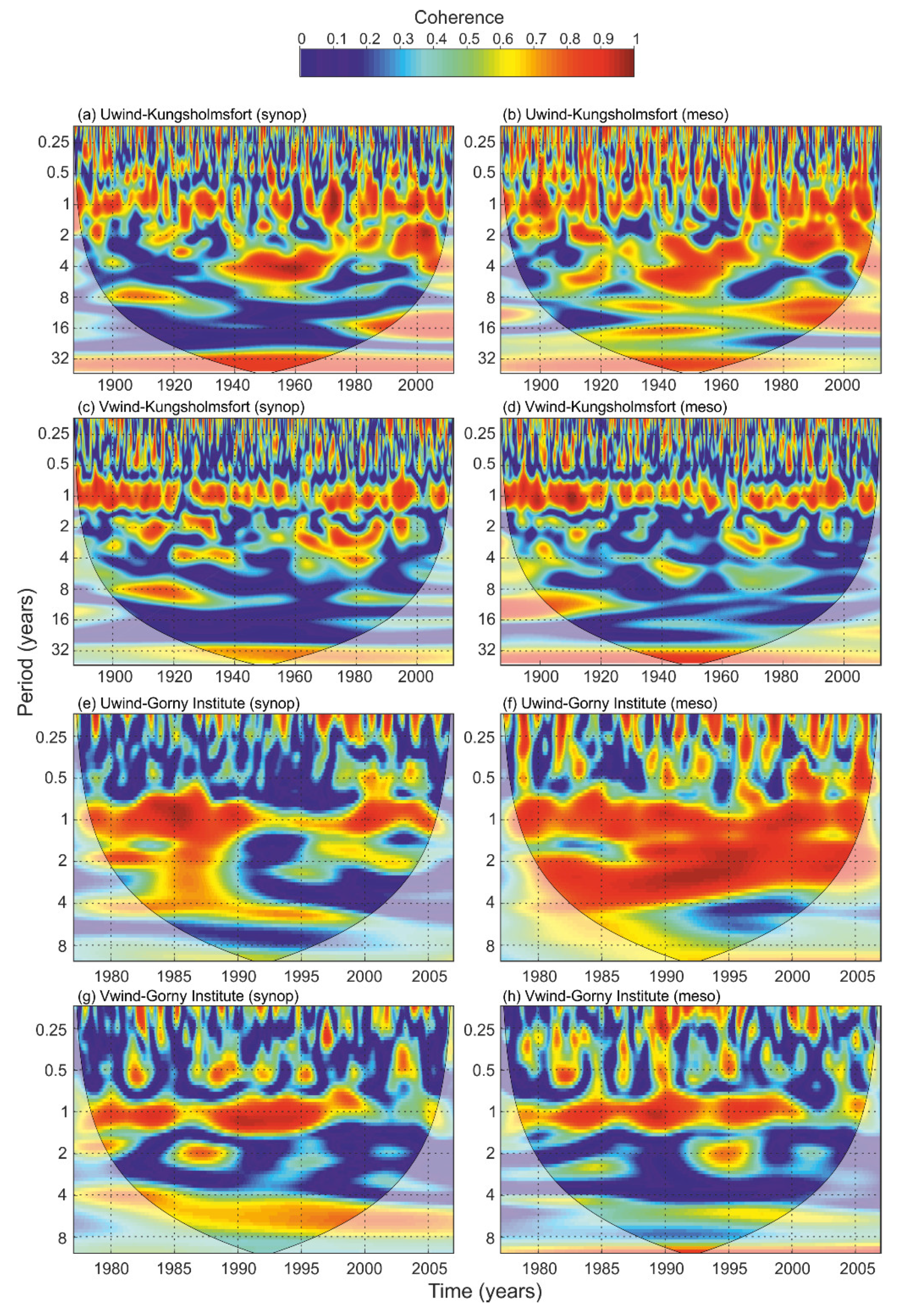
We estimated the wavelet coherence for pairs of monthly mean values of the zonal and meridional wind over the Baltic Sea and the values of and at Kungsholmsfort and the Gorny Institute. All diagrams of coherence are characterized by a regular increase of coherence at the annual frequency (Figure 11). The diagrams of the meridional wind have only local increases of coherence for periods longer than a year (Figure 11c,d,g,h). The zonal wind diagrams are characterized by wide areas of high coherence for longer than annual periods (Figure 11a,b,e,f). For the pair of at the Gorny Institute, an area of high coherence with periods from 0.7 to 4 years is observed throughout the observation period from 1977 to 2006 (Figure 11f).
4. Discussion
The main period of storm surges (floods) in the Gulf of Finland and the Gulf of Riga is about 24–30 h. Storm surges contribute a lot to the variance of mesoscale sea level oscillations in the Baltic Sea. Storm surges are separate extreme events, and it is difficult to obtain an integral estimate of their energy in individual years. The approach presented in the current study allowed us to obtain these estimates of the energy of storm surges, to study their seasonal and interannual variability, and also to discover their connection with atmospheric processes at various time-frequency scales. In [5], it was shown that the spatial distribution of the variance of mesoscale sea level oscillations is a reflection of the energy of storm surges and floods in the Baltic Sea. In the Gulf of Finland, the Gulf of Riga, and the southwestern part of the sea, the is significantly greater than in the central part of the Baltic and in the Gulf of Bothnia, where the height of the storm surges is significantly lower.
At Stockholm and Kungsholmsfort, the absolute maximum of is observed in February. At Stockholm, the February peak of significantly exceeds all values in other months. This feature of the seasonal variation in February is caused by the influence of water exchange between the Baltic and North seas. The tide gauges on the southwestern and central coasts of the Baltic Sea have a sharp decline in the sea level in February when the mean sea level decreases continuously over 10–20 days. These events occur quite often (5–6 times a decade). In some years, the average sea level at Stockholm during 10 days decreases by 60 cm, which is more than the average height of storm surge in this part of the sea. No pronounced maximum of in February was found at the tide gauges on the eastern coast of the Baltic Sea (Gorny Institute, Narva, and Pärnu). The variance of the storm surges in these eastern gulfs in the autumn–winter has higher magnitudes than a sharp decline in the sea level in February. Lehmann and Post [26] introduced a new term “Large Volume Changes (LVCs)”, which represents sea level increases by at least 29 cm, which corresponds to 100 km3 of the Baltic Sea volume change. They detected 74 LVCs in filtering Landsort sea surface elevation anomalies daily time series for 1948–2013. LVC leads to high values of in February at Stockholm and Kungsholmsfort.
In general, the same consistent pattern is observed in the seasonal variations of and on the entire coast of the Baltic Sea: low values in summer and high values in autumn–winter. The same seasonal features are characteristic of storm surges in the Baltic Sea, which is associated with the intensification of cyclonic activity in the atmosphere in autumn–winter. The total sea level variance in the Baltic Sea has the same seasonal changes. Samuelsson and Stigebrandt [6] showed that the maximum of mean monthly variance at Swedish tide gauges is observed in November and the minimum in May and July. They showed that externally forced sea level (caused by the varying sea level outside in the North Sea) explains most of the variance for periods longer than one month in the central parts of the sea (Stockholm). These external sea level variations are associated with the LVCs and can influence the variations with periods longer than 10 days.
The atmospheric circulation is the main factor determining the seasonal and interannual changes of and . Moreover, the zonal wind is the main factor affecting the variance of the sea level oscillations at these frequencies. If the correlation with atmospheric indices in winter reaches 0.6–0.7, then the correlation coefficient with zonal wind increases to 0.8 in winter. As it is known, the Baltic Sea level variations on a wide frequency range are determined mainly by atmospheric processes, and one of the main factors is the wind effect. This factor determines long-term sea level changes in the Baltic Sea [10,15,27,28,29,30,31,32,33] and short-term sea level oscillations in the synoptic and mesoscale ranges [4,20].
The seasonal changes of the correlation coefficient in Section 3.3 and Section 3.4 were shown for the different length time series. We additionally counted the same correlation coefficients using the time span (1978–2006) for all stations. The main properties described in Section 3.3 and Section 3.4 do not change.
Bednorz and Tomczyk [34] found the relationships between atmospheric conditions and changes in the Baltic Sea level on high- and low-frequency scales. In the cold season the rapid increases in the Baltic Sea level exceeding 24 cm within a 5-day period are associated with the development of specific synoptic conditions in the Euro-Atlantic region. It is characterized by a shift from high to low pressure over Europe and a rapid increase in the pressure gradient during the week preceding the sea level rise. Among macroscale circulation patterns, the SCAND is most relevant to the low-frequency variability of the Baltic Sea level [34]. For the synoptic frequency range, our results are in good agreement with their conclusions.
Suursaar and Sooäär [7] noticed that the annual standard deviations at Parnu show a rise from 26.5 to 28.5 cm for the period 1952–2004. Johansson et al. [8] showed that also at Finnish tide gauges standard deviations have increased by 1–3 cm over a period of 50 years. In the 1980s, the annual standard deviations at Estonian and Finnish tide gauges reached a maximum and decreased afterward. We also found the positive tendencies in the interannual changes for long records (80–90 years) and negative tendencies for short time series (Figure 9).
One of the most pressing challenges of science today is global climate change. Much attention is paid to climatic changes in the mean sea level of the World Ocean and changes in the return period and height of storm surges on the seacoast. In [8,9], the climatic variability of extreme sea level oscillations in the Baltic Sea was studied. Johansson et al. [8] identified significant trends in the increased frequency of extreme sea level rises on the Finnish coast of the Baltic Sea (Gulf of Finland and Gulf of Bothnia). Johansson et al. [8] used tide gauge data mainly from 1922. We found positive tendencies in the interannual changes of in 1922–2013 at a rate of up to 0.17 cm2/year (Figure 8).
5. Conclusions
The results of our study are in good agreement with the results of the earlier research of the other authors [6,7,8]. However, only Suursaar and Sooäär [7] and Johansson et al. [8] analyzed the interannual variations of the annual standard deviations of total sea level. Samuelsson and Stigebrandt [6] partitioned the total sea level variations at the different period bands, but their study only features the contributions of these bands to the total sea level variance for different stations. The present study examines seasonal and interannual changes of the variance of synoptic and mesoscale sea level oscillations in the Baltic Sea and their links with atmospheric circulation. The study has some new interesting findings:
- The spectral density of the sea level oscillations in the Baltic Sea has maximum values in winter when the cyclonic activity in the atmosphere is more intensive. However, in the head of the Gulf of Finland (Gorny Institute), the autumn spectrum is even higher than winter, which can be explained by the influence of the ice cover, which can reduce the sea level oscillations of wind origin.
- The maximum variance of synoptic and mesoscale sea level oscillations is observed in winter, except the heads of the Gulf of Finland (Gorny Institute) and Gulf of Riga (Pärnu), where the absolute maximum of is reached in November. The variances and from November to February are 2–3 and 5 times higher than in the summer.
- The values of and are characterized by high correlation (up to 0.70–0.75) with wind variations and atmospheric indices in winter and low correlation in summer.
- The diagrams of wavelet coherence of the meridional/zonal wind, atmospheric indices, and and are characterized by high values at the annual frequency. The zonal wind and at the Gorny Institute are characterized by wide areas of high coherence for periods of 0.7–4 years.
- The and values change greatly from year to year. At Gedser, decreased by 19%, and at Ratan it increased by 17% over 90 years. The values of for 90 years increased by 32% at Klagshamn, 36% at Ratan, and up to 60% at Kungsholmsfort.
The obtained results contribute to the knowledge of the sea level oscillations in the Baltic Sea and its climate changes.
Author Contributions
I.M. jointly developed the concept of the study. I.M. performed the analysis, visualization, and manuscript writing. A.M. performed the analysis and visualization. All authors have read and agreed to the published version of the manuscript.
Funding
This research was partially supported by the Russian Science Foundation (Grant 20-77-00099) and the Russian State Assignment of IO RAS #0128-2021-0004.
Institutional Review Board Statement
Not applicable.
Informed Consent Statement
Not applicable.
Data Availability Statement
The data presented in this study are available on the websites of the European Marine Observation and Data Network (http://emodnet.eu/, accessed on 20 April 2021), the University of Hawaii Sea Level Center (http://uhslc.soest.hawaii.edu/, accessed on 20 April 2021), and the Unified State System of Information on the World Ocean (http://portal.esimo.ru/, accessed on 20 April).
Conflicts of Interest
The authors declare no conflict of interest.
References
- Medvedev, I.P.; Rabinovich, A.B.; Kulikov, E.A. Tidal oscillations in the Baltic Sea. Oceanology 2013, 53, 526–538. [Google Scholar] [CrossRef]
- Medvedev, I.P.; Rabinovich, A.B.; Kulikov, E.A. Tides in three enclosed basins: The Baltic, Black, and Caspian seas. Front. Mar. Sci. 2016, 3, 46. [Google Scholar] [CrossRef] [Green Version]
- Medvedev, I.P. Formation of the Baltic Sea level spectrum. Dokl. Earth Sci. 2015, 463, 760–764. [Google Scholar] [CrossRef]
- Kulikov, E.A.; Medvedev, I.P.; Koltermann, K.P. Baltic sea level low-frequency variability. Dyn. Meteorol. Oceanogr. 2015, 67, 25642. [Google Scholar] [CrossRef]
- Medvedev, I.P. Spatial and temporal features of synoptic and mesoscale variability of the Baltic Sea level. Russ. Meteorol. Hydrol. 2018, 43, 815–826. [Google Scholar] [CrossRef]
- Samuelsson, M.; Stigebrandt, A. Main characteristics of the long-term sea level variability in the Baltic Sea. Dyn. Meteorol. Oceanogr. 1996, 48, 672–683. [Google Scholar] [CrossRef] [Green Version]
- Suursaar, Ü.; Sooäär, J. Decadal variations in mean and extreme sea level values along the Estonian coast of the Baltic Sea. Dyn. Meteorol. Oceanogr. 2007, 59, 249–260. [Google Scholar] [CrossRef]
- Johansson, M.; Boman, H.; Kahma, K.K.; Launiainen, J. Trends in sea level variability in the Baltic Sea. Boreal Environ. Res. 2001, 6, 159–180. [Google Scholar]
- Hünicke, B.; Zorita, E.; Soomere, T.; Madsen, K.S.; Johansson, M.; Suursaar, Ü. Recent change—Sea level and wind waves. In Second Assessment of Climate Change for the Baltic Sea Basin, Regional Climate Studies; The BACC II Author Team, Ed.; Springer International Publishing: Cham, Switzerland, 2015; pp. 155–185. [Google Scholar]
- Andersson, H.C. Influence of long-term regional and large-scale atmospheric circulation on the Baltic sea level. Dyn. Meteorol. Oceanogr. 2002, 54A, 76–88. [Google Scholar] [CrossRef]
- Dailidienė, I.; Davulienė, L.; Tilickis, B.; Stankevičius, A.; Myrberg, K. Sea level variability at the Lithuanian coast of the Baltic Sea. Boreal Environ. Res. 2006, 11, 109–121. [Google Scholar]
- Hünicke, B.; Zorita, E. Influence of temperature and precipitation on decadal Baltic Sea level variations in the 20th century. Dyn. Meteorol. Oceanogr. 2006, 58, 141–153. [Google Scholar] [CrossRef] [Green Version]
- Johansson, M.M.; Kahma, K.K.; Boman, H.; Launiainen, J. Scenarios for sea level on the Finnish coast. Boreal Environ. Res. 2004, 9, 153–166. [Google Scholar]
- Suursaar, U.; Jaagus, J.; Kullas, T. Past and future changes in sea level near the Estonian coast in relation to changes in wind climate. Boreal Environ. Res. 2006, 11, 123. [Google Scholar]
- Jevrejeva, S.; Moore, J.C.; Woodworth, P.L.; Grinsted, A. Influence of large-scale atmospheric circulation on European sea level: Results based on the wavelet transform method. Dyn. Meteorol. Oceanogr. 2005, 57A, 183–193. [Google Scholar] [CrossRef]
- Compo, G.P.; Whitaker, J.S.; Sardeshmukh, P.D.; Matsui, N.; Allan, R.J.; Yin, X.; Gleason, B.E.; Vose, R.S.; Rutledge, G.; Bessemoulin, P.; et al. The twentieth century reanalysis project. Q. J. R. Meteorol. Soc. 2011, 137, 1–28. [Google Scholar] [CrossRef]
- Li, J.; Wang, J.X.L. A new North Atlantic Oscillation index and its variability. Adv. Atmos. Sci. 2003, 20, 661–676. [Google Scholar] [CrossRef]
- Monin, A.S.; Kamenkovich, V.M.; Kort, V.G. Variability of the Oceans; Wiley: Hoboken, NJ, USA, 1977. [Google Scholar]
- Kamenkovich, V.M.; Koshlyakov, M.N.; Monin, A.S. Synoptic Eddies in the Ocean; Springer Science & Business Media: Berlin, Germany, 1986; Volume 5. [Google Scholar]
- Kulikov, E.A.; Medvedev, I.P. Variability of the Baltic Sea level and floods in the Gulf of Finland. Oceanology 2013, 53, 145–151. [Google Scholar] [CrossRef]
- Wubber, C.; Krauss, W. The two-dimensional seiches of the Baltic Sea. Oceanol. Acta 1979, 2, 435–446. [Google Scholar]
- Grinsted, A.; Moore, J.C.; Jevrejeva, S. Application of the cross wavelet transform and wavelet coherence to geophysical time series. Nonlinear Process. Geophys. 2004, 11, 561–566. [Google Scholar] [CrossRef]
- Thompson, D.W.; Wallace, J.M. The Arctic Oscillation signature in the wintertime geopotential height and temperature fields. Geophys. Res. Lett. 1998, 25, 1297–1300. [Google Scholar] [CrossRef] [Green Version]
- Barnston, A.G.; Livezey, R.E. Classification, seasonality and persistence of low-frequency atmospheric circulation patterns. Mon. Weather Rev. 1987, 115, 1083–1126. [Google Scholar] [CrossRef]
- Bueh, C.; Nakamura, H. Scandinavian pattern and its climatic impact. Q. J. R. Meteorol. Soc. 2007, 133, 2117–2131. [Google Scholar] [CrossRef]
- Lehmann, A.; Post, P. Variability of atmospheric circulation patterns associated with large volume changes of the Baltic Sea. Adv. Sci. Res. 2015, 12, 219–225. [Google Scholar] [CrossRef] [Green Version]
- Heyen, H.; Zorita, E.; von Storch, H. Statistical downscaling of monthly mean North Atlantic air-pressure to sea level anomalies in the Baltic Sea. Dyn. Meteorol. Oceanogr. 1996, 48A, 312–323. [Google Scholar] [CrossRef] [Green Version]
- Bastos, A.; Trigo, R.; Barbosa, S.M. Discrete wavelet analysis of the influence of the North Atlantic Oscillation on Baltic Sea level. Dyn. Meteorol. Oceanogr. 2013, 65A, 20077. [Google Scholar] [CrossRef] [Green Version]
- Hünicke, B.; Zorita, E. Trends in the amplitude of Baltic Sea level annual cycle. Dyn. Meteorol. Oceanogr. 2008, 60A, 154–164. [Google Scholar] [CrossRef] [Green Version]
- Johansson, M.M.; Pellikka, H.; Kahma, K.K.; Ruosteenoja, K. Global sea level rise scenarios adapted to the Finnish coast. J. Mar. Syst. 2014, 129, 35–46. [Google Scholar] [CrossRef]
- Karabil, S.; Zorita, E.; Baehr, J. Mechanisms of variability in decadal sea-level trends in the Baltic Sea over the 20th century. Earth Syst. Dyn. 2017, 8, 1031–1046. [Google Scholar] [CrossRef] [Green Version]
- Medvedev, I.P.; Rabinovich, A.B.; Kulikov, E.A. The pole tide/14-month oscillations in the Baltic Sea during the 19th and 20th centuries: Spatial and temporal variations. Cont. Shelf Res. 2017, 137, 117–130. [Google Scholar] [CrossRef]
- Medvedev, I.; Kulikov, E. Low-frequency Baltic sea level spectrum. Front. Earth Sci. 2019, 7, 284. [Google Scholar] [CrossRef]
- Bednorz, E.; Tomczyk, A.M. Influence of macroscale and regional circulation patterns on low-and high-frequency sea level variability in the Baltic Sea. Theor. Appl. Climatol. 2021, 144, 115–125. [Google Scholar] [CrossRef]
Figure 1.
Locations of the tide gauges (circles) and reanalysis grid point (square) with the wind and pressure data.
Figure 1.
Locations of the tide gauges (circles) and reanalysis grid point (square) with the wind and pressure data.
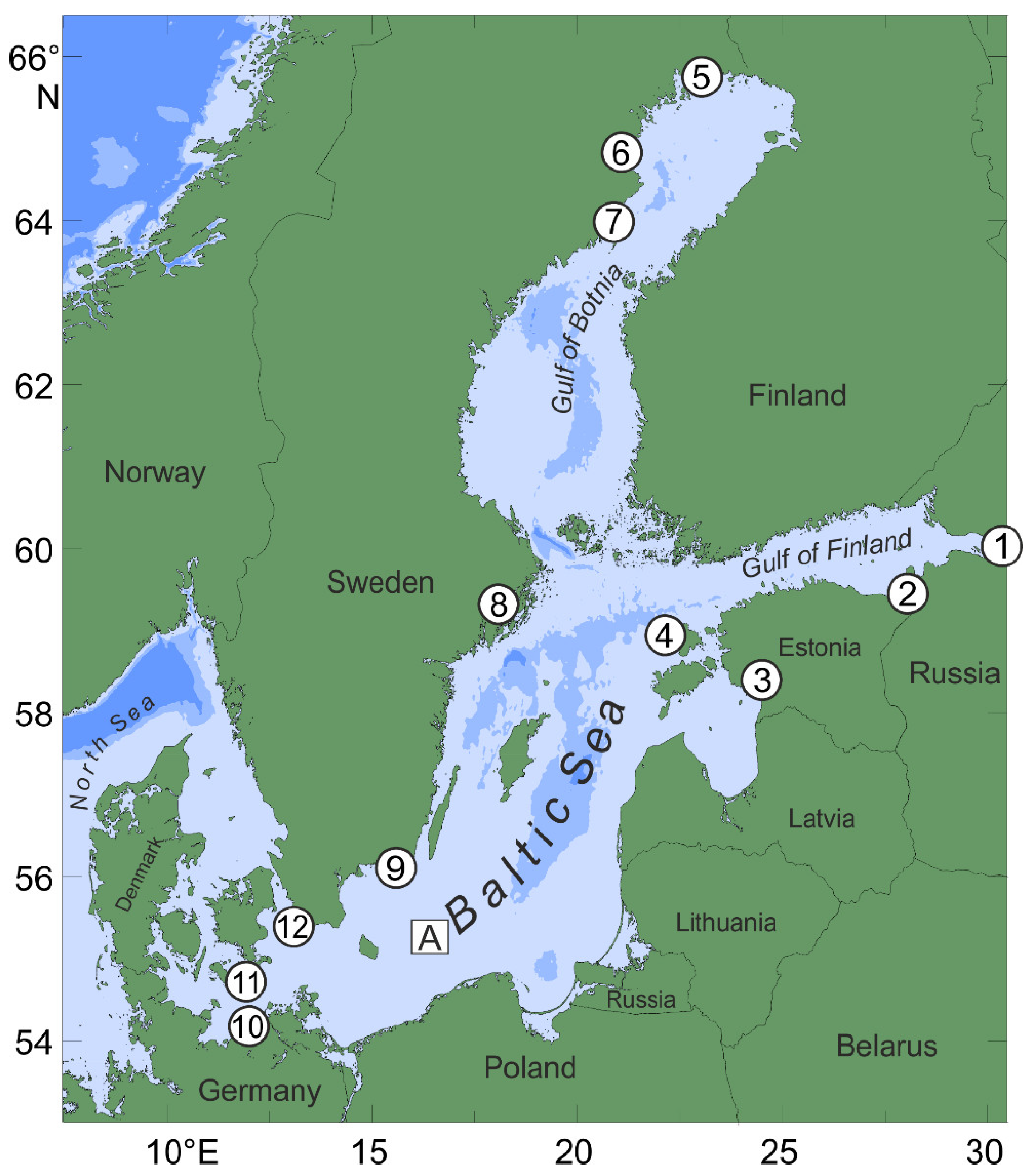
Figure 2.
Seasonal spectra of the sea level oscillations at nine Baltic Sea stations: (a) Gorny Institute, (b) Narva, (c) Pärnu, (d) Ristna, (e) Furuogrund, (f) Kalix, (g) Stockholm, (h) Kungsholmsfort, (i) Warnemünde.
Figure 2.
Seasonal spectra of the sea level oscillations at nine Baltic Sea stations: (a) Gorny Institute, (b) Narva, (c) Pärnu, (d) Ristna, (e) Furuogrund, (f) Kalix, (g) Stockholm, (h) Kungsholmsfort, (i) Warnemünde.
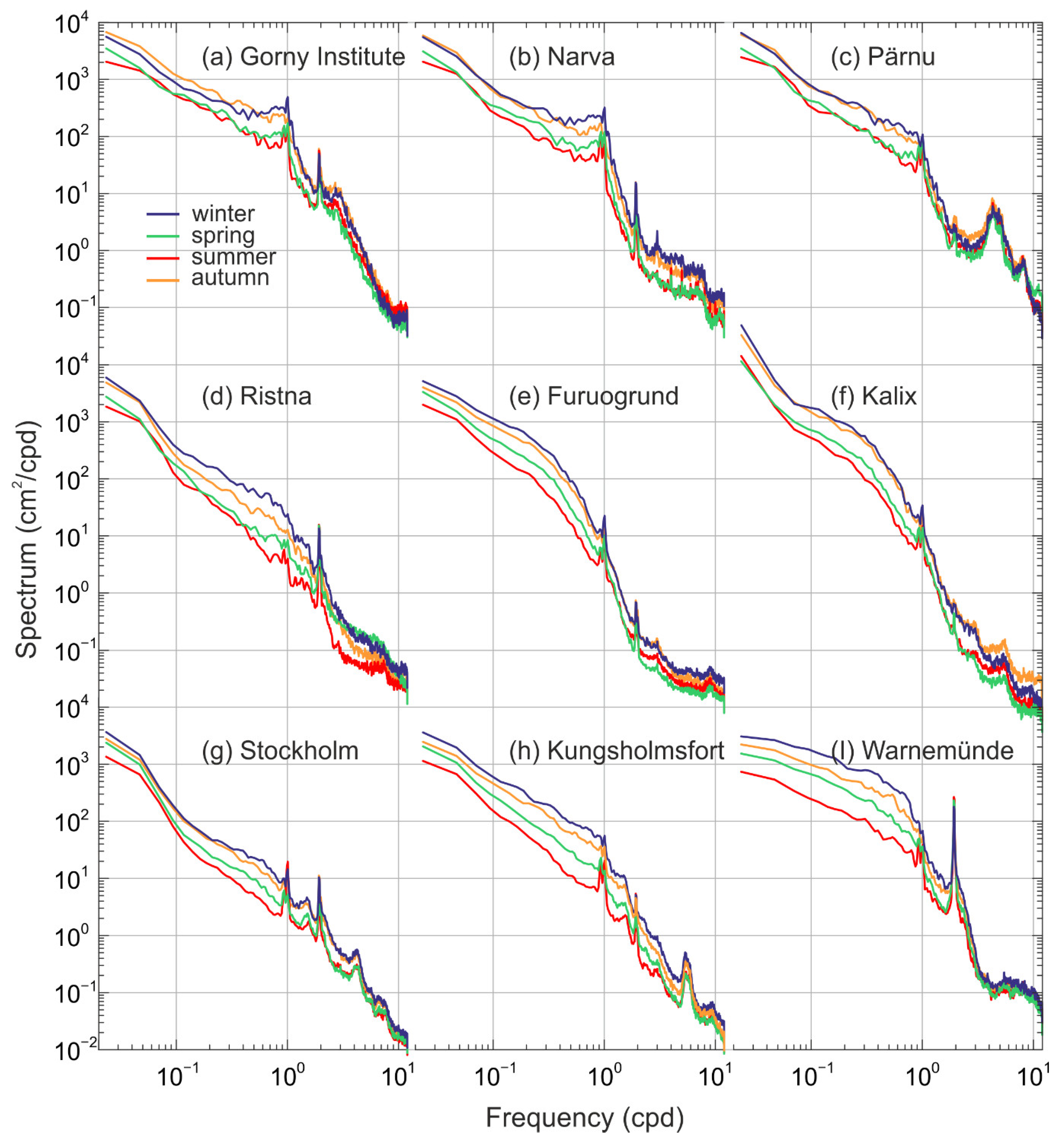
Figure 3.
Seasonal changes of the variance of synoptic oscillations () for stations at (a) the Gorny Institute, (b) Ratan, (c) Narva, (d) Stockholm, (e) Pärnu, and (f) Kungsholmsfort. The light blue color is ± standard deviations of interannual changes of , blue vectors are trends of its value: up is positive, down is negative, right is no trend.
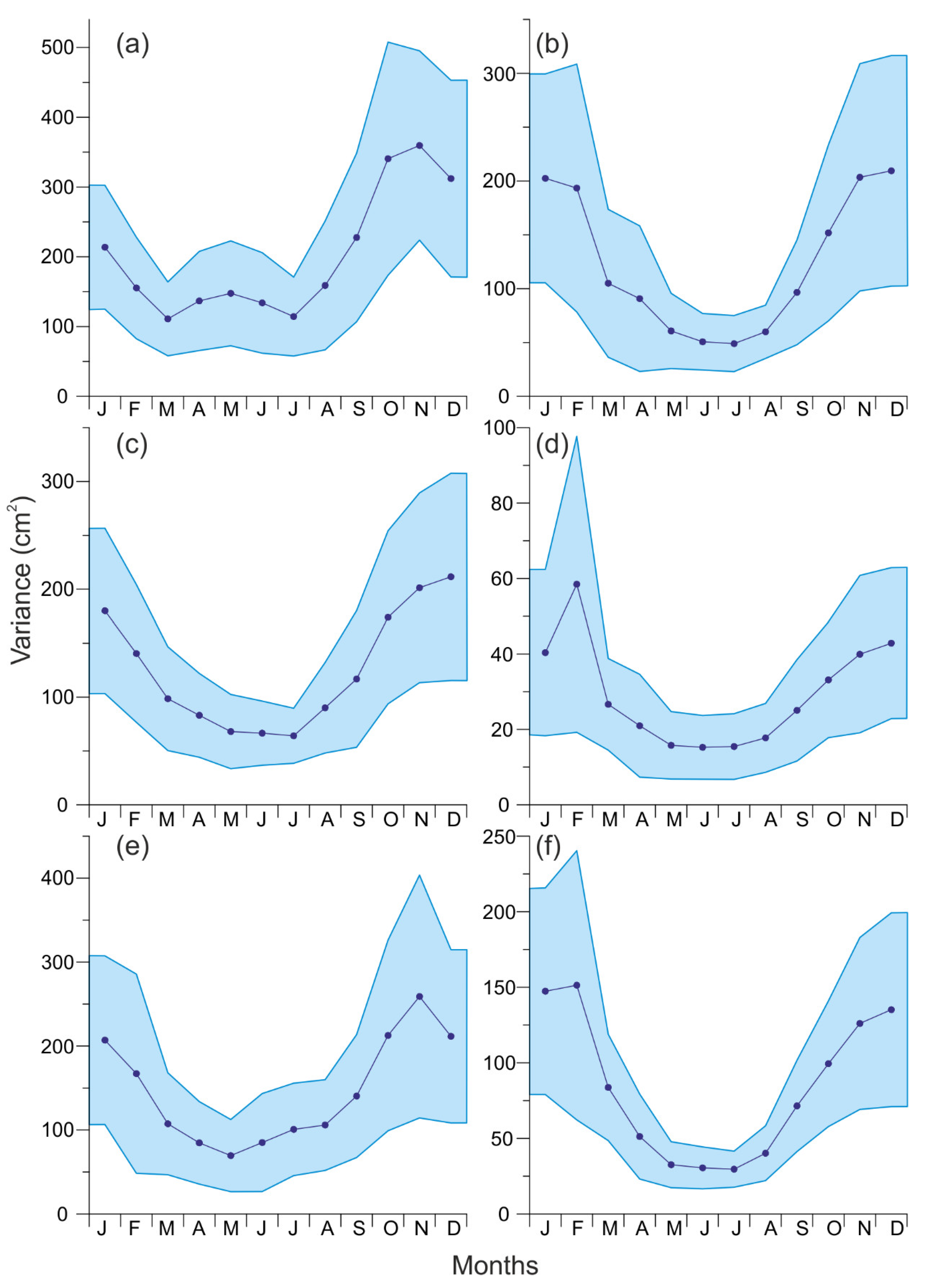
Figure 4.
Seasonal changes of the variance of the mesoscale sea level oscillations () for stations at (a) the Gorny Institute, (b) Ratan, (c) Narva, (d) Stockholm, (e) Pärnu, and (f) Kungsholmsfort. The light blue color is ± standard deviations of interannual changes of , blue vectors are trends of its value: up is positive, down is negative, right is no trend.
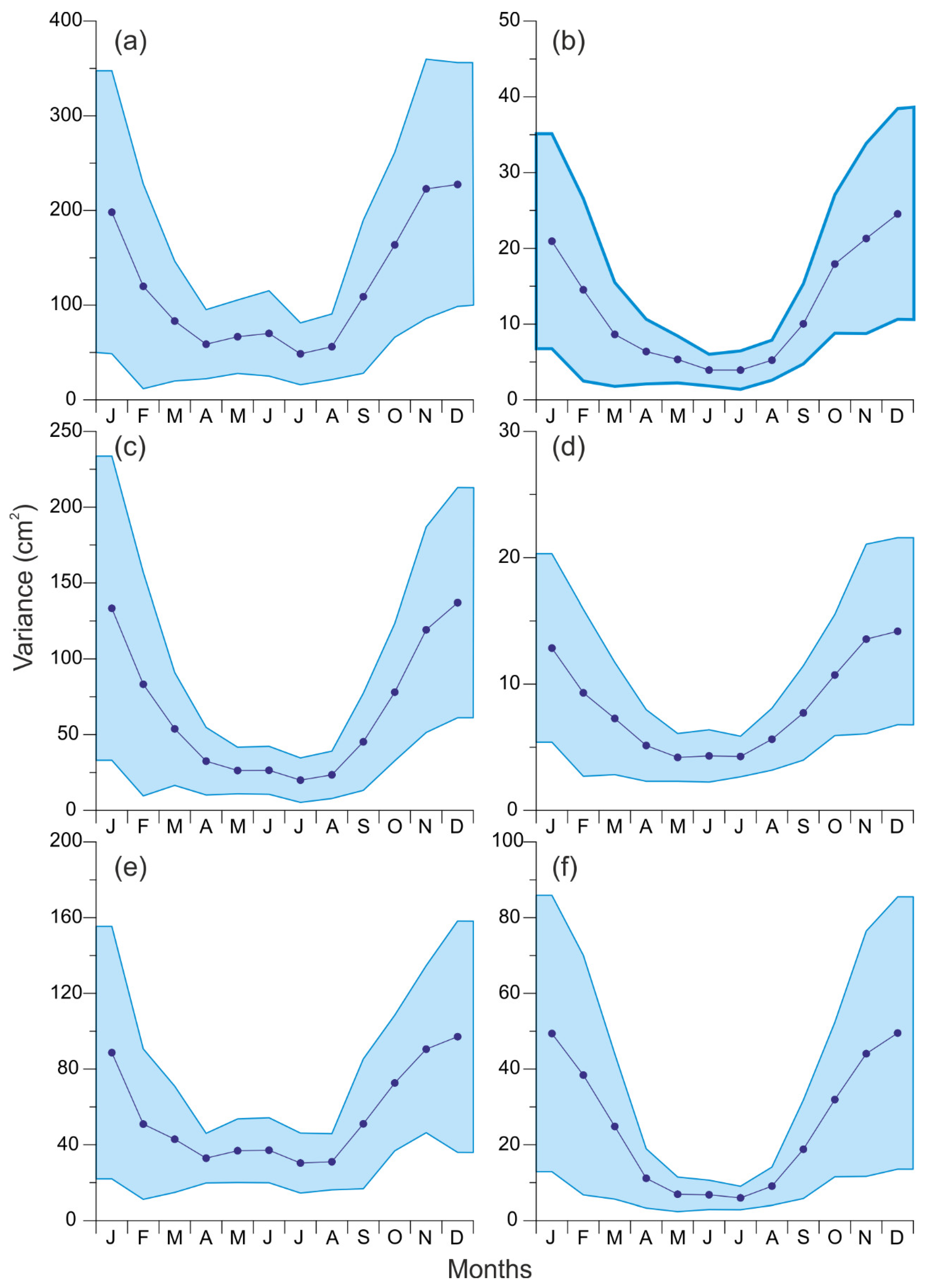
Figure 5.
Correlation coefficient (R) of the variance of (a,c,e) synoptic and (b,d,f) mesoscale sea level oscillations and monthly mean values of (a,b) surface atmospheric pressure, (c,d) zonal, and (e,f) meridional winds in different months.
Figure 5.
Correlation coefficient (R) of the variance of (a,c,e) synoptic and (b,d,f) mesoscale sea level oscillations and monthly mean values of (a,b) surface atmospheric pressure, (c,d) zonal, and (e,f) meridional winds in different months.
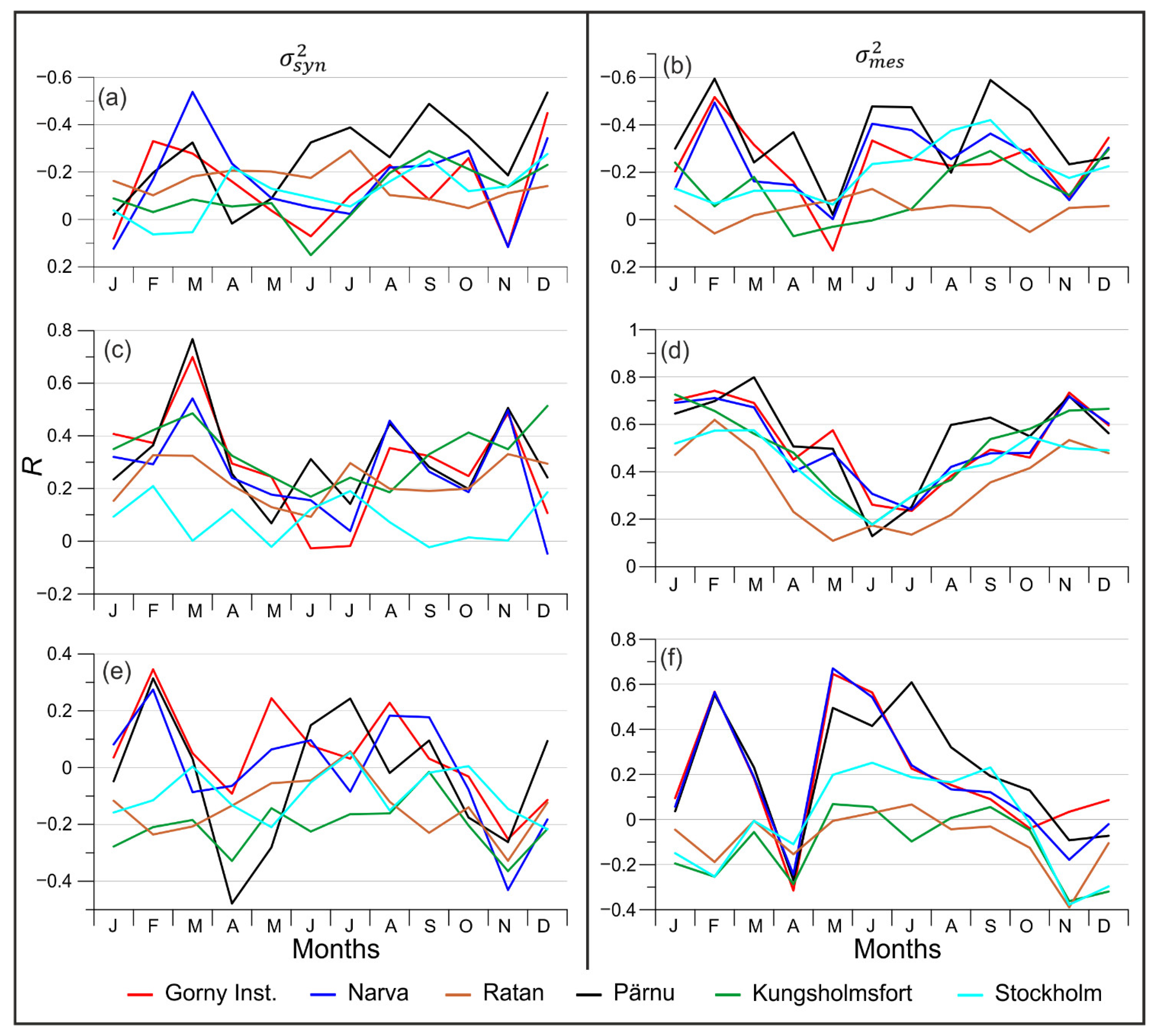
Figure 6.
Correlation coefficient (R) of the variance of (a,c,e) synoptic and (b,d,f) mesoscale sea level oscillations and (a,b) NAO, (c,d) AO, and (e,f) SCAND indices.
Figure 6.
Correlation coefficient (R) of the variance of (a,c,e) synoptic and (b,d,f) mesoscale sea level oscillations and (a,b) NAO, (c,d) AO, and (e,f) SCAND indices.
Figure 7.
Interannual changes of the synoptic Baltic Sea level oscillation variance at stations (1) Gedser, (2) Klagshamn, (3) Kungsholmsfort, (4) Furuogrund, (5) Ratan, and (6) Stockholm. The dashed line shows the long-term linear trends with 95% confidence intervals (the lighter shaded area); the bold solid line shows the 13-year moving average for the corresponding stations.

Figure 8.
Interannual changes of the mesoscale Baltic Sea level oscillation variance at stations (1) Gedser, (2) Klagshamn, (3) Kungsholmsfort, (4) Furuogrund, (5) Ratan, and (6) Stockholm. The dashed line shows the long-term linear trends with 95% confidence intervals (the lighter shaded area); the bold solid line shows the 13-year moving average for the corresponding stations.

Figure 9.
Interannual variability of the synoptic (left) and mesoscale (right) Baltic Sea level oscillation variance for the period from 1977 (1978) to 2013 (2007, 2009) at stations (1) Gorny Institute, (2) Pärnu, (3) Ratan, (4) Furuogrund, (5) Klagshamn, (6) Kungsholmsfort, and (7) Stockholm. The dashed line shows multiyear linear trends with 95% confidence intervals (the lighter shaded area).
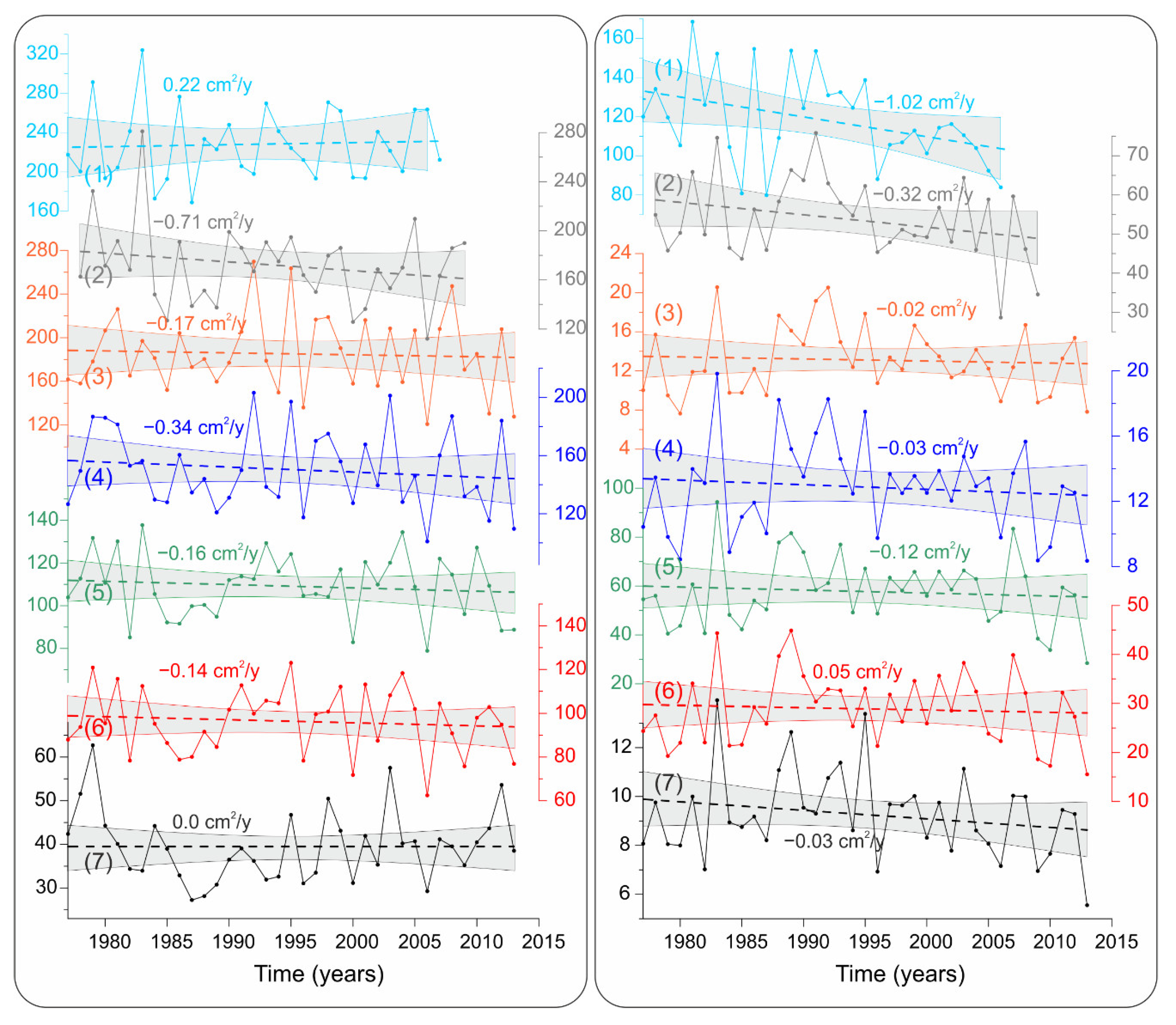
Figure 10.
Wavelet coherence of (a–d) NAO and (e–h) SCAND monthly values with (a,c,e,g) and (b,d,f,h) at (a,b,e,f) Kungsholmsfort and (c,d,g,h) the Gorny Institute. Contours are wavelet squared coherencies. In all panels, the black thin line and the lighter shaded picture show the cone of influence of the edge effects that might distort the coherence.
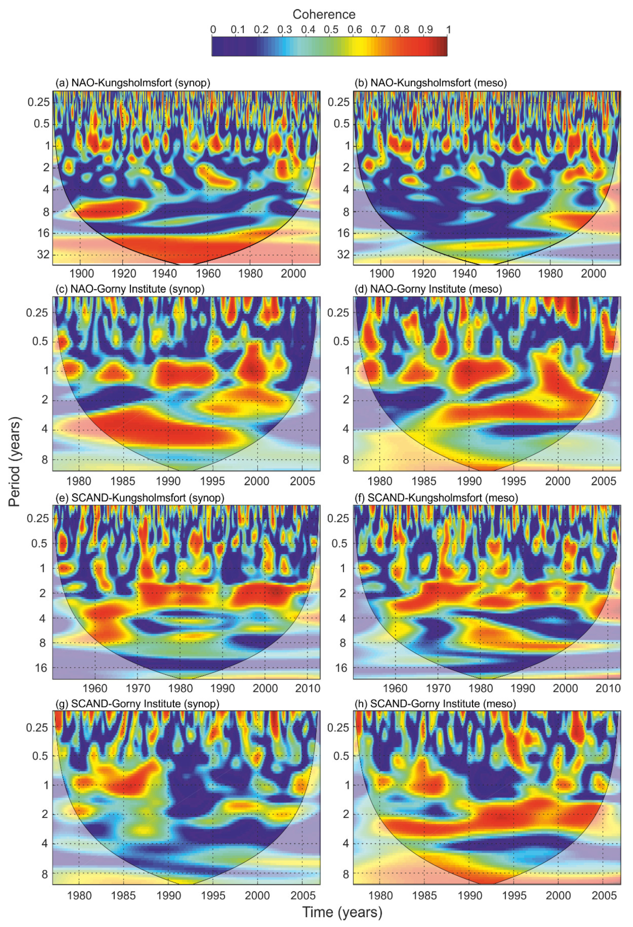
Figure 11.
Wavelet coherence of wind speed from the 20th Century Reanalysis mean monthly values of (a,b,e,f) zonal and (c,d,g,h) meridional components of with (a,c,e,g) , (b,d,f,h) at (a–d) Kungsholmsfort and (e–h) the Gorny Institute. Contours are wavelet squared coherencies. In all panels, the black thin line and the lighter shaded picture shown the cone of influence of the edge effects where might distort the coherence.

Table 1.
The tide gauges which data were used in the study. Numbers in column 1 correspond to stations in Figure 1.
Table 1.
The tide gauges which data were used in the study. Numbers in column 1 correspond to stations in Figure 1.
| No. | Tide Gauge | Longitude (° E) | Latitude (° N) | Observation Period |
|---|---|---|---|---|
| 1 | Gorny Institute | 30.3 | 59.9 | 1977–2007 |
| 2 | Narva | 28.1 | 59.5 | 1978–2009 |
| 3 | Pärnu | 24.5 | 58.4 | 1978–2009 |
| 4 | Ristna | 22.1 | 58.9 | 1978–2009 |
| 5 | Kalix | 23.1 | 65.7 | 1974–2013 |
| 6 | Furuogrund | 21.2 | 64.9 | 1916–2013 |
| 7 | Ratan | 20.9 | 64.0 | 1892–2013 |
| 8 | Stockholm | 18.1 | 59.3 | 1889–2013 |
| 9 | Kungsholmsfort | 15.6 | 56.1 | 1887–2013 |
| 10 | Warnemünde | 12.1 | 54.2 | 1956–2006 |
| 11 | Gedser | 11.9 | 54.6 | 1891–2005 |
| 12 | Klagshamn | 12.9 | 55.5 | 1930–2013 |
Publisher’s Note: MDPI stays neutral with regard to jurisdictional claims in published maps and institutional affiliations. |
© 2021 by the authors. Licensee MDPI, Basel, Switzerland. This article is an open access article distributed under the terms and conditions of the Creative Commons Attribution (CC BY) license (https://creativecommons.org/licenses/by/4.0/).
Share and Cite
MDPI and ACS Style
Medvedev, I.; Medvedeva, A. Seasonal and Decadal Variations of the Variance of the Synoptic and Mesoscale Sea Level Variability in the Baltic Sea. Water 2021, 13, 1785. https://doi.org/10.3390/w13131785
AMA Style
Medvedev I, Medvedeva A. Seasonal and Decadal Variations of the Variance of the Synoptic and Mesoscale Sea Level Variability in the Baltic Sea. Water. 2021; 13(13):1785. https://doi.org/10.3390/w13131785
Chicago/Turabian StyleMedvedev, Igor, and Alisa Medvedeva. 2021. "Seasonal and Decadal Variations of the Variance of the Synoptic and Mesoscale Sea Level Variability in the Baltic Sea" Water 13, no. 13: 1785. https://doi.org/10.3390/w13131785
Note that from the first issue of 2016, this journal uses article numbers instead of page numbers. See further details here.