
Comparison of Forecasting Models for Real-Time Monitoring of Water Quality Parameters Based on Hybrid Deep Learning Neural Networks

1
Tianjin Key Laboratory of Water Resources and Environment, Tianjin Normal University, Tianjin 300387, China
2
State Key Laboratory of Hydro-Science and Engineering, Tsinghua University, Beijing 100084, China
*
Author to whom correspondence should be addressed.
Water 2021, 13(11), 1547; https://doi.org/10.3390/w13111547
Submission received: 12 May 2021
/
Revised: 29 May 2021
/
Accepted: 30 May 2021
/
Published: 31 May 2021
(This article belongs to the Special Issue Machine Learning for Hydro-Systems)
Abstract
:Accurate real-time water quality prediction is of great significance for local environmental managers to deal with upcoming events and emergencies to develop best management practices. In this study, the performances in real-time water quality forecasting based on different deep learning (DL) models with different input data pre-processing methods were compared. There were three popular DL models concerned, including the convolutional neural network (CNN), long short-term memory neural network (LSTM), and hybrid CNN–LSTM. Two types of input data were applied, including the original one-dimensional time series and the two-dimensional grey image based on the complete ensemble empirical mode decomposition algorithm with adaptive noise (CEEMDAN) decomposition. Each type of input data was used in each DL model to forecast the real-time monitoring water quality parameters of dissolved oxygen (DO) and total nitrogen (TN). The results showed that (1) the performances of CNN–LSTM were superior to the standalone model CNN and LSTM; (2) the models used CEEMDAN-based input data performed much better than the models used the original input data, while the improvements for non-periodic parameter TN were much greater than that for periodic parameter DO; and (3) the model accuracies gradually decreased with the increase of prediction steps, while the original input data decayed faster than the CEEMDAN-based input data and the non-periodic parameter TN decayed faster than the periodic parameter DO. Overall, the input data preprocessed by the CEEMDAN method could effectively improve the forecasting performances of deep learning models, and this improvement was especially significant for non-periodic parameters of TN.
1. Introduction
As the most important water source for human life and industry production, surface water is extremely vulnerable to being polluted. By quantifying different types of parameters, water quality monitoring can help us to develop best management practices to protect water source safety and improve aquatic habitats [1]. With the development of the social economy, many regions of China are facing severe water pressure due to increasing water demand and decreasing available water resources as the result of surface water pollution [2]. Therefore, precisely and timely monitoring and prediction of surface water quality is particularly critical to local environmental managers for designing pollution reduction strategies and responding to environmental emergencies. In recent years, many studies have estimated water quality parameters through different methods based on artificial intelligence tools. For example, Fijani et al. designed a hybrid two-layer decomposition using the complete ensemble empirical mode decomposition algorithm with adaptive noise (CEEMDAN) and the variational mode decomposition (VMD) algorithm coupled with extreme learning machines (ELM) to predict chlorophyll-a (Chl-a) and dissolved oxygen (DO) in a reservoir [3]. Chen et al. compared the water quality prediction performances of several machine learning methods using monitoring data from the major rivers and lakes in China from 2012 to 2018 [4]. Lu et al. designed two hybrid decision tree-based models to predict the water quality for the most polluted river Tualatin River in Oregon, USA [5].
Artificial intelligence (AI) techniques have been popular data-based methods in recent years and have been successfully developed to predict nonlinear and non-stationary time series in many fields. For example, the neuro-fuzzy expert systems have been used to monitor the corrosion phenomena in a pulp and paper plant [6]. The artificial neural networks, support vector machine, and adaptive neuro-fuzzy inference systems (ANFIS) were applied to model complex hydrologic systems [7,8]. The fuzzy logic and ANFIS were applied for flood prediction [9]. However, compared to these “shallow” modelling methods, the deep learning (DL) models have been developed as a reliable estimation and prediction tool in many fields, such as image classification [10], speech recognition [11], COVID-19 diagnostic and prognostic analysis [12], rainfall-runoff modeling [12], and streamflow prediction [13]. Among the multiple DL models, long short-term memory (LSTM) and convolutional neural networks (CNN) are the two most commonly used models. Barzegar et al. used standalone LSTM and CNN and hybrid CNN–LSTM models to predict DO and Chl-a in the Small Prespa Lake in Greece, and found that the hybrid model was superior to the standalone models [14]. Hao et al. applied singular spectrum analysis and ensemble empirical mode decomposition to preprocess the data at first, and found that the performances of LSTM model were better than using the raw data directly [15]. Wang et al. used wavelet-based LSTM, CNN–LSTM, and LSTM for monthly streamflow and rainfall forecasting, and found that LSTM was applicable for time series prediction, but the two hybrid models were superior alternatives [16]. The previous studies have shown that the hybrid models are superior to the standalone models, and the preprocessing method could improve the performances of the DL models. However, after analyzing these studies, we think that some issues should be noted and considered. First, different parameters represent different substances, so the time series of these parameters have different fluctuation characteristics. For example, DO is greatly affected by temperature, so it has obvious seasonal variations [17]. The excess total nitrogen (TN) and total phosphorus (TP) entering the surface water mainly comes from human activities, and the seasonal variations are not significant [18]. We wonder whether the DL models have satisfactory prediction performances for different parameters and whether the hybrid models always perform better. Second, the pre-processing method is a data-dependent method, so the model framework gradually becomes unreliable as the data is updated. Evaluating the changes in model performances as time steps increase may help to reduce computational costs. Finally, previous studies generally decomposed the data series first, then predicted each component separately, and then added these prediction results to obtain the reconstructed time series. We think that the calculation process is complicated, and wonder if there is a simplified method to achieve accurate prediction.
In this study, the DL models CNN, LSTM, and CNN–LSTM were used to forecast the real-time monitoring water quality parameters. A dataset that recorded data every four hours from 2015 to 2020 was used for the study, which was collected from Xin’anjiang River, China. The DO and TN were selected as target parameters, and the original time series were used to train and test the standalone and hybrid models. Additionally, the CEEMDAN model was used to decompose the input data, and the decomposition matrices were used as two-dimensional gray images input data as a comparison. The main objectives of this study were to (1) compare the results based on the original input data and the two-dimensional input data and analyze the impact of different input data on the performances of the models; (2) compare the results of standalone and hybrid models with different parameters and analyze the influence of parameter fluctuation characteristics on model performances; and (3) compare the results of different prediction steps and analyze the impact of prediction steps on different parameters and different models.
2. Materials and Methods
2.1. Study Area and Data Description
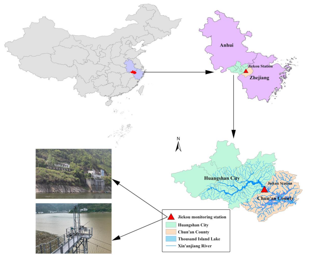
The case study area in this paper is Xin’anjiang River, which is a transboundary river that crosses Anhui Province and Zhejiang Province. The Xin’anjiang River originated in Huangshan City, Anhui Province, and flows into Thousand Island Lake through Chun’an County, Zhejiang Province (Figure 1). As the most important water source flowing into the Thousand Island Lake, the water quality of Xin’anjiang River is concerned with the health of 115.91 million people in both Anhui and Zhejiang provinces [19]. The Jiekou monitoring station is located at the junction of these two provinces, which is mainly used to monitor the water quality of Xin’anjiang River (Figure 1). Jiekou station automatically analyzes water samples and records data every 4 h to realize real-time monitoring of water quality. We collected water quality data including dissolved oxygen (DO) and total nitrogen (TN) from 0:00 on 6 May 2015 to 20:00 on 20 January 2020. The DO and TN datasets both had 10,326 records, which were used to conduct the predictive models. To perform the model development and evaluation, the full dataset was split into training, validating, and testing subsets. The data division criterion in this study was shown in Figure 2. The training, validating, and testing sub-sets included 6609 records (nearly 64% of the dataset, from 0:00 on 6 May 2015 to 8:00 on 11 May 2018), 1652 records (nearly 16% of the dataset, from 12:00 on 11 May 2018 to 20:00 on 10 February 2019), and 2065 records (nearly 20% of the dataset, from 0:00 on 11 February 2019 to 20:00 on 20 January 2020), respectively. The descriptive statistics of the training set, validating set, and testing set for these two parameters were summarized in Table 1.
2.2. Complementary Ensemble Empirical Mode Decomposition with Adaptive Noise
CEEMDAN is an improved adaptive signal time–frequency analysis method [20], which is developed following the empirical mode decomposition (EMD) [21] and ensemble empirical mode decomposition (EEMD) [22]. EMD could decompose complex signal into intrinsic mode functions (IMFs) and a residue, so as to better understand the linear and nonlinear characteristics of the signal. However, since either a single IMF is composed of very different scales, or similar scales reside in different IMF components, the original EMD has the disadvantage of mode mixing [3]. The EEMD method is proposed to solve the problem of mode mixing by adding white noise [22]. However, the added white noise could not be completely eliminated during the decomposition process, so the interaction between the signal and the noise may produce different modes [23]. The CEEMD algorithm completely eliminates the residual white noise by adding positive and negative auxiliary white noise pairs to the original signal, and further improves the performance of the decomposition algorithm [24]. By introducing the adaptive noise component, the CEEMDAN algorithm not only maintains the ability to eliminate mode mixing and residual noise, but also has fewer iterations and higher convergence performance [20]. In this study, CEEMDAN was used to decompose the original DO and TN data series to reduce their complexities.
2.3. Convolutional Neural Network
The convolutional neural network (CNN) is a multi-layer feedforward neural network that can be used to process data of multiple dimensions, such as time series data (which can be considered as a 1-D grid sampled at regular intervals) and image data (which can be considered as pixel 2-D grid) [25]. With the application of CNNs, many variants of convolutional network structure have appeared. However, the basic structures of most networks are similar, including input layer, convolution layer, pooling layer, fully connected layer, and output layer [16,26]. The input data needs to enter the convolutional neural network through the input layer. According to the observed data and study objectives, the input layer has a variety of formats, including 1-D, 2-D, and even n-D, and these data usually contain 1 to n channels. In this study, the original time series could be viewed as 1-D grid data to build a 1-D convolutional network. Moreover, the original data preprocessed by CEEMDAN were decomposed into multi-frequency IMFs, and all of them were put into CNN as input data in the form of image. These images had only one channel, and the CNN built based on them could be considered a 2-D model.
Through a series of comparative experiments, the basic structure of the CNN models used in this study was determined. After the input layer, the second layer was a convolutional layer with a number of learnable convolution kernels. The application of these kernels was to obtain multiple feature maps by learning different features of the input data. The third layer was the activation layer that used rectified linear unit (ReLU) as the activation function. The fourth layer was a pooling layer using the average function. The pooling layer reduced the dimensionality and processing time by sub-sampling the feature maps extracted from the convolutional layer. The fully connected layer, which was the last part before the output layer, connected the output of the pooling layer to a one-dimensional row vector. Finally, for the regression problem of this study, the regression output layer was used as the last layer of CNN. In addition to these basic structures, in order to reduce the problem of overfitting, dropout and batch-normalization methods were used in this study [27]. Dropout randomly set the input elements to zero with a given probability in each training case, so that a large number of different networks could be trained in a reasonable time to effectively reduce the problem of overfitting [28]. Batch normalization can mitigate the internal covariate shift and the dependence of the gradient on the parameter or its initial value, so as to achieve the purpose of accelerating training and producing more reliable models [29].
2.4. Long Short-Term Memory Neural Network
The long short-term memory (LSTM) network is a special variant of the recurrent neural network (RNN). In traditional feedforward neural networks, information can only flow from the input layer to the hidden layer and finally to the output layer in one direction. The biggest difference between RNN and the feedforward neural network is that RNN has a recurrent hidden unit to implicitly maintain historical states about all past elements in the sequence [30,31]. That is to say, in RNN, the final output is based on the feedback of the input layer and the historical states of all hidden units. However, when the RNN is trained using the gradient descent method, the gradient may show an exponential increase or decay, which will cause the gradient to explode or disappear [31,32]. LSTM introduces the concept of input and output gates to improve RNN. LSTM applies memory cells, which could filter and process historical states and information instead of the recurrent hidden units of the RNN, and the basic structure of three consecutive memory cells is shown in Figure 3. Each memory cell contains an input gate (it), a forget gate (ft), and an output gate (Ot) to control the flow of information. The input gate (it) is used to determine how much input data at the current moment (t) needs to be stored in the cell state, and an intermediate value is used to update the state in this process.
The forget gate (ft) determines how much of the cell state from the previous moment (t−1) needs to be retained to the current moment.
By deleting part of the old information and adding the filtered intermediate value, the cell state is updated from Ct−1 to Ct.
The output gate controls how much of the current cell state needs to be output to the new hidden state.
In the above formula, and , respectively, represent the relevant weight matrices and bias vectors, while and are the sigmoid function and hyperbolic tangent function. The basic structure of LSTM models used in this study included the input layer, LSTM layer, fully connected layer, and regression output layer. To prevent overfitting, the dropout layer was inserted before the fully connected layer.
All of the algorithms were performed by programming codes in MATLAB R2020b, and a function developed by Torres et al. [20] was used to design the CEEMDAN model. The Deep Learning Toolbox including the basic framework of multiple deep neural networks was applied to design the CNN, LSTM, and CNN–LSTM models.
2.5. The Hybrid Forecasting Models Development
Before constructing the forecasting models, the Lyapunov exponents were calculated first to determine whether there were nonlinear and dynamic characteristics in the DO and TN data series. When the maximum Lyapunov exponent is positive, it is a powerful indicator of the chaotic features of the data series. The values of the Lyapunov exponent for DO and TN were 0.36 and 0.44, respectively, indicating that the monitoring data of these two parameters were both chaotic time series. For chaotic nonlinear dynamic systems, the data may be corrupted by noise or their internal features may be completely unknown, so deep learning methods are very suitable for prediction and feature extraction of such data. In this study, we investigated the potential uses of single models and hybrid models for multi-step ahead forecasting of DO and TN. The procedures of the water quality prediction models based on CNN and LSTM are described as follows.
Step 1: The explanatory variables and target variable were decided. Although some commonly used analysis methods (such as autocorrelation function and partial autocorrelation function) have been tried to determine the input variables, no significant number of lags has been found. Taking into account the monitoring frequency and effectiveness of the data, twelve records in two days were selected as input variables, and six records in the following day were used as output variables. Taking DO as an example, the input and output variables are shown in Table 2.
Step 2: DO and TN data series were decomposed into several different IMFs and a residual component. These components can provide detailed information from high frequency to low frequency contained in the input data series. Previous studies indicated that the added noise level and the number of realizations in the CEEMDAN modeling process can be adjusted according to the application [33]. According to some empirical algorithms in the previous studies (for example, the recommended white noise amplitude is about 20% of the standard deviation, etc.) and the results of trial and error, a noise level of 0.1, a realization of 100, and a maximum of 2000 sifting iterations were set [3,22,34].
Step 3: The data series were divided into training, validating, and testing sets, respectively. It is worth noting that although the testing subset is completely independent of the training process and is used to compare the forecasting performances of the models, the decomposition process of CEEMDAN needs to be applied to the entire dataset. If the training subset and the testing subset are decomposed separately, the obtained IMFs and residual component are inconsistent and the trained model becomes invalid for the testing data.
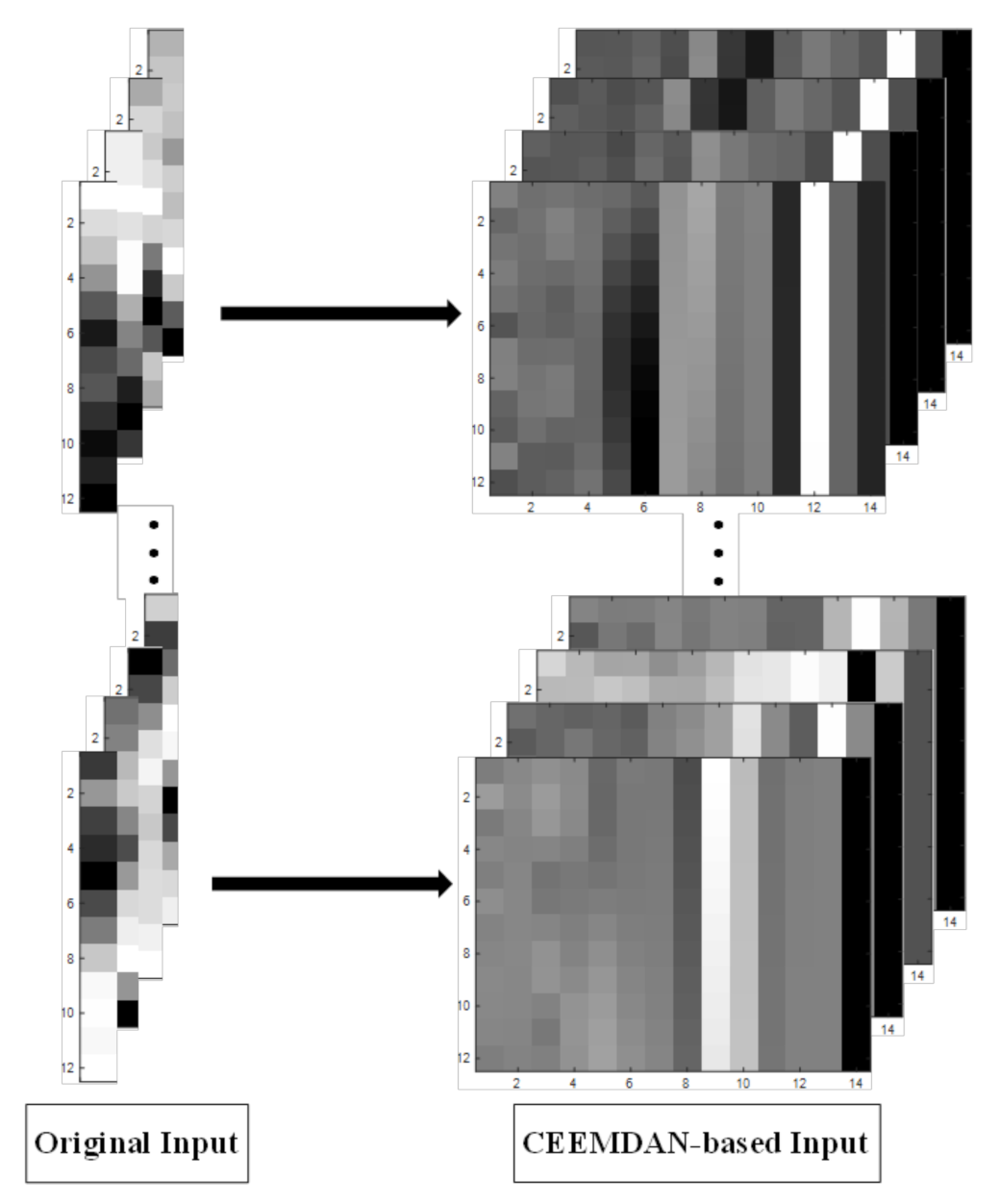
Step 4: The training subset was used to train each model for multi-step ahead forecast. This study contained two types of input data: the original one-dimensional time series and the two-dimensional gray-scale image based on CEEMDAN decomposition. The original one-dimensional input was a set of 12 × 1 data sequences, while the CEEMDAN-based input was a set of 12 × n two-dimensional images (the value of n was decided by the results of decomposition process). The one-dimensional and two-dimensional images are shown in Figure 4, respectively. Each type of data was used to train three deep neural networks: CNN, LSTM, and CNN–LSTM.
Step 5: The testing subset was used to obtain multi-step ahead forecasting results and compare the performances of different models. Since the testing data were not involved in the training process at all, the forecasting results of testing data set could well reflect the generalization ability of the models. At the same time, the results of different ahead steps can be used to evaluate the effective forecasting duration of the models.
2.6. Evaluation Criteria
To quantitatively evaluate the performances of the aforementioned models, three statistical evaluation criteria were selected for comparison, including the coefficient of efficiency (CE), root mean square error (RMSE), and mean absolute percentage error (MAPE). The CE was also known as the Nash–Sutcliffe coefficient and defined as follows:
The RMSE was calculated as:
The MAPE was defined as:
where n was the number of input samples, Oi and Pi were observed and predicted value of sample i, respectively. was the mean value of observed data. Generally, the larger the CE value and the smaller the RMSE and MAPE values, the smaller the difference between the predicted value and the actual value, that is, the higher the prediction accuracy of the model.
3. Results and Discussion
3.1. Results of DO Data Series
Based on the CEEMDAN preprocessing method, the time series of the DO data set were decomposed into 13 IMFs and one residual term, shown in Figure 5. These IMFs reflected the oscillating modes of DO in different periods, and the residual term indicated the trend of the data. In this study, the input data had two forms, one is the original time series, and the other is the gray image based on the CEEMDAN results (Figure 4). The original input was a set of 12 × 1 data sequences, while the CEEMDAN-based input was a set of 12 × 14 two-dimensional images. Obviously, compared to a single time series, the CEEMDAN-based input data could reflect more information. Moreover, increasing the dimensionality of the input data was beneficial to the deep learning neural networks to extract data features, thereby improving the prediction accuracy.
The CE, RMSE, and MAPE statistics of single and hybrid deep learning neural networks in the testing period for the DO dataset are shown in Table 3. For targets with different ahead steps, the best error measures were highlighted in red. According to the results, it can be found that the CEEMDAN–CNN–LSTM model had the best prediction accuracy for all targets. Whether for the separate CNN and LSTM model or the CNN–LSTM hybrid model, the prediction accuracies of CEEMDAN-based input data were better than the original input data. As the forecasting step increased, the accuracy difference between these two sets of input data gradually increased. For example, the differences of CE, RMSE, and MAPE between DOt and DOt+5 for CNN–LSTM and CEEMDAN–CNN–LSTM were 0.09 (|0.97–0.88|), 0.30 (|0.35–0.65|), and 2.61 (|3.06–5.67|) and 0.04 (|0.98–0.94|), 0.22 (|0.26–0.48|), and 2.01 (|2.55–4.56|), respectively. In other words, as the forecasting step increased, the decrease of the prediction accuracy of CEEMDAN-based input data was slower than the original input data.
The six models, especially the CEEMDAN–CNN–LSTM model, could capture the general trend of the testing data series across different forecasting steps. However, it was necessary to evaluate the model accuracy based on the forecasts of the peak and lowest values. In this study, the MAPE between observations and predictions of the 10% lowest and 10% highest values of the testing data was analyzed. Figure 6a,c showed the MAPE of lowest values from Step 1 to 6 based on original and CEEMDAN-based input. The MAPEs of the six models increased as the forecasting step became longer, and the MAPEs based on the original input data were larger than the CEEMDAN-based input. The MAPEs of the CNN models were the largest, LSTM models were the second, and CNN–LSTM models were the smallest, which indicated that the CNN–LSTM model was superior to the separate models in forecasting the lowest values. For the prediction of peak values (Figure 6b,d), the MAPEs of CEEMDAN-based inputs were smaller than the original inputs, and the MAPEs increased as the forecasting step became longer. Being different from the lowest values prediction, LSTM was the model with the largest MAPEs for the peak values prediction, followed by the CNN model, and CNN–LSTM was the smallest. Therefore, the CEEMDAN–CNN–LSTM was the best forecasting model for both the lowest and highest values.
3.2. Results of TN Data Series
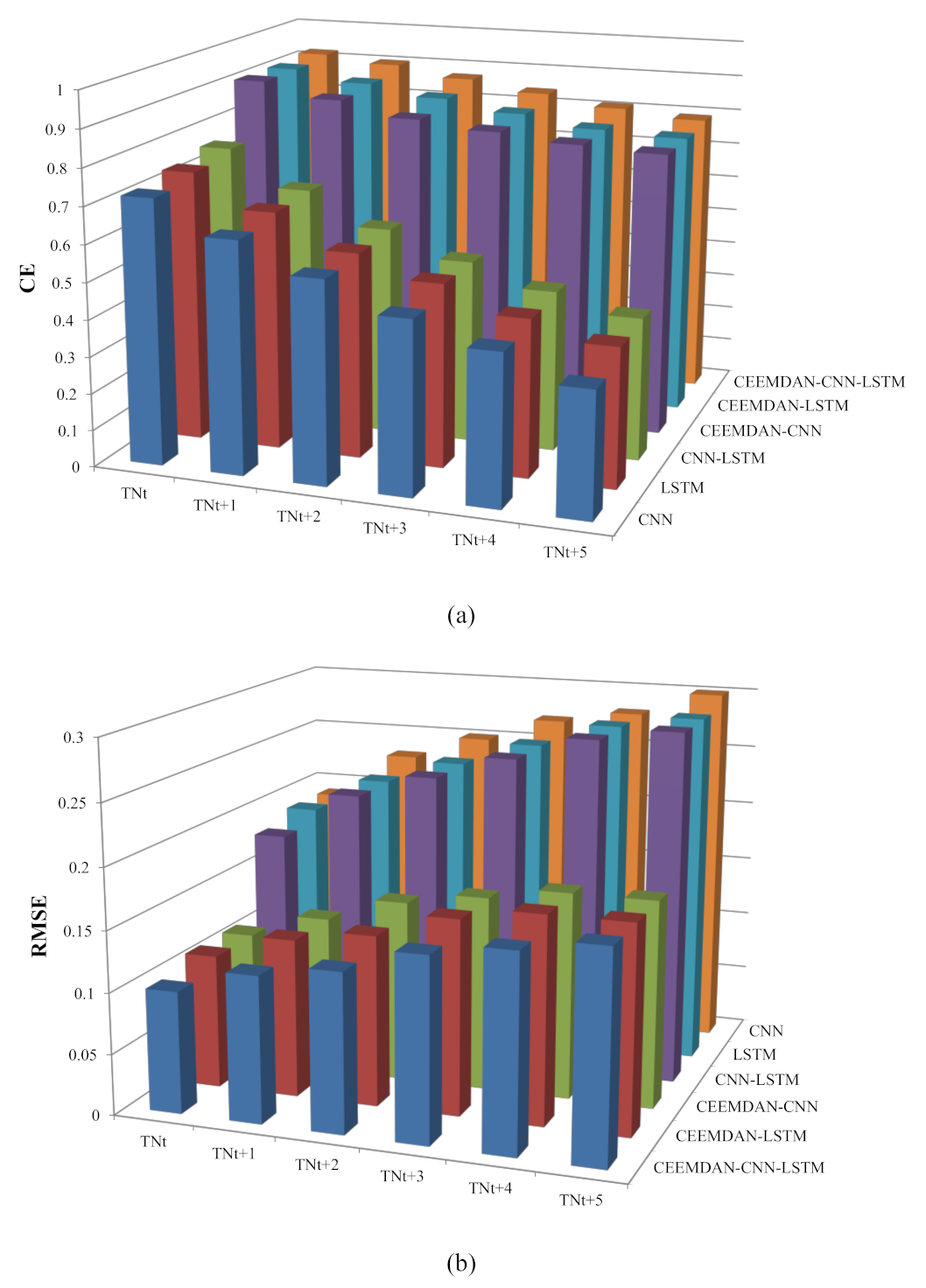
The decomposition results of the TN data series using the CEEMDAN method are shown in Figure 7. The TN data set was also decomposed into 13 IMFs and one residual term. The CE, RMSE, and MAPE statistics of single and hybrid deep learning neural networks in the testing period for the TN dataset are shown in Table 4. The results indicated that the CEEMDAN–CNN–LSTM model had the best performances across different forecasting steps. However, for the prediction of TN, the differences between the results obtained from the original input and the CEEMDAN-based input were very significant. Especially with the increase of the time steps, the performance of the original input deteriorated rapidly, while the CEEMDAN-based input showed much better stability for TN forecasting. For CNN, LSTM, and CNN–LSTM models, the CEs of TNn+3, TNn+4, and TNn+5 were all less than 0.5, which was not within the range of satisfactory model simulations [35]. In other words, when the time step exceeded 3, no model could reliably predict the TN concentration based on the time series data alone.
The MAPEs of different models for the 10% peak values and 10% lowest values of the TN testing data set are shown in Figure 8. The prediction of the lowest values showed that the CNN–LSTM was better than the CNN, while the LSTM performed the worst among the three models (Figure 8a,c). For the original input and CEEMDAN-based input, the average MAPEs of the three models across different time steps were 39.20, 41.71, and 51.72 and 26.07, 28.12, and 31.30, respectively. Obviously, the prediction of the lowest values based on the original input data had a greater deviation from the observed values. According to the prediction results of the peak values, LSTM was the worst performing model, followed by the CNN model, and the CNN–LSTM model performed best (Figure 8b,d). In addition, as the time step increased, the MAPEs gradually became larger, that is, the deviation between the predicted values and the observed values became larger. The change curves of MAPE were nearly the same; however, the MAPEs obtained from the original input were about twice the MAPEs obtained from the CEEMDAN-based input. In general, CEEMDAN–CNN–LSTM was the best model for forecasting TN extreme values, while LSTM was the least accurate model for extreme values prediction.
4. Discussion
Numerous studies have applied single and hybrid deep learning models to predict hydrological and water quality data [15,16,36]. Among them, the most commonly used method was to decompose the data series at first, then make predictions for each IMF separately, and finally add the results to get the reconstructed time series. However, data decomposition was a data-dependent method, so it needed to be repeated as the data was updated. Generally, huge calculation cost was accompanied by long calculation time, so the commonly used method was too time-consuming for real-time data prediction. In this study, we tried to input the decomposed data series as two-dimensional images for multi-step water quality prediction. The results indicated that compared with the original one-dimensional time series input data, the two-dimensional input data decomposed by the CEEMDAN method could improve the prediction accuracies. However, for water quality parameters with different fluctuation characteristics, the two-dimensional input data improved the prediction accuracies differently. It can be found from Figure 4 that the DO data had very obvious seasonal changes. The DO concentrations in spring and summer were higher than those in autumn and winter. Due to the strong periodicity of DO data, the standalone model and hybrid model with two types of input data had satisfactory performances. However, the performances of the hybrid models were slightly better than that of the standalone models, so the results were compared and discussed based on the hybrid models. For DOt, the CE, RMSE, and MAPE of CNN–LSTM and CEEMDAN–CNN–LSTM were 0.97 vs. 0.98, 0.35 vs. 0.26, and 3.06 vs. 2.55, respectively. The performance of the CEEMDAN–CNN–LSTM model was better, but the CNN–LSTM model could also capture the fluctuation characteristics of the data and make accurate predictions. Figure 7 showed that the TN data, which was mainly affected by human activities, had no periodic fluctuation characteristics. The results based on the CEEMDAN input data were significantly better than the results based on the original input data. For TNt, the CE, RMSE, and MAPE of CNN–LSTM and CEEMDAN–CNN–LSTM were 0.76 vs. 0.92, 0.18 vs. 0.10, and 10.06 vs. 6.63, respectively. The CEEMDAN–CNN–LSTM model performed significantly better than the CNN–LSTM, which indicated that decomposing the input data was more beneficial to improve the prediction accuracy of non-periodic time series. The CEEMDAN method added adaptive white noise in each decomposition to smooth the impulse interference, so that the decomposition of the data was very complete [37]. For non-periodic parameters, the complete decomposition could better separate the noise component and periodic components of the data. Among them, the periodic components could be much better predicted, so the prediction accuracies of the data series were also improved.
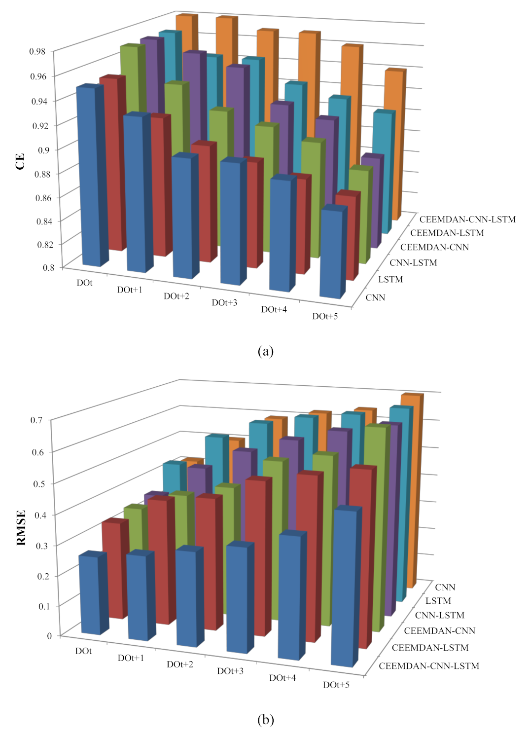
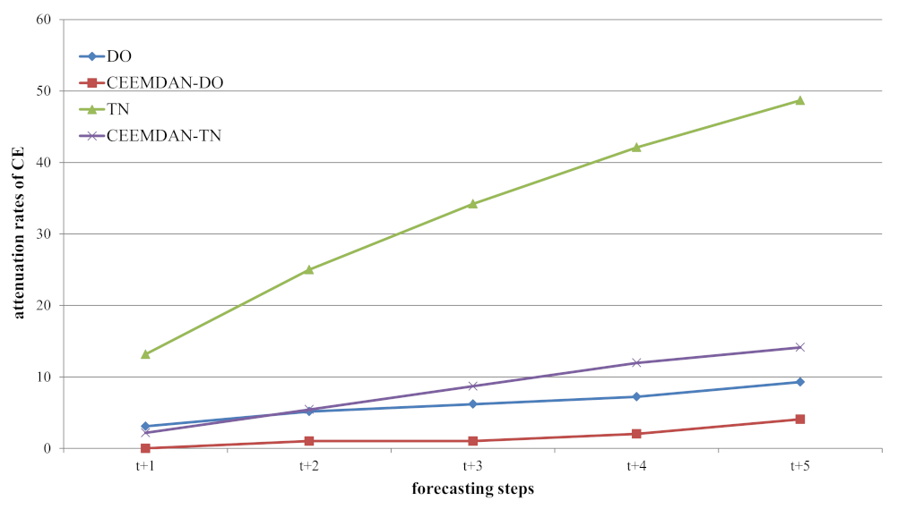
Increasing the forecasting steps of each round of prediction may help to reduce computational consumption, while relevant previous studies rarely discussed the impact of the increase in forecasting steps on model performances [14,15]. In this study, all of the models were tested for one-step-ahead (4 h) to six-step-ahead (1 day) forecasting, which were aimed to analyze the impact of the forecasting steps on the performances of the models. As shown in Figure 9 and Figure 10, with the increase of prediction steps, the CE of all models decreased, while the RMSE and MAPE gradually increased. Some previous studies on hydrological data prediction have also obtained similar results on a monthly scale. For example, in a wavelet analysis–ANN-model-based multi-scale monthly groundwater level prediction study, the prediction results of 2 and 3 months ahead were worse than the results of 1 month ahead [38]. In the study using a two-phase hybrid model to predict the runoff in Yingluoxia watershed, the model’s accuracy for shorter lead times (1 month) were better than the 3- and 6-month horizon [34]. However, in addition to the conclusion that the prediction accuracy would decrease with the increase of prediction steps, we found that the accuracies’ attenuation rates of different water quality parameters were different. Taking the indicator CE as an example, the CE attenuation rates of the DO models were much lower than those of the TN models as the prediction steps increased. Based on the CE at time t (i.e., one-step-ahead), the CE attenuation rates of CNN–LSTM and CEEMDAN–CNN–LSTM models at time t+1, t+2, t+3, t+4, and t+5 were calculated, and the results are shown in Figure 11. For DO, the attenuation rates of CNN–LSTM models and CEEMDAN–CNN–LSTM models were 3.09~9.28 and 0~4.08, respectively. For TN, the attenuation rates of CNN–LSTM models and CEEMDAN–CNN–LSTM models were 13.16~48.68 and 2.17~14.13, respectively. Obviously, the attenuation rates of the periodic parameter DO were lower than those of the non-periodic parameter TN, and the attenuation rates based on two-dimensional input data were lower than those of one-dimensional input data. It was interesting to note that the prediction accuracy decreased as the number of prediction steps increased. With the continuous flow of the river, the waters that have experienced different influences gradually flowed through the monitoring station. As the time interval became longer, the differences of water quality became greater. Therefore, the prediction accuracies based on the same set of input data gradually decreased. Moreover, the TN concentrations were mainly affected by human activities. The TN emission sources were always changing, as the prediction steps increased, the sources may appear or disappear. Therefore, the attenuation rates of TN were faster than DO.
5. Conclusions
In this study, the performances of the deep neural networks CNN, LSTM, and CNN–LSTM with and without the preprocessing method CEEMDAN were compared for the water quality parameters’ forecasting. A real-time water quality monitoring dataset with 10,326 records from 2015 to 2020 was collected as the input data. According to the completeness of the data and the fluctuation characteristics of the parameters, DO and TN were selected as prediction targets. The DO and TN data series were decomposed by the CEEMDAN method at first, and two decomposed datasets with 13 IMFs and one residual term were obtained. Taking into account the monitoring frequency (every 4 h) of the data, twelve records in two days were selected as input variables, and six records in the following day were used as output variables. Then, a set of 12 × 1 data sequences was prepared as the original input data, while the CEEMDAN-based input data were a set of 12 × 14 two-dimensional grey images. The two types of input data were used to train and test CNN, LSTM, and CNN–LSTM models, respectively. The results indicated that the performances of hybrid model CNN–LSTM were superior to the standalone model CNN and LSTM. The models used CEEMDAN-based two-dimensional input data performed much better than the models used the original input data. Moreover, the improvements of CEEMDAN-based data for non-periodic parameter TN were much greater than that for periodic parameter DO. In addition, the impacts of the prediction steps on the forecasting accuracies of the models were analyzed in this study. The results showed that the model forecasting accuracies gradually decreased with the increase of prediction steps. The attenuation rates presented the features that the original input data decayed faster than the CEEMDAN-based input data and the non-periodic parameter TN decayed faster than the periodic parameter DO. In general, the input data preprocessed by the CEEMDAN method could effectively improve the forecasting performances of deep neural networks, and this improvement was especially obvious for non-periodic parameter. Overall, compared with a separate monitoring system, the incorporated monitoring and modeling framework may provide better knowledge, which could help decision-making departments respond to upcoming events and outbreaks.
Author Contributions
Conceptualization, J.S.; data curation, J.S. and M.Z.; funding acquisition, X.L.; methodology, X.L.; writing—original draft, J.S.; writing—review and editing, X.L. and Z.-L.W. All authors have read and agreed to the published version of the manuscript.
Funding
This research was funded by National Natural Science Foundation of China, No. 41372373, the innovation team training plan of the Tianjin Education Committee, TD12-5037, and the Science and Technology Development Fund of Tianjin Education Commission for Higher Education, 2018KJ160.
Institutional Review Board Statement
Not applicable.
Informed Consent Statement
Not applicable.
Data Availability Statement
Restrictions apply to the availability of these data. Data were obtained from Ministry of Ecology and Environment of the People’s Republic of China and are available at http://106.37.208.243:8068/GJZ/Business/Publish/Main.html, accessed on 21 April 2021.
Acknowledgments
The authors would like to thank the Ministry of Ecology and Environment of the People’s Republic of China and the Huangshan Ecology and Environment Monitoring Station for the data support. The authors also would like to acknowledgement for the basic background data support from “National Geographic Resource Science SubCenter, National Earth System Science Data Center, National Science & Technology Infrastructure of China (http://gre.geodata.cn)” and China Meteorological Data Service Centre (http://data.cma.cn).
Conflicts of Interest
The authors declare no conflict of interest.
References
- Jiang, J.; Tang, S.; Han, D.; Fu, G.; Solomatine, D.; Zheng, Y. A comprehensive review on the design and optimization of surface water quality monitoring networks. Environ. Model. Softw. 2020, 132, 104792. [Google Scholar] [CrossRef]
- Sun, Y.; Chen, Z.; Wu, G.; Wu, Q.; Zhang, F.; Niu, Z.; Hu, H.-Y. Characteristics of water quality of municipal wastewater treatment plants in China: Implications for resources utilization and management. J. Clean. Prod. 2016, 131, 1–9. [Google Scholar] [CrossRef] [Green Version]
- Fijani, E.; Barzegar, R.; Deo, R.; Tziritis, E.; Skordas, K. Design and implementation of a hybrid model based on two-layer decomposition method coupled with extreme learning machines to support real-time environmental monitoring of water quality parameters. Sci. Total Environ. 2019, 648, 839–853. [Google Scholar] [CrossRef]
- Chen, K.; Chen, H.; Zhou, C.; Huang, Y.; Qi, X.; Shen, R.; Liu, F.; Zuo, M.; Zou, X.; Wang, J. Comparative analysis of surface water quality prediction performance and identification of key water parameters using different machine learning models based on big data. Water Res. 2020, 171, 115454. [Google Scholar] [CrossRef] [PubMed]
- Lu, H.; Ma, X. Hybrid decision tree-based machine learning models for short-term water quality prediction. Chemosphere 2020, 249, 126169. [Google Scholar] [CrossRef] [PubMed]
- Bucolo, M.; Fortuna, L.; Nelke, M.; Rizzo, A.; Sciacca, T. Prediction models for the corrosion phenomena in Pulp & Paper plant. Control Eng. Pract. 2002, 10, 227–237. [Google Scholar]
- Li, X.; Sha, J.; Li, Y.-M.; Wang, Z.-L. Comparison of hybrid models for daily streamflow prediction in a forested basin. J. Hydroinform. 2018, 20, 191–205. [Google Scholar] [CrossRef] [Green Version]
- Mohammadi, B.; Linh, N.T.T.; Pham, Q.B.; Ahmed, A.N.; Vojteková, J.; Guan, Y.; Abba, S.; El-Shafie, A. Adaptive neuro-fuzzy inference system coupled with shuffled frog leaping algorithm for predicting river streamflow time series. Hydrol. Sci. J. 2020, 65, 1738–1751. [Google Scholar] [CrossRef]
- Tabbussum, R.; Dar, A.Q. Performance evaluation of artificial intelligence paradigms—artificial neural networks, fuzzy logic, and adaptive neuro-fuzzy inference system for flood prediction. Environ. Sci. Pollut. Res. 2021, 1–18. [Google Scholar] [CrossRef]
- Raj, R.J.S.; Shobana, S.J.; Pustokhina, I.V.; Pustokhin, D.A.; Gupta, D.; Shankar, K. Optimal feature selection-based medical image classification using deep learning model in internet of medical things. IEEE Access 2020, 8, 58006–58017. [Google Scholar] [CrossRef]
- Jin, Y.; Wen, B.; Gu, Z.; Jiang, X.; Shu, X.; Zeng, Z.; Zhang, Y.; Guo, Z.; Chen, Y.; Zheng, T. Deep-Learning-Enabled MXene-Based Artificial Throat: Toward Sound Detection and Speech Recognition. Adv. Mater. Technol. 2020, 5, 2000262. [Google Scholar] [CrossRef]
- Wang, S.; Zha, Y.; Li, W.; Wu, Q.; Li, X.; Niu, M.; Wang, M.; Qiu, X.; Li, H.; Yu, H. A fully automatic deep learning system for COVID-19 diagnostic and prognostic analysis. Eur. Respir. J. 2020, 56. [Google Scholar] [CrossRef] [PubMed]
- Xiang, Z.; Demir, I. Distributed long-term hourly streamflow predictions using deep learning—A case study for State of Iowa. Environ. Model. Softw. 2020, 131, 104761. [Google Scholar] [CrossRef]
- Barzegar, R.; Aalami, M.T.; Adamowski, J. Short-term water quality variable prediction using a hybrid CNN–LSTM deep learning model. Stoch. Environ. Res. Risk Assess. 2020, 34, 415–433. [Google Scholar] [CrossRef]
- An, L.; Hao, Y.; Yeh, T.-C.J.; Liu, Y.; Liu, W.; Zhang, B. Simulation of karst spring discharge using a combination of time–frequency analysis methods and long short-term memory neural networks. J. Hydrol. 2020, 589, 125320. [Google Scholar] [CrossRef]
- Ni, L.; Wang, D.; Singh, V.P.; Wu, J.; Wang, Y.; Tao, Y.; Zhang, J. Streamflow and rainfall forecasting by two long short-term memory-based models. J. Hydrol. 2020, 583, 124296. [Google Scholar] [CrossRef]
- Liu, G.; He, W.; Cai, S. Seasonal Variation of Dissolved Oxygen in the Southeast of the Pearl River Estuary. Water 2020, 12, 2475. [Google Scholar] [CrossRef]
- Zhang, X.; Yi, Y.; Yang, Z. Nitrogen and phosphorus retention budgets of a semiarid plain basin under different human activity intensity. Sci. Total Environ. 2020, 703, 134813. [Google Scholar] [CrossRef]
- Li, X.; Feng, J.; Wellen, C.; Wang, Y. A Bayesian approach of high impaired river reaches identification and total nitrogen load estimation in a sparsely monitored basin. Environ. Sci. Pollut. Res. 2017, 24, 987–996. [Google Scholar] [CrossRef]
- Torres, M.E.; Colominas, M.A.; Schlotthauer, G.; Flandrin, P. A complete ensemble empirical mode decomposition with adaptive noise. In Proceedings of the 2011 IEEE International Conference on Acoustics, Speech and Signal Processing (ICASSP), Prague, Czech Republic, 22–27 May 2011; pp. 4144–4147. [Google Scholar]
- Huang, N.E.; Shen, Z.; Long, S.R.; Wu, M.C.; Shih, H.H.; Zheng, Q.; Yen, N.-C.; Tung, C.C.; Liu, H.H. The empirical mode decomposition and the Hilbert spectrum for nonlinear and non-stationary time series analysis. Proc. R. Soc. Lond. Ser. A Math. Phys. Eng. Sci. 1998, 454, 903–995. [Google Scholar] [CrossRef]
- Wu, Z.; Huang, N.E. Ensemble empirical mode decomposition: A noise-assisted data analysis method. Adv. Adapt. Data Anal. 2009, 1, 1–41. [Google Scholar] [CrossRef]
- Rahimpour, A.; Amanollahi, J.; Tzanis, C.G. Air quality data series estimation based on machine learning approaches for urban environments. Air Qual. Atmos. Health 2021, 14, 191–201. [Google Scholar] [CrossRef]
- Yeh, J.-R.; Shieh, J.-S.; Huang, N.E. Complementary ensemble empirical mode decomposition: A novel noise enhanced data analysis method. Adv. Adapt. Data Anal. 2010, 2, 135–156. [Google Scholar] [CrossRef]
- Harbola, S.; Coors, V. One dimensional convolutional neural network architectures for wind prediction. Energy Convers. Manag. 2019, 195, 70–75. [Google Scholar] [CrossRef]
- Wang, H.-Z.; Li, G.-Q.; Wang, G.-B.; Peng, J.-C.; Jiang, H.; Liu, Y.-T. Deep learning based ensemble approach for probabilistic wind power forecasting. Appl. Energy 2017, 188, 56–70. [Google Scholar] [CrossRef]
- Miao, Q.; Pan, B.; Wang, H.; Hsu, K.; Sorooshian, S. Improving monsoon precipitation prediction using combined convolutional and long short term memory neural network. Water 2019, 11, 977. [Google Scholar] [CrossRef] [Green Version]
- Hinton, G.E.; Srivastava, N.; Krizhevsky, A.; Sutskever, I.; Salakhutdinov, R.R. Improving neural networks by preventing co-adaptation of feature detectors. arXiv 2012, arXiv:1207.0580. [Google Scholar]
- Ioffe, S.; Szegedy, C. Batch normalization: Accelerating deep network training by reducing internal covariate shift. arXiv 2015, arXiv:1502.03167. [Google Scholar]
- Wang, K.; Qi, X.; Liu, H. A comparison of day-ahead photovoltaic power forecasting models based on deep learning neural network. Appl. Energy 2019, 251, 113315. [Google Scholar] [CrossRef]
- LeCun, Y.; Bengio, Y.; Hinton, G. Deep learning. Nature 2015, 521, 436–444. [Google Scholar] [CrossRef]
- Niu, H.; Xu, K.; Wang, W. A hybrid stock price index forecasting model based on variational mode decomposition and LSTM network. Appl. Intell. 2020, 50, 4296–4309. [Google Scholar] [CrossRef]
- Al-Musaylh, M.S.; Deo, R.C.; Li, Y.; Adamowski, J.F. Two-phase particle swarm optimized-support vector regression hybrid model integrated with improved empirical mode decomposition with adaptive noise for multiple-horizon electricity demand forecasting. Appl. Energy 2018, 217, 422–439. [Google Scholar] [CrossRef]
- Wen, X.; Feng, Q.; Deo, R.C.; Wu, M.; Yin, Z.; Yang, L.; Singh, V.P. Two-phase extreme learning machines integrated with the complete ensemble empirical mode decomposition with adaptive noise algorithm for multi-scale runoff prediction problems. J. Hydrol. 2019, 570, 167–184. [Google Scholar] [CrossRef]
- Moriasi, D.N.; Arnold, J.G.; Van Liew, M.W.; Bingner, R.L.; Harmel, R.D.; Veith, T.L. Model evaluation guidelines for systematic quantification of accuracy in watershed simulations. Trans. ASABE 2007, 50, 885–900. [Google Scholar] [CrossRef]
- Yu, Z.; Yang, K.; Luo, Y.; Shang, C. Spatial-temporal process simulation and prediction of chlorophyll-a concentration in Dianchi Lake based on wavelet analysis and long-short term memory network. J. Hydrol. 2020, 582, 124488. [Google Scholar] [CrossRef]
- Dai, S.; Niu, D.; Li, Y. Daily peak load forecasting based on complete ensemble empirical mode decomposition with adaptive noise and support vector machine optimized by modified grey wolf optimization algorithm. Energies 2018, 11, 163. [Google Scholar] [CrossRef] [Green Version]
- Wen, X.; Feng, Q.; Deo, R.C.; Wu, M.; Si, J. Wavelet analysis–artificial neural network conjunction models for multi-scale monthly groundwater level predicting in an arid inland river basin, northwestern China. Hydrol. Res. 2017, 48, 1710–1729. [Google Scholar] [CrossRef]
Figure 1.
Location of the Jiekou monitoring station.

Figure 2.
The data division criteria in this study.
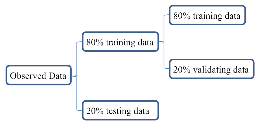
Figure 3.
The architecture of long short-term memory (LSTM) neural network.
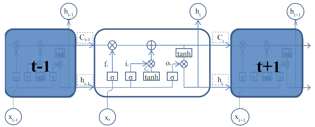
Figure 4.
The two types of input data used in this study.

Figure 5.
The original DO time series, and IMFs and the residual components decomposed by the CEEMDAN method.
Figure 5.
The original DO time series, and IMFs and the residual components decomposed by the CEEMDAN method.
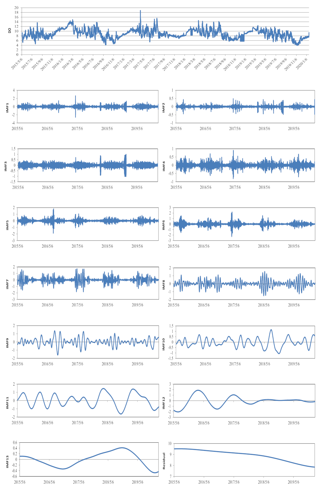
Figure 6.
The MAPE between observations and predictions of the 10% lowest and 10% highest values of the DO testing data: (a) the MAPE of lowest values from step 1 to 6 based on original input data, (b) the MAPE of peak values from step 1 to 6 based on original input data, (c) the MAPE of lowest values from step 1 to 6 based on CEEMDAN input data, and (d) the MAPE of peaks values from step 1 to 6 based on CEEMDAN input data.
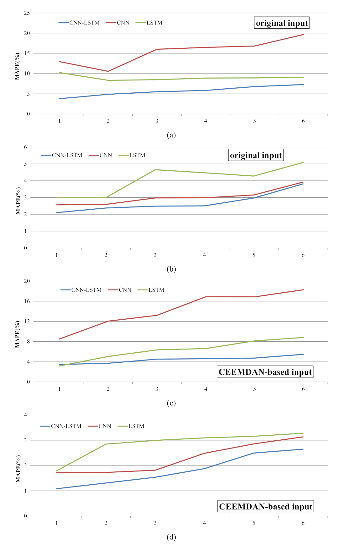
Figure 7.
The original TN time series, and IMFs and the residual components decomposed by the CEEMDAN method.
Figure 7.
The original TN time series, and IMFs and the residual components decomposed by the CEEMDAN method.
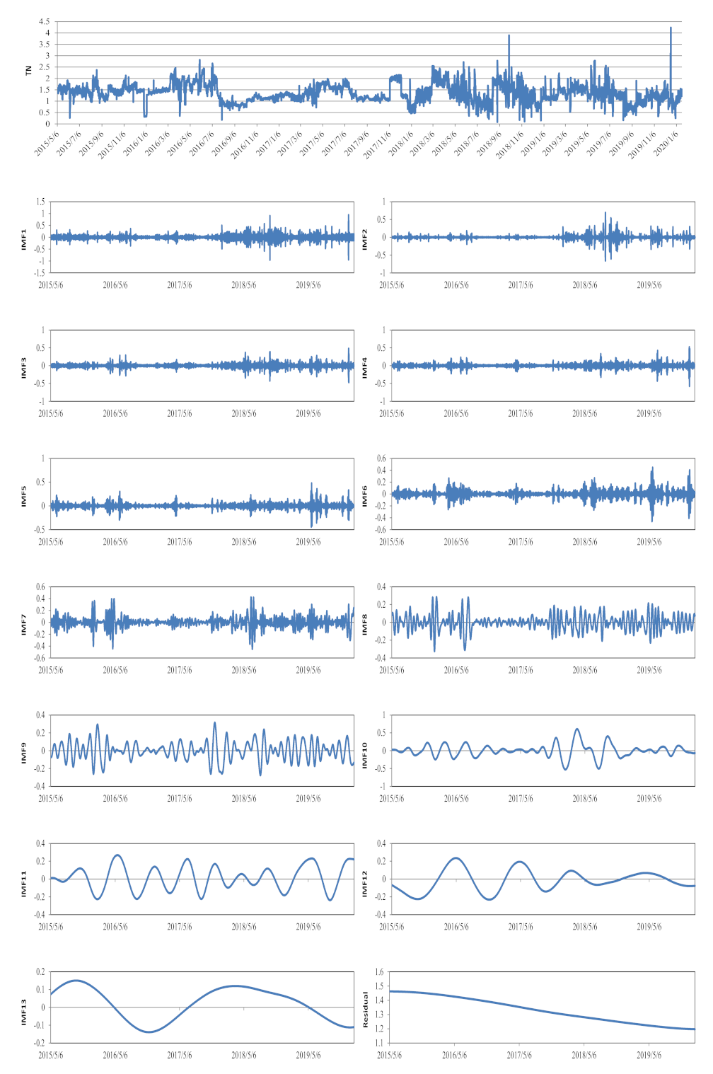
Figure 8.
The MAPE between observations and predictions of the 10% lowest and 10% highest values of the TN testing data: (a) the MAPE of lowest values from Step 1 to 6 based on original input data, (b) the MAPE of peak values from Step 1 to 6 based on original input data, (c) the MAPE of lowest values from Step 1 to 6 based on CEEMDAN input data, (d) the MAPE of peaks values from Step 1 to 6 based on CEEMDAN input data.

Figure 9.
The variations of different models’ performances for DO with the increase of prediction steps: (a) CE, (b) RMSE.
Figure 9.
The variations of different models’ performances for DO with the increase of prediction steps: (a) CE, (b) RMSE.

Figure 10.
The variations of different models’ performances for TN with the increase of prediction steps: (a) CE, (b) RMSE.
Figure 10.
The variations of different models’ performances for TN with the increase of prediction steps: (a) CE, (b) RMSE.

Figure 11.
The CE attenuation rates of CNN–LSTM and CEEMDAN–CNN–LSTM models from Step 1 to 6 for DO and TN.
Figure 11.
The CE attenuation rates of CNN–LSTM and CEEMDAN–CNN–LSTM models from Step 1 to 6 for DO and TN.


Table 1.
Descriptive statistics of training, validating, and testing datasets for DO and TN.
| Descriptive Statistics | Unit | DO | TN | ||||
|---|---|---|---|---|---|---|---|
| T 1 | V 2 | T 3 | T 1 | V 2 | T 3 | ||
| Min. | mg/L | 4.12 | 5.7 | 3.95 | 0.18 | 0.08 | 0.16 |
| Mean | mg/L | 9.13 | 8.5 | 8.18 | 1.4 | 1.24 | 1.24 |
| Median | mg/L | 8.87 | 8.39 | 8.15 | 1.38 | 1.15 | 1.26 |
| Max. | mg/L | 18.85 | 14.14 | 12.42 | 2.82 | 3.9 | 4.24 |
| Standard deviation | mg/L | 1.79 | 1.69 | 1.91 | 0.37 | 0.42 | 0.37 |
| Skewness | dimensionless | 0.41 | 0.49 | −0.2 | 0.2 | 0.478 | 0.85 |
| Kurtosis | dimensionless | 0.27 | −0.25 | −0.8 | 0.12 | 0.61 | 0.36 |
1 Training datasets. 2 Validating datasets. 3 Testing datasets.
Table 2.
Input matrix for the DO forecasting models.
| Target | Input1 | Input2 | Input3 | … | Input 11 | Input 12 |
|---|---|---|---|---|---|---|
| DOt | DOt−1 | DOt−2 | DOt−3 | … | DOt−11 | DOt−12 |
| DOt+1 | DOt−1 | DOt−2 | DOt−3 | … | DOt−11 | DOt−12 |
| DOt+2 | DOt−1 | DOt−2 | DOt−3 | … | DOt−11 | DOt−12 |
| DOt+3 | DOt−1 | DOt−2 | DOt−3 | … | DOt−11 | DOt−12 |
| DOt+4 | DOt−1 | DOt−2 | DOt−3 | … | DOt−11 | DOt−12 |
| DOt+5 | DOt−1 | DOt−2 | DOt−3 | … | DOt−11 | DOt−12 |
Table 3.
The performance statistics of CNN, LSTM, CNN–LSTM, CEEMDAN–CNN, CEEMDAN–LSTM, and CEEMDAN–CNN–LSTM in the testing period for the DO dataset.
Table 3.
The performance statistics of CNN, LSTM, CNN–LSTM, CEEMDAN–CNN, CEEMDAN–LSTM, and CEEMDAN–CNN–LSTM in the testing period for the DO dataset.
| Target | Models | CE | RMSE | MAPE |
|---|---|---|---|---|
| DOt | CNN | 0.95 | 0.41 | 4.17 |
| LSTM | 0.95 | 0.43 | 4.29 | |
| CNN–LSTM | 0.97 | 0.35 | 3.06 | |
| CEEMDAN–CNN | 0.97 | 0.34 | 4.02 | |
| CEEMDAN–LSTM | 0.97 | 0.33 | 3.23 | |
| CEEMDAN–CNN–LSTM | 0.98 | 0.26 | 2.55 | |
| DOt+1 | CNN | 0.93 | 0.50 | 4.68 |
| LSTM | 0.92 | 0.54 | 5.13 | |
| CNN–LSTM | 0.94 | 0.46 | 4.06 | |
| CEEMDAN–CNN | 0.96 | 0.40 | 4.92 | |
| CEEMDAN–LSTM | 0.95 | 0.42 | 4.32 | |
| CEEMDAN–CNN–LSTM | 0.98 | 0.28 | 2.79 | |
| DOt+2 | CNN | 0.90 | 0.59 | 6.03 |
| LSTM | 0.90 | 0.60 | 5.68 | |
| CNN–LSTM | 0.92 | 0.53 | 4.65 | |
| CEEMDAN–CNN | 0.95 | 0.44 | 5.37 | |
| CEEMDAN–LSTM | 0.95 | 0.44 | 4.62 | |
| CEEMDAN–CNN–LSTM | 0.97 | 0.31 | 3.00 | |
| DOt+3 | CNN | 0.90 | 0.62 | 6.21 |
| LSTM | 0.89 | 0.63 | 5.87 | |
| CNN–LSTM | 0.91 | 0.58 | 5.14 | |
| CEEMDAN–CNN | 0.92 | 0.54 | 6.66 | |
| CEEMDAN–LSTM | 0.93 | 0.51 | 5.24 | |
| CEEMDAN–CNN–LSTM | 0.97 | 0.34 | 3.30 | |
| DOt+4 | CNN | 0.89 | 0.64 | 6.34 |
| LSTM | 0.88 | 0.65 | 5.94 | |
| CNN–LSTM | 0.90 | 0.62 | 5.42 | |
| CEEMDAN–CNN | 0.91 | 0.57 | 7.02 | |
| CEEMDAN–LSTM | 0.92 | 0.54 | 5.76 | |
| CEEMDAN–CNN–LSTM | 0.96 | 0.39 | 3.65 | |
| DOt+5 | CNN | 0.87 | 0.70 | 6.96 |
| LSTM | 0.87 | 0.68 | 5.96 | |
| CNN–LSTM | 0.88 | 0.65 | 5.67 | |
| CEEMDAN–CNN | 0.88 | 0.67 | 8.38 | |
| CEEMDAN–LSTM | 0.91 | 0.57 | 6.24 | |
| CEEMDAN–CNN–LSTM | 0.94 | 0.48 | 4.56 |
Table 4.
The performance statistics of CNN, LSTM, CNN–LSTM, CEEMDAN–CNN, CEEMDAN–LSTM, and CEEMDAN–CNN–LSTM in the testing period for the TN dataset.
Table 4.
The performance statistics of CNN, LSTM, CNN–LSTM, CEEMDAN–CNN, CEEMDAN–LSTM, and CEEMDAN–CNN–LSTM in the testing period for the TN dataset.
| Target | Models | CE | RMSE | MAPE |
|---|---|---|---|---|
| TNt | CNN | 0.72 | 0.19 | 10.79 |
| LSTM | 0.74 | 0.19 | 11.21 | |
| CNN–LSTM | 0.76 | 0.18 | 10.06 | |
| CEEMDAN–CNN | 0.91 | 0.11 | 6.68 | |
| CEEMDAN–LSTM | 0.91 | 0.11 | 7.41 | |
| CEEMDAN–CNN–LSTM | 0.92 | 0.10 | 6.63 | |
| TNt+1 | CNN | 0.63 | 0.23 | 12.71 |
| LSTM | 0.65 | 0.22 | 12.86 | |
| CNN–LSTM | 0.66 | 0.22 | 11.86 | |
| CEEMDAN–CNN | 0.87 | 0.13 | 7.95 | |
| CEEMDAN–LSTM | 0.88 | 0.13 | 8.64 | |
| CEEMDAN–CNN–LSTM | 0.90 | 0.12 | 7.71 | |
| TNt+2 | CNN | 0.55 | 0.25 | 13.48 |
| LSTM | 0.56 | 0.24 | 14.01 | |
| CNN–LSTM | 0.57 | 0.24 | 13.07 | |
| CEEMDAN–CNN | 0.83 | 0.15 | 10.27 | |
| CEEMDAN–LSTM | 0.85 | 0.14 | 9.65 | |
| CEEMDAN–CNN–LSTM | 0.87 | 0.13 | 8.71 | |
| TNt+3 | CNN | 0.47 | 0.27 | 14.37 |
| LSTM | 0.50 | 0.26 | 15.18 | |
| CNN–LSTM | 0.50 | 0.26 | 13.75 | |
| CEEMDAN–CNN | 0.81 | 0.16 | 10.88 | |
| CEEMDAN–LSTM | 0.82 | 0.16 | 10.03 | |
| CEEMDAN–CNN–LSTM | 0.84 | 0.15 | 9.12 | |
| TNt+4 | CNN | 0.41 | 0.28 | 15.24 |
| LSTM | 0.43 | 0.28 | 15.95 | |
| CNN–LSTM | 0.44 | 0.28 | 14.61 | |
| CEEMDAN–CNN | 0.79 | 0.17 | 10.68 | |
| CEEMDAN–LSTM | 0.79 | 0.17 | 10.66 | |
| CEEMDAN–CNN–LSTM | 0.81 | 0.16 | 9.37 | |
| TNt+5 | CNN | 0.34 | 0.30 | 15.86 |
| LSTM | 0.38 | 0.29 | 16.60 | |
| CNN–LSTM | 0.39 | 0.29 | 15.41 | |
| CEEMDAN–CNN | 0.78 | 0.17 | 10.55 | |
| CEEMDAN–LSTM | 0.78 | 0.17 | 11.13 | |
| CEEMDAN–CNN–LSTM | 0.79 | 0.17 | 9.91 |
Publisher’s Note: MDPI stays neutral with regard to jurisdictional claims in published maps and institutional affiliations. |
© 2021 by the authors. Licensee MDPI, Basel, Switzerland. This article is an open access article distributed under the terms and conditions of the Creative Commons Attribution (CC BY) license (https://creativecommons.org/licenses/by/4.0/).
Share and Cite
MDPI and ACS Style
Sha, J.; Li, X.; Zhang, M.; Wang, Z.-L. Comparison of Forecasting Models for Real-Time Monitoring of Water Quality Parameters Based on Hybrid Deep Learning Neural Networks. Water 2021, 13, 1547. https://doi.org/10.3390/w13111547
AMA Style
Sha J, Li X, Zhang M, Wang Z-L. Comparison of Forecasting Models for Real-Time Monitoring of Water Quality Parameters Based on Hybrid Deep Learning Neural Networks. Water. 2021; 13(11):1547. https://doi.org/10.3390/w13111547
Chicago/Turabian StyleSha, Jian, Xue Li, Man Zhang, and Zhong-Liang Wang. 2021. "Comparison of Forecasting Models for Real-Time Monitoring of Water Quality Parameters Based on Hybrid Deep Learning Neural Networks" Water 13, no. 11: 1547. https://doi.org/10.3390/w13111547
Note that from the first issue of 2016, this journal uses article numbers instead of page numbers. See further details here.