Evaluation of Irrigation Water Resources Availability and Climate Change Impacts—A Case Study of Mwea Irrigation Scheme, Kenya


1
Department of Agriculture and Environment Engineering, United Graduate School of Agriculture, Tokyo University of Agriculture and Technology, Tokyo 183-8538, Japan
2
Institute of Agriculture, Tokyo University of Agriculture and Technology, Tokyo 183-8538, Japan
3
Research Center for Climate Change, Nong Lam University, HoChiMinh 700000, Vietnam
*
Author to whom correspondence should be addressed.
Water 2020, 12(9), 2330; https://doi.org/10.3390/w12092330
Submission received: 10 May 2020
/
Revised: 12 August 2020
/
Accepted: 14 August 2020
/
Published: 19 August 2020
(This article belongs to the Special Issue Modeling Global Change Impacts on Water Resources: Selected Papers from the 2019/2020 SWAT International Conferences)
Abstract
:Rice is an important cereal crop in Kenya, where it is mainly grown in the Mwea Irrigation Scheme, MIS. The serious challenges of MIS include low water use efficiency and limited available water resources. The objective of this study is to analyze the current and future irrigation water resource availability for the improvement of future water management. A Soil Water Assessment Tool (SWAT), a public domain software supported by the United States Department of Agriculture’s Agricultural Research Service in Bushland, TX, USA, was used to estimate the current and future water resources availability from the MIS’s main irrigation water supply sources (River Thiba and River Nyamindi). CropWat, a computer program developed by the Land and Water Division of the Food and Agriculture Organization (FAO), Rome, Italy, was used to estimate irrigation water requirements from 2013–2016 and into the future (2020–2060 and 2061–2099). Future climatic data for total available flow and irrigation requirement estimations were downloaded from three General Circulation Models (GCMs). The data was bias corrected and down-scaled (with observed data) using a Climate Change Toolkit, a toolkit for climate change analysis developed by the Water Weather and Energy Ecosystem, Zurich, Switzerland. The results indicated that the highest irrigation water deficits were experienced in July and August based on the existing cropping pattern. Under a proposed future pattern, estimates show that MIS will experience water deficits mainly from June to October and from January to February. This study recommends that MIS management should put into strong consideration the simulated future estimates in irrigation water availability for the improvement of water management.
1. Introduction
Rice is the most important staple food for more than half of the world’s population and it is grown by more than half of the world’s farmers [1]. Irrigated rice accounts for 55% of the global harvested area and contributes about 75% of global rice production [2]. Irrigation in Kenya is under the mandate of the National Irrigation Board (NIB). The Government of Kenya has put in place several irrigation projects aimed at stabilizing food security, which fall within the government’s development blueprint named Vision 2030 that seeks to make Kenya a newly industrialized middle-income country by the year 2030 [3].
Rice in Kenya is mainly grown in the Mwea Irrigation Scheme, MIS. MIS is located about 100 km north of the capital city of Kenya, Nairobi, in the Upper Tana catchment, where rain-fed agriculture has increased rapidly over the last few decades and contributes to over 60% of land use [4]. The scheme was established in the 1950s as a paddy production scheme to provide a means of food and livelihood to resettled landless people. MIS abstracts irrigation water from two rivers (River Thiba and River Nyamindi) and from two fixed weir intakes and conveys the water via gravity. MIS started with an initial 2000 hectares and currently has a total gazetted area of about 12,140 hectares. An increase in economic activities, population within and around the scheme and unplanned expansion of irrigation areas (mainly from 1999 to 2003) has led to an increased demand for the available water [5]. The irrigation method at MIS is based on the practice of continuously flooding the paddy fields (basin irrigation). Due to the limited water availability, the farmers have been divided into three groups, which are organized in such a way that they receive irrigation water at different periods, such as land preparation and transplanting. NIB put in place plans to construct a predominantly irrigation water supply dam (the Thiba dam, which will be 40 m high with a storage capacity of about 11 million cubic meters), to be located on the River Thiba; it will increase the irrigable area in the future by over 2300 Hectares. However, the aforementioned dam (designed in 1996) has taken a long time to come to fruition, while water shortage problems continue to affect farmers.
Climate projections are available mainly from General Circulation Models (GCMs), which support the understanding of the global climate and projected changes in large-scale climate variables [6,7,8]. The GCMs usually apply Representative Concentration Pathways (RCPs) for future climate modeling. RCPs are the product of an innovative collaboration between integrated assessment modelers, climate modelers, terrestrial ecosystem modelers and emission inventory experts [9]. Water resources for rice production could be significantly affected over the next century due to global climate changes [10]. In East Africa, climate change impact studies have largely been applied to weather changes, stream flow, groundwater and sediment yield studies [11,12,13]. This case study provides a unique and more in-depth methodological approach. The future water supply is analyzed as total available flow and is compared against water demand that is analyzed as the irrigation water requirement at MIS. The comparisons, based on several GCMs and time periods, provide a deeper outlook of climate change modeling not only against stream flow/river discharge, but also against irrigation water demand. This study could contribute to more effective and adaptive planning measures in future developments of irrigation schemes and could help tap into the high irrigation potential of the East African region, even though this region faces significant challenges such as inadequate irrigation infrastructure, poor water management and an unreliable water supply [14].
The Soil Water Assessment Tool (SWAT) model is a hydrological modeling tool that can be used to model and predict some of the hydrological processes. It was developed primarily to predict the impact of land management practices on water, sediment and agricultural chemical yields in large complex watersheds with different soil types, land use and management practices [15]. The SWAT model was chosen because it has already been applied to water quantity and quality issues for a wide range of scales and environmental conditions globally, and is also comprehensively reviewed [16,17]. Potential impacts of future climate change were modeled using SWAT on the Nzoia catchment in the Lake Victoria Basin in Kenya to enhance the understanding of climate change scenarios on stream flow [18]. Simulated current and future stream flows were assessed using SWAT to investigate major monthly stream flow changes in four watersheds in Mt Elgon, Kenya [19].
CropWat is a computer program developed by the Land and Water Division of the Food and Agriculture Organization (FAO) for planning and management of irrigation. CropWat had been widely used in assessing crop water requirements, irrigation scheduling and cropping patterns [20,21,22]. A comparison of CropWat among other similar models showed that CropWat was a better tool for estimating crop water requirements [23]. It calculates crop water requirements and irrigation requirements based on soil, climate and crop data. In the absence of sufficient climatic data, supplemental data can be obtained from CLIMWAT, a climatic database used in combination with CropWat and which offers observed agro-climatic data of over 5000 stations worldwide. CLIMWAT is a joint publication of the Water Development and Management Unit and the Climate Change and Bioenergy Unit of the FAO.
Water resources can be described as blue water resources (e.g., fresh water from surface streams, reservoirs and groundwater), and green water (i.e., the precipitation that temporarily stays on vegetation or is stored in soil that eventually evapotranspirates back to the atmosphere [24]). Given the fact that the economic and the ecological values of blue water and green water are different [25,26], a direct comparison of the green water availability index and blue water availability index may be inappropriate [27] and confusing due to the wide range of indices that exist [28]. Agricultural water use was often a focus of previous blue water scarcity studies, because irrigation consumption for agriculture composes about 80–90% of total blue water consumption [29,30]. In this study, the SWAT model analyzed the blue water aspect, i.e., the supply side, and CropWat analyzed the green water aspect, i.e., the demand side; water availability was referenced to an index for classifying Sub Saharan countries based on agricultural water demand and water resource supply [31]. In the context of this study, water availability refers to the capacity of the irrigation water supply at MIS to be able to meet the irrigation water demand. The objective of this study is to evaluate current and future irrigation water resource availability for the improvement of planning and water management at MIS.
2. Materials and Methods
2.1. Overview of Methodological Approach
SWAT and CropWat models were applied in this study. A SWAT model was applied for estimating the water supply at the weir intakes of the River Thiba and the River Nyamindi; a CropWat model was used to estimate the irrigation water requirements. The rationale for the integrated analysis of SWAT and CropWat was mainly guided by two considerations: the model’s capabilities in analyzing water resources and irrigation water requirements, and the availability of the collected data during the study (available data for irrigation demand estimations were complete cropping patterns from the 2013–2016 seasons indicating farmer groups, irrigation areas and planting dates. There were no records available for irrigation water use/supplied to the fields). Data required for simulation of crop growth and water demand in SWAT (input variables that pertain to optimal plant growth) were unavailable during the time of this study. Some simulation studies of irrigation water demand using the SWAT model have reported limitations such as the underestimation or over estimation of simulated values, hence recommended further improvements in SWAT irrigation simulation [32,33]. Integrated analysis of SWAT and CropWat models have been applied in studies to simulate run off, calculate water demand, and to find optimum crop irrigation schedules [34,35]. Thus, this study applied an integrated analysis using SWAT and a CropWat model to achieve its objectives.
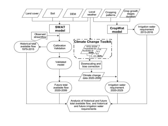
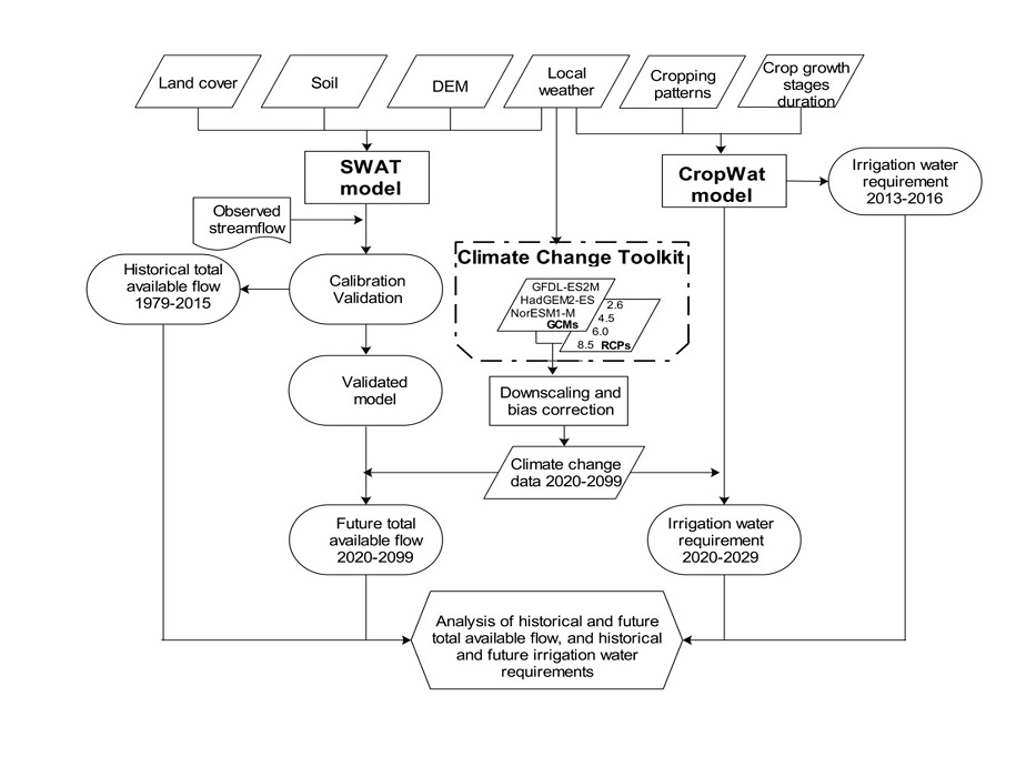
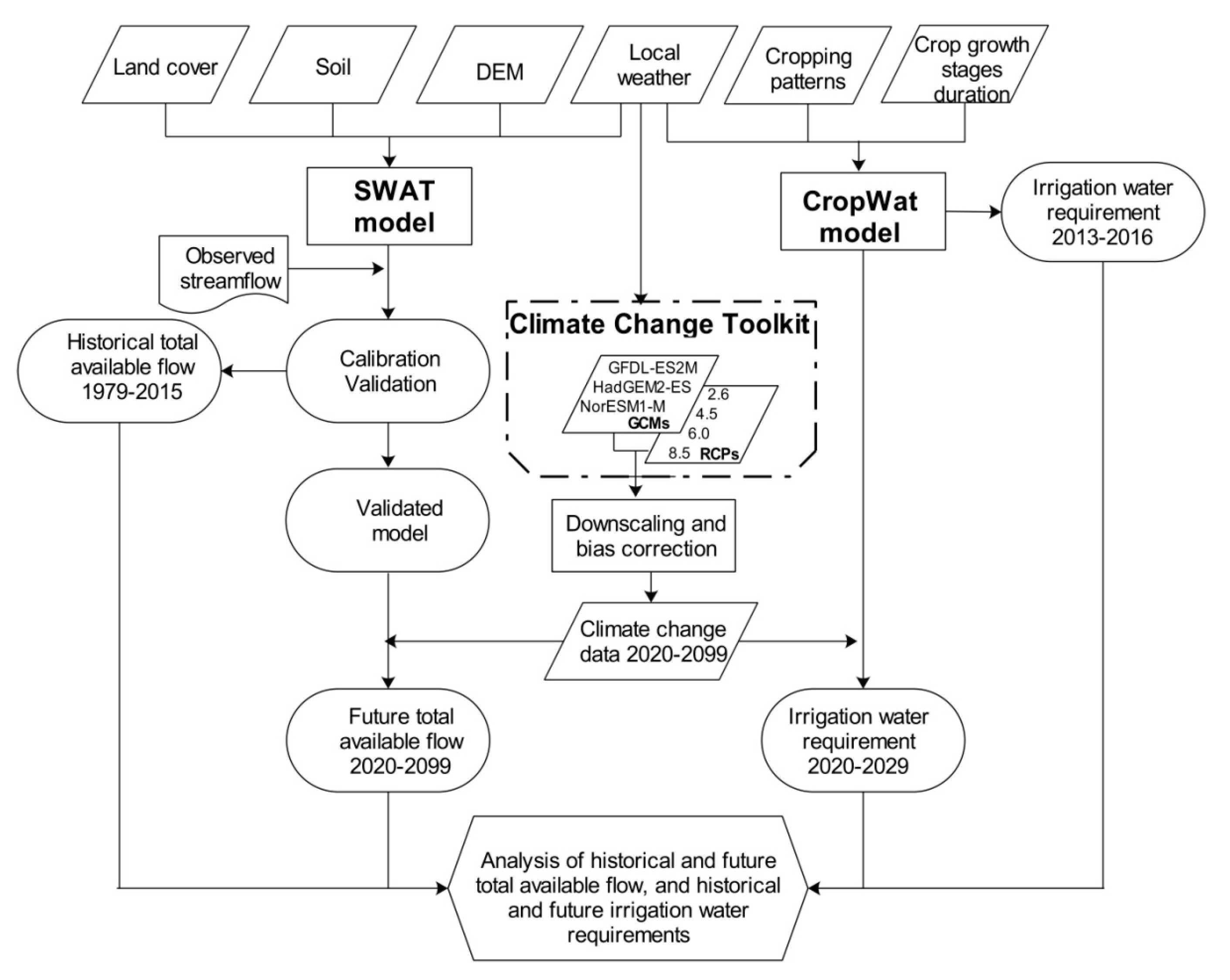
To estimate future scenarios, GCMs data from three models (General Fluids Dynamics Laboratory Earth System Model, GFDL-ES2M, Hadley-Centre Global Environment Model version 2, HadGEM2- ES, and Norwegian Climate Centers Earth System Model, NorESM1-M) was analyzed using the Climate Change Toolkit, CCT. CCT is a program developed by the Water Weather and Energy Ecosystem institute, Zurich, Switzerland, that handles climate change analysis tasks in one package. The program consists of six main modules: Data Extraction, Global Climate Data Management, Bias Correction and Statistical Downscaling, Spatial Interpolation and Critical Consecutive Day Analyzer. CCT is linked to an archive of historical global daily datasets (from the Climate Research Unit East Anglia [36]) and GCM models data from four carbon scenarios [37]. The output of CCT includes future climate variables (precipitation, minimum temperature and maximum temperature) which can be used to conduct future scenario analyses. The downscaled climate data from GCMs (with four RCPs each) was then used in both SWAT and CropWat models for future simulations). The results provide insights into water resource availability variations that can be used by MIS management in making informed future adaptation decisions. The methodological approach overview is shown in Figure 1.
2.2. Study Area
The climatic conditions around MIS are characterized by tropical weather dominated by monsoons. There are two rainy seasons: the short rain season (from October to November) and the long rain season (from April to May). The mean annual rainfall amount is about 930 mm. The temperature ranges between 14 °C and 31 °C. Relative humidity ranges from 55 to 70% in a day.
MIS receives irrigation water from the River Thiba and the River Nyamindi. The River Thiba sub basin, located in the Upper Tana catchment, receives only a small portion of the rainfall (about 4%) but contributes to nearly half of the sediment in the Masinga reservoir, which is located further downstream. This is because the River Thiba sub basin has a large number of small holder agricultures sites with longer periods of exposed soil as well as a relatively large area of rangelands [38]. MIS faces water shortages and as an adaptation strategy, the farmers are organized into three groups, which transplant rice at different times of the year in order to receive irrigation water during peak water demand times such as during transplanting. An adverse impact in rice production would affect a significant number of farmers, as this scheme produces about 80% of the local rice; the ripple effect would spread across the larger agricultural sector and the economy. The scheme is divided into two main irrigation systems: the Thiba system, which receives water from the River Thiba; and the Tebere system which receives water from the River Nyamindi. The two systems are subdivided into seven major irrigation blocks, namely the Mwea, Thiba, Wamumu, Karaba, and Curukia/Mutithi (for Thiba system) Tebere, and the Ndekia (for the Tebere system) as shown in Table 1.
Downstream past the scheme, the River Nyamindi flows into the River Thiba, which later flows into the larger River Tana, which is the largest river in Kenya. The catchment area for the River Tana covers approximately 17% of the country [39]. The Mwea Irrigation Scheme is divided into about 60 units, each with an average area of about 100 ha [40]. The irrigation block layout is shown in Figure 2.
2.3. Irrigation Block Water Requirement
The irrigation requirements from 2013–2016 were calculated using CropWat. The CropWat program consists of five data inputs (Climate, Rain, Crop, Soil and Cropping Pattern) and three calculation modules (Crop Water Requirement, Schedules and Scheme). The climate input is used to estimate the reference evapotranspiration, the rain input is used to estimate the effective rainfall, the crop input is used to estimate the actual crop evapotranspiration, and the soil input is used to estimate the soil moisture deficit. The length of the growth stages for the crops considered in this study were estimated based on Equation (1):
where GDD is Growing Degree Days, Tmax is the maximum temperature (°C), Tmin is the minimum temperature (°C), and Tbase is the base temperature for the crop (°C). The GDD was estimated using the daily maximum and minimum temperatures for the recorded temperature data (2013–2016) and the simulated future data. The growth stage duration was estimated from the growing degree days and accumulated heat values at the end of each stage (Equation (2)).
where GSD is Growth Stage Duration (days), Tacc is the accumulated heat value at the end of the stage (°C) and GDDc is the GDD for the corresponding period (°C). The reference crop base temperatures and accumulated heat stages at the end of the initial, development, mid-season and late season stages were obtained from the Food and Agriculture Organization database [41]. The method of growing degree days can be used to estimate the growth stage days for various crops [42,43].
GDD = [(Tmax + Tmin)/2] − Tbase
GSD = Tacc/GDDc
These inputs are used to estimate the crop water requirements. The scheme water requirements (in liters per second per hectare) are calculated after entering the specific planting dates, and the percentage areas of each crop. The irrigation water requirement for each block is estimated by multiplying the scheme water requirements and the irrigation area.
Due to the limited water resources, the farmers in the scheme are organized into three groups. An example of the existing cropping pattern is shown in Table 2.
Land preparation, e.g., rotavation, starts from the month of April, followed by the transplanting and growing period of the main crop which is harvested in early December. The ratoon rice crop then follows after the main crop and is harvested in March (ratoon rice crop is the rice crop that comes after harvesting and regenerates new panicle bearing tillers. It can be used to increase productivity where cropping intensity is limited by inadequate irrigation [44]). Future irrigation water requirement was estimated based on a new proposed cropping pattern. The proposed pattern seeks to diversify the crop production at MIS with long rain upland crops (mainly maize and vegetables) introduced between the months of February to June and short rain upland crops (mainly tomatoes and beans). A comparison of the existing and proposed cropping patterns is shown in Table 2.
To estimate irrigation water requirements for the 2013–2016 cropping seasons, climatic data (monthly means of precipitation, minimum temperature, maximum temperature and relative humidity) obtained from the Mwea Irrigation Agricultural Development (MIAD) weather station were input into CropWat. The local climatic data from the MIAD station was supplemented with other climatic data from the Climwat database (i.e., sunshine duration and wind speed from the Mwea Weather station number 21). Soil data (maximum infiltration rate, maximum rooting depths) for the predominant black cotton soils at MIS and rice crop data (crop coefficient Kc, rooting depth) were obtained from the CropWat database. The planting dates input into CropWat were the actual dates obtained from the MIS offices used for 2013–2016. A summary of the cropping patterns for rice obtained from the MIS offices is shown (Table 3).
To estimate the future irrigation water requirements, downloaded and downscaled climatic data (precipitation, minimum temperature and maximum temperature) from GCMs was input into CropWat. The soil data and rice crop data were also obtained from the CropWat database. The planting dates used for the future irrigation water requirements were 1st July for the main rice crop, 1st November for the ratoon rice, 1st October for the short rain upland crops and 1st March for the long rain upland crops. The proposed upland crops are tomatoes, maize, French bean, soy bean, green grams and vegetables. A summary of the irrigation areas for the proposed new cropping pattern is shown in Table 4.
2.4. Soil Water Assessment Tool (SWAT) Input
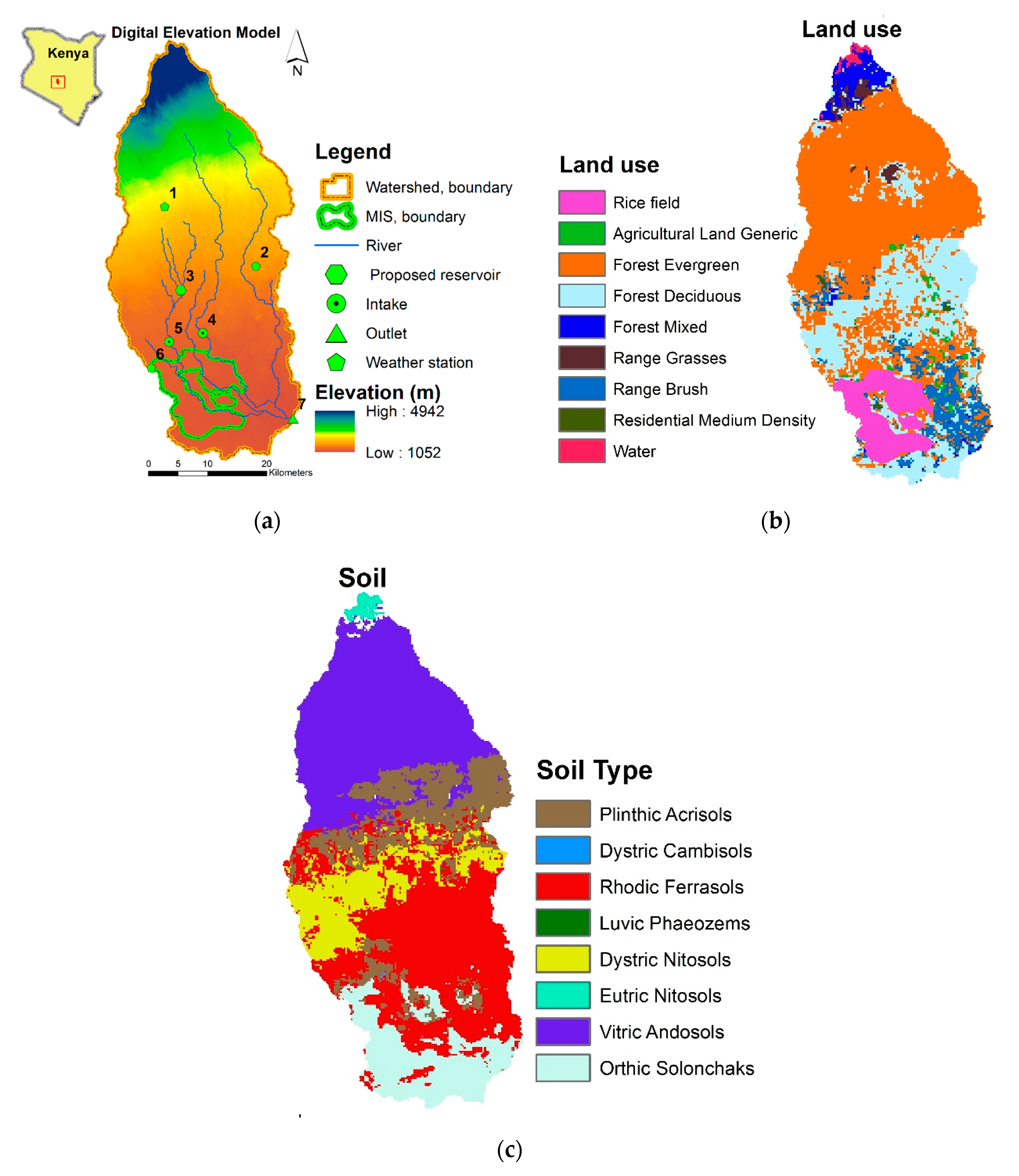
The SWAT model inputs were: Digital Elevation Model (DEM), soil map, land use map, and weather data. The SWAT 2012 ArcGIS interface [45] was used to discretize the River Thiba’s watershed, which was delineated from a 30 m Digital Elevation Model [46]. For the delineated watershed, the soil types and the land use of the study area were extracted from global databases of the Food and Agriculture Organization (FAO) [47] and Globcover [48] respectively, due to limited data availability in the study area. River discharge data and daily weather data were collected from the Kenya Water Resources Management Authority and the Kenya Meteorological Department, respectively. The local weather stations, Castle Forest, the Mwea Irrigation Agricultural Development Centre (MIAD) and Embu, are shown in Figure 3a as numbers 1, 2 and 6, respectively. The weir intakes on the River Nyamindi and the River Thiba are shown in Figure 3a as numbers 4 and 5, respectively. The proposed Thiba Dam location is shown as number 7. Due to data gaps and limited discharge measurements at the weir intakes, the River Gauging Station (RGS) 4DD02 (shown as number 7 in Figure 3a) was selected as the watershed outlet. The study area measures 1545 km2. The Digital Elevation Model, land use and soil maps are as shown in Figure 3. The delineation of the catchment study areas was done automatically in SWAT and stream networks were generated based on topography, flow direction and flow accumulation, discretizing 20 sub basins. The soil and land use maps were imported into SWAT and overlaid onto the DEM and the catchment was further subdivided into 351 spatial units known as Hydrologic Response Units (HRUs). Climate data was then imported into SWAT and once all the relevant input had been entered, the model was run.
The observed climate data from three weather stations; the watershed outlet point (at River RGS 4DD02) and intakes are as shown in Table 5.
SWAT simulation was done from 1979 to 2015 using observed historical data, with a two year warm-up period. The model was calibrated and validated for the periods 1981–1986 and 1987–1991, respectively using SWAT calibration and uncertainty programing [49]. After running the model, the simulated stream flow was evaluated using the Nash–Sutcliffe Efficiency (NSE) and percent bias (PBIAS) [50]. NSE is a normalized statistic that describes the relative magnitude of the residual variance as compared to the observed variance and demonstrates how well the plot of observed versus simulated fits the 1:1 line. PBIAS measures the average tendency of the simulated data to be larger or smaller than the observed counterparts [51]. After the simulation, determination of the rate of change in model output with respect to changes in input/parameters (sensitivity analysis) was done using the Sequential Uncertainty Fitting (SUFI-2) algorithm [52,53].
The simulated discharge data for the two weir intakes located on the River Thiba and the River Nyamindi were extracted from the SWAT output database files and were used to calculate the total available flow, i.e., the amount of water that can be abstracted from the two rivers for use in irrigation at MIS. These two intake points were selected because they are the sources of irrigation water for MIS, hence they can give a good estimation of the irrigation water available. The Water Resources Management Authority, Kenya [54] management rules were used to calculate the total available flow based on Equation (3):
where TAF is the Total Available Flow (m3 s−1), Q80 and Q95 represent the flow duration exceedance percentiles, which is the flow that can be expected to be equaled or exceeded 80% and 95% of the time, respectively (m3 s−1). (Q95 × 0.3) is the base flow requirements for the downstream riparian uses set at 30% of the environmental flow and AWR is the Accumulated Water Rights (m3 s−1). The Accumulated Water Rights were obtained from the Water Resources Management Authority, Kenya.
TAF = Q80 − (Q95 × 0.3) − AWR
To evaluate the water availability, a method described by Smakhtin et al. [55] considering the surface water available for withdrawals while meeting environmental water requirements was applied as shown in Equation (4).
where WSI is the Water Stress Index, MAR is the Mean Annual Runoff and EWR is the Environmental Water Requirement. In this study, the withdrawals considered are the estimated irrigation water requirements, and the component of (MAR–EWR) is considered as the Total Available Flow. The categorization of the Water Stress Index values based on Equation (4) is shown in Table 6.
WSI = Withdrawals/(MAR − EWR)
2.5. Climate Change Toolkit
The Climate Change Toolkit (CCT) has six main modules: Data Download, data extraction, Global Climate Data Management (GCDM), Bias Correction using Statistical Downscaling (BCSD), Spatial Interpolation of Climate Data (SICD) and Critical Consecutive Day Analyzer (CCDA) [37]. Observed climate data (precipitation, minimum and maximum temperatures) were obtained from three local weather stations (The Mwea Irrigation and Development Centre, MIAD, Castle Forest and Embu stations), defined by latitude, longitude and elevation were added to the CCT database.
Three sets of General Circulation Models, GCMs; GFDL-ESM2M (GCM 1) [56], HadGEM2-ES (GCM 2) [57]; and NorESM1-M (GCM 3) [58]) from the Inter-Sectoral Impact Model Inter-Comparison Project (ISI-MP) [59] (with four Representative Concentration Pathways, RCPs each i.e. RCP 2.6, 4.5, 6.0, 8.5) at 0.5° spatial resolution were used to obtain future climatic data. The Data Download module in CCT was used to download future climate data from the three GCMs (coordinates range from latitude −1° to 0°, and longitude 37 to 38°) from the Water Weather Energy Ecosystem website (www.2w2e.com). The GCM models, scenarios and periods downloaded are shown in Table 7.
The Data Extraction module was used to extract the climate data from the aforementioned coordinate range then regionalized to the coordinates of the observed data. The GCDM module was used to calculate the monthly averages, annual averages, long-term averages and anomalies of the weather stations. The BCSD module was used for downscaling by bias correcting the GCM future data using the observed climate data in the CCT database. Downscaling assigns the GCM data to the nearest observed user data. The SCID module was used to obtain finer resolution climate data. The Critical Consecutive Days Analyzer (CCDA) module was used to rewrite the data (from a bias-corrected and interpolation database), to separate the maximum and minimum temperature into different files and to specify coordinates and new names for each station’s data. The output of CCT was future precipitation and minimum and maximum temperatures data that were input into SWAT for future evaluation of irrigation water resources. The output from GCM station 435179 was used in estimating future irrigation water requirements as it is located within the MIS scheme. Table 8 shows the locations and elevations of the downscaled and bias-corrected GCM stations.
The weather stations data in Table 8 were input in SWAT and CropWat and were used to simulate the future total available flow (at the River Thiba and the River Nyamindi weir intakes) and future irrigation water requirements, respectively. The frequency analysis of the data was estimated using probability of exceedance. For irrigation systems, rainfall depths with probabilities of exceedance of 75–80% are often selected [60]. A period of 30 years and over is normally thought to be very satisfactory for climate data analysis [61]. For this study, 80% probability of exceedance was applied for two periods (2020–2060 and 2061–2099).
3. Results
3.1. Water Demand Analysis
The 2013–2016 cropping season water requirements were calculated based on Table 3. The irrigation water requirement was calculated for each group and was summed-up to show the total irrigation water requirement of each of the cropping season analyzed.
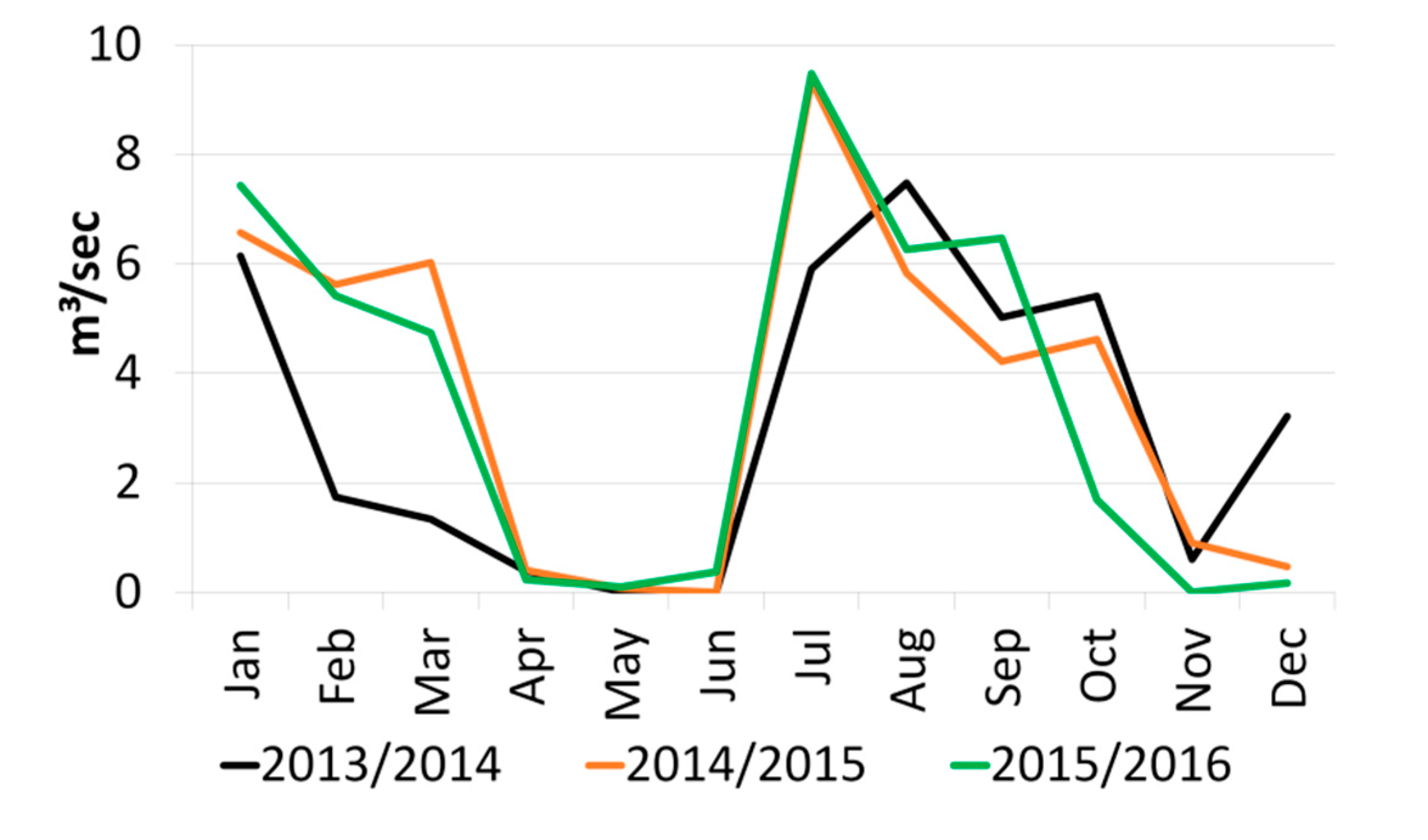
Across the three seasons analyzed, the peak water demand was the July 2015/2016 season (9.4 m3 s−1). With the onset of the short rains in October/November, the irrigation water requirement decreased. There was a trend of the highest peak water demand for the scheme in the months of July/August, and then a subsequent decrease was observed in all the seasons analyzed, as shown in Figure 4.
3.2. Estimation of Total Available Flow at the River Thiba and the River Nyamindi
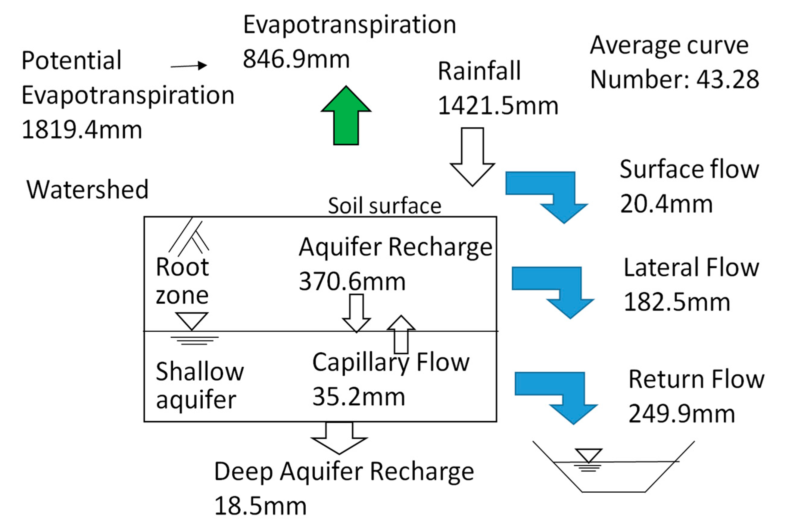
Calibration of the SWAT model was done to allow for a better physical representation of the functioning of the modeled study area. NSE was selected as an objective function for the model calibration for this study. The initial range of the calibrated parameters was set to default values provided by the SWAT-Cup program. Calibration of the model was done by optimizing the parameter range until the objective function of the output variable achieved a satisfactory value. The most sensitive parameters for this simulation were curve number (R__CN2.mgt), ground water delay time (V__GW_DELAY.gw), threshold water depth in the shallow aquifer (V__GWQMN.gw), available water capacity (V__SOL_AWC.sol) and base flow factor (V__ALPHA_BF.gw). After several iterations, the satisfactory NSE and PBIAS calibration objective function values were obtained (shown in Table 9) with the optimized parameters (shown in Table 10). The modeled hydrological characteristics of the watershed are shown in Figure 5 (model calibration and validation) and Figure 6 (hydrological summary of the watershed simulation). According to the simulated hydrology, only a small fraction (1.43%) of precipitation became surface runoff, while the majority (60%) of rainfall in the watershed was evaporated and transpired. The percolation and lateral flow accounted for 26% and 12% of the precipitation, respectively. Therefore, the simulated hydrology components showed that the watershed was characterized by dominant groundwater. This could be as a result of the high percentage of forested areas (81%) in the land use, particularly in the central to northern parts of the watershed (part of the watershed lies within Mount Kenya forest). The forested areas can influence the surface runoff and increase the ratio of groundwater recharge [62]. The performance of the model calibration and validation, parameters and hydrology summary are shown in Figure 5 and Figure 6 and in Table 9 and Table 10.
Generally, performance ratings of NSE values between 0.50 < NSE ≤ 0.65 can be described as satisfactory. NSE values of 0.75 < NSE ≤ 1.00 can be described as very good. For PBIAS, values ±15 ≤ PBIAS < ±30 can be described as good, and values PBIAS < ±15 can be described as very good [50]. The SWAT model simulation of this study can be described as satisfactory, though future simulations could be improved by making use of more local data inputs (such as soils, land use, DEM). Figure 6 shows the hydrological summary of the watershed simulation
3.3. Comparison of Total Available Flow and Water Demand (2013–2016)
The current water resources available in the River Thiba and the River Nyamindi were highest in the month of May (5.0 m3 s−1 and 4.5 m3 s−1, respectively) and lowest in the month of March (1.6 m3 s−1 and 0.8 m3 s−1, respectively) as shown in Figure 7. The highest irrigation water deficits were observed in the months of July (up to 4.9 m3 s−1) and August (up to 4.1 m3 s−1). Surplus irrigation water was observed to be available in the months of November to December (ranging from 2.6 m3 s−1 to 6.0 m3 s−1) after the short rain season.
3.4. Climate Change Modeling
SWAT was run again (after the calibration and validation) using the downloaded, downscaled and bias-corrected future climate data from the three GCMs (four RCPs each) to analyze future total available flow at the two weir intakes on the River Thiba and the River Nyamindi. The future irrigation water requirement was also estimated using the future climate data from the three GCMs (four RCPs each). Figure 8, Figure 9, Figure 10 and Figure 11 show the future water total available flow and irrigation water requirement comparisons under RCPs 2.6, 4.5, 6.0 and 8.5, respectively for two time periods, i.e., 2020–2060 and 2061–2099.
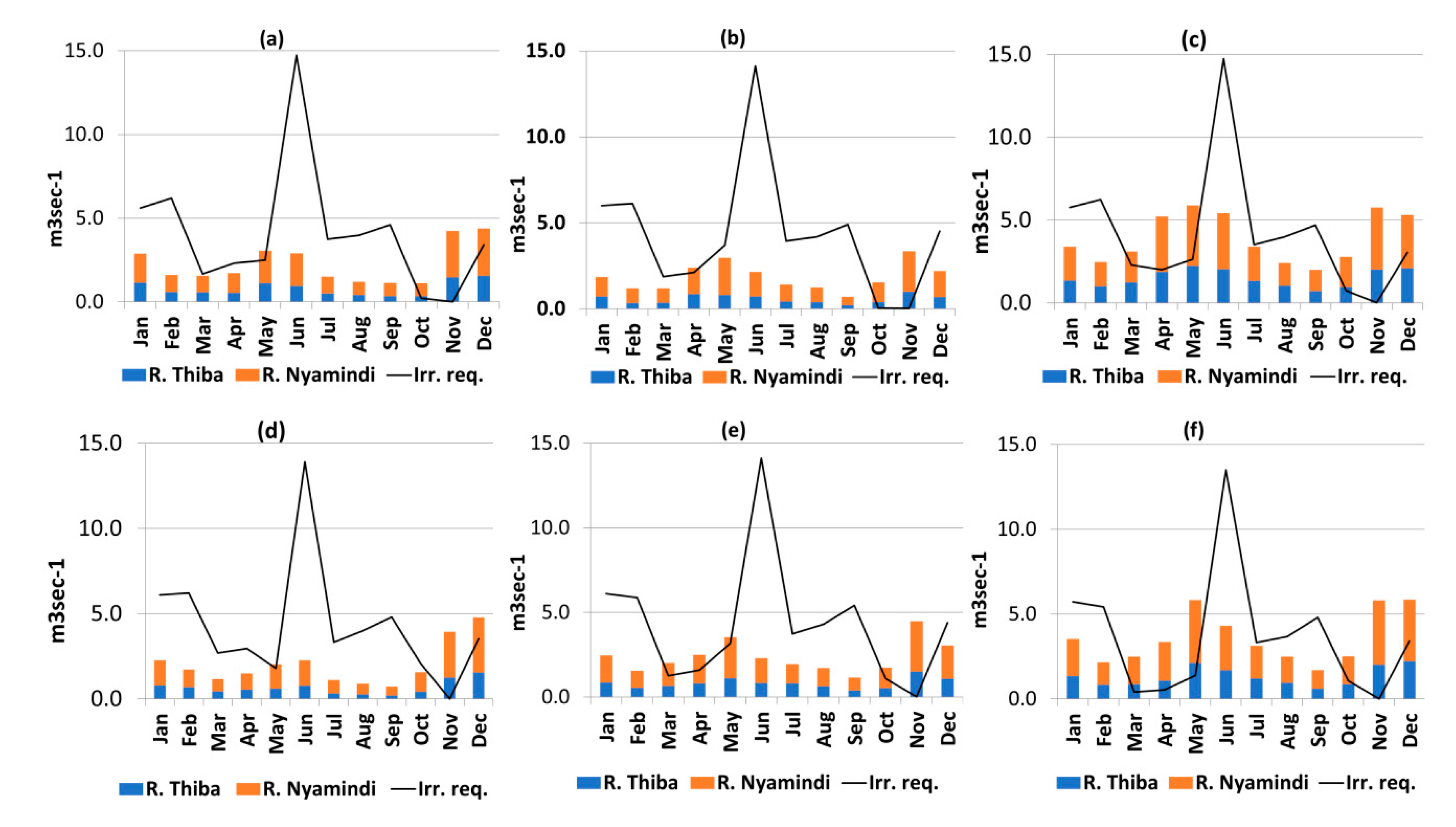
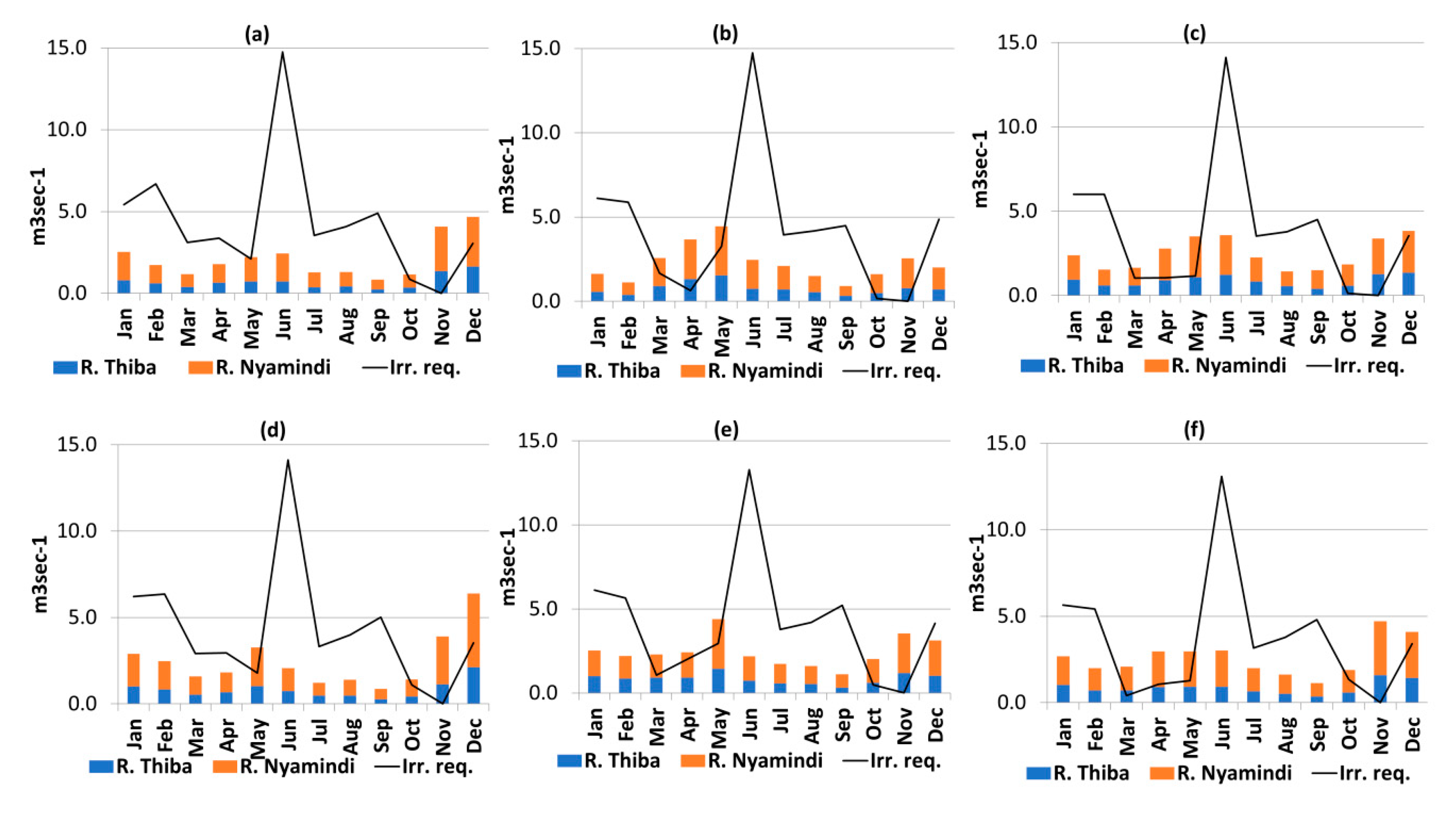
Under RCP 2.6, the highest total available flow was observed in the months of May, November and December; and the least in the month of February for both the 2020–2060 and the 2061–2099 periods (Figure 8a,b,d,e). The highest irrigation water requirements were observed to be the highest in the months of June (14.7 m3 s−1 under GCM 1 and 2 in 2020–2060) and the least in the month of November (0.2 m3 s−1 under GCM 1) as shown in Figure 8c,e.
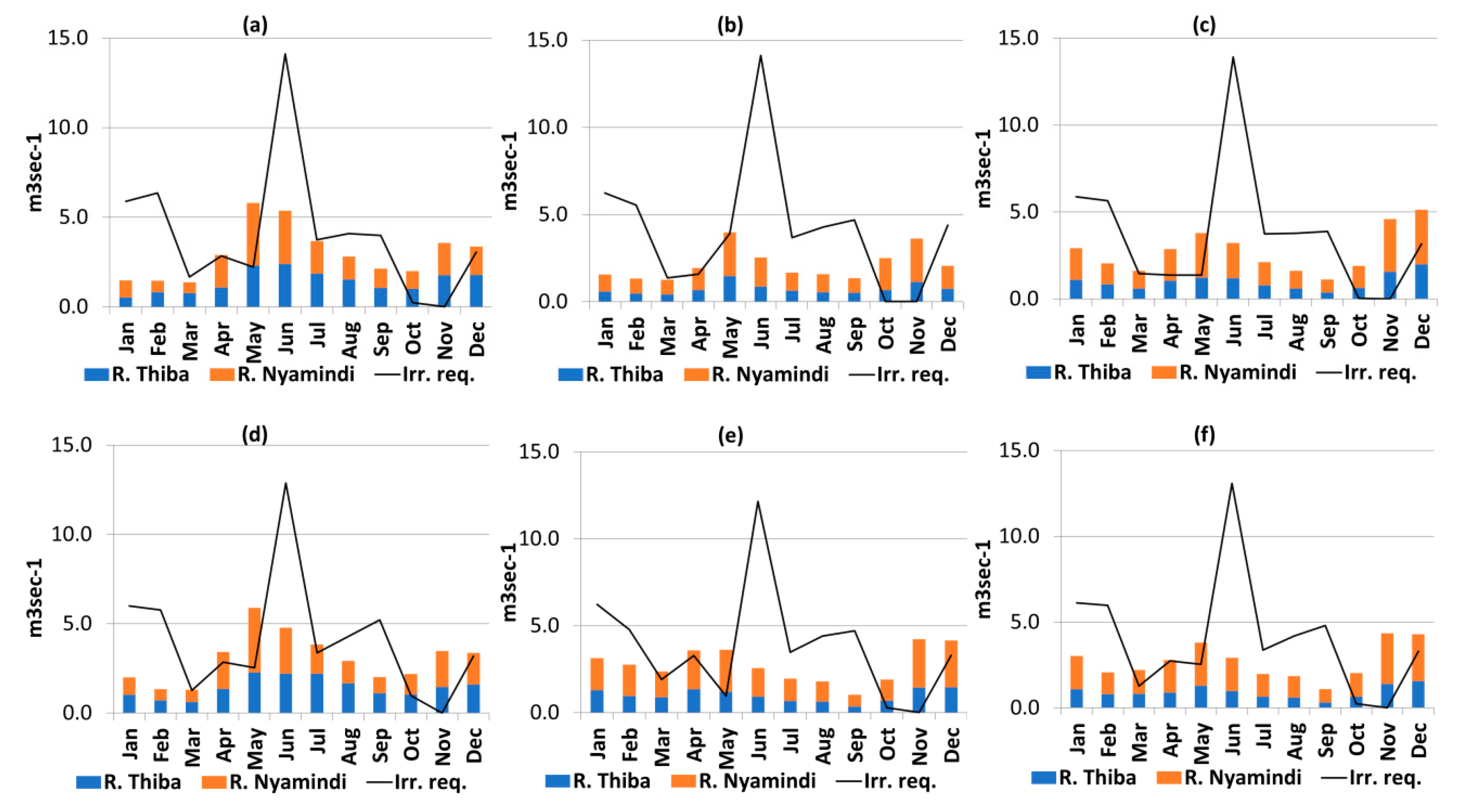
RCP 4.5 showed the highest total available flow in the months of May, November and December (Figure 9a,b,d,e). The highest irrigation water requirements were observed to be the highest in the months of June (14.1 m3 s−1 under GCM 3 in 2020–2060) and the lowest irrigation water requirements in the month of November (0.1 m3 s−1 under GCM 3 in 2020–2060 period and 0.2 m3 s−1 under GCM 2 for 2020–2060 period). Total available flow was observed to be greater than irrigation water requirements in the month of November.
RCP 6.0 shows the highest total available flow in the months of May, November and December, and the lowest in the month of February (Figure 10a,b,d,e). The highest irrigation water requirements were observed in the month of June (14.5 m3 s−1 under GCM 2, 2020–2060 period) and the least in the month of October (0.3 m³/s under GCM 3, 2060–2099 period) as shown in Figure 10c,f.
RCP 8.5 shows the highest total available flow in the months of May, November and December; and the lowest in the month of February (Figure 11a,b,d,e). The highest irrigation water requirements were observed to be the highest in the month of June (14.1 m3 s−1 under GCM 2, 2020–2060 period) and the least in the month of October (0.2 m³/s under GCM 3, 2061–2099 period) as shown in Figure 11c,f.
MIS plans to develop a dam on the River Thiba to address the current water deficits experienced at the scheme. The dam is planned to be an irrigation-only dam to provide supplemental irrigation water. A comparison of the future total available flow (summation of the River Thiba and the River Nyamindi) and irrigation water requirements was done to estimate the future Water Stress Index (WSI) at MIS for the three GCMs and two time periods (i.e., 2020–2060 and 2061–2099) is shown in Table 11, Table 12, Table 13 and Table 14 for RCP 2.6, 4.5, 6.0 and 8.5, respectively.
RCP 2.6 showed the highest irrigation deficits in the month of June and February, with subsequent high WSI (highest observed as 6.58 under GCM 2 in the 2020–2060 period). Irrigation deficits were also observed in the months of July to October and January. A surplus of irrigation water was observed mainly in the month of November (The zero values denote a surplus in irrigation water). RCP 4.5 showed the highest WSI in the months of June, September and February (the highest was observed as 6.82 in the 2061–2099 period under GCM 1).
RCP 6.0 showed the highest WSI in the months of June, September and February (highest observed as 5.98 under GCM 1 in 2020–2060). A surplus of irrigation water was observed in the month of November, and moderate exploitation of water resources in the month of April and May. RCP 8.5 had the highest WSI observed in the months of June, January and February (highest observed as 5.54 in the 2020–2060 period under GCM 2). Surplus irrigation water was observed in the month of November.
Across all the RCPs and time periods, the months of January–February and June–September have a strong trend of irrigation water being insufficient to meet the water demand, indicating a strong over-exploitation of the water resources in the study area. The months of March–May show that some variations have a strong trend towards displaying water surplus. Being the largest irrigation scheme in Kenya, the results of this MIS case study results in support for the country-based classification of Kenya as a country where, in the future, surface water resources could likely be unable to meet the irrigation water demand according to an index for assessing the potential for future agriculture in Sub Saharan Africa developed by Nizar et al. [31]
4. Discussion
4.1. Water Shortage Timing
The peak irrigation water requirements (in m3 s−1) were estimated to be between the months of July and August, which mainly fall within the land preparation period. Most of the farmers would prefer to transplant at the beginning of the short rain season and harvest between November and December when there is a high demand for rice due to the long Christmas holidays. However, they are required to follow the cropping calendar provided. Climatic conditions make planting in the long rain season (April–May) less favorable due to higher susceptibility to rice blast disease, which has been reported to cause about 60–70% of the yield losses [64]. Since most of the farms are operated using family labor and they primarily rely on rice farming as their main source of income [65], MIS management will have to ensure adequate water availability for the main rice crop to ensure farmers can harvest and sustain their livelihoods. The water shortage may be exacerbated by withdrawal of water from the main canals for other illegal uses, as observed during our field studies in 2018 and 2019. The withdrawals observed included use of water for domestic use at home and for running small car wash businesses along major roads within the scheme. Such withdrawals are difficult to quantify and were not considered in this study.
Previous studies indicated that horticultural farms located upstream of MIS abstract water from the River Thiba and the River Nyamindi, thus contributing to a reduction in the water available for the scheme. A survey conducted in 1997 indicated that about 10% of the abstractions were legal [40]. The MIS management can put forward proposals to the relevant government authorities for more stringent policies that could be used to monitor and control water abstraction in rivers and to protect the MIS farmers against water shortages. In addition, local community sensitization on the importance of irrigation water could also play a role in community policing and monitoring of illegal water abstractions. The extent of water shortage for irrigation can also be used by the relevant government authorities (such as the Water Resources Authority, Kenya) in guiding/controlling the issuance of permits for abstraction of water for other purposes. This could play an important role in increasing water availability for irrigation.
4.2. Impact of Climate Change
Across the two periods analyzed for all GCMs, the highest future water deficits were estimated to be in the months of June, representing a shift from the month of July as observed in 2013–2016. Under the proposed cropping program (that is supposed to used after the dam construction), the main rice crop will heavily rely on irrigation water from the dam throughout its growth stages from transplanting to harvesting. This is because the main rice crop falls between the periods of July to October. This period was observed to have a strong predominance of water deficits across all GCM simulations. Water stored in the dam after the long rains (April/May) should be carefully released for the main rice crop mainly during land preparation and transplanting in the months of June and July. A decrease in the amount of long rains would have an impact on the main rice crop. Future farming practices should take into consideration the water availability in the high water deficit months and explore the options of reducing the water deficits such as practicing more efficient rice irrigation methods.
There have been initiatives to introduce water-saving irrigation practices at MIS over the years, most notably in the Rice-Based and Market-Oriented Agriculture Promotion Project (RiceMAPP) in demonstration farms [66]. Such initiatives take into consideration water-saving practices as a way of reducing water use, and the larger aspect of climate change would require adequate sensitization and training of farmers in order for them to be successfully implemented. A previous study on the socio-economic status of farmers at MIS conducted in 2013 indicated that about 43% of small-scale farmers at MIS had completed a high school education. Increased government efforts in raising the education level of farmers could contribute to better sensitization, learning and training of farmers on new and better water-saving technologies, promote a strong participatory approach, and contribute to combating the impacts of climate change. Such water-saving initiatives could be taken into strong consideration and could contribute to a reduction of the high peak water demands compared to the current conventional flooding irrigation methods.
4.3. Adaptation of Cropping Pattern
Under the proposed cropping pattern, the total land area under irrigation is 17,900 ha for the long and short rains upland crops; and short rain rice and ratoon rice. In the existing cropping pattern, the land areas under irrigation for the 2013/2014, 2014/2015 and 2015/2016 seasons were 7890 ha, 8095 ha and 8903 ha respectively. With the expected increase in land area under irrigation and the introduction of new upland crops, farmers will have to adapt to water management, particularly in the months with high water deficits.
The proposed short rain upland crops fall within the months of October and January. The months of November and December were evaluated to have surplus irrigation water in the future period. With careful management of dam irrigation water, MIS management can explore the opportunity for utilizing the surplus water. Cropping intensities for the short rain upland crops could be increased to make use of the surplus water, hence improving production in the future.
The month of February, which falls at the beginning of the long rain upland crops in the proposed cropping pattern, was observed to have the second highest irrigation water deficit. Farmers will predominantly rely on irrigation water during the planting stage. MIS management should plan for careful management of the dam irrigation water and ensure that irrigation water is available during this important time for the long rain upland crops. The mid-season stage for the upland crops falls during the long rain season (April/May) when surplus irrigation water was observed to be available. The methodological approach presented in this study could be adopted for guiding the development of cropping patterns within the East African region to tap into the irrigation potential. Identification of projected water shortages and surplus months can play an important role for farmers in increasing their efficiency and productivity.
5. Conclusions
This study’s objective was achieved through applying a SWAT model to estimate the current and future water resources (as total available flow) and CropWat to estimate irrigation water requirements. Downloaded, spatially interpolated, downscaled and bias-corrected future climate data from a Climate Change Toolkit were input into SWAT and CropWat to simulate future scenarios. The future climate data was also input into CropWat to analyze future irrigation water requirements. The results show that the highest irrigation water deficits will be experienced in the month of June. The months of July–October and January–February are also expected to have deficits. Surplus irrigation water is expected to be observed in the months of November and December in the future. The results could be useful to MIS in estimation of water availability, addressing climate change impacts through a participatory approach with farmers and the government, developing cropping patterns and an overall improvement of planning and water management at MIS. This study aspires to contribute to water availability research by presenting a methodological framework for current and future water resource availability for irrigation planning and management in regions where data availability may be inadequate but there exists a future irrigation development potential.
A major limitation in this study was the lack of data for calibrating the CropWat estimations. With due attention to this limitation, findings of this study can be used for the improvement of irrigation water resource planning and management. In the future, after the implementation of a dam on the River Thiba, data monitoring in dam release, stream flow, sediment in the river (and in the reservoir) and canal flows should be conducted for future modeling of the Thiba dam and MIS. This would allow for analysis such as future dam irrigation water supply and sediment inflow into the reservoir to estimate future maintenance/dredging costs. Data monitoring on irrigation water quality, irrigation conveyance and drainage canals should be conducted to monitor any water losses. Also, strong considerations should be made for conducting soil tests at MIS watershed area. The soil data could be very useful in SWAT simulations as well as in CropWat data input in order to reduce the bias in the estimations of total available flow and irrigation water requirements.
Author Contributions
G.A. (Conceptualization, Investigation, Methodology, Software, Validation, Formal analysis, Writing—original draft preparation), L.H.T. (Methodology, Software, Validation, Formal Analysis), T.K. (Conceptualization, Resources, Supervision, Writing—review and editing). All authors have read and agreed to the published version of the manuscript.
Funding
This research received no external funding.
Acknowledgments
The author gratefully acknowledges the technical staff at the Mwea Irrigation Scheme, resident engineers at the Thiba Dam project, Water Resources Management Authority (Kenya) for their all rounded support and cooperation in availing the necessary data and support during the fieldwork studies. Our deepest gratitude is also extended to the Tokyo University of Agriculture and Technology (Japan) for their financial support during the course of this study. The authors are grateful to the anonymous reviewers for their constructive suggestions.
Conflicts of Interest
The authors declare no conflict of interest.
References
- Fairhurst, T.; Dobermann, A. Rice in the global food supply. Better Crops Int. 2002, 16, 1–6. [Google Scholar]
- Dobermann, A.; Fairhurst, T. International Rice Research Institute. In Rice: Nutrient Disorders & Nutrient Management; Potash & Phosphate Institute, East & Southeast Asia Programs: Singapore; IRRI: Makati City, Philippines, 2000; ISBN 978-981-04-2742-9. [Google Scholar]
- Ministry of Planning, Kenya. Kenya Vision 2030 | Kenya Vision 2030. 2008. Available online: http://vision2030.go.ke/ (accessed on 10 October 2019).
- Hunink, J.E.; Niadas, I.A.; Antonaropoulos, P.; Droogers, P.; de Vente, J. Targeting of intervention areas to reduce reservoir sedimentation in the Tana catchment (Kenya) using SWAT. Hydrol. Sci. J. 2013, 58, 600–614. [Google Scholar] [CrossRef] [Green Version]
- GIBB Africa Limited. Mwea Irrigation Scheme Water Management Improvement Project; GIBB Africa Limited: Nairobi, Kenya, 2010; p. 13. [Google Scholar]
- IPCC. AR4 Climate Change 2007: The Physical Science Basis—IPCC; IPCC: Geneva, Switzerland, 2007. [Google Scholar]
- IPCC. Working Group I Contribution to the Fifth Assessment Report of the Intergovernmental Panel on Climate Change; Stocker, T.F., Qin, D., Plattner, G.-K., Tignor, M.M.B., Allen, S.K., Boschung, J., Nauels, A., Xia, Y., Bex, V., Midgley, P.M., Eds.; Cambridge University Press: Cambridge, UK, 2013; p. 14. [Google Scholar]
- Dixon, K.W.; Lanzante, J.R.; Nath, M.J.; Hayhoe, K.; Stoner, A.; Radhakrishnan, A.; Balaji, V.; Gaitán, C.F. Evaluating the stationarity assumption in statistically downscaled climate projections: Is past performance an indicator of future results? Clim. Chang. 2016, 135, 395–408. [Google Scholar] [CrossRef] [Green Version]
- van Vuuren, D.P.; Edmonds, J.; Kainuma, M.; Riahi, K.; Thomson, A.; Hibbard, K.; Hurtt, G.C.; Kram, T.; Krey, V.; Lamarque, J.-F.; et al. The representative concentration pathways: An overview. Clim. Chang. 2011, 109, 5–31. [Google Scholar] [CrossRef]
- Darwin, R.; Tsigas, M.; Lewandrowski, J.; Raneses, A. World Agriculture and Climate Change; Agricultural Economic Report No. 703; United States Department of Agriculture Economic Research Service: Washington, DC, USA, 1995; p. 98.
- Basheer, A.; Lü, H.; Omer, A.; Ali, A.; Abdelgader, A. Impacts of climate change under CMIP5 RCP scenarios on the streamflow in the Dinder River and ecosystem habitats in Dinder National Park, Sudan. Hydrol. Earth Syst. Sci. Discuss. 2015, 12, 10157–10195. [Google Scholar] [CrossRef]
- Näschen, K.; Diekkrüger, B.; Leemhuis, C.; Seregina, L.; van der Linden, R. Impact of climate change on water resources in the Kilombero catchment in Tanzania. Water 2019, 11, 859. [Google Scholar] [CrossRef] [Green Version]
- Roth, V.; Lemann, T.; Zeleke, G.; Subhatu, A.T.; Nigussie, T.K.; Hurni, H. Effects of climate change on water resources in the upper Blue Nile Basin of Ethiopia. Heliyon 2018, 4, e00771. [Google Scholar] [CrossRef] [Green Version]
- Nakawuka, P.; Langan, S.; Schmitter, P.; Barron, J. A review of trends, constraints and opportunities of smallholder irrigation in East Africa. Glob. Food Secur. 2018, 17, 196–212. [Google Scholar] [CrossRef]
- Neitch, S.L.; Arnold, J.G.; Kiniry, J.R.; Williams, J.R. Soil and Water Assessment Tool Theoretical Document (Version 2009); Blackland Research Center: Temple, TX, USA, 2009. [Google Scholar]
- Yesuf, H.M.; Melesse, A.M.; Zeleke, G.; Alamirew, T. Streamflow prediction uncertainty analysis and verification of SWAT model in a tropical watershed. Environ. Earth Sci. 2016, 75, 806. [Google Scholar] [CrossRef]
- Gassman, P.W.; Reyes, M.R.; Green, C.H.; Arnold, J.G. The soil and water assessment tool: Historical development, applications, and future research directions. Trans. ASABE 2007, 50, 1211–1250. [Google Scholar] [CrossRef] [Green Version]
- Githui, F.; Gitau, W.; Mutua, F.; Bauwens, W. Climate change impact on SWAT simulated streamflow in western Kenya. Int. J. Climatol. 2009, 29, 1823–1834. [Google Scholar] [CrossRef]
- Musau, J.; Sang, J.; Gathenya, J.; Luedeling, E. Hydrological responses to climate change in Mt. Elgon watersheds. J. Hydrol. Reg. Stud. 2015, 3, 233–246. [Google Scholar] [CrossRef] [Green Version]
- Anadranistakis, M.; Liakatas, A.; Kerkides, P.; Rizos, S.; Gavanosis, J.; Poulovassilis, A. Crop water requirement model tested for crops grown in Greece. Agric. Water Manag. 2000, 45, 297–316. [Google Scholar] [CrossRef]
- Mimi, Z.A.; Jamous, S.A. Climate change and agricultural water demand: Impacts and adaptations. Afr. J. Environ. Sci. Technol. 2010, 4. [Google Scholar] [CrossRef]
- Nazeer, M. Simulation of maize crop under irrigated and rainfed conditions with CROPWAT model. J. Agric. Biol. Sci. 2009, 4, 68–73. [Google Scholar]
- Kang, S.; Payne, W.; Evett, S.; Robinson, C.; Stewart, B. Simulation of winter wheat evapotranspiration in Texas and Henan using three models of differing complexity. Agric. Water Manag. 2009, 96, 167–178. [Google Scholar] [CrossRef]
- Aldaya, M.M. The Water Footprint Assessment Manual: Setting the Global Standard, 1st ed.; Routledge: Abingdon, UK, 2012; ISBN 978-1-84977-552-6. [Google Scholar]
- Núñez, M.; Pfister, S.; Antón, A.; Muñoz, P.; Hellweg, S.; Koehler, A.; Rieradevall, J. Assessing the environmental impact of water consumption by energy crops grown in Spain. J. Ind. Ecol. 2013, 17, 90–102. [Google Scholar] [CrossRef]
- Ridoutt, B.G.; Pfister, S. A revised approach to water footprinting to make transparent the impacts of consumption and production on global freshwater scarcity. Glob. Environ. Chang. 2010, 20, 113–120. [Google Scholar] [CrossRef]
- Xu, H.; Wu, M. Water Availability Indices–A Literature Review; Argonne National Laboratory: Lemont, IL, USA, 2017. [Google Scholar]
- Xu, H.; Wu, M. A first estimation of county-based green water availability and its implications for agriculture and bioenergy production in the United States. Water 2018, 10, 148. [Google Scholar] [CrossRef] [Green Version]
- Kummu, M.; Guillaume, J.H.A.; de Moel, H.; Eisner, S.; Flörke, M.; Porkka, M.; Siebert, S.; Veldkamp, T.I.E.; Ward, P.J. The world’s road to water scarcity: Shortage and stress in the 20th century and pathways towards sustainability. Sci. Rep. 2016, 6, 38495. [Google Scholar] [CrossRef] [Green Version]
- Moore, B.; Coleman, A.; Wigmosta, M.; Skaggs, R.; Venteris, E. A high spatiotemporal assessment of consumptive water use and water scarcity in the conterminous United States. Water Resour. Manag. 2015, 29. [Google Scholar] [CrossRef]
- Abou Zaki, N.; Torabi Haghighi, A.; Rossi, P.; Xenarios, S.; Kløve, B. An Index-based approach to assess the water availability for irrigated agriculture in Sub-Saharan Africa. Water 2018, 10, 896. [Google Scholar] [CrossRef] [Green Version]
- Uniyal, B.; Dietrich, J.; Vu, N.Q.; Jha, M.K.; Arumí, J.L. Simulation of regional irrigation requirement with SWAT in different agro-climatic zones driven by observed climate and two reanalysis datasets. Sci. Total Environ. 2019, 649, 846–865. [Google Scholar] [CrossRef] [PubMed]
- Maier, N.; Dietrich, J. Using SWAT for strategic planning of basin scale irrigation control policies: A case study from a humid region in Northern Germany. Water Resour. Manag. 2016, 30, 3285–3298. [Google Scholar] [CrossRef]
- Tibebe, M.; Melesse, A.; Zemadim, B. Runoff estimation and water demand analysis for Holetta river, Awash Subbasin, Ethiopia using SWAT and CropWat models. In Landscape Dynamics, Soils and Hydrological Processes in Varied Climates; Melesse, A.M., Abtew, W., Eds.; Springer Geography; Springer: Cham, Switzerland, 2015; pp. 113–140. ISBN 978-3-319-18787-7. [Google Scholar]
- Fu, Q.; Yang, L.; Li, H.; Li, T.; Liu, D.; Ji, Y.; Li, M.; Zhang, Y. Study on the optimization of dry land irrigation schedule in the downstream Songhua river basin based on the SWAT model. Water 2019, 11, 1147. [Google Scholar] [CrossRef] [Green Version]
- Harris, I.; Jones, P.D.; Osborn, T.J.; Lister, D.H. Updated high-resolution grids of monthly climatic observations—The CRU TS3.10 Dataset. Int. J. Climatol. 2014, 34, 623–642. [Google Scholar] [CrossRef] [Green Version]
- Ashraf Vaghefi, S.; Abbaspour, N.; Kamali, B.; Abbaspour, K.C. A toolkit for climate change analysis and pattern recognition for extreme weather conditions—Case study: California-Baja California Peninsula. Environ. Model. Softw. 2017, 96, 181–198. [Google Scholar] [CrossRef]
- Jacobs, J.H.; Angerer, J.; Vitale, J.; Srinivasan, R.; Kaitho, R. Mitigating economic damage in Kenya’s upper Tana River Basin: An application of arc-view SWAT. J. Spat. Hydrol. 2007, 7, 23–46. [Google Scholar]
- Pacini, N.; Harper, D.; Mavuti, K. Hydrological and ecological considerations in the management of a catchment controlled by a reservoir cascade: The Tana river, Kenya. In The Sustainable Management of Tropical Catchments; Harper, D., Brown, T., Eds.; John Wiley & Sons: Indianapolis, IN, USA, 1998; pp. 239–258. [Google Scholar]
- Mohammed, A.; Mizutani, M.; Tanaka, S.; Goto, A.; Matsui, H. Changes in water management practices in the Mwea irrigation scheme, Kenya from 1994 to 1998. Rural Environ. Eng. 2003, 44, 60–67. [Google Scholar]
- Studeto, P.; Theodore, H.; Fereres, E.; Raes, D. Crop Yield Response to Water; FAO Irrigation and Drainage Paper; Food and Agriculture Organization of the United Nations: Rome, Italy, 2012; Volume 66, ISBN 978-92-5-107274-5. [Google Scholar]
- Acharjee, T.K.; Ludwig, F.; van Halsema, G.; Hellegers, P.; Supit, I. Future changes in water requirements of Boro rice in the face of climate change in North-West Bangladesh. Agric. Water Manag. 2017, 194, 172–183. [Google Scholar] [CrossRef]
- Miller, P.; Lanier, W.; Brandt, S. Using Growing Degree Days to Predict Plant Stages; Montana State University Extension: Bozeman, MT, USA, 2018; p. 8. [Google Scholar]
- International Rice Research Institute. Rice Ratooning; International Rice Research Institute: Los Banos, Manila, Philippines, 1998; ISBN 971-10-4190-1. [Google Scholar]
- Winchell, M.; Srinivasan, R.; Di Luzio, M.; Arnold, J.G. ArcSWAT Interface for SWAT Users Guide. Available online: https://swat.tamu.edu/software/arcswat/ (accessed on 21 October 2019).
- USGS.gov. USGS.gov|Science for a Changing World. Available online: https://www.usgs.gov/ (accessed on 10 October 2019).
- Food and Agriculture Organization of the United Nations. FAO Digital Soil Map of the World (DSMW)|Land & Water|Food and Agriculture Organization of the United Nations|Land & Water|Food and Agriculture Organization of the United Nations. Available online: http://www.fao.org/land-water/land/land-governance/land-resources-planning-toolbox/category/details/en/c/1026564/ (accessed on 10 October 2019).
- ESA. ESA Data User Element. Available online: http://due.esrin.esa.int/page_globcover.php (accessed on 10 October 2019).
- Abbaspour, K.C. SWAT Calibration and Uncertainty Programs; EAWAG: Swiss Federal Insitute of Aquatic Science and Technology: Dübendorf, Switzerland, 2015; p. 100. [Google Scholar]
- Moriasi, D.N.; Arnold, J.G.; Bingner, R.L.; Van Liew, M.W.; Harmel, R.D.; Veith, T.L. Model evaluation guidelines for systematic quantification of accuracy in watershed simulations. ASABE 2007, 50, 885–900. [Google Scholar] [CrossRef]
- Kidane, W.; Bogale, G. Effect of land use land cover dynamics on hydrological response of watershed: Case study of Tekeze Dam watershed, Northern Ethiopia. ISWCR 2017, 5, 1–16. [Google Scholar] [CrossRef]
- Abbaspour, K.C.; Johnson, C.A.; van Genuchten, M.T. Estimating uncertain flow and transport parameters using a sequential uncertainty fitting procedure. Vadose Zone J. 2004, 3, 1340–1352. [Google Scholar] [CrossRef]
- Abbaspour, K.C.; Yang, J.; Maximov, I.; Siber, R.; Bogner, K.; Mieleitner, J.; Zobrist, J.; Srinivasan, R. Modelling hydrology and water quality in the pre-alpine/alpine Thur watershed using SWAT. J. Hydrol. 2007, 333, 413–430. [Google Scholar] [CrossRef]
- Water Resources Management Authority, Kenya. Water Resources Management (Water) Rules; Springer: Cham, Switzerland, 2006; p. 26.
- Smakhtin, V.U.; Revenga, C.; Doll, P. Taking Into Account Environmental Water Requirements in Global-Scale Water Resources Assessments; International Water Management Institute: Colombo, Sri Lanka, 2004. [Google Scholar]
- Dunne, J.P.; John, J.G.; Adcroft, A.J.; Griffies, S.M.; Hallberg, R.W.; Shevliakova, E.; Stouffer, R.J.; Cooke, W.; Dunne, K.A.; Harrison, M.J.; et al. GFDL’s ESM2 global coupled climate–Carbon earth system models. part I: Physical formulation and baseline simulation characteristics. J. Clim. 2012, 25, 6646–6665. [Google Scholar] [CrossRef] [Green Version]
- Jones, C.D.; Hughes, J.K.; Bellouin, N.; Hardiman, S.C.; Jones, G.S.; Knight, J.; Liddicoat, S.; O’Connor, F.M.; Andres, R.J.; Bell, C.; et al. The HadGEM2-ES implementation of CMIP5 centennial simulations. Geosci. Model Dev. 2011, 4, 543–570. [Google Scholar] [CrossRef] [Green Version]
- Bentsen, M.; Bethke, I.; Debernard, J.B.; Iversen, T.; Kirkevåg, A.; Seland, Ø.; Drange, H.; Roelandt, C.; Seierstad, I.A.; Hoose, C.; et al. The Norwegian earth system model, NorESM1-M – Part 1: Description and basic evaluation of the physical climate. Geosci. Model Dev. 2013, 6, 687–720. [Google Scholar] [CrossRef] [Green Version]
- Hempel, S.; Frieler, K.; Warszawski, L.; Schewe, J.; Piontek, F. A trend-preserving bias correction – the ISI-MIP approach. Earth Syst. Dyn. 2013, 4, 219–236. [Google Scholar] [CrossRef] [Green Version]
- Doorenbos, J.; Pruitt, W.O. Crop Water Requirements; FAO Irrigation and Drainage Paper No. 24; Food and Agriculture Organization: Rome, Italy, 1977. [Google Scholar]
- Dirk, R. Frequency Analysis of Rainfall Data; The Abdus Salam International Centre for Theoretical Physics: Trieste, Italy, 2004; p. 44. [Google Scholar]
- Ilstedt, U.; Tobella, B.; Bazié, H.R.; Verbeeten, E.; Nyberg, G.; Benegas, S.L.; Murdiyarso, D.; Laudon, H.; Sheil, D.; Malmer, A. Intermediate tree cover can maximize groundwater recharge in the seasonally dry tropics. Sci. Rep. 2016. [Google Scholar] [CrossRef]
- White, M.; Harmel, R.; Arnold, J.; Williams, J. SWAT check: A screening tool to assist users in the identification of potential model application problems. J. Environ. Qual. 2012, 43. [Google Scholar] [CrossRef]
- Kihoro, J.; Bosco, N.J.; Murage, H.; Ateka, E.; Makihara, D. Investigating the impact of rice blast disease on the livelihood of the local farmers in greater Mwea region of Kenya. SpringerPlus 2013, 2, 308. [Google Scholar] [CrossRef] [PubMed] [Green Version]
- Hitsuda, K.; Muriuki, I. Report of Socio—Economic Surveys on Farmers in Mwea Under the Rice-MAPPProject; Japan International Cooperation Agency (JICA), Ministry of Agriculture, Republic of Kenya: Nairobi, Kenya, 2013.
- Rice-Based and Market Oriented Agriculture Promotion Project. Available online: https://www.jica.go.jp/project/kenya/011/newsletter/ku57pq00002825kl-att/201602_4-4.pdf (accessed on 1 November 2019).
Figure 1.
Overview of the methodological approach.

Figure 2.
Mwea Irrigation Scheme (MIS) irrigation blocks layout.
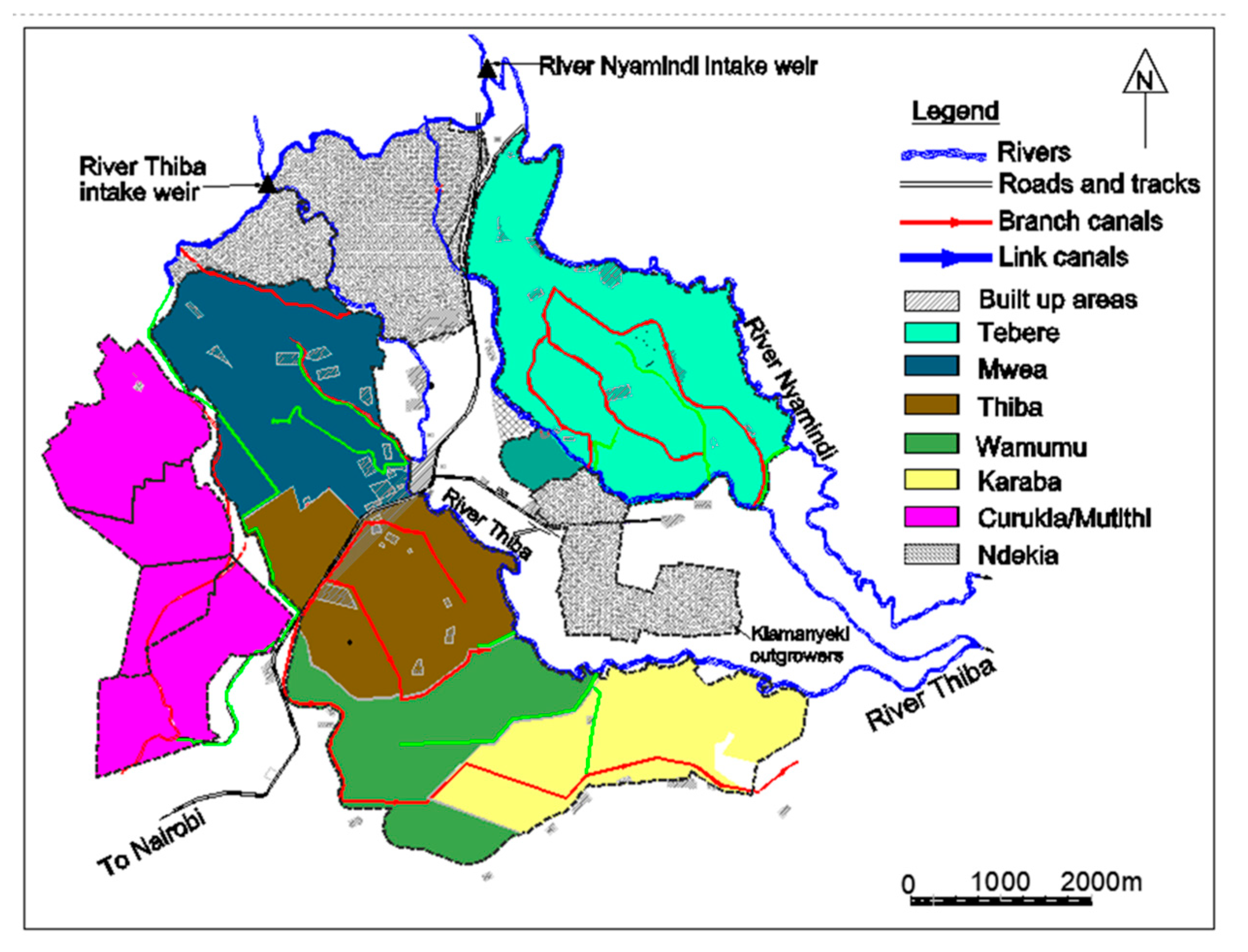
Figure 3.
Soil Water Assessment Tool (SWAT) model study area (a) topography map; (b) land use map; (c) soil map.
Figure 3.
Soil Water Assessment Tool (SWAT) model study area (a) topography map; (b) land use map; (c) soil map.

Figure 4.
Irrigation water requirements for the 2013–2016 seasons.

Figure 5.
SWAT model calibration and validation.
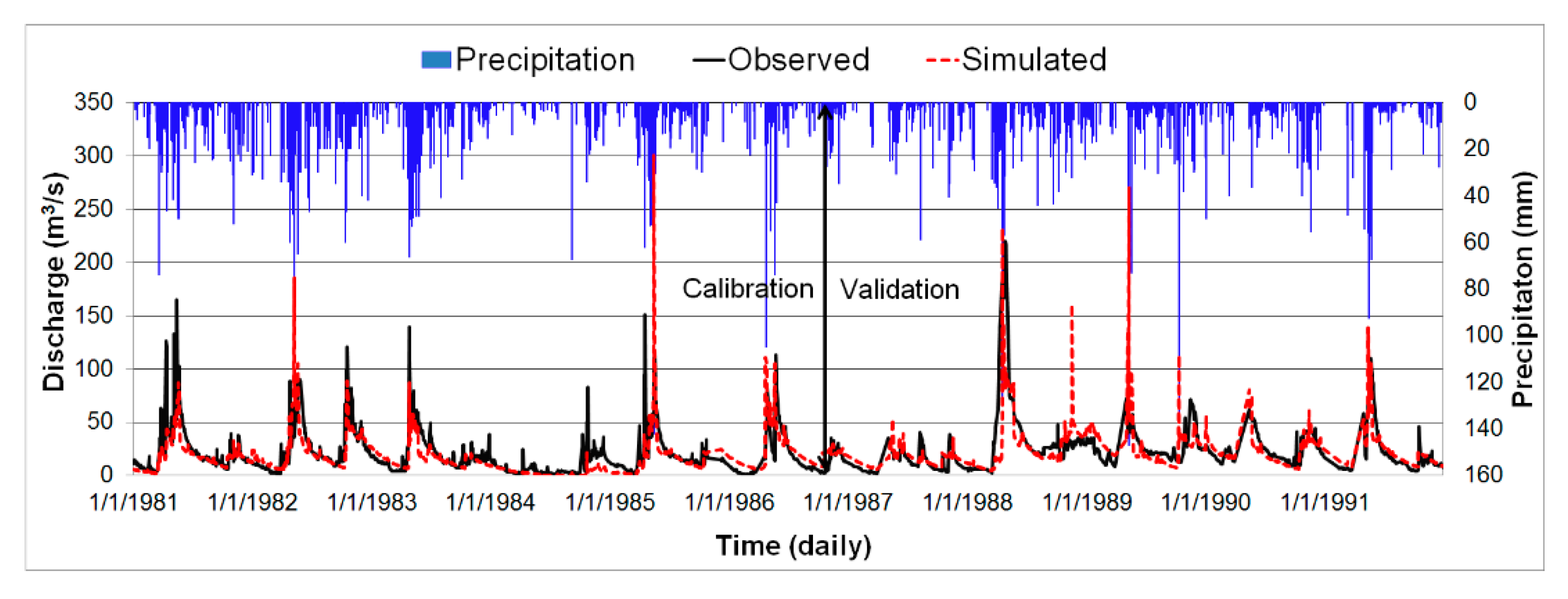
Figure 6.
Hydrology summary of the watershed simulation [63].
Figure 6.
Hydrology summary of the watershed simulation [63].

Figure 7.
Comparison of total available flow (historical simulation) with water demand (2013–2016).
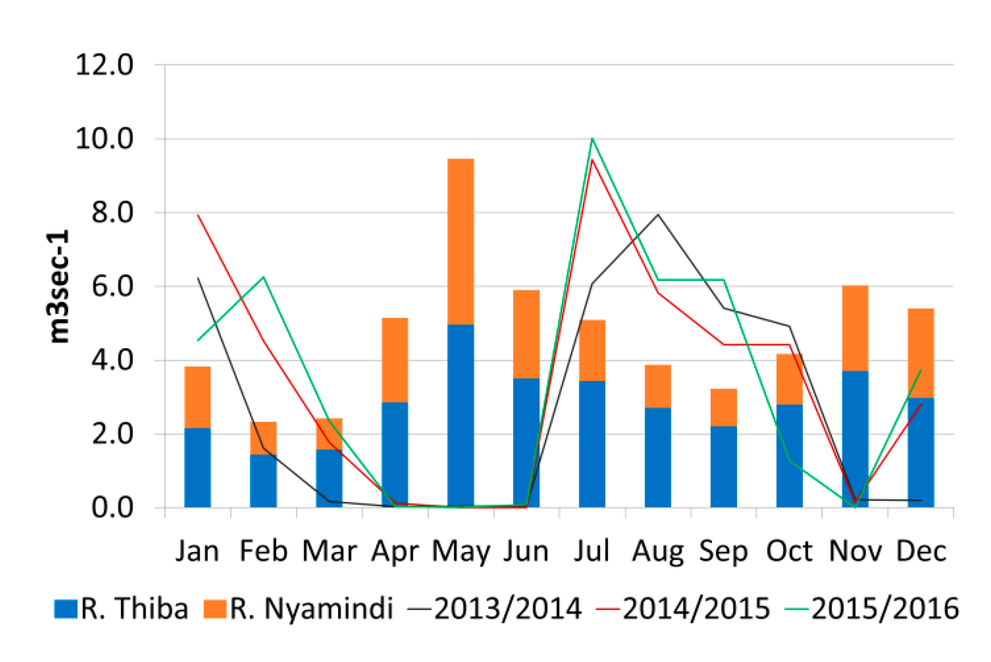
Figure 8.
RCP 2.6 Comparison of total available flow and irrigation water requirements during 2020–2060 and 2061–2099. (a) GCM 1 (2020–2060); (b) GCM 2 (2020–2060); (c) GCM 3 (2020–2060); (d) GCM 1 (2061–2099); (e) GCM 2 (2061–2099); (f) GCM 3 (2061–2099).
Figure 8.
RCP 2.6 Comparison of total available flow and irrigation water requirements during 2020–2060 and 2061–2099. (a) GCM 1 (2020–2060); (b) GCM 2 (2020–2060); (c) GCM 3 (2020–2060); (d) GCM 1 (2061–2099); (e) GCM 2 (2061–2099); (f) GCM 3 (2061–2099).

Figure 9.
RCP 4.5 Comparison of total available flow and irrigation water requirements during 2020–2060 and 2061–2099. (a) GCM 1 (2020–2060); (b) GCM 2 (2020–2060); (c) GCM 3 (2020–2060); (d) GCM 1 (2061–2099); (e) GCM 2 (2061–2099); (f) GCM 3 (2061–2099).
Figure 9.
RCP 4.5 Comparison of total available flow and irrigation water requirements during 2020–2060 and 2061–2099. (a) GCM 1 (2020–2060); (b) GCM 2 (2020–2060); (c) GCM 3 (2020–2060); (d) GCM 1 (2061–2099); (e) GCM 2 (2061–2099); (f) GCM 3 (2061–2099).

Figure 10.
RCP 6.0 Comparison of total available flow and irrigation water requirements during 2020–2060 and 2061–2099. (a) GCM 1 (2020–2060); (b) GCM 2 (2020–2060); (c) GCM 3 (2020–2060); (d) GCM 1 (2061–2099); (e) GCM 2 (2061–2099); (f) GCM 3 (2061–2099).
Figure 10.
RCP 6.0 Comparison of total available flow and irrigation water requirements during 2020–2060 and 2061–2099. (a) GCM 1 (2020–2060); (b) GCM 2 (2020–2060); (c) GCM 3 (2020–2060); (d) GCM 1 (2061–2099); (e) GCM 2 (2061–2099); (f) GCM 3 (2061–2099).
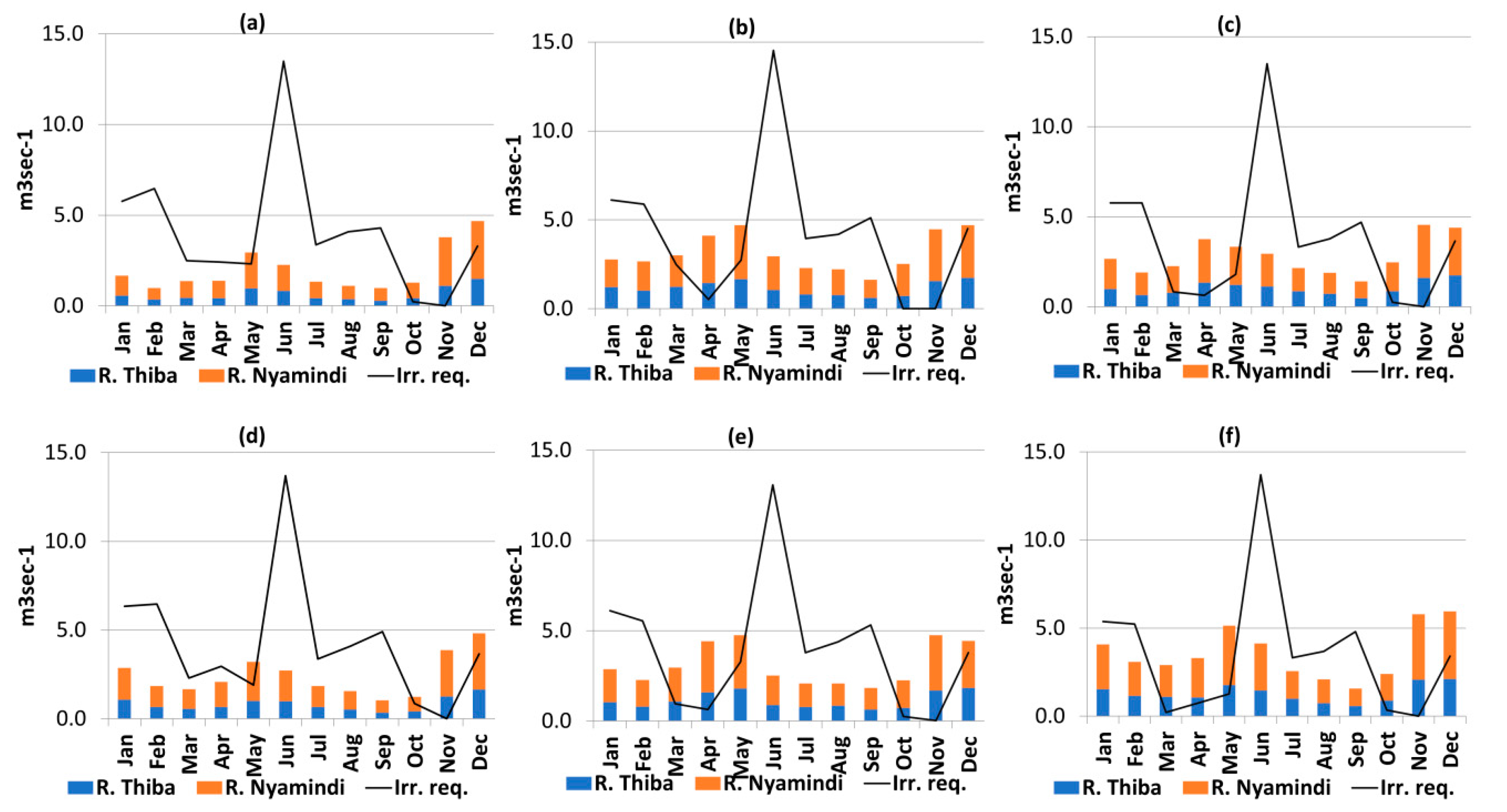
Figure 11.
RCP 8.5 Comparison of total available flow and irrigation water requirements during 2020–2060 and 2061–2099. (a) GCM 1 (2020–2060); (b) GCM 2 (2020–2060); (c) GCM 3 (2020–2060); (d) GCM 1 (2061–2099); (e) GCM 2 (2061–2099); (f) GCM 3 (2061–2099).
Figure 11.
RCP 8.5 Comparison of total available flow and irrigation water requirements during 2020–2060 and 2061–2099. (a) GCM 1 (2020–2060); (b) GCM 2 (2020–2060); (c) GCM 3 (2020–2060); (d) GCM 1 (2061–2099); (e) GCM 2 (2061–2099); (f) GCM 3 (2061–2099).

Table 1.
Summary of Thiba and Tebere systems, blocks and watershed area.
| System | Block | Gross Area (Hectares) | Total Watershed Area for This Study |
|---|---|---|---|
| Thiba | Mwea | 1681 | 1545 km² |
| Thiba | 1426 | ||
| Wamumu | 1445 | ||
| Karaba | 1325 | ||
| Curukia/Mutithi | 2804 | ||
| Tebere | Tebere | 2625 | |
| Ndekia | 2439 |
Table 2.
Comparison of existing and proposed cropping patterns.
| Jan | Feb | Mar | Apr | May | Jun | Jul | Aug | Sep | Oct | Nov | Dec | |
|---|---|---|---|---|---|---|---|---|---|---|---|---|
| Existing pattern | Ratoon rice | Rotavation | Transplanting | Main rice crop | ||||||||
| Proposed pattern | Ratoon rice/short rain upland crops | Long rain upland crops | Main rice crop | Ratoon rice/short rain upland crops | ||||||||
Table 3.
Comparison of irrigation areas in groups, blocks and years of existing cropping patterns.
| Cropping Patterns | Year | Tebere (Ha) | Mwea (Ha) | Thiba (Ha) | Wamumu (Ha) | Karaba (Ha) | Curukia (Ha) | Ndekia (Ha) | Total Area (ha) |
|---|---|---|---|---|---|---|---|---|---|
| Group 1 | 2013/2014 | 0 | 653 | 1183 | 681 | 712 | 445 | 0 | 3674 |
| 2014/2015 | 1363 | 909 | 1017 | 679 | 758 | 1021 | 0 | 5747 | |
| 2015/2016 | 1363 | 976 | 1017 | 680 | 809 | 1021 | 0 | 5866 | |
| Group 2 | 2013/2014 | 1670 | 633 | 0 | 487 | 420 | 457 | 439 | 4106 |
| 2014/2015 | 500 | 377 | 165 | 488 | 373 | 0 | 439 | 2342 | |
| 2015/2016 | 583 | 447 | 165 | 536 | 428 | 0 | 439 | 2598 | |
| Group 3 | 2013/2014 | 110 | 0 | 0 | 0 | 0 | 0 | 0 | 110 |
| 2014/2015 | 0 | 0 | 0 | 0 | 0 | 0 | 0 | 0 | |
| 2015/2016 | 0 | 0 | 0 | 0 | 0 | 0 | 439 | 439 |
Table 4.
Irrigation areas and crops of the proposed cropping pattern.
| Irrigation Areas | Short Rain Rice and Rice Ratoon | Short Rain Upland | Long Rain Rice | Long Rain Upland |
|---|---|---|---|---|
| Tebere system | 1800 | 300 | 0 | 1400 |
| Thiba system | 4980 | 200 | 0 | 4900 |
| New extension areas | 1127 | 1078 | 0 | 2205 |
| Total area (ha) | 7907 | 1578 | 0 | 8050 |
Table 5.
Observed weather stations, intakes and watershed outlet information.
| ID | Description | Latitude | Longitude | Elevation (m) |
|---|---|---|---|---|
| 1 | Castle Forest station | 0°24.498′ S | 37°18.64′ E | 1918 |
| 2 | Embu station | 0°30′ S | 37°27′ E | 1493 |
| 3 | River Nyamindi intake | 0°36.274′ S | 37°22.135′ E | 1210 |
| 4 | River Thiba intake | 0°37.532′ S | 37°19.212′ E | 1203 |
| 5 | MIAD station | 0°39.384′ S | 37°17.40′ E | 1159 |
| 6 | Watershed outlet (RGS4DD02) | 0°43.92′ S | 37°30.360′ E | 1056 |
Table 6.
Categorization of water scarcity by Water Scarcity Index (WSI).
| Index | Category |
|---|---|
| >1 | Overexploited |
| 0.6 ≤ WSI < 1 | Heavily exploited |
| 0.3 ≤ WSI < 0.6 | Moderately exploited |
| WSI < 0.3 | Slightly exploited |
Table 7.
Global Circulation Models with Representative Concentration Pathways (RCPs) and periods.
| Model | Scenarios | Period | |
|---|---|---|---|
| GFDL-ESM2M | RCP (2.6, 4.5, 6.0, 8.5) | Historical | 1950–2005 |
| Future | 2006–2099 | ||
| HadGEM2-ES | RCP (2.6, 4.5, 6.0, 8.5) | Historical | 1950–2005 |
| Future | 2006–2099 | ||
| NoerESM1-M | RCP (2.6, 4.5, 6.0, 8.5) | Historical Future | 1950–2005 |
| 2006–2099 |
Table 8.
General Circulation Model (GCM) stations information.
| Station | Latitude | Longitude | Elevation (m) |
|---|---|---|---|
| 435179 | 0°37.50′ S | 37°22.50′ E | 1186 |
| 435180 | 0°22.50′ S | 37°22.50′ E | 1958 |
| 436179 | 0°37.50′ S | 37°37.50′ E | 1194 |
| 436180 | 0°22.50′ S | 37°37.50′ E | 1452 |
Table 9.
SWAT model calibration objective functions.
| Nash–Sutcliffe Efficiency, NSE | |
|---|---|
| Calibration | Validation |
| 0.55 | 0.52 |
| Percent Bias, PBIAS | |
| −0.9% | −1.3% |
Table 10.
Model calibration parameters.
| Parameter_Name | Description | Fitted_Value | Min_Value | Max_Value |
|---|---|---|---|---|
| 1: R__CN2.mgt | SCS runoff curve number | 35 | 35 | 98 |
| 2: V__GW_DELAY.gw | Groundwater delay (days) | 19.049999 | 0 | 30 |
| 3: V__GWQMN.gw | Threshold depth of water in the shallow aquifer required for return flow to occur (mm) | 2227.5 | 2000 | 2500 |
| 4: V__SOL_AWC.sol | Available water capacity of the soil layer | 0.5203 | 0.4 | 0.7 |
| 5: V__ALPHA_BF.gw | Base flow alpha factor (days) | 0.7397 | 0.5 | 0.8 |
Note: R_ means relatively changing value; V_ means replacing with new value.
Table 11.
RCP 2.6 Future Water Stress Index (WSI) estimations.
| Period | GCM | Jan | Feb | Mar | Apr | May | Jun | Jul | Aug | Sep | Oct | Nov | Dec |
|---|---|---|---|---|---|---|---|---|---|---|---|---|---|
| 2020–2060 | 1 | 1.95 | 3.83 | 1.06 | 1.34 | 0.81 | 5.08 | 2.47 | 3.29 | 4.04 | 0.19 | 0.00 | 0.78 |
| 2 | 3.24 | 5.16 | 1.57 | 0.88 | 1.24 | 6.58 | 2.79 | 3.38 | 7.04 | 0.03 | 0.00 | 2.04 | |
| 3 | 1.70 | 2.52 | 0.74 | 0.38 | 0.45 | 2.72 | 1.04 | 1.64 | 2.36 | 0.26 | 0.00 | 0.57 | |
| 2061–2099 | 1 | 2.70 | 3.58 | 2.32 | 1.98 | 0.89 | 6.14 | 3.00 | 4.40 | 6.60 | 1.32 | 0.00 | 0.74 |
| 2 | 2.49 | 3.79 | 0.62 | 0.63 | 0.90 | 6.16 | 1.93 | 2.50 | 4.70 | 0.64 | 0.00 | 1.44 | |
| 3 | 1.62 | 2.52 | 0.16 | 0.16 | 0.23 | 3.13 | 1.06 | 1.48 | 2.83 | 0.43 | 0.00 | 0.58 |
Table 12.
RCP 4.5 Future Water Stress Index (WSI) estimations.
| Period | GCM | Jan | Feb | Mar | Apr | May | Jun | Jul | Aug | Sep | Oct | Nov | Dec |
|---|---|---|---|---|---|---|---|---|---|---|---|---|---|
| 2020–2060 | 1 | 2.13 | 3.85 | 2.64 | 1.89 | 0.95 | 6.06 | 2.75 | 3.15 | 5.87 | 0.73 | 0.00 | 0.65 |
| 2 | 3.74 | 5.20 | 0.64 | 0.17 | 0.74 | 5.98 | 1.87 | 2.78 | 4.98 | 0.11 | 0.00 | 2.42 | |
| 3 | 2.51 | 3.91 | 0.63 | 0.38 | 0.33 | 3.95 | 1.56 | 2.64 | 2.99 | 0.06 | 0.00 | 0.92 | |
| 2061–2099 | 1 | 2.14 | 2.57 | 1.82 | 1.63 | 0.55 | 6.82 | 2.70 | 2.86 | 5.83 | 0.77 | 0.00 | 0.55 |
| 2 | 2.42 | 2.57 | 0.46 | 0.83 | 0.67 | 6.10 | 2.18 | 2.61 | 4.70 | 0.24 | 0.00 | 1.33 | |
| 3 | 2.10 | 2.72 | 0.20 | 0.36 | 0.43 | 4.32 | 1.59 | 2.32 | 4.21 | 0.71 | 0.00 | 0.83 |
Table 13.
RCP 6.0 Future Water Stress Index (WSI) estimations.
| Period | GCM | Jan | Feb | Mar | Apr | May | Jun | Jul | Aug | Sep | Oct | Nov | Dec |
|---|---|---|---|---|---|---|---|---|---|---|---|---|---|
| 2020–2060 | 1 | 3.47 | 6.54 | 1.83 | 1.76 | 0.79 | 5.98 | 2.52 | 3.71 | 4.36 | 0.18 | 0.00 | 0.70 |
| 2 | 2.20 | 2.21 | 0.83 | 0.13 | 0.58 | 4.93 | 1.73 | 1.88 | 3.14 | 0.01 | 0.00 | 0.96 | |
| 3 | 2.16 | 3.03 | 0.37 | 0.17 | 0.54 | 4.58 | 1.54 | 2.00 | 3.33 | 0.10 | 0.00 | 0.83 | |
| 2061–2099 | 1 | 2.22 | 3.52 | 1.37 | 1.42 | 0.59 | 5.04 | 1.83 | 2.62 | 4.70 | 0.69 | 0.00 | 0.76 |
| 2 | 2.13 | 2.43 | 0.32 | 0.14 | 0.69 | 5.19 | 1.81 | 2.10 | 2.89 | 0.11 | 0.00 | 0.85 | |
| 3 | 1.32 | 1.69 | 0.07 | 0.22 | 0.25 | 3.31 | 1.30 | 1.77 | 3.07 | 0.14 | 0.00 | 0.57 |
Table 14.
RCP 8.5 Future Water Stress Index (WSI) estimations.
| Period | GCM | Jan | Feb | Mar | Apr | May | Jun | Jul | Aug | Sep | Oct | Nov | Dec |
|---|---|---|---|---|---|---|---|---|---|---|---|---|---|
| 2020–2060 | 1 | 4.00 | 4.33 | 1.22 | 0.98 | 0.38 | 2.63 | 1.02 | 1.45 | 1.87 | 0.12 | 0.00 | 0.91 |
| 2 | 3.97 | 4.13 | 1.09 | 0.81 | 0.98 | 5.54 | 2.20 | 2.72 | 3.46 | 0.01 | 0.00 | 2.13 | |
| 3 | 2.02 | 2.77 | 0.89 | 0.48 | 0.36 | 4.31 | 1.76 | 2.35 | 3.44 | 0.01 | 0.00 | 0.62 | |
| 2061–2099 | 1 | 3.02 | 4.34 | 0.97 | 0.83 | 0.43 | 2.70 | 0.88 | 1.47 | 2.59 | 0.45 | 0.00 | 0.94 |
| 2 | 1.99 | 1.74 | 0.80 | 0.91 | 0.26 | 4.76 | 1.78 | 2.44 | 4.60 | 0.15 | 0.00 | 0.79 | |
| 3 | 2.02 | 2.89 | 0.57 | 0.98 | 0.67 | 4.48 | 1.71 | 2.27 | 4.39 | 0.12 | 0.00 | 0.77 |
© 2020 by the authors. Licensee MDPI, Basel, Switzerland. This article is an open access article distributed under the terms and conditions of the Creative Commons Attribution (CC BY) license (http://creativecommons.org/licenses/by/4.0/).
Share and Cite
MDPI and ACS Style
Akoko, G.; Kato, T.; Tu, L.H. Evaluation of Irrigation Water Resources Availability and Climate Change Impacts—A Case Study of Mwea Irrigation Scheme, Kenya. Water 2020, 12, 2330. https://doi.org/10.3390/w12092330
AMA Style
Akoko G, Kato T, Tu LH. Evaluation of Irrigation Water Resources Availability and Climate Change Impacts—A Case Study of Mwea Irrigation Scheme, Kenya. Water. 2020; 12(9):2330. https://doi.org/10.3390/w12092330
Chicago/Turabian StyleAkoko, George, Tasuku Kato, and Le Hoang Tu. 2020. "Evaluation of Irrigation Water Resources Availability and Climate Change Impacts—A Case Study of Mwea Irrigation Scheme, Kenya" Water 12, no. 9: 2330. https://doi.org/10.3390/w12092330
Note that from the first issue of 2016, this journal uses article numbers instead of page numbers. See further details here.