Numerical and Observational Analysis of the Hydro-Dynamical Variability in a Small Lake: The Case of Lake Zirahuén, México

 , , and
Abstract
1. Introduction
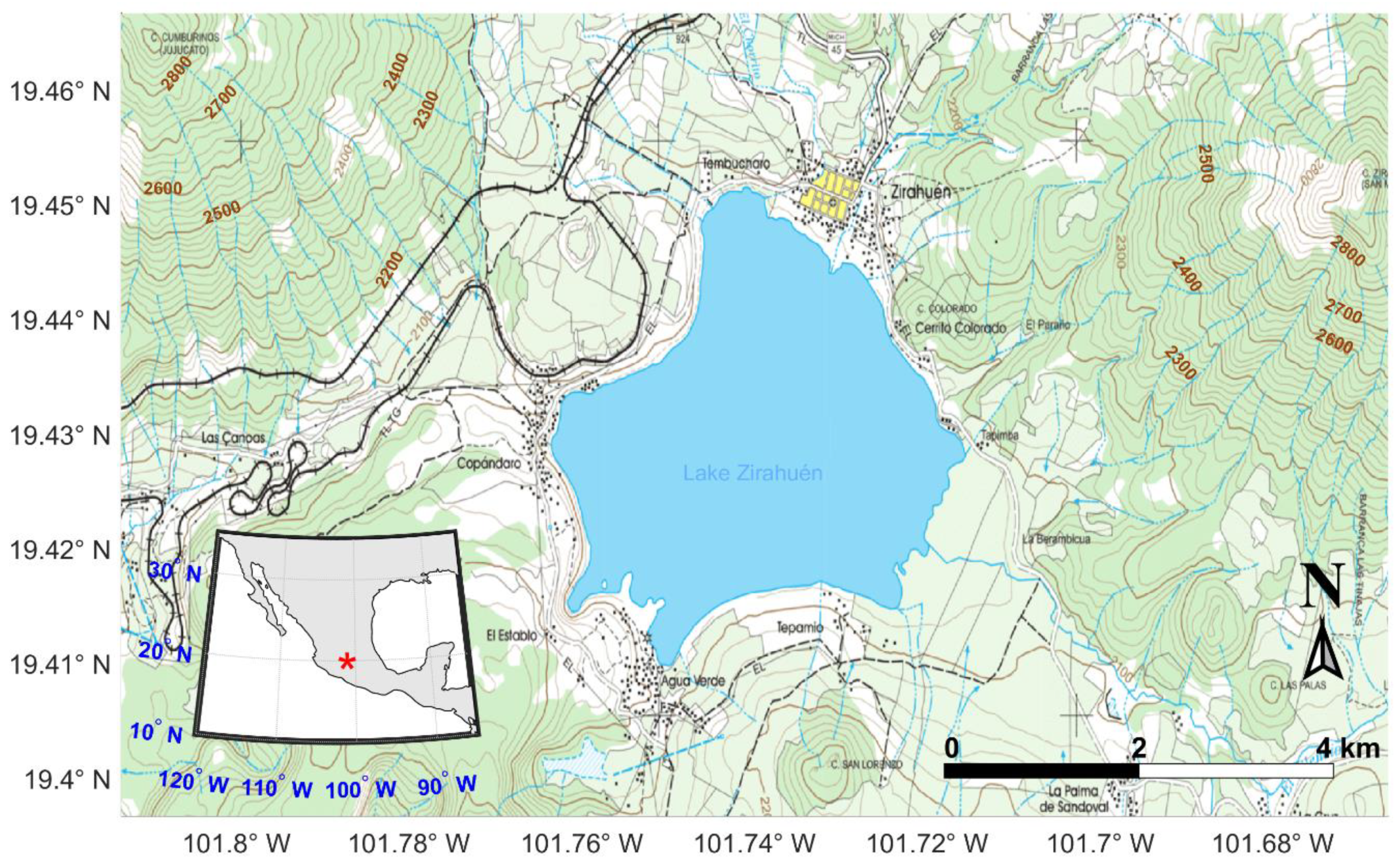
Study Area
2. Materials and Methods
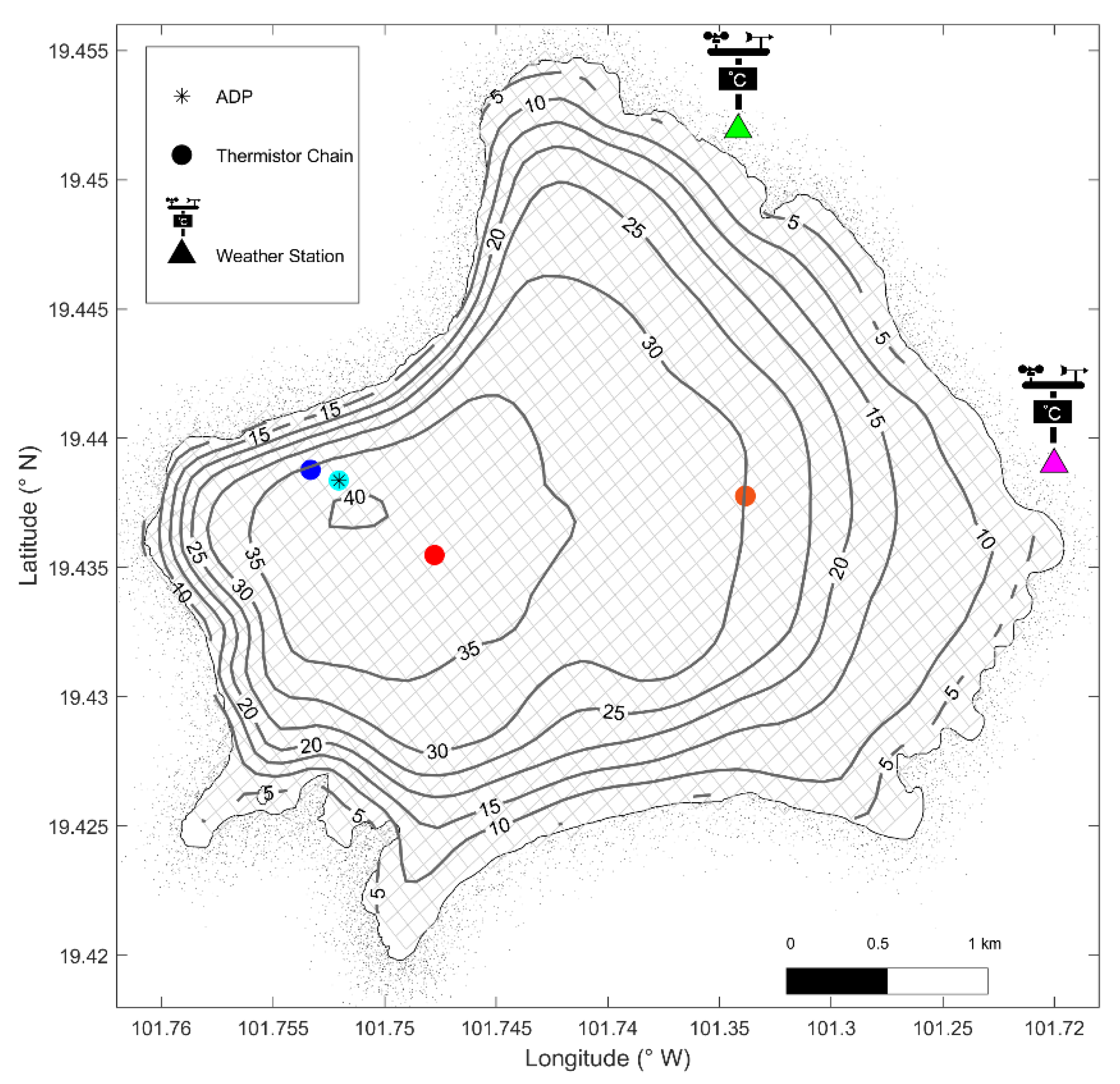
2.1. Field Campaigns of Measurements in 2018
2.1.1. Weather Station
2.1.2. CTD Casts and Thermistor Chains
2.1.3. Current Meter
2.1.4. Bathymetry and GPS
2.2. Numerical Model
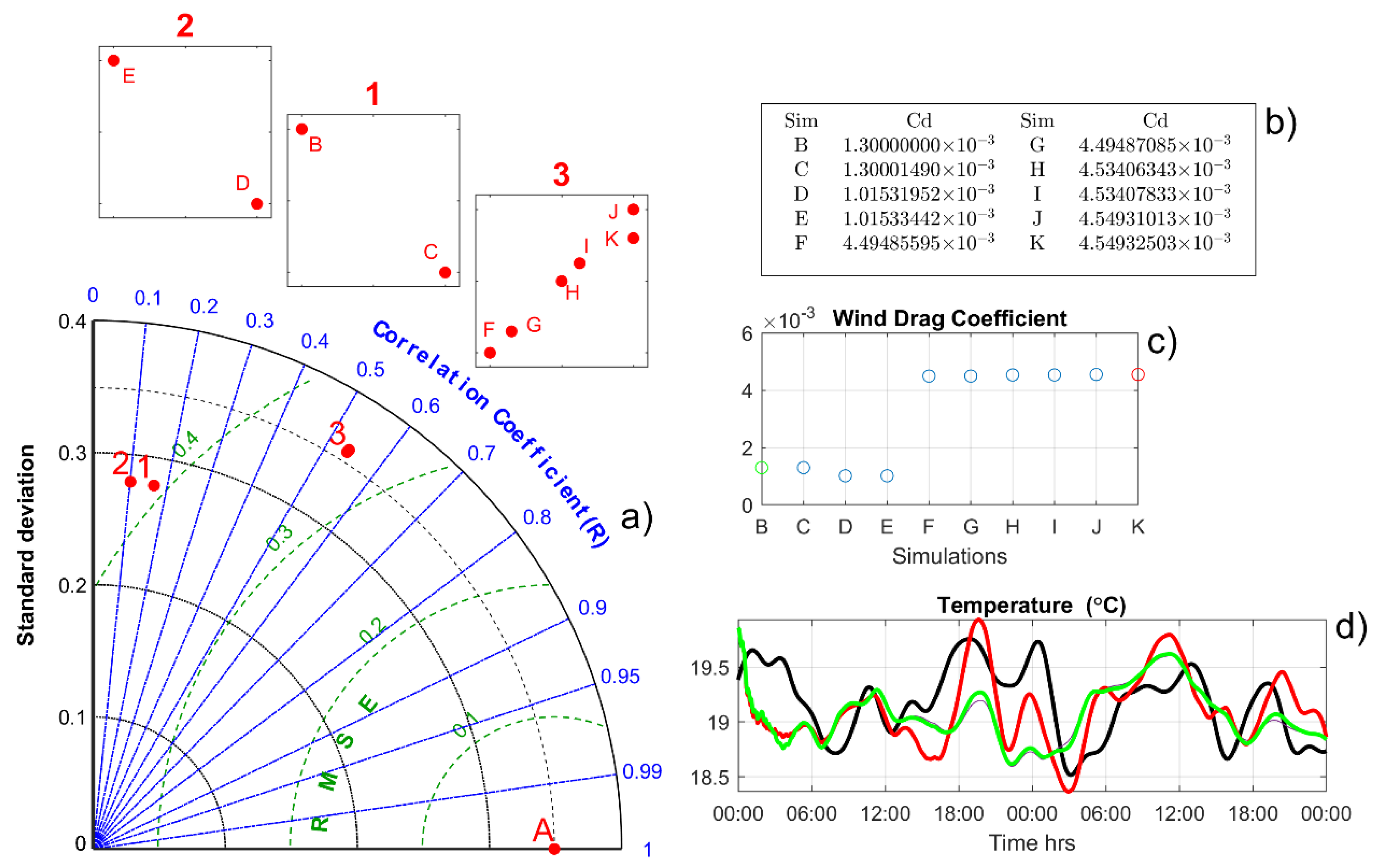
Model Calibration
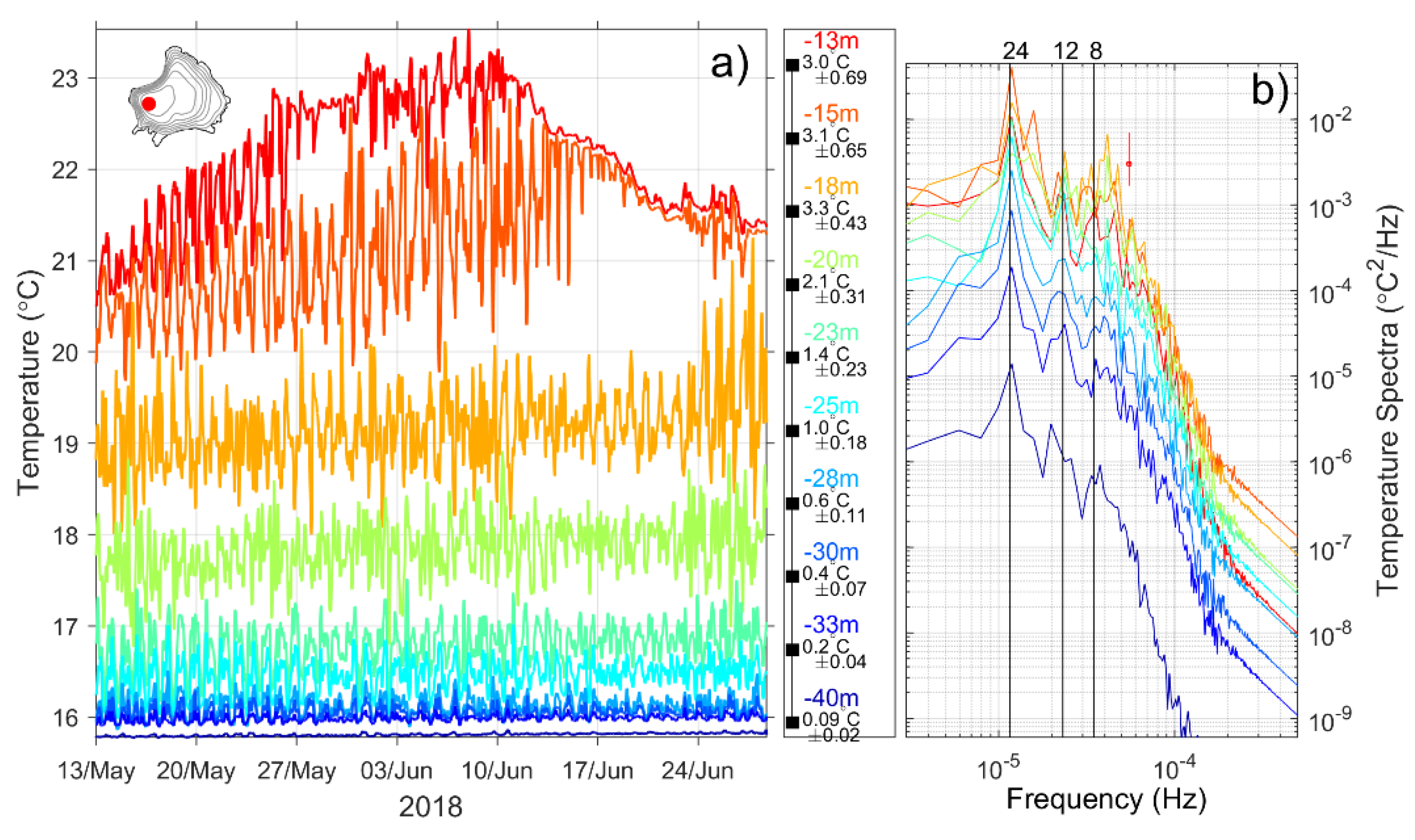
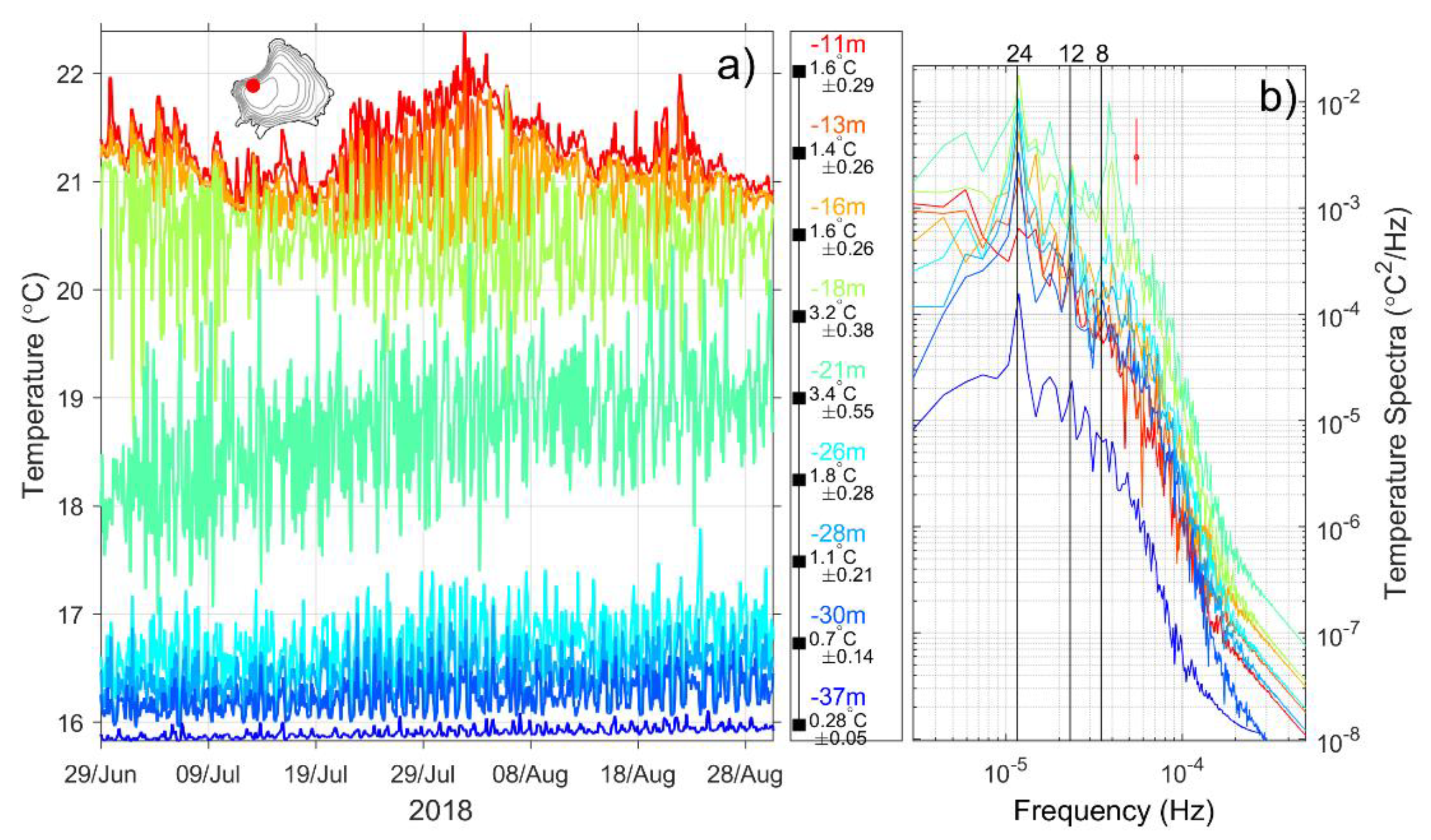
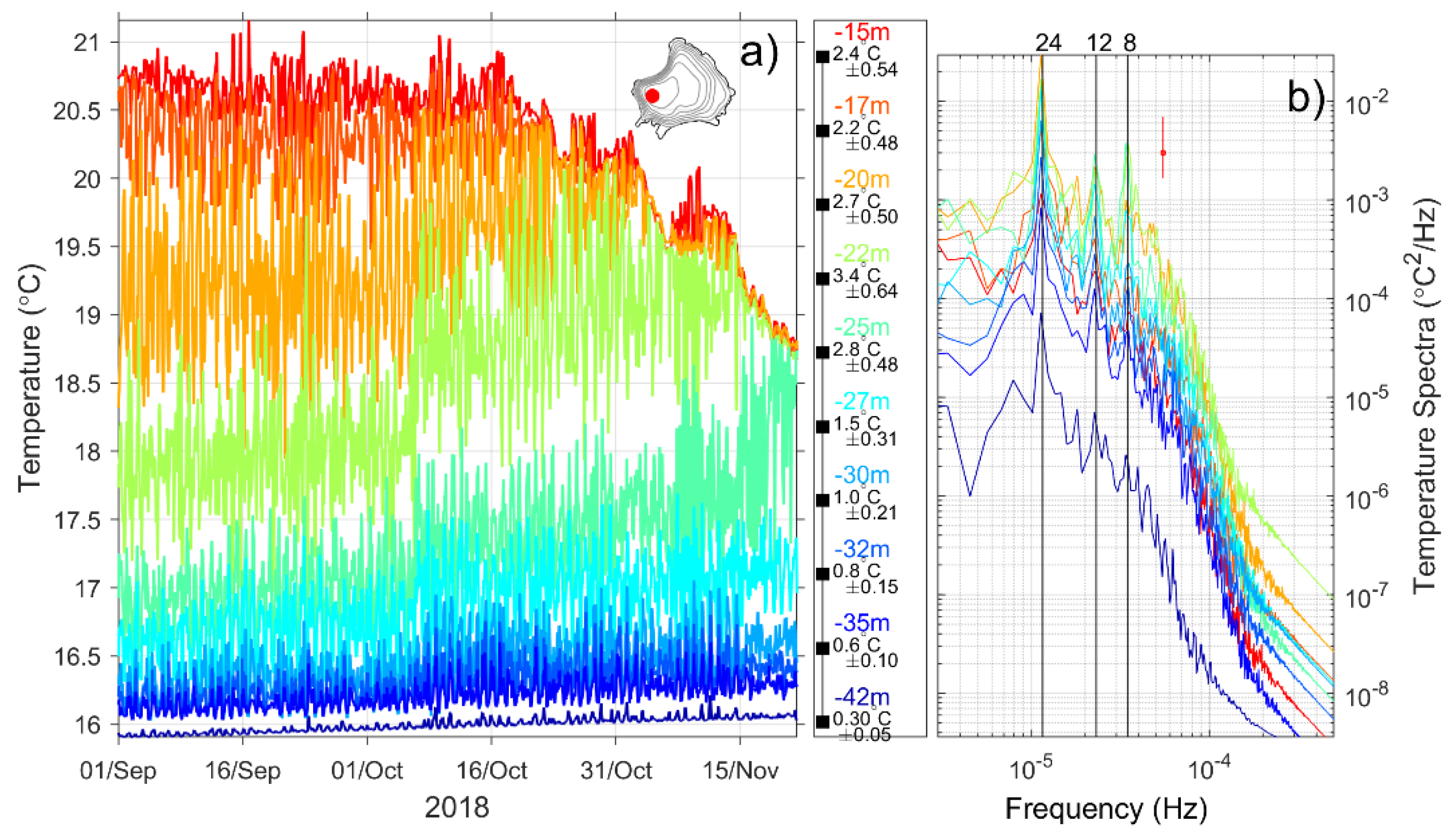
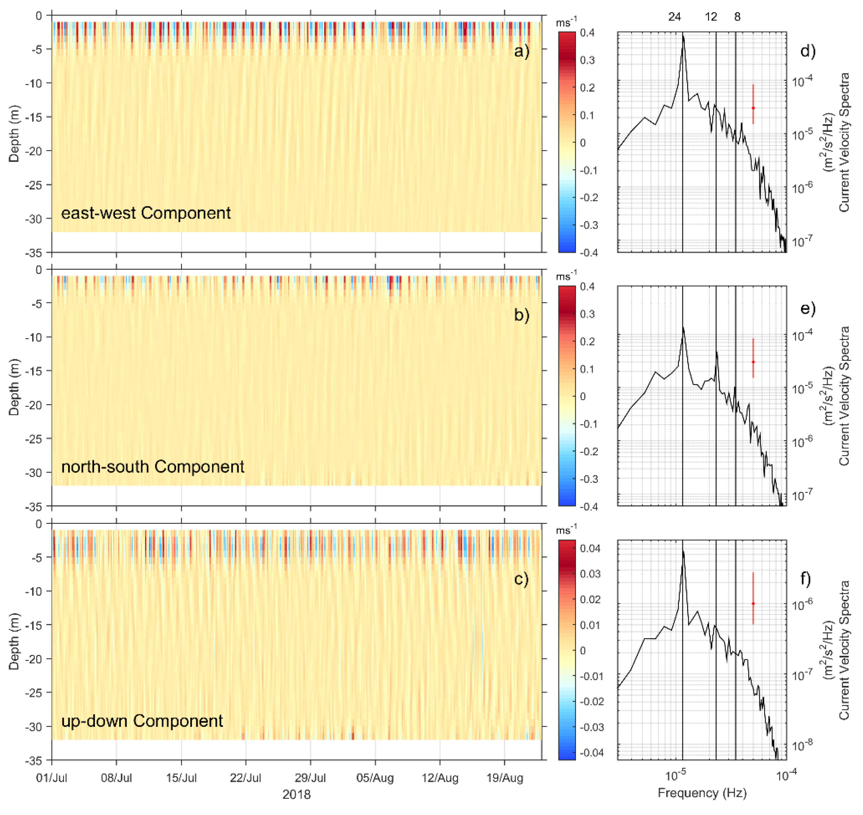
2.3. Spectral Analysis
2.4. Metrics to Evaluate the Performance of the Hydrodynamical Model
2.5. Normal Modes of Oscillation
3. Results and Discussion
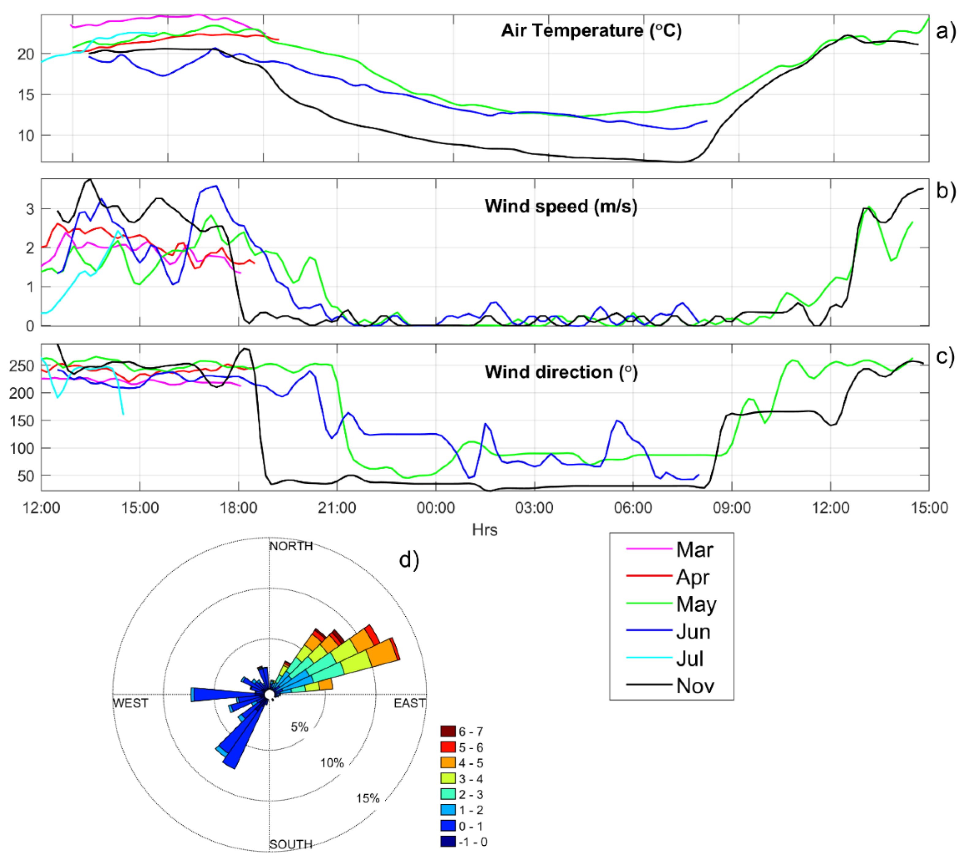
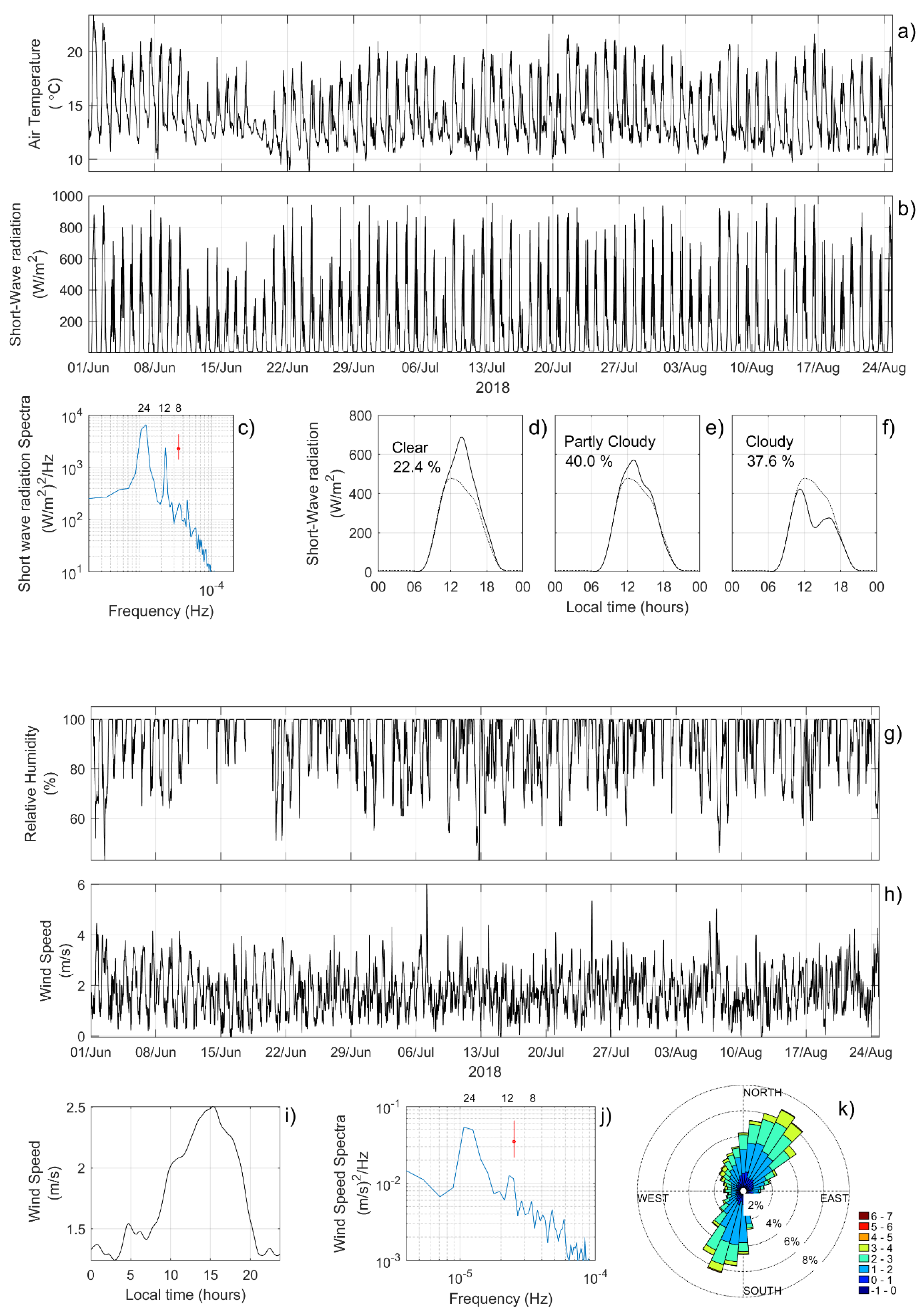
3.1. Weather Parameters
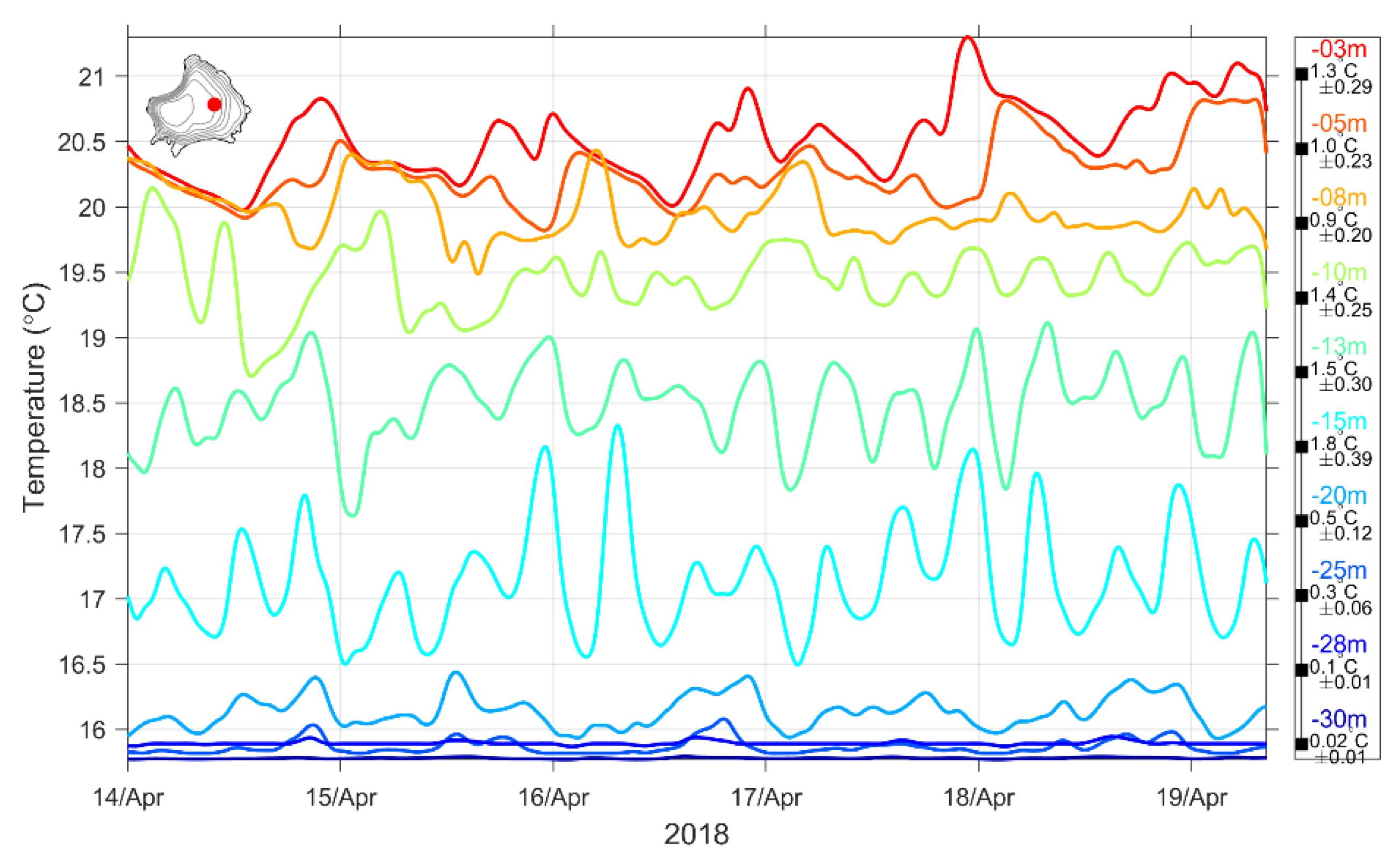
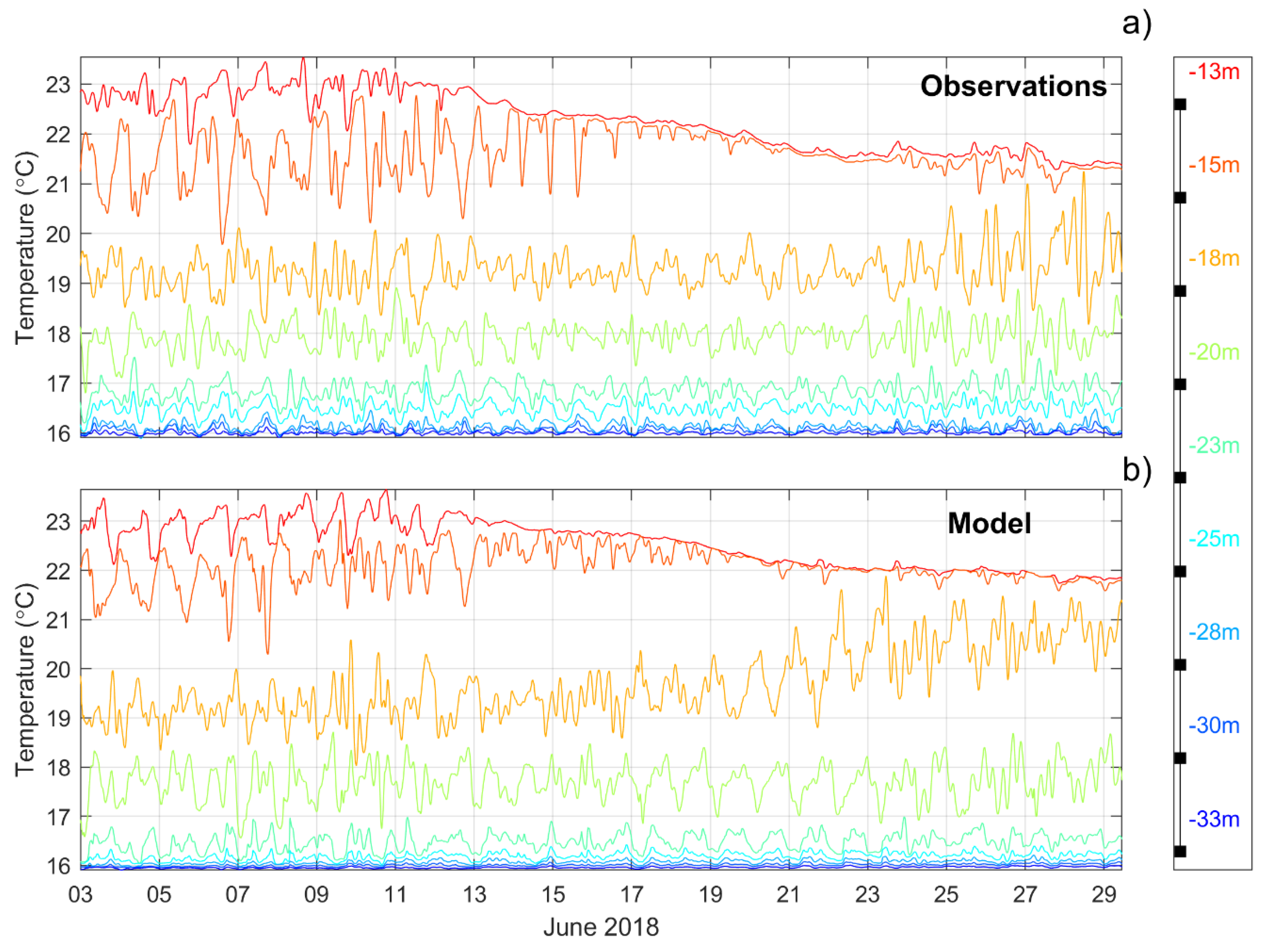
3.2. Hydrography from the Observational Thermistor Chain Data
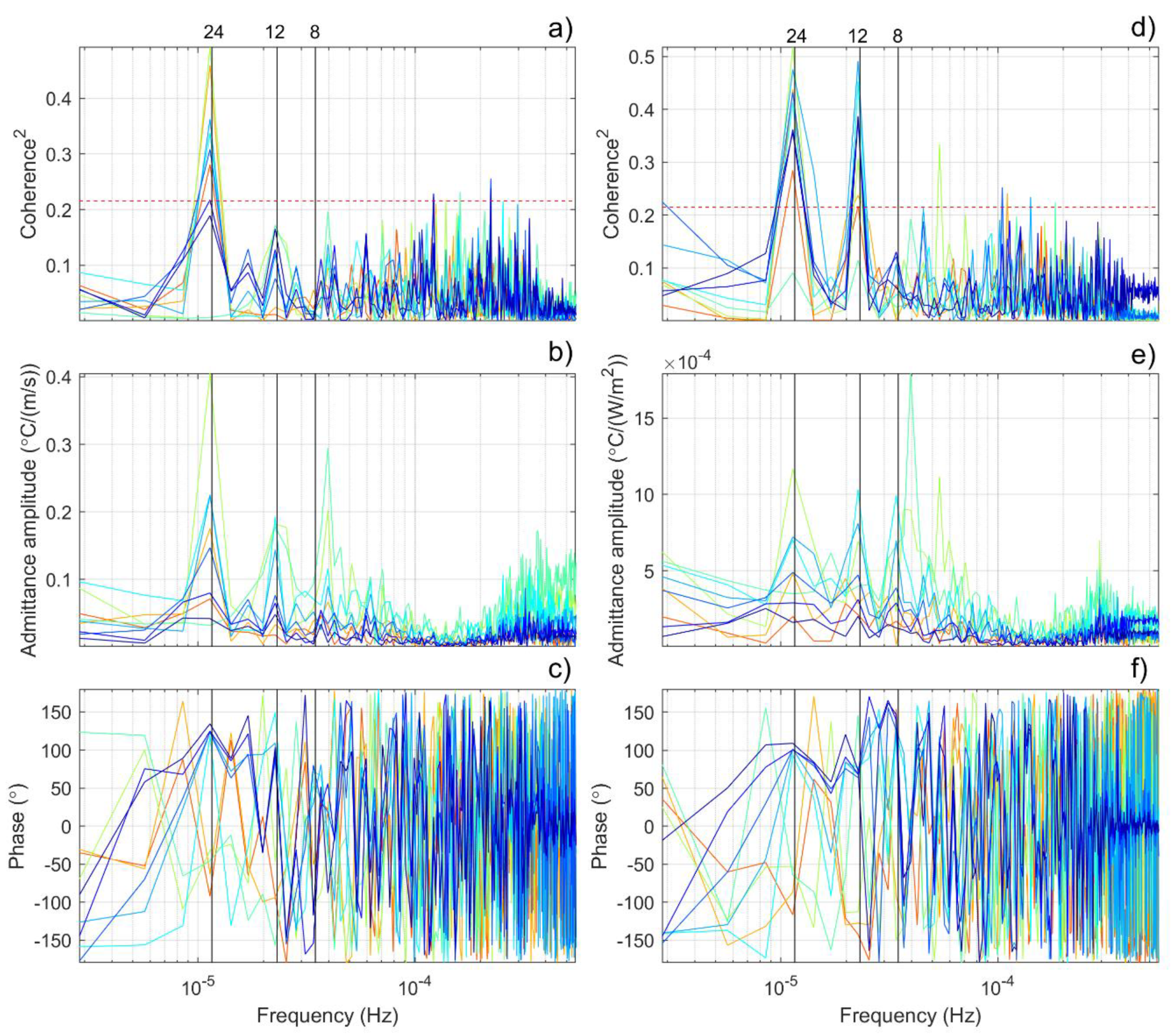
3.3. Response Transfer Functions
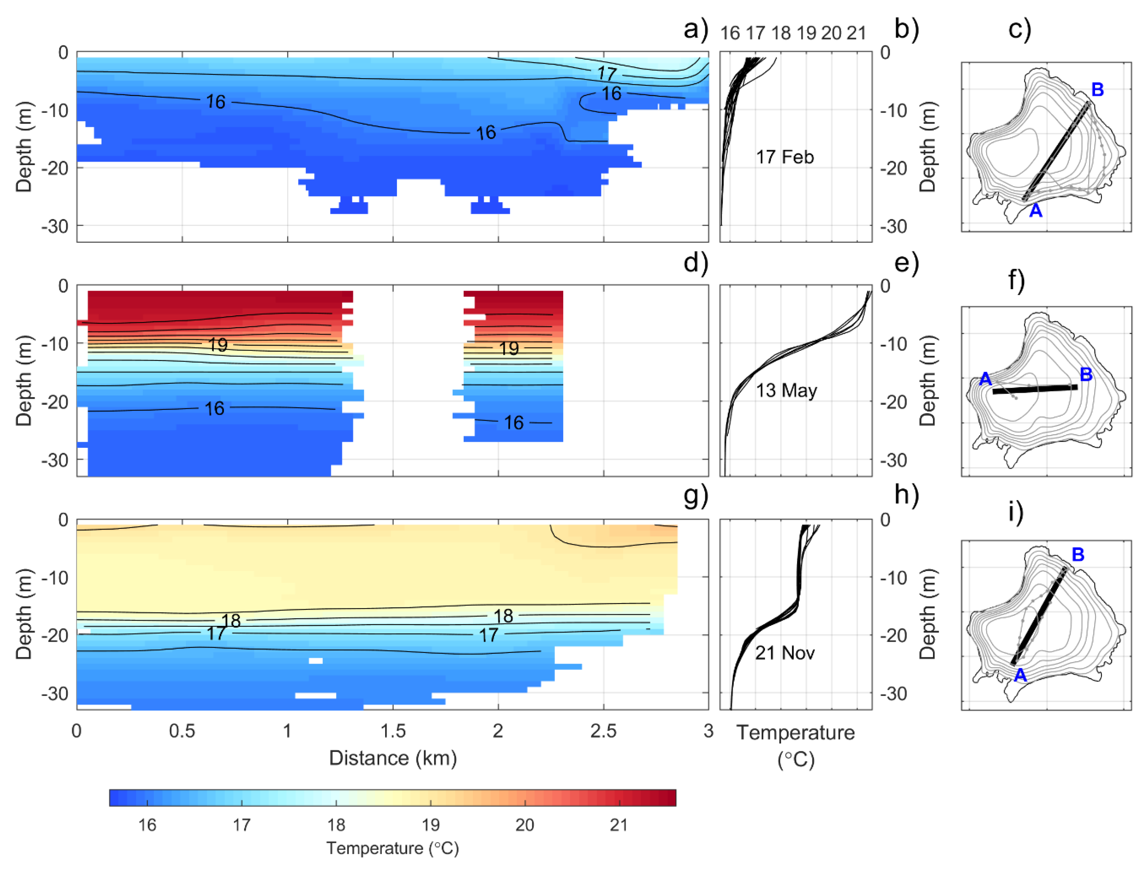
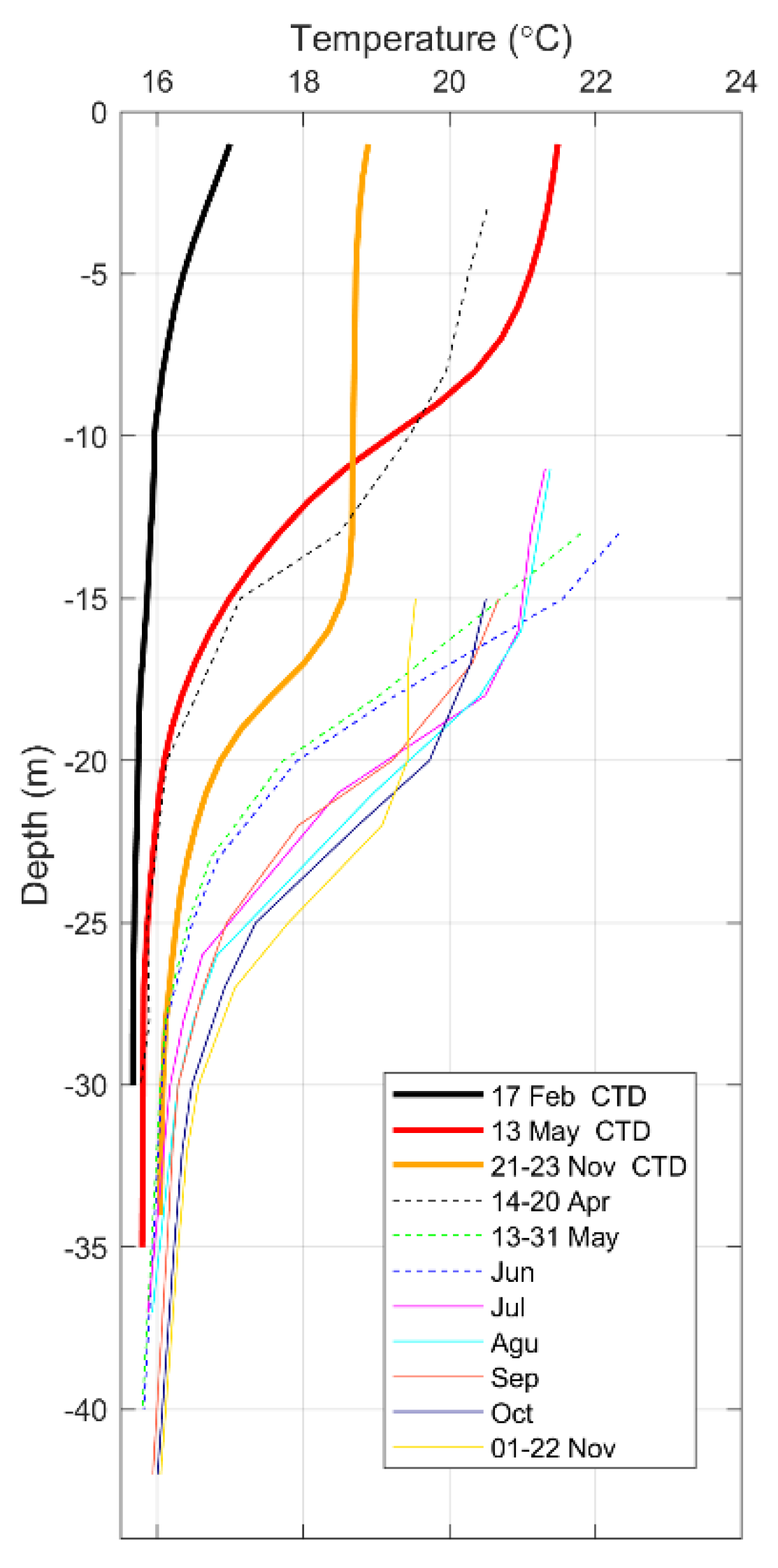
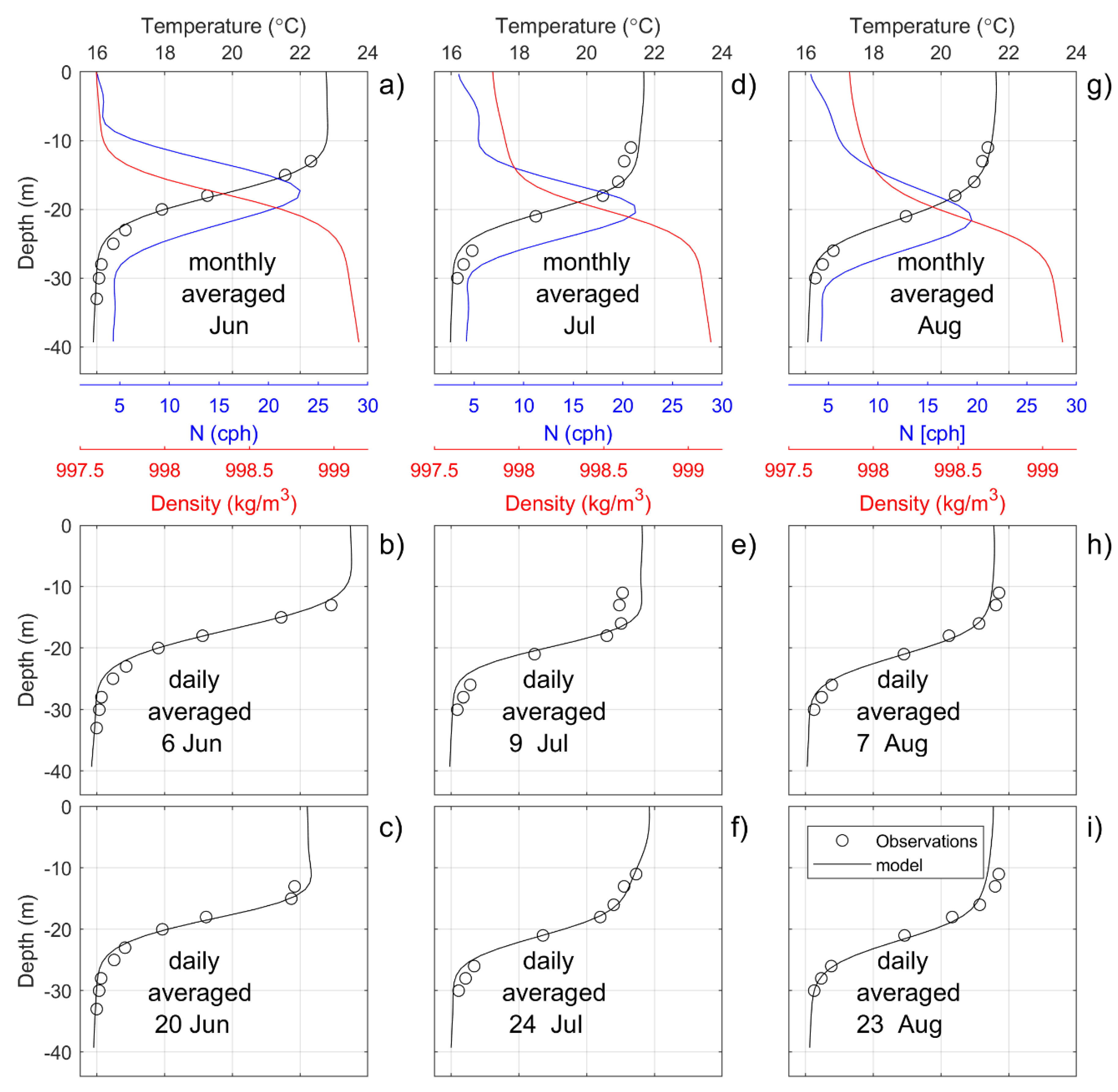
3.4. CTD Data
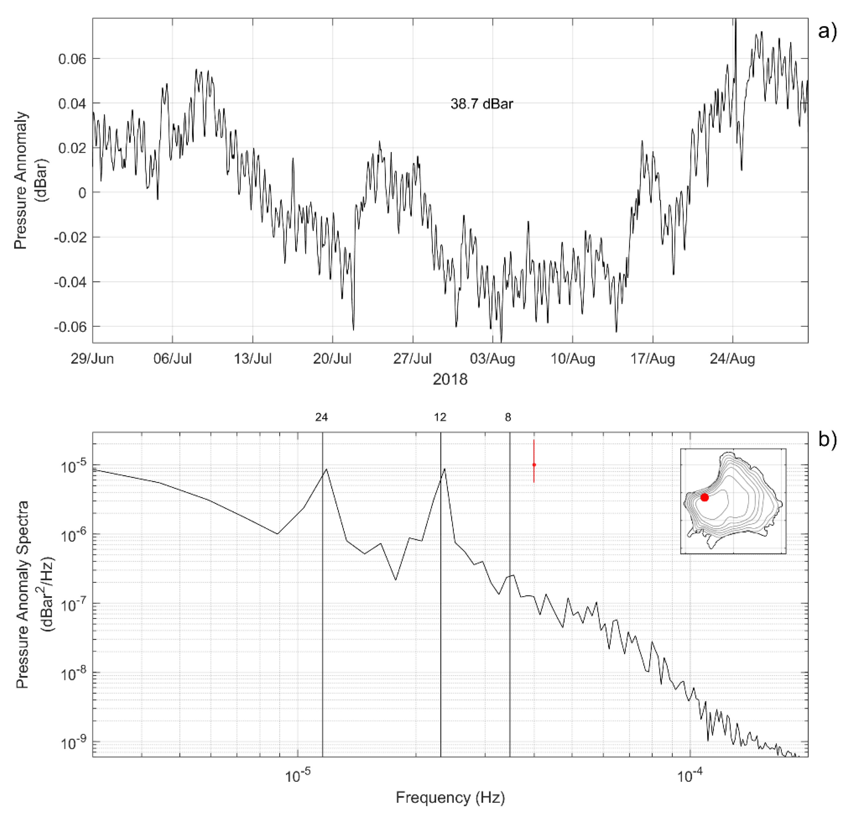
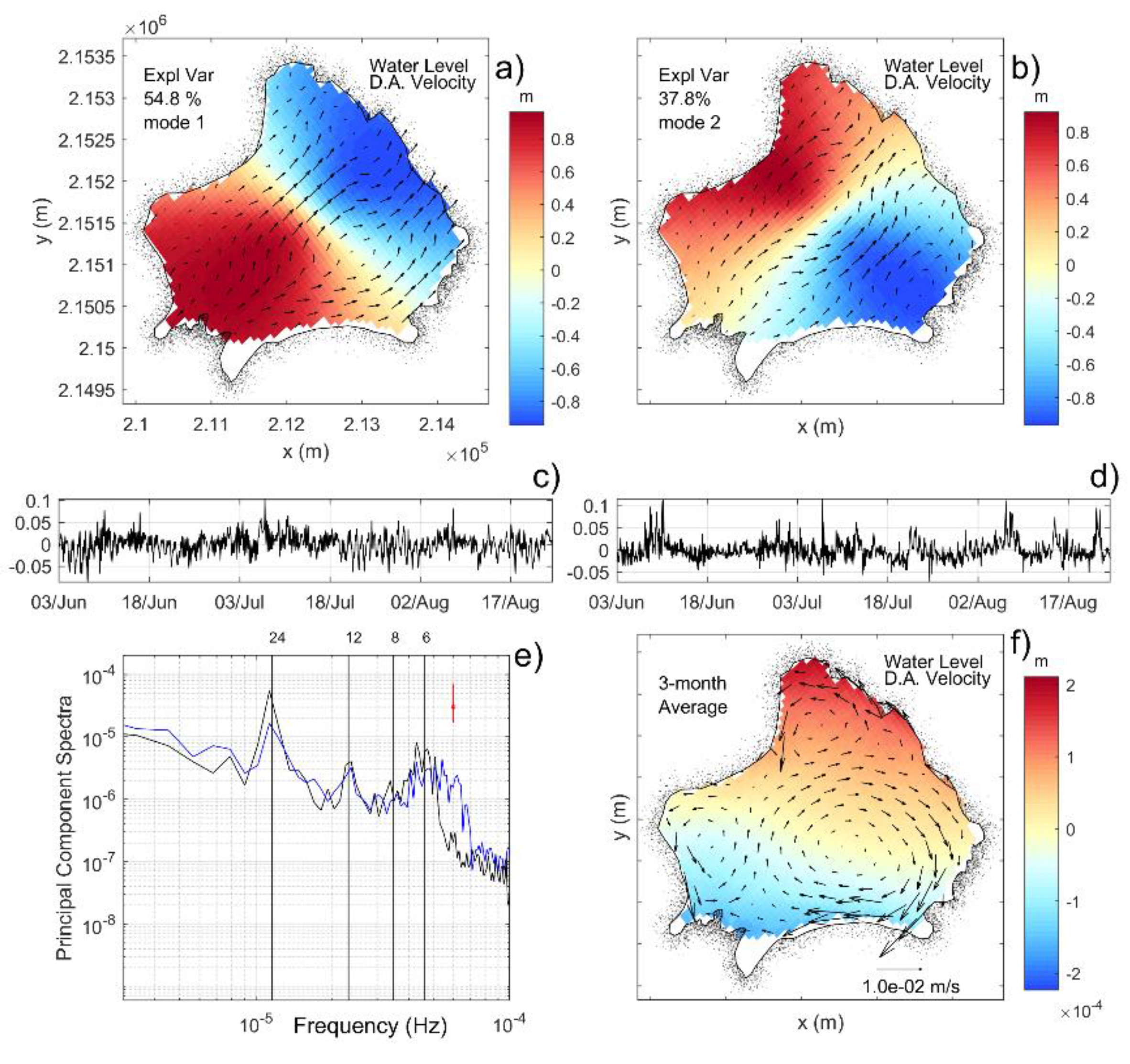
3.5. Water Level Chain
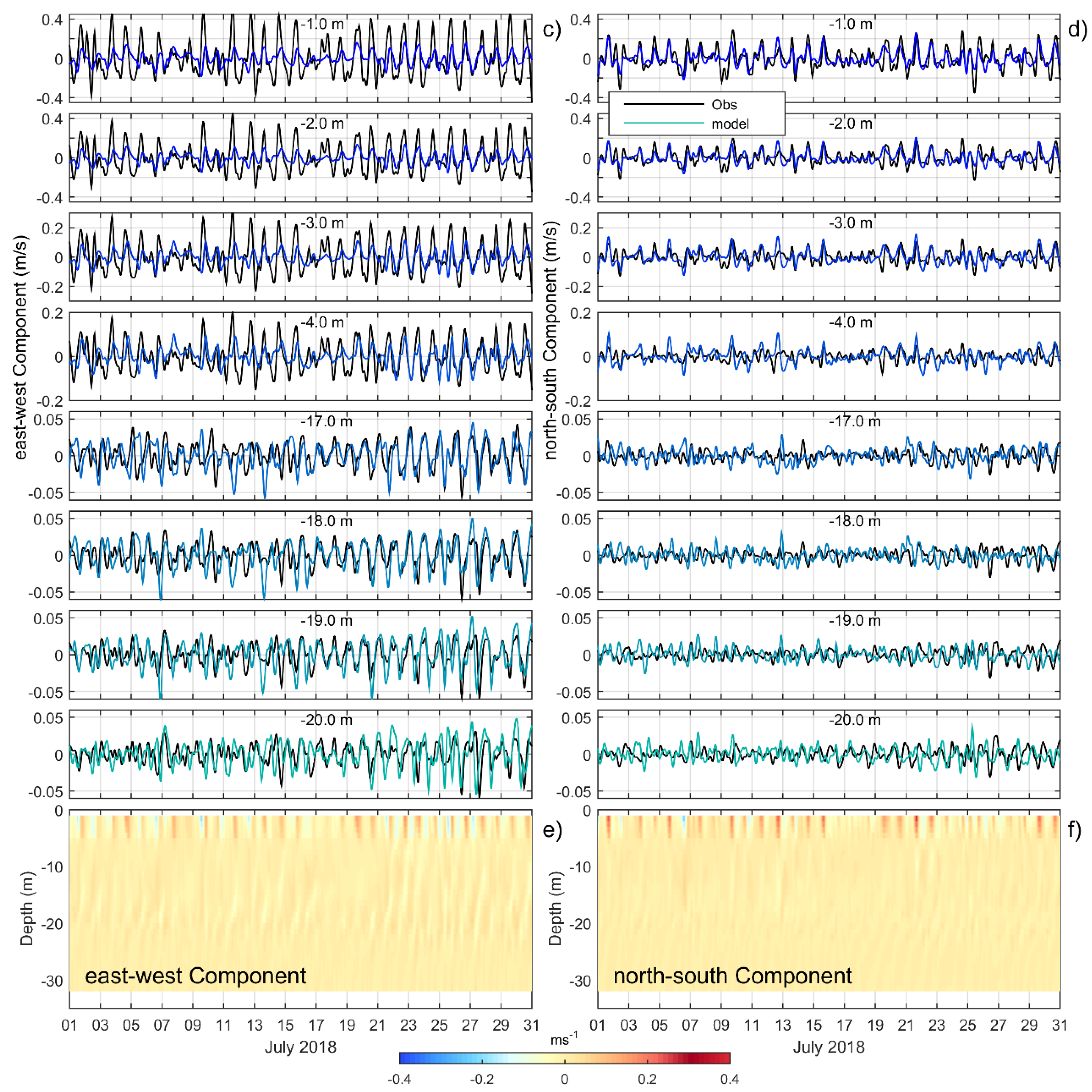
3.6. Current Meter
3.7. Numerical Model Results
3.7.1. Optimal Calibration
3.7.2. Model Validation
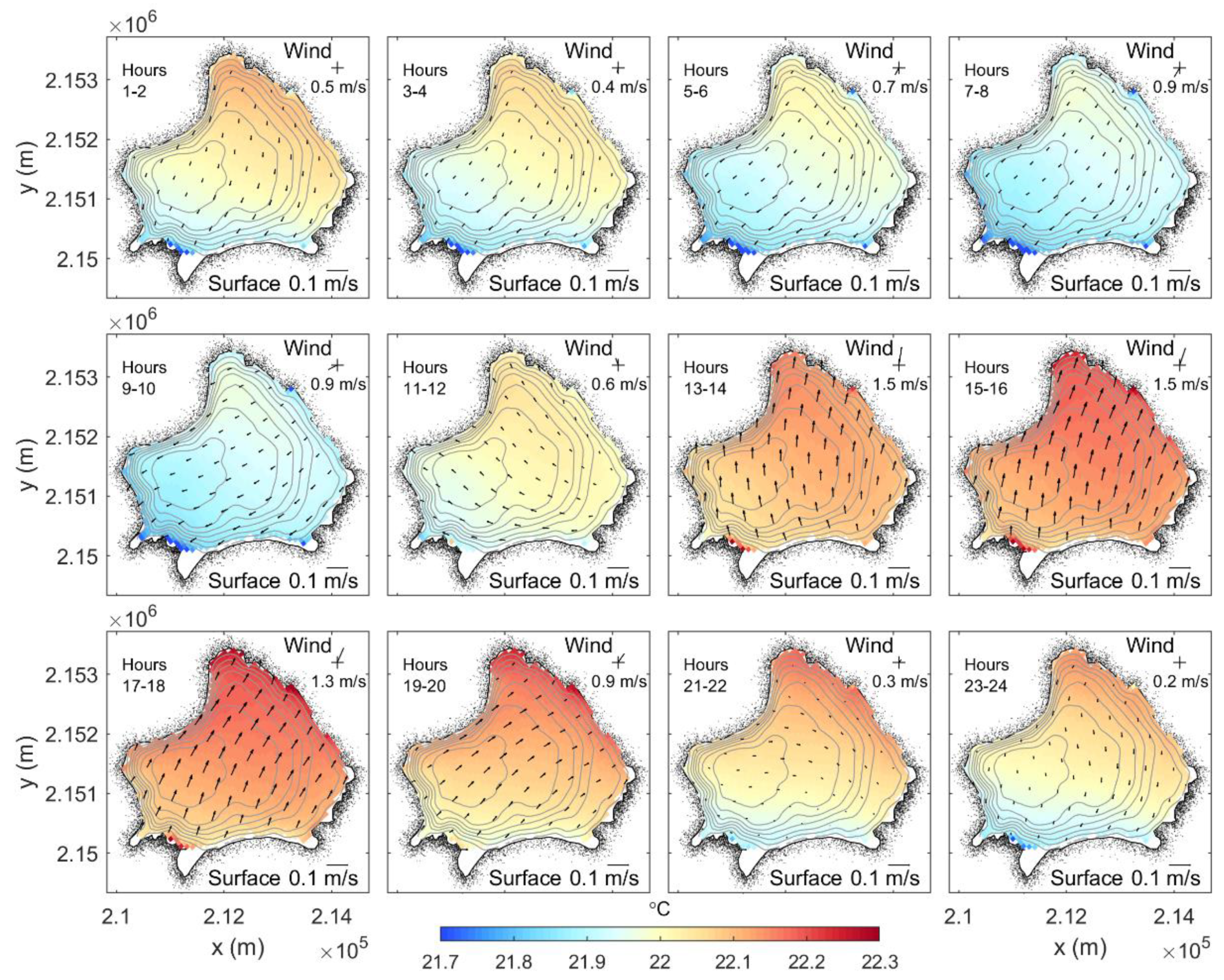
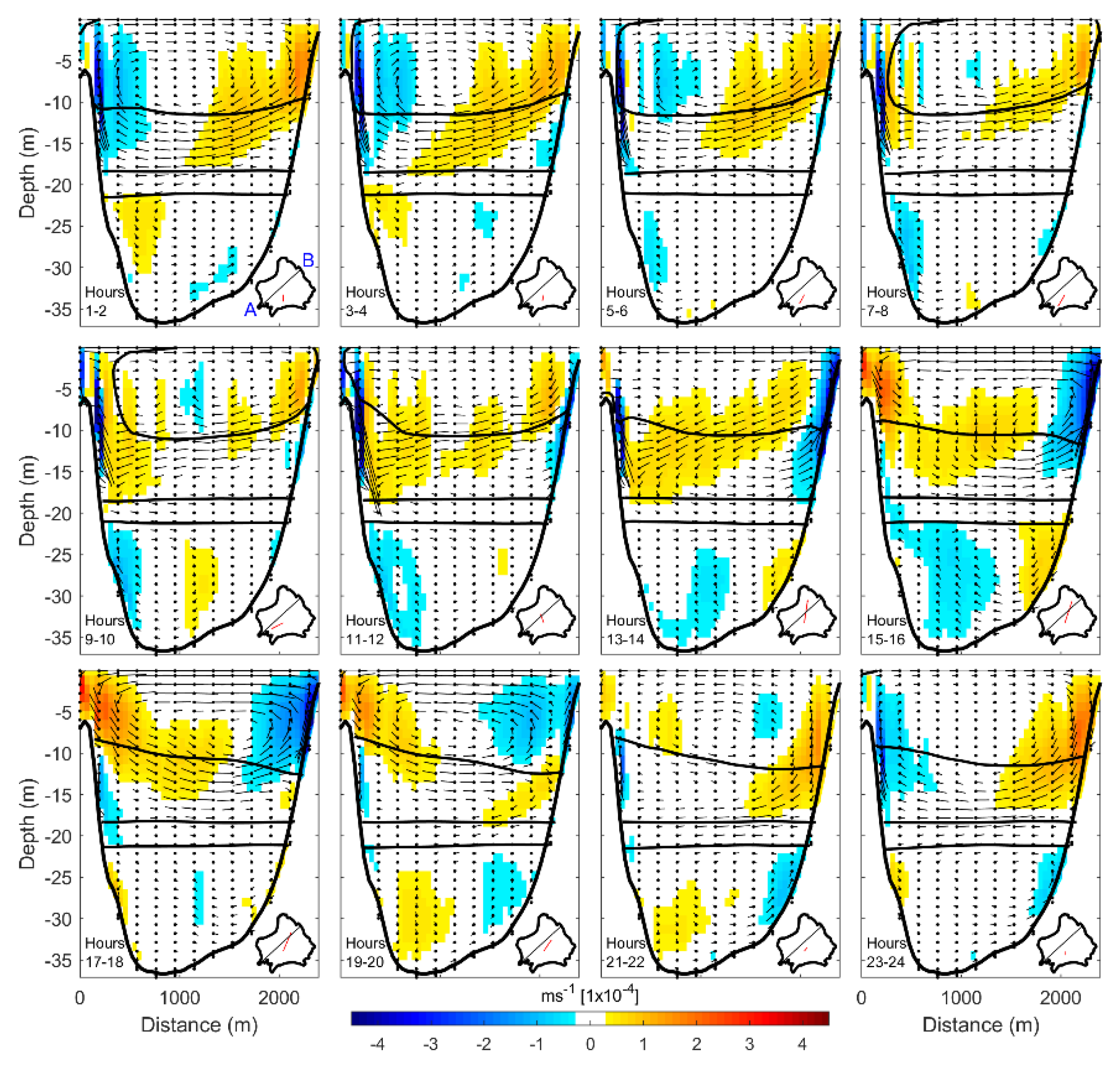
3.7.3. General Model Hydrography and Circulation
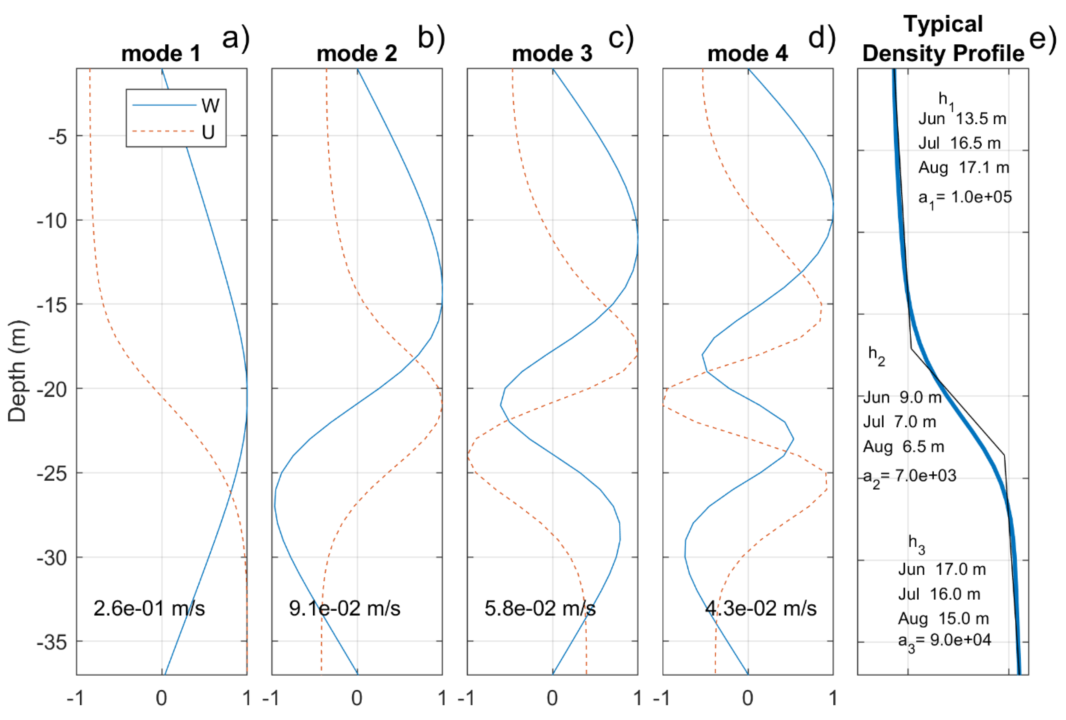
3.7.4. Normal Basin and Vertical Modes of Oscillation, Free and Forced Seiches
4. Conclusions
Author Contributions
Funding
Acknowledgments
Conflicts of Interest
References
- Koue, J.; Shimadera, H.; Matsuo, T.; Kondo, A. Evaluation of thermal stratification and flow field reproduced by a three-dimensional hydrodynamic model in Lake Biwa, Japan. Water 2018, 10, 47. [Google Scholar] [CrossRef]
- WWAP (United Nations World Water Assessment Programme). The United Nations World Water Development Report 2018: Nature-Based Solutions; UNESCO: Paris, France, 2018. [Google Scholar]
- Alcocer, J.; Bernal-Brooks, F.W. Limnology in Mexico. Hydrobiologia 2010, 644, 1–54. [Google Scholar] [CrossRef]
- Bernal-Brooks, F.W.; Dávalos-Lind, L.; Lind, O.T. Assessing trophic state of an endorheic tropical lake: The algal growth potential and limiting nutrients. Archiv für Hydrobiol. 2002, 153, 323–338. [Google Scholar] [CrossRef]
- Bernal-Brooks, F.W.; Sanchez Chavez, J.J.; Bravo Inclan, L.; Hernandez Morales, R.; Martinez Cano, A.K.; Lind, O.T.; Davalos-Lind, L. The algal growth-limiting nutrient of lakes located at Mexico’s Mesa Central. J. Limnol. 2016, 75, 169–178. [Google Scholar] [CrossRef]
- Antonopoulos, V.Z.; Gianniou, S.K. Simulation of water temperature and dissolved oxygen distribution in Lake Vegoritis. Greece. Ecol. Model. 2003, 160, 39–53. [Google Scholar] [CrossRef]
- Adrian, R.; O’Reilly, C.M.; Zagarese, H.; Baines, S.B.; Hessen, D.O.; Keller, W.; Weyhenmeyer, G.A. Lakes as sentinels of climate change. Limnol. Oceanogr. 2009, 54, 2283–2297. [Google Scholar] [CrossRef] [PubMed]
- Williamson, C.E.; Saros, J.E.; Vincent, W.F.; Smol, J.P. Lakes and reservoirs as sentinels, integrators, and regulators of climate change. Limnol. Oceanogr. 2009, 54, 2273–2282. [Google Scholar] [CrossRef]
- Chao, X.; Jia, Y.; Shields, F.D., Jr.; Wang, S.S.; Cooper, C.M. Three-dimensional numerical simulation of water quality and sediment-associated processes with application to a Mississippi Delta lake. J. Environ. Manag. 2010, 91, 1456–1466. [Google Scholar] [CrossRef] [PubMed]
- Mao, J.; Jiang, D.; Dai, H. Spatial–temporal hydrodynamic and algal bloom modelling analysis of a reservoir tributary embayment. J. Hydro Environ. Res. 2015, 9, 200–215. [Google Scholar] [CrossRef]
- Agarwal, A.; de los Angeles, M.S.; Bhatia, R.; Chéret, I.; Davila-Poblete, S.; Falkenmark, M.; Rees, J. Integrated water resources management. Glob. Water Partnersh. 2000, 29, 351–352. [Google Scholar]
- Kaçıkoç, M.; Beyhan, M. Hydrodynamic and water quality modeling of Lake Eğirdir. CLEAN–Soil Air Water 2014, 42, 1573–1582. [Google Scholar] [CrossRef]
- Cosgrove, W.J.; Loucks, D.P. Water management: Current and future challenges and research directions. Water Resour. Res. 2015, 51, 4823–4839. [Google Scholar] [CrossRef]
- Orlović, M.; Krajnović, A. Water management-an important challenge for modern economics. In DIEM: Dubrovnik International Economic Meeting; Sveučilište u Dubrovniku: Dubrovnik, Croatia, 2015; Volume 2, pp. 487–510. [Google Scholar]
- Soulignac, F.; Vinçon-Leite, B.; Lemaire, B.J.; Martins, J.R.S.; Bonhomme, C.; Dubois, P.; Tassin, B. Performance assessment of a 3D hydrodynamic model using high temporal resolution measurements in a shallow urban lake. Environ. Model. Assess. 2017, 22, 309–322. [Google Scholar] [CrossRef]
- Liu, L. Application of a Hydrodynamic and Water Quality Model for Inland Surface Water Systems. In Applications in Water Systems Management and Modeling; IntechOpen: Rijeka, Croatia, 2018. [Google Scholar] [CrossRef]
- Qin, B. Hydrodynamics of Lake Taihu, China. AMBIO 1999, 28, 669–673. [Google Scholar]
- Ji, Z.G. Hydrodynamics and Water Quality: Modeling Rivers, Lakes, and Estuaries; John Wiley and Sons: Hoboken, NJ, USA, 2008. [Google Scholar] [CrossRef]
- Chao, X.; Jia, Y.; Wang, S.S.; Hossain, A.A. Numerical modeling of surface flow and transport phenomena with applications to Lake Pontchartrain. Lake Res. Manag. 2012, 28, 31–45. [Google Scholar] [CrossRef]
- Zijlema, M. Computational Modelling of Flow and Transport. 2015. Available online: http://resolver.tudelft.nl/uuid:5e7dac47-0159-4af3-b1d8-32d37d2a8406 (accessed on 12 September 2018).
- Tsydenov, B.O.; Kay, A.; Starchenko, A.V. Numerical modeling of the spring thermal bar and pollutant transport in a large lake. Ocean Model. 2016, 104, 73–83. [Google Scholar] [CrossRef]
- Ndungu, J.N.; Chen, W.; Augustijn, D.C.; Hulscher, S.J. Analysis of the driving force of hydrodynamics in Lake Naivasha, Kenya. Open J. Mod. Hydrol. 2015, 5, 95. [Google Scholar] [CrossRef]
- Walters, R.A.; Carey, G.F.; Winter, D.F. Temperature computation for temperate lakes. Appl. Math. Model. 1978, 2, 41–48. [Google Scholar] [CrossRef]
- Imberger, J.; Patterson, J.C. Physical limnology. In Advances in Applied Mechanics; Academic Press Inc.: Cambridge, MA, USA; Elsevier Science: San Diego, CA, USA, 1990; Volume 27, pp. 303–475. [Google Scholar] [CrossRef]
- Imberger, J. Physical processes in lakes and oceans. In Coastal and Estuarine Studies; American Geophysical Union: Washington, DC, USA, 1998; Volume 54. [Google Scholar] [CrossRef]
- Hodges, B.R.; Imberger, J.; Saggio, A.; Winters, K.B. Modeling basin-scale internal waves in a stratified lake. Limnol. Oceanogr. 2000, 45, 1603–1620. [Google Scholar] [CrossRef]
- Hutter, K.; Chubarenko, I.P.; Wang, Y. Methods of Understanding Lakes as Components of the Geophysical Environment. In Physics of Lakes; Springer Science and Business Media: Berlin/Heidelberg, Germany, 2014; Volume 3. [Google Scholar] [CrossRef]
- Wahl, B.; Peeters, F. Effect of climatic changes on stratification and deep-water renewal in Lake Constance assessed by sensitivity studies with a 3D hydrodynamic model. Limnol. Oceanogr. 2014, 59, 1035–1052. [Google Scholar] [CrossRef]
- Morales-Marín, L.A.; French, J.R.; Burningham, H. Implementation of a 3D ocean model to understand upland lake wind-driven circulation. Environ. Fluid Mech. 2017, 17, 1255–1278. [Google Scholar] [CrossRef] [PubMed]
- Boehrer, B.; Schultze, M. Stratification of lakes. Rev. Geophys. 2008, 46. [Google Scholar] [CrossRef]
- Mortimer, C.H. Water movements in lakes during summer stratification; evidence from the distribution of temperature in Windermere. Philos. Trans. R. Soc. Lond. Ser. B Biol. Sci. 1952, 236, 355–398. [Google Scholar] [CrossRef]
- Martínez-Almeida, V.; Tavera, R. A hydrobiological study to interpret the presence of desmids in Lake Zirahuén, México. Limnologica 2005, 35, 61–69. [Google Scholar] [CrossRef][Green Version]
- Mendoza, R.; Silva, R.; Jiménez, A.; Rodríguez, K.; Sol, A. Lake Zirahuen, Michoacan, Mexico: An approach to sustainable water resource management based on the chemical and bacterial assessment of its water body. Sustain. Chem. Pharm. 2015, 2, 1–11. [Google Scholar] [CrossRef]
- Paniagua, C.F.O. Espejo de los Dioses: Estudios sobre Ambiente y Desarrollo en la Cuenca del Lago de Zirahuén; Universidad Michoacana de San Nicolás de Hidalgo: Morelia, Mexico, 2010. [Google Scholar]
- Ortega, B.; Vázquez, G.; Caballero, M.; Israde, I.; Lozano-García, S.; Schaaf, P.; Torres, E. Late Pleistocene: Holocene record of environmental changes in lake Zirahuen, Central Mexico. J. Paleolimnol. 2010, 44, 745–760. [Google Scholar] [CrossRef]
- Vázquez, G.; Ortega, B.; Davies, S.J.; Aston, B.J. Registro sedimentario de los últimos ca. 17000 años del lago de Zirahuén, Michoacán, México. Bol. Soc. Geol. Mex. 2010, 62, 325–343. [Google Scholar]
- Deltares. Simulation of Multi-Dimensional Hydrodynamic Flows and Transport Phenomena, Including Sediments; User Manual Delft3D-FLOW; Version 3.15; Deltares: Delft, The Netherlands, 2020. [Google Scholar]
- Lesser, G.; Roelvink, D.; Van Kester, J.; Stelling, G. Development and validation of a three-dimensional morphological model. Coast. Eng. 2004, 51, 883–915. [Google Scholar] [CrossRef]
- Jorgensen, S.E.; Loffler, H.; Rast, W.; Straskraba, M. Lake and Reservoir Management; Elsevier Science: Amsterdam, The Netherlands, 2005; Volume 54. [Google Scholar]
- Jones, H.F.E.; Hamilton, D.P. Hydrodynamic Modelling of Lake Whangape and Lake Waahi; Waikato Technical Report. 2014. Available online: https://www.waikatoregion.govt.nz/assets/WRC/WRC-2019/TR201424.pdf (accessed on 7 May 2019).
- Dissanayake, P.; Hofmann, H.; Peeters, F. Comparison of results from two 3D hydrodynamic models with field data: Internal seiches and horizontal currents. Inland Waters 2019, 9, 239–260. [Google Scholar] [CrossRef]
- Launder, B.E.; Spalding, D.B. The numerical computation of turbulent flows. In Numerical Prediction of Flow, Heat Transfer, Turbulence and Combustion; Elsevier: Amsterdam, The Netherlands, 1983; pp. 96–116. [Google Scholar] [CrossRef]
- Chavent, G. Nonlinear Least Squares for Inverse Problems: Theoretical Foundations and Step-by-Step Guide for Applications; Springer: Dordrecht, The Netherlands, 2010. [Google Scholar] [CrossRef]
- Coleman, T.F.; Li, Y. On the Convergence of reflective newton methods for large-scale nonlinear minimization subject to bounds. Math. Program. 1994, 67, 189–224. [Google Scholar] [CrossRef]
- Byrd, R.H.; Schnabel, R.B.; Shultz, G.A. Approximate solution of the trust region problem by minimization over two-dimensional subspaces. Math. Program. 1988, 40, 247–263. [Google Scholar] [CrossRef]
- Thomson, R.E.; Emery, W.J. Data Analysis Methods in Physical Oceanography; Elsevier: Amsterdam, The Netherlands, 2014. [Google Scholar] [CrossRef]
- Taylor, K.E. Summarizing multiple aspects of model performance in a single diagram. J. Geophys. Res. Atmos. 2001, 106, 7183–7192. [Google Scholar] [CrossRef]
- Heaps, N.S. Seiches in a narrow lake, uniformly stratified in three layers. Geophys. J. Int. 1961, 5, 134–156. [Google Scholar] [CrossRef]
- LaZerte, B.D. The dominating higher order vertical modes of the internal seiche in a small lake. Limnol. Oceanogr. 1980, 25, 846–854. [Google Scholar] [CrossRef]
- Zhou, X.-M.; Tang, B.-H.; Wu, H.; Li, Z.-L. Estimating net surface longwave radiation from net surface shortwave radiation for cloudy skies. Int. J. Remote Sens. 2013, 34, 8104–8117. [Google Scholar] [CrossRef]


| Weather Station | CTD | Thermistor Chain | Water Level | Acoustic Current Meter Profiler (ADP) | |
|---|---|---|---|---|---|
| February |  | ||||
| March |  | ||||
| April |  | ● | |||
| May |  |  | ● |  | |
| June |  | ● |  |  | |
| July |  | ||||
| September | ● |  | |||
| November |  |  |
| Temperature | Horizontal Velocity | ||||||
|---|---|---|---|---|---|---|---|
| Depth (m) | RMSE (°C) | R2 | Depth (m) | RMSE | R2 | ||
| U (m/s) | V (m/s) | U | V | ||||
| 13 | 0.37 | 0.84 | 1 | 0.2 | 0.1 | 0.22 | 0.48 |
| 15 | 0.61 | 0.42 | 2 | 0.1 | 0.1 | 0.18 | 0.38 |
| 18 | 0.82 | 0.10 | 3 | 0.1 | 0.04 | 0.15 | 0.27 |
| 20 | 0.47 | 0.08 | 4 | 0.1 | 0.02 | 0.14 | 0.12 |
| 23 | 0.43 | 0.07 | 17 | 0.02 | 0.01 | 0.18 | 0.02 |
| 25 | 0.33 | 0.05 | 18 | 0.02 | 0.01 | 0.26 | 0.01 |
| 28 | 0.12 | 0.03 | 19 | 0.02 | 0.01 | 0.22 | 0.01 |
| 30 | 0.08 | 0.02 | 20 | 0.02 | 0.01 | 0.10 | 0.01 |
| Basin Modes Seiches | |||||
| External Mode [min] | Internal Modes [h] | ||||
| Mode-1 | Mode-2 | Mode-3 | Mode-4 | ||
| Numerical Model with Flat Bottom at 40 m (Tn~T1/n, n > 1) | |||||
| n = 1 | n = 2 | n = 3 | n = 4 | ||
| 6.7 | T1 = 7.9 | 4.0 | 2.7 | 2.1 | |
| Numerical Model with Real Bathymetry | |||||
| 7.4 | T1 = 5.9 | 3.0 | 2.0 | 1.4 | |
| Vertical Modes | |||||
| Three Layers Model Continuous Density | |||||
| V Mode 1 | V Mode 2 | V Mode 3 | V Mode 4 | ||
| June | 6.8 | 6.6/n | 21.1/n | 35.6/n | 43.3/n |
| July | 6.8 | 7.2/n | 25.2/n | 39.1/n | 44.4/n |
| August | 6.9 | 7.6/n | 26.7/n | 40.0/n | 45.9/n |
| Numerical Integration with N (z) | |||||
| June | 7.0/n | 20.9/n | 33.9/n | 46.2/n | |
| July | 7.7/n | 23.2/n | 36.8/n | 49.2/n | |
| Augyst | 8.0/n | 22.3/n | 35.2/n | 47.4/n | |
© 2020 by the authors. Licensee MDPI, Basel, Switzerland. This article is an open access article distributed under the terms and conditions of the Creative Commons Attribution (CC BY) license (http://creativecommons.org/licenses/by/4.0/).
Share and Cite
Gasca-Ortiz, T.; Pantoja, D.A.; Filonov, A.; Domínguez-Mota, F.; Alcocer, J. Numerical and Observational Analysis of the Hydro-Dynamical Variability in a Small Lake: The Case of Lake Zirahuén, México. Water 2020, 12, 1658. https://doi.org/10.3390/w12061658
Gasca-Ortiz T, Pantoja DA, Filonov A, Domínguez-Mota F, Alcocer J. Numerical and Observational Analysis of the Hydro-Dynamical Variability in a Small Lake: The Case of Lake Zirahuén, México. Water. 2020; 12(6):1658. https://doi.org/10.3390/w12061658
Chicago/Turabian StyleGasca-Ortiz, Tzitlali, Diego A. Pantoja, Anatoliy Filonov, Francisco Domínguez-Mota, and Javier Alcocer. 2020. "Numerical and Observational Analysis of the Hydro-Dynamical Variability in a Small Lake: The Case of Lake Zirahuén, México" Water 12, no. 6: 1658. https://doi.org/10.3390/w12061658
APA StyleGasca-Ortiz, T., Pantoja, D. A., Filonov, A., Domínguez-Mota, F., & Alcocer, J. (2020). Numerical and Observational Analysis of the Hydro-Dynamical Variability in a Small Lake: The Case of Lake Zirahuén, México. Water, 12(6), 1658. https://doi.org/10.3390/w12061658