Understanding the Role of Shallow Groundwater in Improving Field Water Productivity in Arid Areas


1
Water Conservancy and Civil Engineering College, Inner Mongolia Agricultural University, Saihan District, Hohhot 010018, China
2
Centre for Agricultural Water Research in China, China Agricultural University, Beijing 100083, China
3
Institute of Water Resources for Pastoral Area, China Institute of Water Resources and Hydropower Research, Hohhot 010020, China
*
Author to whom correspondence should be addressed.
Water 2020, 12(12), 3519; https://doi.org/10.3390/w12123519
Submission received: 8 November 2020
/
Revised: 9 December 2020
/
Accepted: 9 December 2020
/
Published: 15 December 2020
(This article belongs to the Section Water Use and Scarcity)
Abstract
:Soil water and salt transport in soil profiles and capillary rise from shallow groundwater are significant seasonal responses that help determine irrigation schedules and agricultural development in arid areas. In this study the Agricultural Water Productivity Model for Shallow Groundwater (AWPM-SG) was modified by adding a soil salinity simulation to precisely describe the soil water and salt cycle, calculating capillary fluxes from shallow groundwater using readily available data, and simulating the effect of soil salinity on crop growth. The model combines an analytical solution of upward flux from groundwater using the Environmental Policy Integrated Climate (EPIC) crop growth model. The modified AWPM-SG was calibrated and validated with a maize field experiment run in 2016 in which predicted soil moisture, soil salinity, groundwater depth, and leaf area index were in agreement with the observations. To investigate the response of the model, various scenarios with varying groundwater depth and groundwater salinity were run. The inhibition of groundwater salinity on crop yield was slightly less than that on crop water use, while the water consumption of maize with a groundwater depth of 1 m is 3% less than that of 2 m, and the yield of maize with groundwater depth of 1 m is only 1% less than that of 2 m, under the groundwater salinity of 2.0 g/L. At the same groundwater depth, the higher the salinity, the greater the corn water productivity, and the smaller the corn irrigation water productivity. Consequently, using modified AWPM-SG in irrigation scheduling will be beneficial to save more water in areas with shallow groundwater.
1. Introduction
In many semi-arid and arid regions of the world, irrigated agriculture consumes most of the available water. For example, in China, agricultural water use accounts for 60% of the total water use and 90% of the agricultural water is used for irrigation [1,2]. Therefore, developing water-saving agriculture and enhancing water productivity are of great significance for ensuring water security, food security, and ecological security in China [3].
In particular, in the Hetao irrigation district, which is a typical arid area with shallow groundwater and affected by soil salinization, various water-saving measures including lining of main, sub-main and distributor canals have been implemented since 2000 [4,5]. The application of water saving measures has led to a decline in the groundwater table that controls the waterlogging and salinity. Soil salinization is a serious environmental problem [6,7,8]. Healthy soils and healthy land are the basic conditions for the successful implementation and realization of the sustainable development goals related to food, healthy water and climate [9,10,11,12,13]. Therefore, understanding water and salt balance under shallow groundwater is significant for sustainable agriculture.
In districts with shallow groundwater, such as the Hetao Irrigation district, capillary rise from groundwater can be used to supplement surface water irrigation and in closed basins, it can possibly save water for irrigating additional areas. At the same time, the soil acts a filter for groundwater [14]. Then capillary rise from groundwater depends on several factors such as groundwater table depth, soil hydraulic properties, crop growth stage, weather and irrigation [15,16]. According to the entropy model, land-use, soil order and rainfall factors had the highest impact on groundwater potential [17]. Several studies have quantified the amount of water derived from groundwater and found that 20%–40% of the evapotranspiration can be met by capillary rise from water tables at depths of 0.70–1.50 m [18,19,20,21,22,23,24]. With lysmeter experiments, Kahlown and Ashraf [25] found that under the water table at 0.5 m depth, wheat met its entire water requirement from the groundwater and the sunflower’s required water absorbed from groundwater is greater than 80%.
Soil salinity is a limiting factor for crop growth, especially within shallow groundwater. Pan et al. used a Soil Water Atmosphere Plant (SWAP) model to simulate soil water-salt balance, summer maize yield and water use efficiency under different irrigation schedules [26]. A modified HYDRUS model was used in simulating polyfluoroalkyl substances (PFAS) transport in the vadose zone [27]. By analysing satellite-based remote sensing images, Yu et al. [8] indicated that groundwater depth was the major controlling factor for regional soil salinity. Metternicht et al. [28] adopted remote sensing to analyze the spatial distribution and temporal changes in soil salinity.
Yield, water productivity (WP), and irrigation water productivity (IWP) vary with both groundwater depth and soil salinity. Mejia et al. [29] conducted a two-year study to investigate the effect of the groundwater table on the corn yield and found a 5%–10% greater yield for corn, and 23% for soybeans at 0.5–0.75 m groundwater depth compared with the same treatment with groundwater depth more than 1 m. Wang et al. [30] investigated the water and salt transport features for saline soil through drip irrigation under film, and found that the increase in irrigation water would expand the standard district for the normal growth of plants. Huo et al. [31] reported that irrigation water productivity (IWP) increased with shallower groundwater tables.
Although experimental results have indicated that shallow groundwater can contribute to crop water use, it is seldom used in irrigation scheduling because measuring the capillary upward flux is complex and cannot be performed routinely. Therefore, models are the only way to obtain fluxes. However, most of the irrigation management models assume that the groundwater is sufficiently deep that the water percolates downwards out of the plant roots [32,33,34]. Several methods that can estimate the upward water such as Hydrus and SWAP are cumbersome because they require spatially varying input data such as the soil water retention curve and unsaturated hydraulic conductivity that are not easily available [35]. Prathapar and Qureshi [36] used the SWAP model to evaluate consequences of deficit irrigation in semi-arid areas with a shallow water table in Pakistan. Other models, such as by Healy and Cook [37] and Ayars et al. [38] are based on measured moisture content or water-table fluctuations and cannot be used in routine applications. Additionally, common numerical methods require a lot of verification and depend on soil parameters.
Because of the intensive data requirements of the above-mentioned models for use in irrigation management with shallow groundwater, the AWPM-SG was established in previous studies to simulate the water cycle in shallow groundwater areas. The objective of this study is, therefore, to (1) develop a modified model that couples soil water and salt and crop growth to analyze the field water and salt cycle and groundwater contribution to crop evapotranspiration; and (2) investigate the effect of groundwater depth and groundwater salinity on yield, crop evapotranspiration, water productivity and irrigation water productivity of maize. Without affecting the maize yield, the irrigation water can be reduced within a reasonable range.
2. Materials and Methods
2.1. Experiments
For model calibration and validation, field experiments by Wang in 2016 in Fenzidi located in the Hetao irrigation district were used. The experimental station was located in an open field and had a representative climate, soil, and groundwater conditions.
The Hetao irrigation district, is located in the western part of the Inner Mongolia Autonomous Region. The study site has a typically arid and semi-arid continental climate. The average annual rainfall is 142 mm and falls mainly from June to August. The average annual pan evaporation is 2300 mm. The average number of sunlight hours per month is 266 h. The mean annual temperature is 7 ℃, with monthly averages of −10.1 in January to 23.8 ℃ in July (Figure A1 in the Appendix B). Soils begin to freeze in the second half of November to a maximum depth of approximately 1.0–1.3 m, and is completely thawed by the middle of May. Groundwater depth varies between 1.2 and 3.8 m.
The experiment growing maize was carried out by Wang in 2016 [39]. The maize (Kehe-8) commonly grown in Hetao was planted in late April and harvested in late September. Cultivation practices were similar to the practices of farmers and recommended by extension agents. Three times during the growing season 216 and 218 mm of water were applied for the field plots named F1 and F2 (Table 1). The irrigation amount refers to the local farmers’ field. Nitrogen fertilizers were applied at a rate of 207 kg/ha for the first irrigation, and 103 kg/ha for the third irrigation in 2016.
During the growing period, the meteorological data, including air temperature, sunshine hours, relative humidity and wind speed were taken from micrometeorological stations in farmland and were used to calculate the FAO (Food and Agricultural Organization of the United Nations) Penman-Monteith reference evapotranspiration (ET0). Daily rainfall was measured using a rain gauge at the experimental site. The rainfall was 55.1 mm, with more than 70% of precipitation occurring in July and August. The main weather data are shown in Figure A1 in the Appendix B.
The particle size distribution was obtained using a laser particle analyzer. The main physical properties of the soil are shown in Table 2. In the root zone, the soil is silty loam, which is the representative soil texture in this region. The dry bulk density was obtained by oven drying undisturbed soil samples of 100 cm3 at 105 °C for 48 h. Saturated hydraulic conductivity was estimated in eight 100 cm3 undisturbed soil samples using a constant-head permeameter [40]. Soil water retention curves were determined for each horizon in 100 cm3 undisturbed soil samples using a pressure membrane apparatus (SEC-1000, Soilmoisture Equipment Corporation, CA, US). The fitted soil hydraulic parameters of the Muchlem-van Genuchten model are presented in Table 3.
2.2. Data
The soil moisture content was measured every day using an Automatic Soil Moisture Monitor (Hydra Probe, Stevens Water Monitoring Systems, Inc., Portland, Oregon, USA). The soil moisture was measured at 20 cm intervals from the surface to a depth of 100 cm. At the same time, it was calibrated with drying method through earth-fetching at regular times.
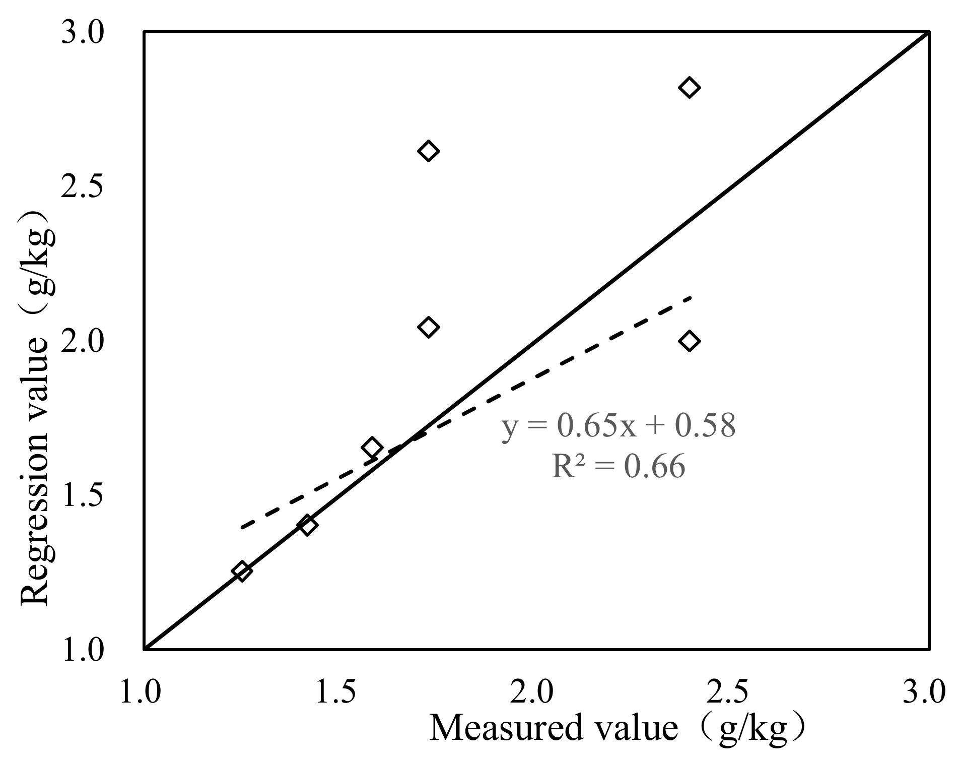
Soil salinity was measured similarly to the soil water content. It was also measured every day using an automatic soil moisture monitor (Hydra Probe) at 20 cm intervals. Because the soil electrical conductivity (EC) monitored by Hydra Probe was affected by soil water and soil salinity, the soil electrical conductivity is directly related with soil water content. Two references that used Hydra Probe showed the results. In the study of Valdes et al., soil bulk EC (ECb) monitored by Hydra Probe is a function of both water and pore water EC (ECp). Then firstly we transfer the ECb to ECp based on soil water content [41]. Leao et al. reported that soil apparent bulk electrical conductivity is a function of soil water content, pore solution electrical conductivity and solid phase electrical conductivity [42]. We assumed the soil salinity is a function of soil water and soil electrical conductivity monitored by Hydra Probe. Because the monitored soil electrical conductivity needed to be modified according to the soil salinity obtained by earth-fetching, we take the regression as follows:
where S is the soil total salinity (g/kg), EC is the soil electrical conductivity monitored by Hydra Probe (ms/cm), and SWC is soil water content (cm3/cm3). Figure A2 in the Appendix B shows the contrast between the regression value and measured value.
The groundwater depth was monitored daily during the crop growth period by monitoring the piezo metric head of the probe (Hobe 20).
The crop leaf area index (LAI) was measured every 6–12 days using a leaf area metre (YMJ-B).
Dry maize yield was determined after harvesting.
2.3. Model Description
2.3.1. Modified Agricultural Water Productivity Model for Shallow Groundwater
In this study, considering the high soil salinity in the Hetao irrigation area, the developed Agricultural Water Productivity Model for Shallow Groundwater (AWPM-SG) model was modified to simulate the actual soil water, soil salinity and groundwater depth. The developed AWPM-SG is the coupling of a crop growth Environmental Policy Integrated Climate (EPIC) model and a soil moisture model of the Watershed Irrigation Potential Estimation (WIPE) root and vadose zone that simulates both upward movement from groundwater and percolation to the groundwater. This was originally developed by Saleh et al. for investigating the impact of irrigation management schemes on groundwater levels in Bangladesh [43,44]. The structure of the modified AWPM-SG is shown in Figure 1. The model simulates water and salt flux on daily time steps and require few parameters (soil hydraulic parameters and crop growing parameters), which are listed in Table 3 and Table 4 and. The three parts of the modified AWPM-SG consist of a crop module, an actual evapotranspiration module and a soil module, which are coupled for the first time in the AWPM-SG [15] (Figure A3 drawn by Xiaoyu Gao in the Appendix B). This modified model mainly considers soil salt transport and its effect on crop growth, especially in the shallow groundwater district (Method in Appendix A). The modified model is described in detail in the Appendix A. An overview of modified AWPM-SG is given below.
2.3.2. Crop Module Considering Soil Salinity
The crop module of AWPM-SG is mainly based on the Environmental Policy Integrated Climate (EPIC) model. It has been tested and applied widely around the world. Currently the EPIC model has evolved into a comprehensive model capable of simulating photosynthesis, evapotranspiration and other major plant and soil process [45]. The crop module includes the phonological development, crop growth indexes (LAI, biomass, root growing, crop yield) and water productivity (WP, IWP).
2.3.3. Description of Soil Module Considering Soil Salinity
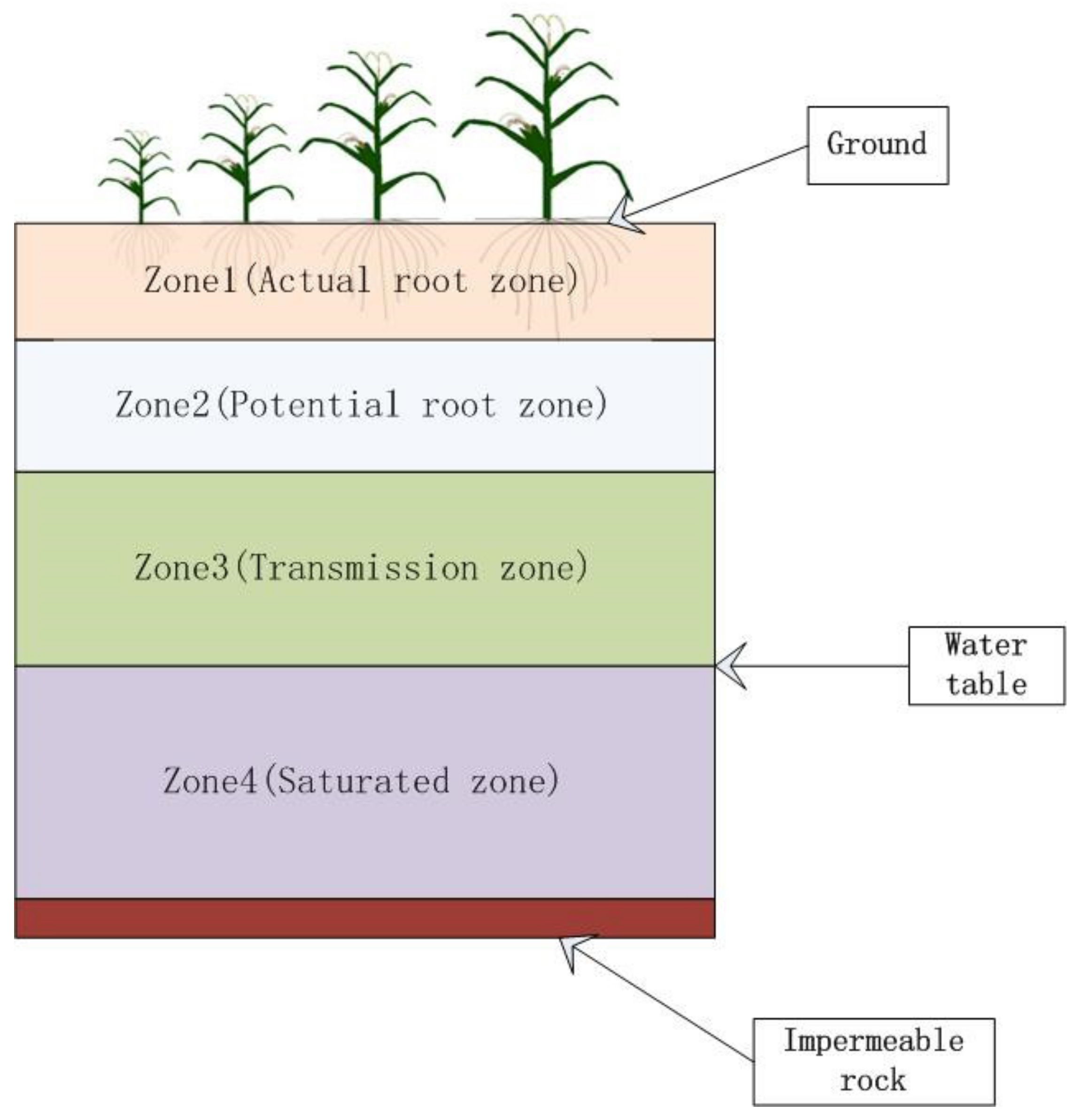
Because EPIC cannot simulate the crop growth above the ground without the soil data, EPIC was coupled with the modified watershed irrigation potential estimation model (WIPE) to simulate the whole water recycle. The WIPE model was designed by Saleh et al. [44] to study the impact of irrigation management schemes on groundwater levels in Bangladesh. The model divides the soil profile into four zones namely the actual root zone, potential root zone, transmission zone, and the saturated zone as shown in Figure A3 in the Appendix B. The soil texture in zone 1 and 2 are same. The zone 1 is calculated using the water and salt balance method. The WIPE model simulates both downward recharge when the soil moisture in zone 2 is greater than field capacity and upward movement when the soil moisture is below field capacity using an analytical solution developed by Gardner [46]. This is a one-dimensional model employing the Thornthwaite-Mather procedure to calculate the recharge below the root zone to the aquifer and is primarily applicable to shallow aquifers. Full details of the model are provided in Appendix A (modified Agricultural Water Productivity Model for Shallow Groundwater).
2.3.4. Actual Evapotranspiration Module Considering Soil Salinity
Actual evapotranspiration is an input to the EPIC model. We used the model of Kendy et al. that previously was able to calculate the actual evapotranspiration from soil-water and salt storage in North China Plain with good accuracy [33]. In this model, the ratio of Ep to Tp depends upon the development stage of the leaf canopy, moisture content, soil salinity and root development. The input data are the daily leaf area index, LAI simulated by the EPIC model and simulated soil moisture and soil salinity of actual root zone (zone 1) by WIPE model and water balance.
2.4. Model Calibration and Validation
The simulation period for maize lasted from late April to late September in 2016 using the observed initial soil water content and groundwater depth subject to the imposed irrigation schedule and fertilizer applications. The S1 data were used for calibration and S2 to validate the model. Soil moisture and soil salinity in the top 90 cm (zones 1 and 2), groundwater depth, and LAI were simulated. The soil hydraulic parameters (md, ms, C, α and ks) and the crop parameters were calibrated (Table 3 and Table 4). During the calibration, we set the parameters of the model according to the measured data and recommended values. We then analyzed both their sensitivity and uncertainty of parameters and found the sensitive parameters for soil water, groundwater depth and crop LAI, such as maximum leaf area index (LAImx), mf and so on. Then we adjusted the parameters as their sensitivity to make the simulation result of the model closer to the measured data. Finally, the calibrated parameters were used to validate the model using the S2 data. The default values of the EPIC model for maize were used as initial values for simulating crop growth [47]. The default value of the maximum rooting depth was 90 cm, as measured in the experiment by Wang [39]. Initial soil water content and groundwater depth were specified according to the measurements. A sensitivity and uncertainty analysis of parameters was performed once more for soil water content, soil salinity, groundwater depth and crop LAI.
The upper boundary condition was determined by the actual evaporation and transpiration rates, and the irrigation and precipitation were fluxed. A no-flux boundary condition was specified at the bottom of the column.
The mean relative error (MRE), root mean square error (RMSE), Nash and Sutcliffe model efficiency (NSE), coefficient of determination (R2) and coefficient of regression (b) were used to quantify the model-fitting performance for both calibration and validation processes [48]. A MRE close to 0 indicates good model predictions. A RMSE value close to 0 indicates good model predictions. NSE = 1.0 represents a perfect fit, NSEclose to 0 represents the predicted values near the averaged measurement, and negative NSEvalues indicate that the mean observed value is a better predictor than the simulated value. An R2 value close to 1 indicates good model predictions. A b value close to 1 indicates good model predictions [49].
2.4.1. Sensitivity Analysis of Parameters
By increasing or decreasing the percentage of the parameters, the variation of ET, groundwater depth, LAI, soil water and soil salinity were analyzed at 90 cm. Then the sensitivity of each parameter on ET, groundwater depth, LAI and soil water and salinity of 90 cm can be obtained (Figure A4).
2.4.2. Uncertainty Analysis of Parameters
The d-factor was used to analyze the uncertainty of the parameters [50,51]. The d-factor is indicative of the average distance between the upper and lower confidence intervals (in this study the 95% prediction interval). The d-factor was calculated as follows:
where dx is the average distance between the lower XL and upper limits of the confidence interval and σx is the standard deviation of the observed data. n is the number of data points. Larger d-factors lead to larger uncertainty.
2.5. Scenarios for Evaluation of Water Use and Yield
After calibration and validation of the modified AWPM-SG, the model was used to determine the response of groundwater depth (GWD) and groundwater salinity on water use, maize yield, WP and IWP. To do so the modified AWPM-SG was run for ten scenarios with 7 GWD levels (100, 150, 200, 250, 300, 350 and 400 cm) and 3 groundwater salinity levels (S, S1, S2-groundwater salinity of 1 g/L, 2 g/Land 4 g/L) were simulated. The rainfall and irrigation schedule for the simulation treatment was similar to that in the F1 plot used for calibration of the model. The initial soil water, groundwater depth soil texture and fertilizer application are set as the data of F1 plot. The meteorology data was based on the data in 2016.
The response of groundwater depth (GWD) and groundwater salinity on water use, maize yield, WP and IWP were investigated through running model with MATLAB. And then regression between WP, IWP and groundwater depth under different groundwater salinity was carried out using Origin 2017.
3. Results
3.1. Evaluation of the Modified AWPM-SG
Data from the experimental study conducted in 2016 at S1 and S2 sites of the Fenzidi experimental station in the Hetao irrigation district, were used to calibrate and validate the modified AWPM-SG. The maize (Kehe-8) commonly grown in the Hetao irrigation district was planted in late April and harvested in late September. Experiments were carried out in two replicates.
The experimental data of F1 were used for calibration and F2 for validation. The soil data and crop data input are shown in Table 3 and Table 4. The accuracy of the fit test is shown in Table 5. In the case where the observed data at F1 and F2 sites was remained nearly the same as the simulated values, while the data of validation treatment at F2 sites gave unrealistic results, which was due to the abnormal growth of crops at the F2 site.
3.1.1. Soil Moisture: Calibration and Validation
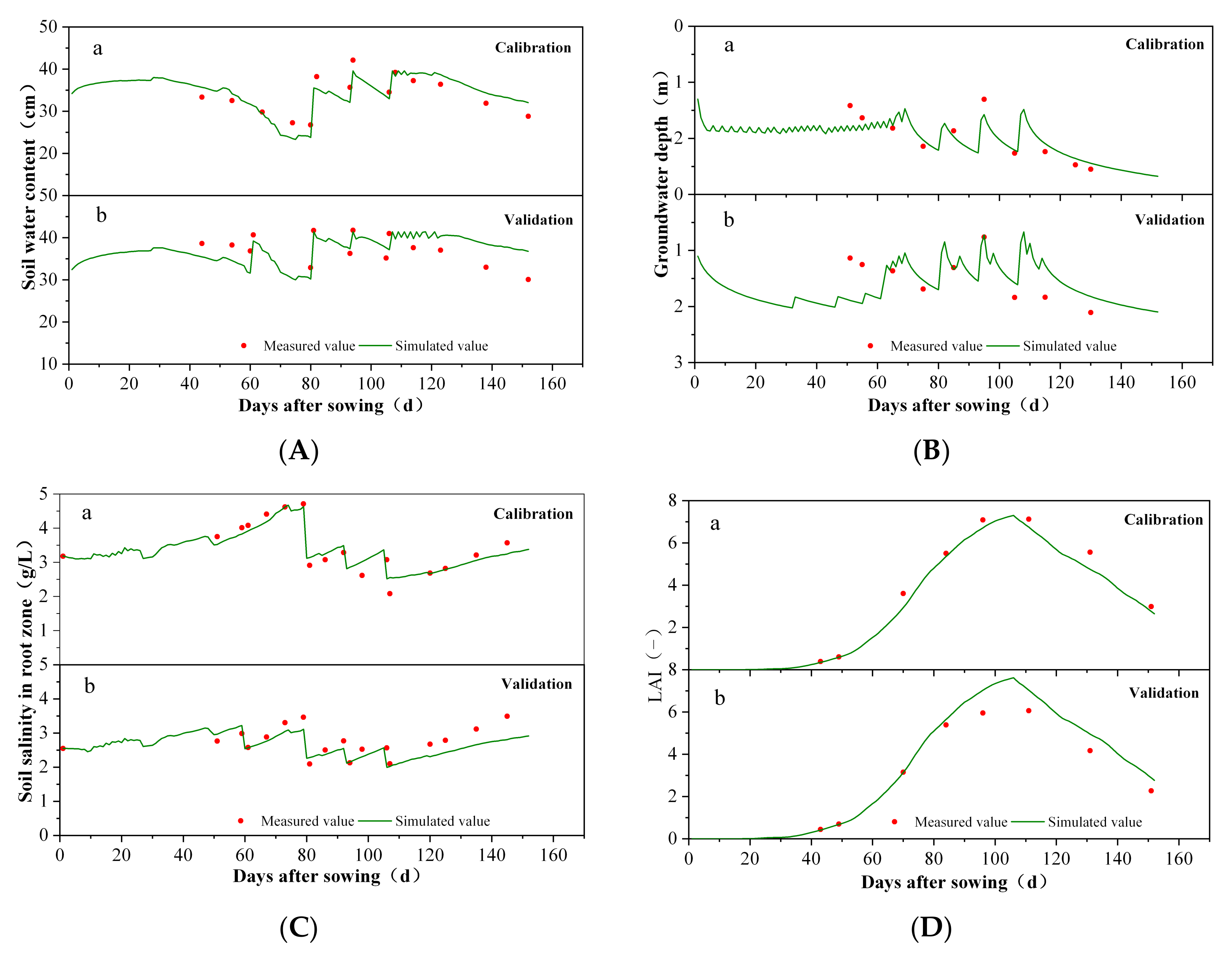
The soil water content of the top 90 cm (zones 1 and 2) was used to calibrate and validate the model. Simulated mean soil water content at the F1 site in the 90 cm soil zone was generally satisfactorily simulated with a mean relative error (MRE) and Nash and Sutcliffe model efficiency (NSE) of −1.07% and 0.49, respectively (Figure 2A). The accuracy of fit was reasonable for most statistics presented in Table 5. At the S2 site the soil moisture was well predicted with the calibrated input data (Figure 2A, Table 5) including an NSE of 0.28 and R2 of 1 (Table 5). For calibration and validation, the averaged RMSE value was 2.11 cm.
3.1.2. Soil Salinity: Calibration and Validation
The soil salinity of the top 90 cm (zones 1 and 2) was used to calibrate and validate the model. Simulated mean soil salinity at the F1 site in the 90 cm soil zone was generally satisfactorily simulated with the MRE and NSE of −2.57% and 0.85 (Figure 2B). The goodness of fit was reasonable for most statistics presented in Table 5. At the S2 site, the soil salinity was well predicted with the calibrated input data (Figure 2A, Table 5), including an NSE of 0.17 and b of 0.92 (Table 5). For calibration and validation, the averaged RMSE value was 0.3 g/L.
3.1.3. Groundwater Table: Calibration and Validation
Figure 2C shows that the modified AWPM-SG simulations of the groundwater table followed the same trend as that observed during the calibration period, as indicated by the goodness of fit parameters with an R2 of approximately 0.6, and RMSE value of 0.2 m (Table 5). For the validation period, the simulated data in S2 (Figure 2C(a)) had a similar accuracy with the MRE of −2.63% (Table 5).
3.1.4. Crop Leaf Area Index (LAI): Calibration and Validation
Figure 2D show that the simulated LAI (calculated with Equations (A3) and (A6) in the Appendix A) followed the same trend as that observed during the calibration period. The average NSE and R2 for LAI were 0.91 and 0.97, respectively, indicating a good fit (Table 5). The average RMSE value for calibration and validation was 0.62 cm2/cm2. The measured LAI in F2 was less than that in F1, which can have many causes that were not included in the model such as the low temperature and snow in the seeding stage. LAI was therefore not as well predicted by the modified AWPM-SG for the validation period as for the calibration period with an MRE of 14.03% (Figure 2D).
3.1.5. Parameter Sensitivity and Uncertainty Analysis
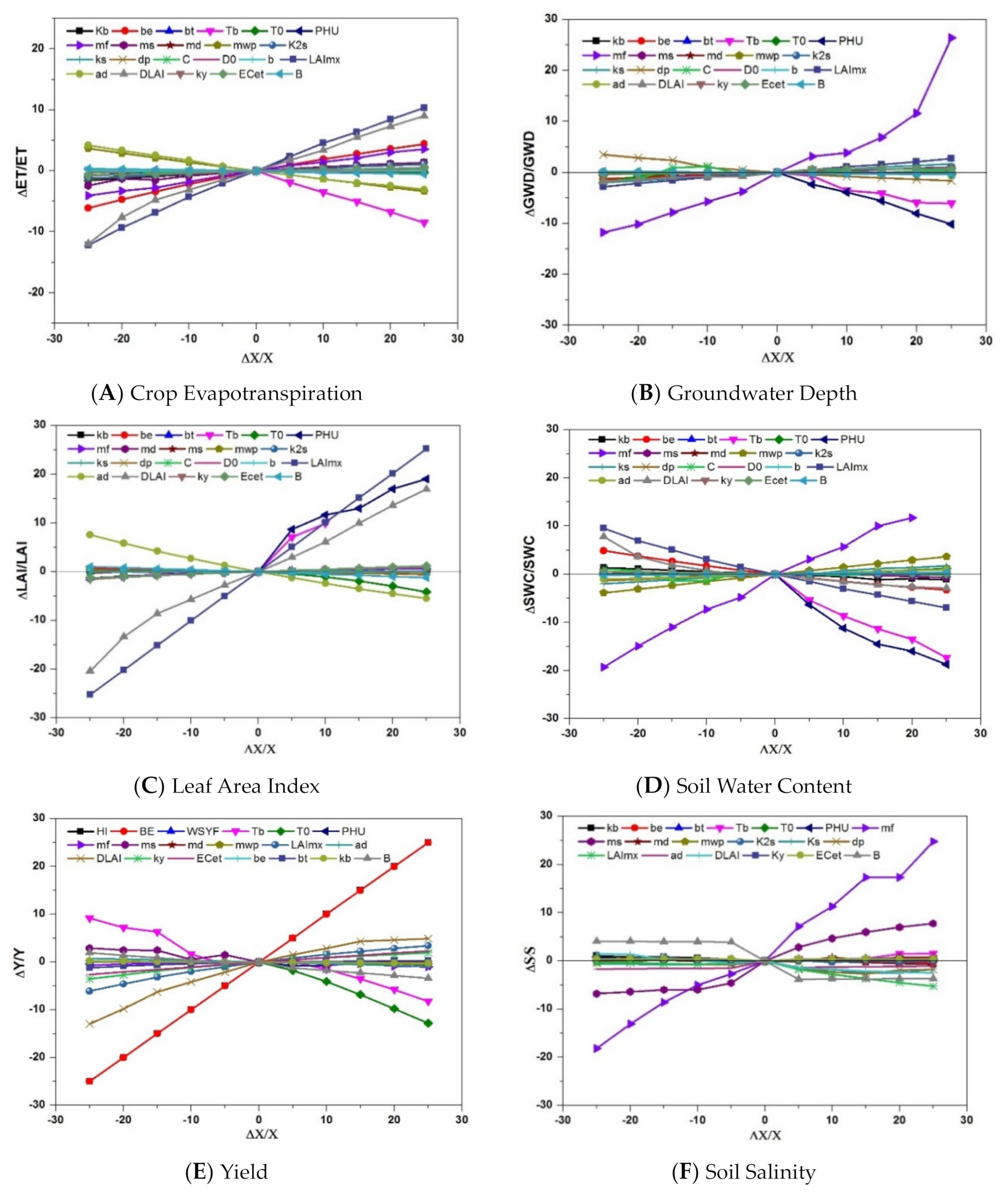
To investigate the effect of calibrated parameters on the crop evapotranspiration, groundwater depth, LAI, soil water content, crop yield and soil salinity of 90 cm soil, the parameters sensitivity and uncertainty were analyzed together (Figure A4). When the parameters varied, the six indexes were linearly related to the change in the parameters, except for the Tb, PHU and C. For the crop evapotranspiration, the LAImx affects the ET most obviously, and then the be and Tb significantly affected the ET (Figure A4A). The other parameters affected the ET slightly when ΔET/ET was less than 5% as the parameters increased by 25%. Most of the parameters had little impact on the ET. The initial LAImx is from the recommended value of the EPIC. Through the calibration and sensitivity of the parameters the final LAI was determined. Detailed information is shown in Figure A4 in the Appendix B.
For the groundwater depth, mf, dp, Tb and PHU are the main impact factors. The others had almost no influence on the groundwater depth (Figure A4B). mf was measured in the field experiment using undisturbed samples. The initial dp was obtained by the recommended value of the local government, and Tb, PHU was obtained by the recommended value of EPIC. Detailed information is shown in Figure A4 in the Appendix B.
Similar to the ET, the main impact factors on LAI are LAImx, Tb, PHU, T0 and ad. The other parameters had little effect on the LAI. The initial Tb, PHU, T0 and ad are recommended by EPIC. Detailed information is shown in Figure A4 in Appendix B.
For the soil water content of 90 cm, parameters such as mf, ms, mwp, LAImx, PHU, Tb affect the soil water content more obviously than the other parameters. mf, ms, and mwp were measured in the experiment. The initial LAImx, PHU, and Tb are recommended by EPIC. Detailed information is shown in Figure A4 in the Appendix B.
For the crop yield, the main impact factors are BE, T0, Tb, DLAI and LAImx. The other parameters had little effect on the yield. The initial BE, T0, Tb, DLAI and LAImx are recommended by EPIC. Detailed information is shown in Figure A4 in the Appendix B.
For a soil salinity of 90 cm, parameters such as mf, B, and ms affect the soil salinity more obviously than the other parameters. mf, ms were measured in the experiment. B is recommended by FAO-56. Detailed information is shown in Figure A4 in the Appendix B.
Combining the observed data, the uncertainty analysis of the parameters of groundwater depth, LAI, soil water content and soil salinity were analyzed (Table 6).
Through the uncertainty analysis of the parameters, the d-factors calculated by Equation (2) ranged from 0 to 1.62 with an average value of 0.17. A larger d-factor represents larger uncertainty. From the data, it can be inferred that for the groundwater depth, LAI, soil water content and soil salinity, the most uncertain parameters are the same with the most sensitive parameter. The most uncertain parameters are mf, LAImx, mf, and mf for groundwater depth, LAI, soil water content and soil salinity, respectively. The trend of uncertainty of the parameters is basically similar to the sensitivity. Detailed information is shown in Table 6.
3.2. Effect of Salinity in Groundwater on Crop Water Use and Yield
3.2.1. Groundwater Recharge on soil Water in Root Zone
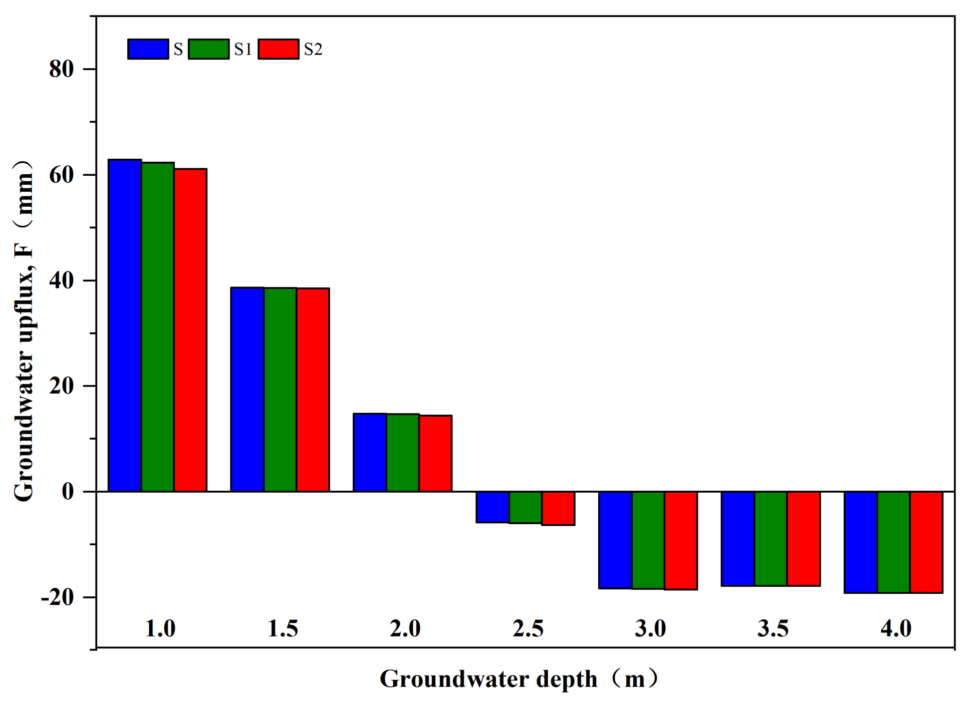
The water flux at the lower boundary (F) of zone 2 is the exchange between groundwater and soil water, as shown in Figure 3. Obviously, groundwater recharge decreases with deeper groundwater, which has been proven in previous studies [15,16]. The results show that groundwater recharge to soil water decreases slightly with increasing groundwater salinity under full irrigation when groundwater depth is shallower than 3 m, while F with groundwater mineralization being 4 g/L is less than that with 1 g/L by 1.67 mm. When groundwater is deeper than 3 m, the effect of groundwater mineralization on F can be neglected, which is related to the relation between groundwater depth and F [31]. In general, regardless of which groundwater depth, the influence of groundwater salinity on groundwater rise is relatively small. Even when the groundwater depth is 1 m, the groundwater rise with a groundwater salinity of 4 g/L is only 2.7% less than that with the groundwater salinity of 1 g/L. In the case of other groundwater depths, the decline rate is smaller.
3.2.2. Soil Salt Content in Actual Root Zone
The variation of average salt in the actual root zone with groundwater depth and mineralization changes throughout the growing period is shown in Figure 4. The results show that with increasing groundwater salinity, the average salt content of the actual root zone increases gradually during the growth period under constant groundwater depth. This increase varies with different groundwater depths. For example, when the groundwater depths are 1 m and 2.5 m, the average salt contents of the actual root zone under groundwater salinity of 1, 2, and 4 g/L are 1.07, 1.15, 1.30 kg/m2 and 1.06, 1.07, 1.10 kg/m2, respectively. The average salt content of the actual root zone increases only by 0.001 kg/m2 under a groundwater depth of 4 m. Therefore, the groundwater depth directly affects the influence of groundwater salinity on the salt content of the actual root zone, which can be indicated in the above text that the groundwater capillary rise and groundwater salinity to the root zone increase with groundwater shallower.
In constrast, the average salt content of the actual root zone decreases with groundwater deeper under the same groundwater salinity, while the average salt content of the actual root zone ranges from 1.30 kg/m2 to 1.07 kg/m2 with groundwater depths varying from 1 m to 4 m under groundwater salinity of 4 g/L. Therefore, extensive study on groundwater depth and groundwater salinity is also an important part of a rational irrigation system [22].
3.2.3. Crop Evapotranspiration
The response of groundwater salinity to crop evapotranspiration under the same irrigation amount is shown in Figure 5A. On one hand, crop evapotranspiration decreases with increasing groundwater salinity under the same groundwater depth. The effect of groundwater salinity on crop evapotranspiration can be neglected when groundwater is deeper than 3 m. For example, crop evapotranspiration increases by 11.53 mm with groundwater salinity from 1 g/L to 4 g/L under groundwater depth of 1.5 m, but this increase is only 0.78 mm under groundwater depth of 3.0 m.
On the other hand, the groundwater recharge to soil water and crop evapotranspiration increases when groundwater is shallower, which indicates that the influence of groundwater depth on crop evapotranspiration is greater than that by average salt of the actual root zone. Xu et al. [48] reported that the groundwater contribution to crop growth was significant when the depth of the groundwater table was less than 1.50 m but was irrelevant for depths greater than 2.00 m. As shown in Figure 5, the crop evapotranspiration increases by 9 mm with groundwater depth ranging from 1.5 m to 1 m under groundwater salinity of 1 g/L, while the average salt of the actual root zone increases with groundwater shallower. With increasing groundwater salinity, the influence of groundwater depth on crop evapotranspiration is almost the same as that of the average salt of the actual root zone. For instance, crop evapotranspiration with groundwater depths of 1 m and 1.5 m under groundwater salinity of 4 g/L are similar.
3.2.4. Maize Yield
The effect of groundwater salinity on crop yield under the same irrigation amount is similar to that on crop evapotranspiration, as shown in Figure 5B. The influence of different groundwater salinities on maize yield mainly comes from two aspects. On one hand, crop yield decreases with increasing groundwater salinity under the same groundwater depth. When groundwater depth is greater than 3 m, this influence can be neglected, while maize yield was 13.07 Mg/ha, 13.06 Mg/ha and 13.04 Mg/ha with groundwater salinity of 1.0 g/L, 2.0 g/L and 4.0 g/L under groundwater depth of 3 m [25].
On the other hand, under same groundwater salinity, maize yield with shallower groundwater is greater than that with deeper groundwater. Maize yield is affected by groundwater depth greater than that by soil salt under low groundwater salinity. For example, maize yield with groundwater depth of 1.0 m under groundwater salinity of 1.0 g/L is greater by 0.1 Mg/ha than that with groundwater depth of 1.5 m, but this increase is only 0.02 Mg/ha under groundwater salinity of 4.0 g/L.
According to the effect of groundwater salinity on maize yield and crop evapotranspiration, the effect of groundwater salinity on the yield is slightly less than that on the crop evapotranspiration when the groundwater salinity is less. Based on the above analysis, when the salinity of groundwater is 1.0 g/L, the water consumption of maize under groundwater depth of 1.0 m increased by 3.6% compared to that under groundwater depth of 2.0 m, but the yield of maize under groundwater depth of 1 m was 1.6% larger than that of 2 m. Therefore, the effect of groundwater salinity on crop yield is slightly less than that on crop water consumption [52].
3.2.5. Water Productivity and Irrigation Water Productivity
Water productivity is the ratio of crop yield to evapotranspiration. The average water productivity is approximately 2.88 kg/m3, while water productivity was 2.83 kg/m3 and 2.90 kg/m3 under groundwater depths of 1 m and 3 m, respectively. The WP declined when the groundwater depth was greater than 3.5 m.
Irrigation water productivity (IWP) is the ratio of maize yield to the amount of irrigation water. Results show that the IWP of maize range from 4.0 kg/m3 to 4.2 kg/m3. The IWP decreases with groundwater deeper, while IWP decreases from 4.16 kg/m3 to 4.04 kg/m3 with groundwater depth ranging from 1 m to 4 m under groundwater salinity of 1 g/L.
4. Discussion
4.1. Contribution of Groundwater Recharge on Crop Water Use
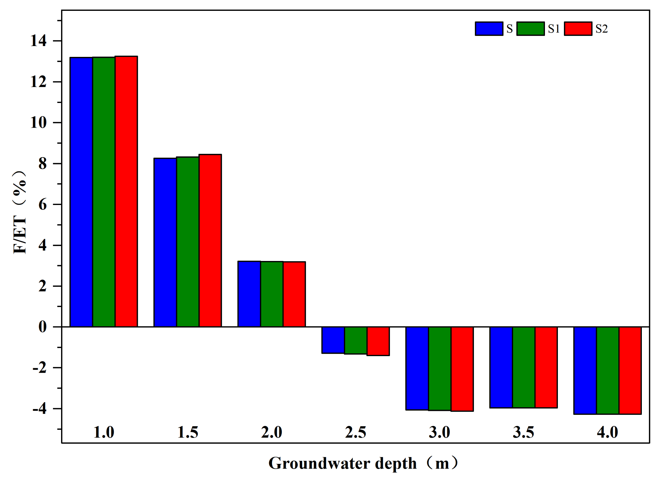
The response of groundwater salinity to groundwater recharge to crop water use is shown in Figure 6. Similar to the findings of Luo and Sophocleous [23], ratios of seasonal groundwater evaporation to seasonal potential ET were plotted against the depth to the water table. When the groundwater was deeper than 3.0 m, the crop ET decreased significantly due to a lack of groundwater upward flux to crop growth under deeper groundwater. When groundwater depth ranges from 1 m to 2 m, the groundwater contribution to crop water use increases slightly with increasing groundwater salinity under the same groundwater depth. As shown in Figure 6, groundwater contributions to crop evapotranspiration with groundwater salinity of 1 g/L is lower than that with 4.0 g/L by 0.15% under groundwater depth of 1 m. This indicates that the influence of groundwater salinity on crop evapotranspiration is slightly greater than that on groundwater recharge. Then, the effect of groundwater depth on groundwater contribution is the important factor. Because of the lower effect of groundwater on soil water and crop evapotranspiration with deeper groundwater, the influence of groundwater salinity on soil water and crop evapotranspiration will decrease [25,53]. Babajimopoulos et al. found that the specific field conditions about 3.6 mm/day of the water in the root zone originated from the shallow water table amounting to about 18% of the water, which was transpired by the maize with the water table observed at a mean depth of 0.58 m below soil surface [54].
4.2. Relationship between WP, IWP and Groundwater Salinity, Groundwater Depth
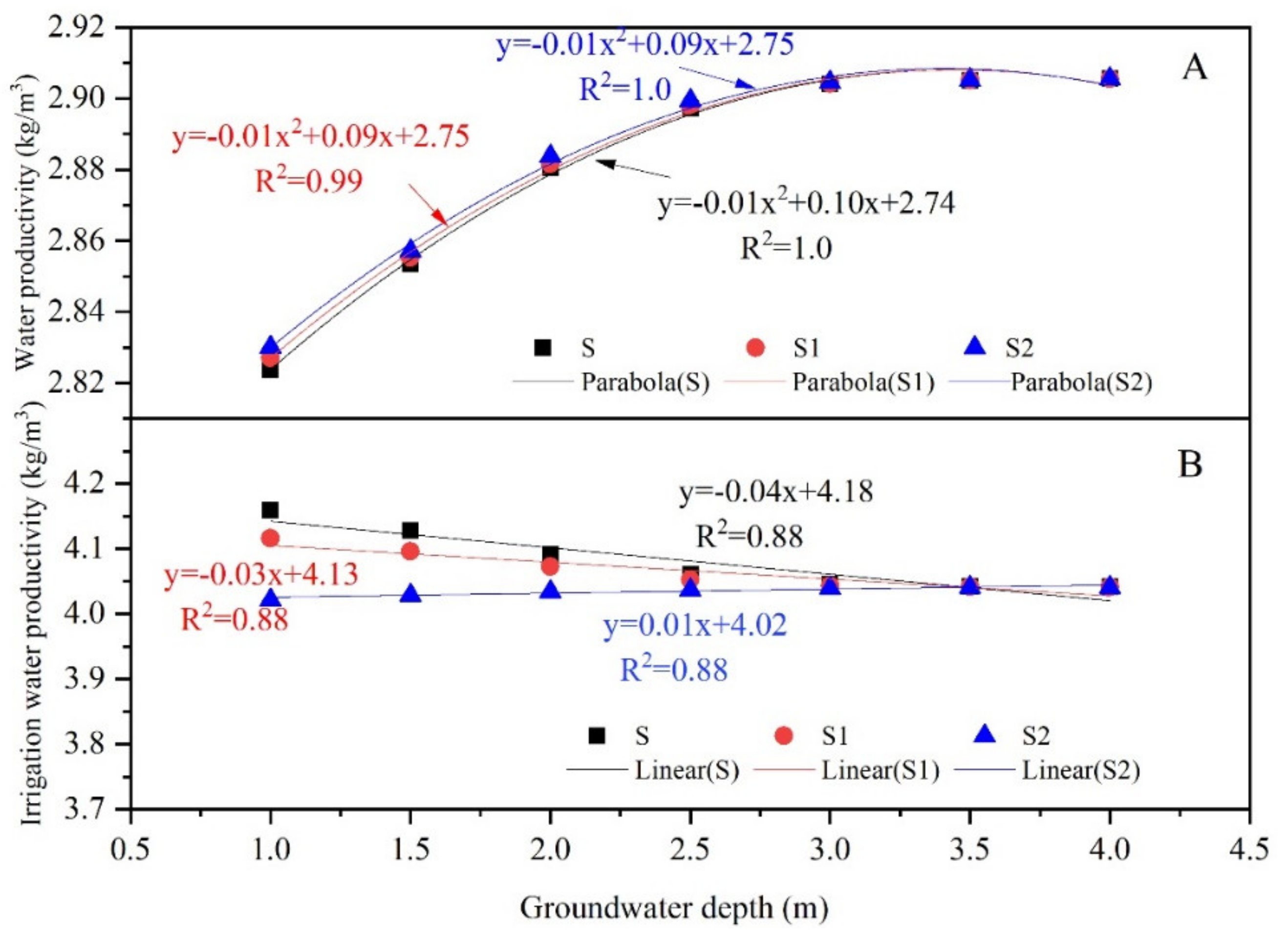
Relationship between WP and groundwater depth and salinity is shown in Figure 7A. The WP declined when the groundwater depth was greater than 3.5 m. However, WP increased mildly with increasing groundwater salinity, especially with shallow groundwater. For example, WP increased by 0.01 kg/m3 with groundwater salinity ranging from 1.0 g/L to 4.0 g/L, which indicates that the effect of salt on crop evapotranspiration is more significant than that on crop yield. The result is similar to the study of Jiang et al. [52] which reported that water productivity irrigated by brackish water is slightly higher than that irrigated by fresh water.
Relationship between IWP and groundwater depth and salinity under same irrigation amounts is shown in Figure 7B. The effect of groundwater on IWP is different from that on WP. Results show that the IWP of maize decreases from 4.16 kg/m3 to 4.04 kg/m3 with groundwater depth ranging from 1 m to 4 m under groundwater salinity of 1 g/L, which is similar to the results of Sun et al. [55]. However, IWP increases gradually with deeper groundwater under groundwater salinity of 4 g/L, which is due to the decline of soil salt from groundwater decline with deeper groundwater. For example, IWP ranges from 4.02 kg/m3 with groundwater depth varying from 1 m to 4 m. Therefore, IWP increases with deeper groundwater when groundwater salinity decreases to a certain extent.
In contrast, IWP decreases with increasing groundwater salinity at the same groundwater depth, especially for shallow groundwater. As shown in the Figure 7, when the groundwater depth is 1 m and 1.5 m, the IWP of maize is 4.16 kg/m3, 4.12 kg/m3, 4.02 kg/m3 and 4.13 kg/m3, 4.10 kg/m3 and 4.03 kg/m3 under groundwater salinity conditions of 1.0 g/L, 2.0 g/L and 4.0 g/L, respectively. It is further proved that the shallower the groundwater depth, the groundwater salinity has a certain inhibition on the yield and has a greater impact on irrigation water productivity. The groundwater salinity is affected by irrigation water quality, soil prosperity, land use and management and so on [56,57].
In addition, the change of WP caused by groundwater level fluctuation is higher than that by groundwater salinity. The WP increased by 0.01 kg/m3 with groundwater salinity ranging from 1.0 g/L to 4.0 g/L under groundwater depth of 1.0 m, while the WP increased by 0.03 kg/m3 with groundwater depth ranging from 1.0 m to 1.5 m under groundwater salinity of 1.0 g/L. However, the change of IWP caused by groundwater level fluctuation and groundwater salinity has not obvious difference. Above results can be attributed to that the effect of capillary rise on crop evapotranspiration is more significant than that on crop yield under shallow groundwater [31,58].
5. Conclusions
The influence of different groundwater salinity on soil salinity, groundwater recharge, crop water use, yield, water use efficiency and other parameters was investigated using the modified AWPM-SG. When the groundwater depth was more than 3 m, the groundwater recharge to soil water had a negative value. Under the same groundwater salinity, soil salinity in the root zone increased with groundwater shallower and maize growth was affected significantly. Under the same salinity, the smaller the groundwater depth, the smaller the water productivity and irrigation water productivity of maize.
Because groundwater salinity has little effect on groundwater recharge and great restraint on the crop water use, the groundwater salinity is higher under the same groundwater depth. Then the contribution of groundwater recharge to crop water consumption increased slowly. In conclusion, the inhibition of soil salt content on maize yield is slightly less than that on maize water consumption. Therefore, under the same groundwater depth, the higher the salinity, the greater the corn water productivity, and the smaller the corn irrigation water productivity. In summary, the effect of groundwater salinity on crop water productivity and irrigation water productivity is not significant. In the future, the modified AWPM-SG can be promoted for similar areas with shallow groundwater.
Author Contributions
Conceptualization, Z.H. and Z.Q.; methodology, X.G. and P.T.; software, X.G.; formal analysis, X.G. and P.T.; data curation, X.G. and S.Q.; writing—original draft preparation, X.G. and P.T.; writing—review and editing, Z.Q.; visualization, X.G.; project administration, X.G.; funding acquisition, Z.Q. and X.G. All authors have read and agreed to the published version of the manuscript.
Funding
This research was funded by project from Start-up Project for Bringing in High-level talent of Inner Mongolia Agricultural University (NDYB2019-6), the National Nature Science Foundation of China (51809142, 51609154), Nature Science Foundation of Inner Mongolia (2020MS05011) and China Postdoctoral Science Foundation (2018M631778).
Acknowledgments
The authors would like to thank the editor and all the reviewers for their insightful comments and constructive suggestions.
Conflicts of Interest
The authors declare no conflict of interest.
Appendix A
Method (Modified AWPM-SG):
A.1. Modified AWPM-SG Model Overview
AWPM-SG incorporates a new crop growth model on WIPE’s original code. It combines the WIPE model (Saleh et al., [44]) with EPIC crop growth model (Williams et al., [47]) to simulate the hydrological processes completely including the soil water flow, water flux at water table and crop growing. In addition, the modified AWPM-SG considers the cycle of soil salinity. The modified AWPM-SG requires various inputs for soil (field capacity, permanent wilting point, residual moisture, saturated water content, saturated hydraulic conductivity), groundwater (drainable porosity), daily weather (minimum and maximum temperature, solar radiation, rainfall), crop (crop-specific base temperature, value of the maximum of crop leaf area index, parameter that governs LAI decline rate for crop, the value of HUI when LAI starts declining, harvest index, reduction in yield per increase in the electrical conductivity of saturation extract (ECe), electrical conductivity of the saturation extract at the threshold of ECe when crop yield first reduces below Ym, a yield response factor), management (irrigation, growing time) and initial conditions (volumetric soil water content, groundwater depth). The modified AWPM-SG needs less demanding data input soil parameters to simulate the groundwater capillary when compared with the SWAP-EPIC model by Xu et al. [48]. The schematic of the modified AWPM-SG is shown in Figure 2.
A.1.1. Description of Crop Module-EPIC Considering Soil Salinity
The EPIC plant growth model was developed to estimate soil productivity as affected by erosion throughout the U.S. The processes simulated include leaf-area index; conversion of biomass; above ground mass; economic yield; root growth and water use.
Phonological Development
In EPIC, phonological development of the crop is based on daily heat unit accumulation. It is computed using the equation:
where HU, Tmx, Tmn are the values of heat units, maximum temperature and minimum temperature in °C for any day K, and Tb is the crop-specific base temperature in °C. A heat unit index (HUI) ranging from 0 at planting to 1 at physiological maturity is calculated as follows:
where HUI is the heat unit index for day i and PHU is the potential heat units required for maturity. The value of PHU may be provided by the user or calculated by the model from normal planting and harvest dates.
Potential Growth
Interception of solar radiation is estimated with a Beer’s law equation (William et al., [43]):
where PAR is intercepted photosynthetic active radiation in MJ/m2, RA is solar radiation in MJ/m2, LAI is the leaf area index, and subscript i indocates the day of the year. The constant, 0.5, is used to convert solar radiation to photosynthetically-active radiation. Experimental studies indicate that the extinction coefficient varies with foliage characteristics, sun angle, row spacing, row direction, and latitude. The value used in EPIC (0.65) is representative of crops with narrow row spacings. A somewhat smaller value (0.4–0.6) might be appropriate for tropical areas in which average sun angle is higher and for wide row spacings. Using Monteith’s approach, potential increase in biomass for a day can be estimated with the following equation:
where is the daily potential increase in biomass in t/ha, BE is the crop parameter for converting energy to biomass in (kg/ha)/(MJ/m2).
A.1.2. Leaf Area Index
Leaf area index (LAI) is simulated as function of heat units, crop stress and crop development stages. From emergence to the start of leaf decline, LAI is estimated with the equation:
where HUF is the heat unit factor, REG is the value of the minimum crop stress factor. is the value of the maximum of crop leaf area index, , are the crop parameters.
From the start of leaf decline to the end of the growing season, LAI is estimated with the equation
where ad is a parameter that governs LAI decline rate for crop and is the value of HUI when LAI starts declining.
A.1.3. Effect of Environmental Stress on Biomass Growth
When an environmental stress factors (soil water, temperature, nitrogen, Phosphorus and so on) is less than 1, actual crop biomass growth is calculated as follows:
where is the actual growth of crop biomass in the i-th day (t/hm2); REG is the value of the minimum crop stress factor.
where WS is water stress factor; TS is temperature stress factor; SS is soil salinity stress factor; is the potential crop evapotranspiration (mm/d); is the actual crop evapotranspiration (mm/d); is the average daily temperature (°C); is the base temperature (°C); is the optimal temperature (°C); ECe is mean electrical conductivity of the saturation extract for the root zone (ms/cm); is electrical conductivity of the saturation extract at the threshold of ECe when crop yield first reduces below maximum expected crop yield (Ym (ms/cm)); Ky is a yield response factor; B is the reduction in yield per increase in ECe [%/(ms/cm)], when crop yield first reduces below Ym; is electrical conductivity of soil solution with soil ratio water of 1:5.
A.1.4. Root Growth
Root length is simulated as function of the heat units and the maximum of root length. The root length will be maximum before the mature stage:
where is the variation of root depth in the ith day (cm); is the root depth in the ith day (cm); is the maximum depth reached by roots (cm).
A.1.5. Crop Yield and Water Productivity
The crop yield considering the water stress can be expressed as the equation:
where WSYF is a parameter expressing the sensitivity of harvest index to drought, WS is the water stress factor. HI is the harvest index. Ba is the crop biomass above ground and calculated by LAI and BE (a conversion factor of crop transferring the energy to biomass).
Water productivity and irrigation water productivity was computed using the following equation:
where WP represents the water use efficiency (WUE, kg/m3), and IWP represents irrigation water use efficiency (kg/m3). Y denotes the final grain yield (kg/ha), ET is the total ET (mm), I is the irrigation amount from planting to harvest (mm).
The input parameters of crop module (Table 4) include daily maximum, minimum and mean value of temperature, Tmax, Tmin and Tmean (°C); crop-specific base temperature, Tb (°C); the potential heat units required for maturity, PHU; the maximum of crop leaf area index, LAImax; the maximum of crop root, RDmx; the crop parameters, ab1, ab2; the parameter that governs LAI decline rate for crop, ad; the value of HUI when LAI starts declining, HUI0; the parameter expressing the sensitivity of harvest index to drought, WYSF; the harvest index, HI (Table 4). The output is daily leaf area index, LAI; crop height, h; root growth, R; crop yield, Y and water productivity, WP, IWP.
A.2. Description of Soil Module-WIPE Considering Soil Salinity
The underground model in this study is a modification of the watershed irrigation potential estimation (WIPE) model designed by Saleh et al. [44] to study the impact of irrigation management schemes on groundwater levels. This is a one-dimensional model employing the Thornthwaite-Mather procedure to calculate the recharge (Steenhuis and van Molen [59]) of the aquifer and is primarily applicable to shallow aquifers. Precipitation, irrigation, soil properties such as the moisture content, soil salinity content and the hydraulic conductivity and the initial groundwater level are required to run this model.
The model begins by dividing the soil profile into four zones namely the current root zone, future root zone, transmission zone, and the saturated zone over an impermeable bed as shown in Figure A3 in the Appendix B. The zone 1 is the zone occupied by roots; the zone 2 is the zone that is not currently occupied by the roots but will be so after their complete development; the zone 3 is the unsaturated transition zone below the root zone with lower boundary at water table and the thickness of this layer varies in time according to extraction/evaporation and recharge; the zone 4 is the saturated zone and is regarded as the water table. The zone 3 is always at the constant moisture content and is equal to the saturated moisture content minus the drainable porosity.
A.2.1. Soil Water Flow
When , water balance is calculated in the zone 1:
when where mf is field capacity
where is water content in the zone 1 (mm); mr, mg are the soil moisture in the zone 1, 2 (cm3/cm3); P is precipitation (mm), I is irrigation (mm), is actual evapotranspiration (mm); is the water depth supplied to the root zone from deeper zone due to the root growth (mm); is the water depths that leave the current root zone (mm); CAP is the capillary rise from zone 2 (mm) (Ritchie, 1996), is the averaged diffusivity of zone 1 (cm2/day); D0 is the diffusivity at wilt pointing of zone 1 (cm2/day); b is the empirical parameter of soil. In the study, the soil texture of zone 1 and zone 2 are same.
A.2.2. Water Balance Calculation of Zone 2:
When mg ≥ mf (field capacity) where mf is the redistribution moisture content of root zone and the flux J is given by (Saleh et al., [44])
which is always directed downwards (mm). Here ms is the saturated moisture content of root zone (cm3/cm3), md is the air dry moisture content of root zone (cm3/cm3), is the saturated hydraulic conductivity of root zone (mm/day), and C is a constant to 13. In this condition, there will be no upward evaporation flux from the aquifer so flux = −J.
When mg < mf there will not be any downward flux so that J = 0. However, the upward evaporative flux from the aquifer will be non-zero and is a function of depth to water table from soil surface as given by Gardner [46]:
where ks is the saturated hydraulic conductivity of transmission zone (mm/day), h is the depth to the water table (mm), αis the diffusivity coefficient which is the inverse of air entry , and is the matric potential calculated as:
The air entry value is calculated using (Saxton et al. [60]):
When the water table is closer to soil surface the flux will be maximum and as water table goes down the flux will decrease. The limiting depth at which the flux becomes zero is approximately 4.5 m below ground level.
Irrigation using groundwater is simulated by extracting water from the aquifer and adding it to root zone. The water table depth is updated as:
where is the extraction rate and dp is the drainable porosity.
where is water content in the zone 2 (mm); mg is the soil moisture in the zone 2 (cm3/cm3). When , there will be no zone 2, the calculation of zone 1 is similar to zone 2 when .
The input parameters of soil module (Table 3) include Saturated moisture, ms; Air-dry moisture, md; Saturated hydraulic conductivity, Ks, constant C, b; the thickness of zone 1 and 2 (maximum root depth), the diffusivity at wilt pointing, D0; initial soil moisture and groundwater depth. The output is daily soil moisture and groundwater depth.
A.2.3. Soil Salt Transport
When , salt balance is calculated in the zone 1:
Salt balance calculation of zone 2:
When mg < mf there will not be any downward flux so that J = 0. The water flux at the boundary of zone 2 is upward. The calculation is as follows:
When mg ≥ mf (field capacity), the flux J is always downward:
where , are the soil salt concentration of zone 1 and zone 2 (mg/L); is the groundwater salt concentration (mg/L); G is the groundwater depth considering the fluctuation of groundwater level (mm). When , there will be no zone 2, the calculation of zone 1 is similar to zone 2 when .
When mg<mf there will not be any downward flux so that J = 0. The water flux at the boundary of zone 2 is upward.
When mg ≥ mf (field capacity), the flux J is always downward:
A.3. Description of Actual Evapotranspiration Considering Soil Salinity
The actual evapotranspiration is calculated and subtracted from soil-water storage. is a fraction of potential evapotransiration, , which consists of potential evaporation from soil, , and potential transpiration from plants, . The ratio of to depends upon the development stage of the leaf canopy, expressed as , the dimensionless fraction of incident beam radiation that penetrates the canopy (Campbell and Norman [61]):
kb is the dimensionless canopy extinction coefficient, with a value of about 0.82 (Stockle [62]) and LAI is leaf-area index, daily values of which can be obtained by simulation of EPIC.
Accordingly, is allocated to:
Actual evapotranspiration, ET (mm), can be limited by the availability of water and salt in the soil. Thus total actual evaporation and transpiration from soil are modeled as Kendy et al. [33] calculate the crop evapotranspiration using this method in the north of China:
where mr is the moisture content of root zone and bt = 3 for transpiration and be = 0.8 for evaporation.
Appendix B
Figure A1.
Average minimum and maximum temperature and rainfall during the crop growing period during 2016 that the experiment was carried in Fenzidi experimental site where it was arid and semi-arid climate.
Figure A1.
Average minimum and maximum temperature and rainfall during the crop growing period during 2016 that the experiment was carried in Fenzidi experimental site where it was arid and semi-arid climate.
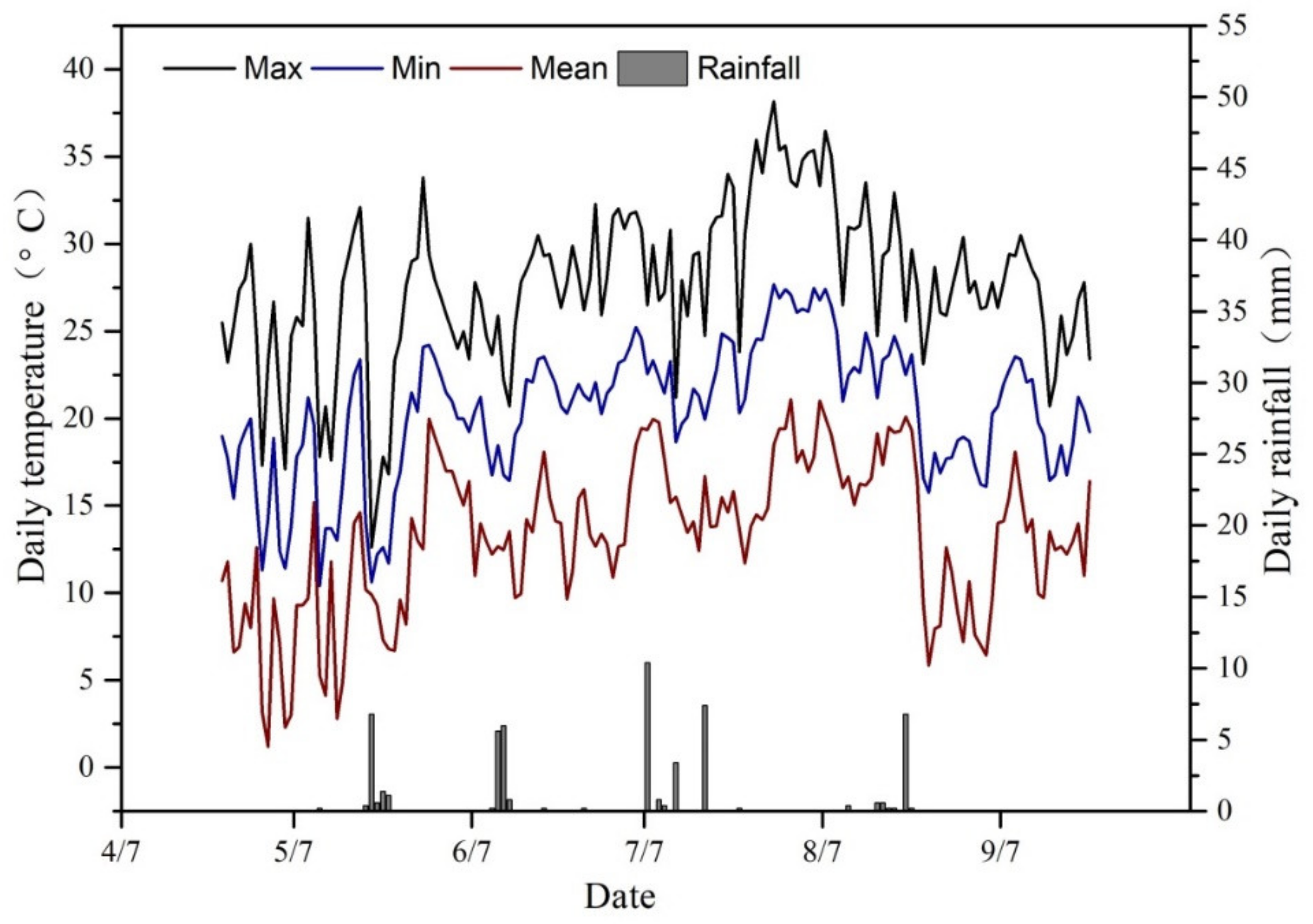
Figure A2.
Contrast between measured soil total salinity and that through regression.

Figure A3.
Schematic of the soil profile used in the AWPM-SG.

Figure A4.
Parameters sensitivity analysis for ET, groundwater depth, LAI, soil water and salt content of 90 cm. Note: (A) is the sensitive analysis for ET, (B) is the sensitive analysis for groundwater depth, (C) is the sensitive analysis for LAI, (D) is the sensitive analysis for soil water content; (E) is the sensitive analysis for maize yield, (F) is the sensitive analysis for soil salt content.
References
- Cai, L.G.; Mao, Z.; Fang, S.X.; Liu, H.S. The Yellow River basin and case study areas. In Water Saving in the Yellow River Basin: Issue and Decision Support Tools in Irrigation; Pereira, L.S., Cai, L.G., Musy, A., Minhas, P.S., Eds.; China Agricultural Press: Beijing, China, 2003; pp. 13–34. [Google Scholar]
- Li, C.; Yang, Z.; Wang, X. Trends of Annual Natural Runoff in the Yellow River Basin. Water Int. 2004, 29, 447–454. [Google Scholar] [CrossRef]
- Dalin, C.; Qiu, H.; Hanasaki, N.; Mauzerall, D.L.; Rodriguez-Iturbe, I. Balancing water resource conservation and food security in China. Proc. Natl. Acad. Sci. USA 2015, 112, 4588–4593. [Google Scholar] [CrossRef] [PubMed] [Green Version]
- Wang, H.; Liu, C.; Zhang, L. Water-saving agriculture in China: An overview. Adv. Agron. 2002, 75, 135–171. [Google Scholar] [CrossRef]
- Wang, X.Q.; Gao, Q.Z.; Lu, Q. Effective use of water resources, and salinity and waterlogging control in the Hetao Irrigation Area of Inner Mongolia. J. Arid Land Resour. Environ. 2005, 19, 118–123. [Google Scholar]
- Wei, C.; Ren, S.; Yang, P.; Wang, Y.; He, X.; Xu, Z.; Wei, R.; Wang, S.; Chi, Y.; Zhang, M. Effects of irrigation methods and salinity on CO2 emissions from farmland soil during growth and fallow periods. Sci. Total. Environ. 2020, 752, 141639. [Google Scholar] [CrossRef]
- Nie, S.; Bian, J.; Zhou, Y. Estimating the Spatial Distribution of Soil Salinity with Geographically Weighted Regression Kriging and Its Relationship to Groundwater in the Western Jilin Irrigation Area, Northeast China. Pol. J. Environ. Stud. 2020, 30, 283–294. [Google Scholar] [CrossRef]
- Yu, Y.; Li, X.; Zhao, C.; Zheng, N.; Jia, H.; Yao, H. Soil salinity changes the temperature sensitivity of soil carbon dioxide and nitrous oxide emissions. Catena 2020, 195, 104912. [Google Scholar] [CrossRef]
- Keesstra, S.; Mol, G.; De Leeuw, J.; Okx, J.; Molenaar, C.; De Cleen, M.; Visser, S. Soil-Related Sustainable Development Goals: Four Concepts to Make Land Degradation Neutrality and Restoration Work. Land 2018, 7, 133. [Google Scholar] [CrossRef] [Green Version]
- Hussain, M.; Ahmad, S.; Hussain, S.; Lal, R.; Ul-Allah, S.; Nawaz, A. Rice in Saline Soils: Physiology, Biochemistry, Genetics, and Management. Adv. Agron. 2018, 148, 231–287. [Google Scholar] [CrossRef]
- Farooq, M.; Hussain, M.; Wakeel, A.; Siddique, K.H.M. Salt stress in maize: Effects, resistance mechanisms, and management. A review. Agron. Sustain. Dev. 2015, 35, 461–481. [Google Scholar] [CrossRef] [Green Version]
- Visser, S.; Keesstra, S.; Maas, G.; De Cleen, M.; Molenaar, C. Soil as a Basis to Create Enabling Conditions for Transitions Towards Sustainable Land Management as a Key to Achieve the SDGs by 2030. Sustainability 2019, 11, 6792. [Google Scholar] [CrossRef] [Green Version]
- Keesstra, S.; Bouma, J.; Wallinga, J.; Tittonell, P.; Smith, P.; Cerdà, A.; Montanarella, L.; Quinton, J.N.; Pachepsky, Y.; Van Der Putten, W.H.; et al. The significance of soils and soil science towards realization of the United Nations Sustainable Development Goals. SOIL 2016, 2, 111–128. [Google Scholar] [CrossRef] [Green Version]
- Keesstra, S.; Geissen, V.; Mosse, K.; Piiranen, S.; Scudiero, E.; Leistra, M.; Van Schaik, L. Soil as a filter for groundwater quality. Curr. Opin. Environ. Sustain. 2012, 4, 507–516. [Google Scholar] [CrossRef]
- Gao, X.; Bai, Y.; Huo, Z.; Xu, X.; Huang, G.; Xia, Y.; Steenhuis, T.S. Deficit irrigation enhances contribution of shallow groundwater to crop water consumption in arid area. Agric. Water Manag. 2017, 185, 116–125. [Google Scholar] [CrossRef]
- Gao, X.Y.; Huo, Z.L.; Qu, Z.Y.; Bai, Y.N.; Huang, G.H.; Xu, X.; Huang, G.H.; Xia, Y.H.; Steenhuis, T.S. Modeling contribution of shallow groundwater to evapotranspiration and yield of maize in an arid irrigation district using readily available data. Sci. Rep. 2017, 7, 1–13. [Google Scholar]
- Termeh, S.V.R.; Khosravi, K.; Sartaj, M.; Keesstra, S.D.; Tsai, F.T.-C.; Dijksma, R.; Pham, B.T. Optimization of an adaptive neuro-fuzzy inference system for groundwater potential mapping. Hydrogeol. J. 2019, 27, 2511–2534. [Google Scholar] [CrossRef]
- Ragab, R.A.; El-Ghamry, W.M.; Amer, F. The Conjunctive Use of Rainfall and Shallow Water Table in Meeting Water Requirements of Faba Bean. J. Agron. Crop. Sci. 1988, 160, 47–53. [Google Scholar] [CrossRef]
- Khandker, M.H.K. Crop Growth and Water Use from Saline Water Tables. Ph.D. Thesis, University of Newcastle upon Tyne, Newcastle, UK, 1994; pp. 84–93. [Google Scholar]
- Ayars, J.; Schoneman, R.A. Irrigating field crops in the presence of saline groundwater. Irrig. Drain. 2006, 55, 265–279. [Google Scholar] [CrossRef]
- Gowing, J.; Rose, D.; Ghamarnia, H. The effect of salinity on water productivity of wheat under deficit irrigation above shallow groundwater. Agric. Water Manag. 2009, 96, 517–524. [Google Scholar] [CrossRef]
- Fan, Y.; Miguez-Macho, G. Potential groundwater contribution to Amazon evapotranspiration. Hydrol. Earth Syst. Sci. 2010, 14, 2039–2056. [Google Scholar] [CrossRef] [Green Version]
- Luo, Y.; Sophocleous, M. Seasonal groundwater contribution to crop-water use assessed with lysimeter observations and model simulations. J. Hydrol. 2010, 389, 325–335. [Google Scholar] [CrossRef]
- Gao, X.; Huo, Z.; Bai, Y.; Feng, S.; Huang, G.; Shi, H.; Qu, Z. Soil salt and groundwater change in flood irrigation field and uncultivated land: A case study based on 4-year field observations. Environ. Earth Sci. 2014, 73, 2127–2139. [Google Scholar] [CrossRef]
- Kahlown, M.; Ashraf, M.; Haq, Z.-U. Effect of shallow groundwater table on crop water requirements and crop yields. Agric. Water Manag. 2005, 76, 24–35. [Google Scholar] [CrossRef]
- Pan, Y.; Yuan, C.; Jing, S. Simulation and optimization of irrigation schedule for summer maize based on SWAP model in saline region. Int. J. Agric. Biol. Eng. 2020, 13, 117–122. [Google Scholar] [CrossRef]
- Silva, J.A.; Šimůnek, J.; McCray, J.E. A Modified HYDRUS Model for Simulating PFAS Transport in the Vadose Zone. Water 2020, 12, 2758. [Google Scholar] [CrossRef]
- Metternicht, G.; Zinck, J. Remote sensing of soil salinity: Potentials and constraints. Remote Sens. Environ. 2003, 85, 1–20. [Google Scholar] [CrossRef]
- Mejia, M.N.; Madramootoo, C.A.; Broughton, R.S. Influence of groundwater table management on corn and soybean yield. Agric. Water Manag. 2000, 46, 73–89. [Google Scholar] [CrossRef]
- Wang, Q.J.; Wang, W.Y.; Lu, D.Q.; Wang, Z.R.; Zhang, J.F. Water and salt transport features for salt-effected soil through drip irrigation under film. Trans. Chin. Soc. Agric. Eng. 2000, 16, 54–57. [Google Scholar]
- Huo, Z.; Feng, S.; Huang, G.; Zheng, Y.; Wang, Y.; Guo, P. Effect of groundwater level depth and irrigation amount on water fluxes at the groundwater table and water use of wheat. Irrig. Drain. 2011, 61, 348–356. [Google Scholar] [CrossRef]
- Scanlon, B.R.; Healy, R.W.; Cook, P.G. Choosing appropriate techniques for quantifying groundwater recharge. Hydrogeol. J. 2002, 10, 18–39. [Google Scholar] [CrossRef]
- Kendy, E.; Gérard-Marchant, P.; Walter, M.T.; Zhang, Y.; Liu, C.; Steenhuis, T.S. A soil-water-balance approach to quantify groundwater recharge from irrigated cropland in the North China Plain. Hydrol. Process. 2003, 17, 2011–2031. [Google Scholar] [CrossRef]
- Yang, J.; Wan, S.; Deng, W.; Zhang, G. Water fluxes at a fluctuating water table and groundwater contributions to wheat water use in the lower Yellow River flood plain, China. Hydrol. Process. 2007, 21, 717–724. [Google Scholar] [CrossRef]
- Simunek, J.; Van Genuchten, M.; Sejia, M. The HYDRUS-1D Software Package for Simulating the One-Dimensional Movement of Water, Heat and Multiple Solutes in Variability-Saturated Media. Hydrus Softw. 2005, 68. Available online: https://www.pc-progress.com/Downloads/Pgm_hydrus1D/HYDRUS1D-4.08.pdf (accessed on 14 December 2020).
- Prathapar, S.A.; Qureshi, A.S. Modelling the Effects of Deficit Irrigation on Soil Salinity, Depth to Water Table and Transpiration in Semi-arid Zones with Monsoonal Rains. Int. J. Water Resour. Dev. 1999, 15, 141–159. [Google Scholar] [CrossRef]
- Healy, R.W.; Cook, P.G. Using groundwater levels to estimate recharge. Hydrogeol. J. 2002, 10, 91–109. [Google Scholar] [CrossRef]
- Ayars, J.; Christen, E.W.; Soppe, R.W.; Meyer, W.S. The resource potential of in-situ shallow ground water use in irrigated agriculture: A review. Irrig. Sci. 2005, 24, 147–160. [Google Scholar] [CrossRef]
- Gao, X.Y. Modeling Agricultural Water Productivity in Shallow Groundwater Area. Ph.D. Thesis, China Agricultural University, Beijing, China, 2017. [Google Scholar]
- Wit, K. Apparatus for Measuring Hydraulic Conductivity of Undisturbed Soil Samples. Permeability Capillarity Soils 2009, 72. [Google Scholar] [CrossRef]
- Valdes, R.; Miralles, J.; Franco, J.; Sánchez-Blanco, M.; Banon, S. Using soil bulk electrical conductivity to manage saline irrigation in the production of potted poinsettia. Sci. Hortic. 2014, 170, 1–7. [Google Scholar] [CrossRef]
- Leao, T.P.; Perfect, E.; Tyner, J.S. New semi-empirical formulae for predicting soil solution conductivity from dielectric properties at 50MHz. J. Hydrol. 2010, 393, 321–330. [Google Scholar] [CrossRef]
- Williams, J.R. The EPIC Model. Computer Models of Watershed Hydrology. 909–1000; Singh, V.P., Ed.; Water Resources Publications: Highland Ranch, CO, USA, 1995. [Google Scholar]
- Saleh, A.F.M.; Steenhuis, T.S.; Walter, M.F. Groundwater Table Simulation under Different Rice Irrigation Practices. J. Irrig. Drain. Eng. 1989, 115, 530–544. [Google Scholar] [CrossRef]
- Wang, X.C.; Li, J. Evaluation of crop yield and soil water estimates using the EPIC model for the Loess Plateau of China. Math. Comput. Model. 2010, 51, 1390–1397. [Google Scholar] [CrossRef]
- Gardner, W.R. Some steady-state solutions of the unsaturated moisture flow equation with application to evaporation from a water table. Soil Sci. 1958, 85, 228–232. [Google Scholar] [CrossRef]
- Williams, J.R.; Wang, E.; Meinardus, A.; Harman, W.L.; Siemers, M.; Atwood, J.D. EPIC Users Guide v. 0509; Blackland Research and Extension Center: Temple, TX, USA, 2006. [Google Scholar]
- Xu, X.; Sun, C.; Qu, Z.; Huang, Q.; Ramos, T.B.; Huang, G. Groundwater Recharge and Capillary Rise in Irrigated Areas of the Upper Yellow River Basin Assessed by an Agro-Hydrological Model. Irrig. Drain. 2015, 64, 587–599. [Google Scholar] [CrossRef]
- Moriasi, D.N.; Arnold, J.G.; Van Liew, M.W.; Bingner, R.L.; Harmel, R.D.; Veith, T.L. Model Evaluation Guidelines for Systematic Quantification of Accuracy in Watershed Simulations. Trans. ASABE 2007, 50, 885–900. [Google Scholar] [CrossRef]
- Abbaspour, K.C.; Johnson, A.; van Genuchten, M.T. Estimating uncertain flow and transport parameters using a sequential uncertainty fitting procedure. Vadose Zone J. 2004, 3, 1340–1350. [Google Scholar] [CrossRef]
- Talebizadeh, M.; Moridnejad, A. Uncertainty analysis for the forecast of lake level fluctuations using ensembles of ANN and ANFIS models. Expert Syst. Appl. 2011, 38, 4126–4135. [Google Scholar] [CrossRef]
- Jiang, J.; Feng, S.-Y.; Sun, Z.; Huo, Z. Effects of non-sufficient irrigation with saline water on soil water-salt distribution and spring corn yield. Ying Yong Sheng Tai Xue Bao J. Appl. Ecol. 2008, 19, 2637–2642. [Google Scholar]
- Masoud, M.; Schumann, S.; Mogheeth, S.A. Estimation of groundwater recharge in arid, data scarce regions; an approach as applied in the EI Hawashyia basin and Ghazala sub-basin (Gulf of Suez, Egypt). Environ. Earth Sci. 2013, 69, 103–117. [Google Scholar] [CrossRef]
- Babajimopoulos, C.; Panoras, A.; Georgoussis, H.; Arampatzis, G.; Hatzigiannakis, E.; Papamichail, D. Contribution to irrigation from shallow water table under field conditions. Agric. Water Manag. 2007, 92, 205–210. [Google Scholar] [CrossRef]
- Sun, H.-Y.; Liu, C.-M.; Zhang, X.-Y.; Shen, Y.-J.; Zhang, Y.-Q. Effects of irrigation on water balance, yield and WUE of winter wheat in the North China Plain. Agric. Water Manag. 2006, 85, 211–218. [Google Scholar] [CrossRef]
- Narany, T.S.; Aris, A.Z.; Sefie, A.; Keesstra, S. Detecting and predicting the impact of land use changes on groundwater quality, a case study in Northern Kelantan, Malaysia. Sci. Total. Environ. 2017, 599, 844–853. [Google Scholar] [CrossRef] [PubMed]
- Keesstra, S.; Kondrlovà, E.; Czajka, A.; Seeger, M.; Maroulis, J. Assessing riparian zone impacts on water and sediment movement: A new approach. Neth. J. Geosci. 2012, 91, 245–255. [Google Scholar] [CrossRef]
- Mueller, L.; Behrendt, A.; Schalitz, G.; Schindler, U. Above ground biomass and water use efficiency of crops at shallow groundwater tables in a temperate climate. Agric. Water Manag. 2005, 75, 117–136. [Google Scholar] [CrossRef]
- Steenhuis, T.S.; Van Der Molen, W.H. The Thornthwaite-mather procedure as a simple engineering method to predict recharge. J. Hydrol. 1985, 84, 221–229. [Google Scholar] [CrossRef]
- Saxton, K.E.; Rawls, W.J.; Romberger, J.S. Estimating generalized soil-water characteristics. Soil Sci. Soc. Am. J. 1986, 50, 1301–1306. [Google Scholar] [CrossRef]
- Campbell, G.S.; Norman, J.M. An Introduction to Environmental Biophysics, 2nd ed.; Springer: New York, NY, USA, 1998; p. 249. [Google Scholar]
- Stockle, C.O. Simulation of the Effect of Water and Nitrogen Stress on Growth and Yield of Spring Wheat. Ph.D. Dissertation, Washington State University, Pullman, WA, USA, 1985. [Google Scholar]
Figure 1.
The schematic of the soil water balance calculation and crop growth in the modified AWPM-SG model.
Figure 1.
The schematic of the soil water balance calculation and crop growth in the modified AWPM-SG model.
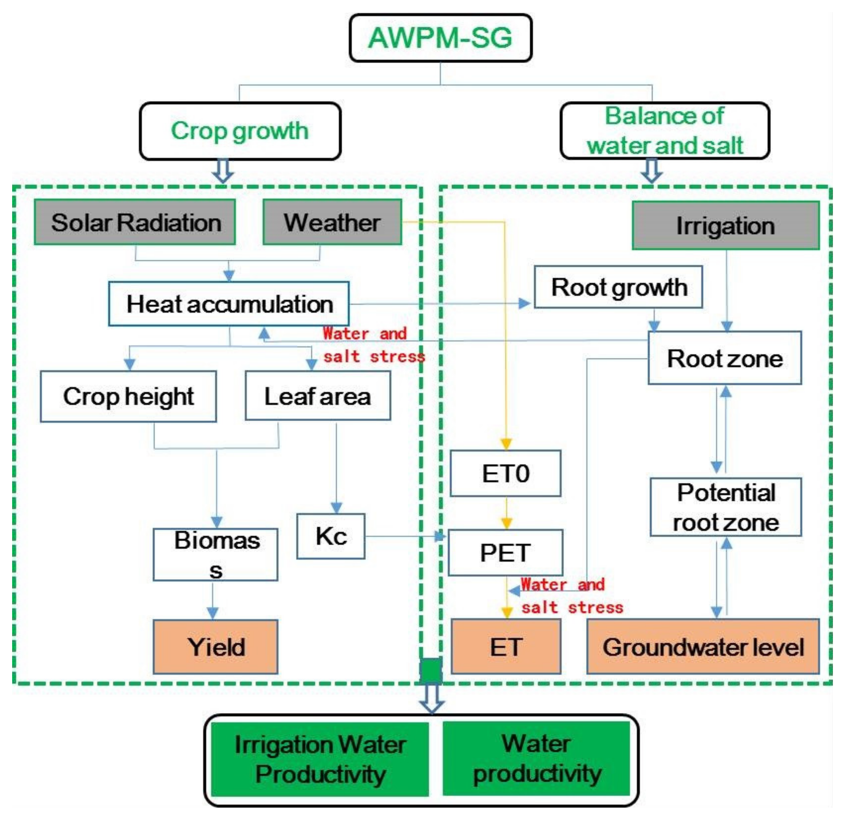
Figure 2.
(A–D) Simulated versus measured soil water content, soil salinity, groundwater depth and leaf area index under different groundwater depths during calibration in S1 and validation in S2. (A) is that simulated versus measured soil water content, (B) is that simulated versus measured soil salinity, (C) is that simulated versus measured groundwater depth and (D) is that simulated versus measured leaf area index.

Figure 3.
Water fluxes at water table during the growing period with groundwater depth ranging from 1 m to 4 m and groundwater salinity ranging from 1 to 4 g/L. Note: S, S1 and S2 refer to the scenarios with groundwater salinity of 1, 2 and 4 g/L, respectively.
Figure 3.
Water fluxes at water table during the growing period with groundwater depth ranging from 1 m to 4 m and groundwater salinity ranging from 1 to 4 g/L. Note: S, S1 and S2 refer to the scenarios with groundwater salinity of 1, 2 and 4 g/L, respectively.

Figure 4.
Soil salt content in root zone during the growing period with groundwater depth ranging from 1 m to 4 m and groundwater salinity ranging from 1 to 4 g/L. Note: S, S1 and S2 refer to the scenarios with groundwater salinity of 1, 2 and 4 g/L, respectively.
Figure 4.
Soil salt content in root zone during the growing period with groundwater depth ranging from 1 m to 4 m and groundwater salinity ranging from 1 to 4 g/L. Note: S, S1 and S2 refer to the scenarios with groundwater salinity of 1, 2 and 4 g/L, respectively.

Figure 5.
Actual crop evapotranspiration of maize and yield during the growing period under various groundwater depths and groundwater salinity. (A) Actual crop evapotranspiration of maize during the growing period with groundwater depth ranging from 1 m to 4 m and groundwater salinity ranging from 1 g/L to 4 g/L. (B) Crop yield during the growing period with groundwater depth ranging from 1 m to 4 m and groundwater salinity ranging from 1 g/L to 4 g/L. Note: ET is actual crop evapotranspiration. S, S1 and S2 refer to the scenarios with groundwater salinity of 1 g/L, 2 g/L and 4 g/L, respectively.
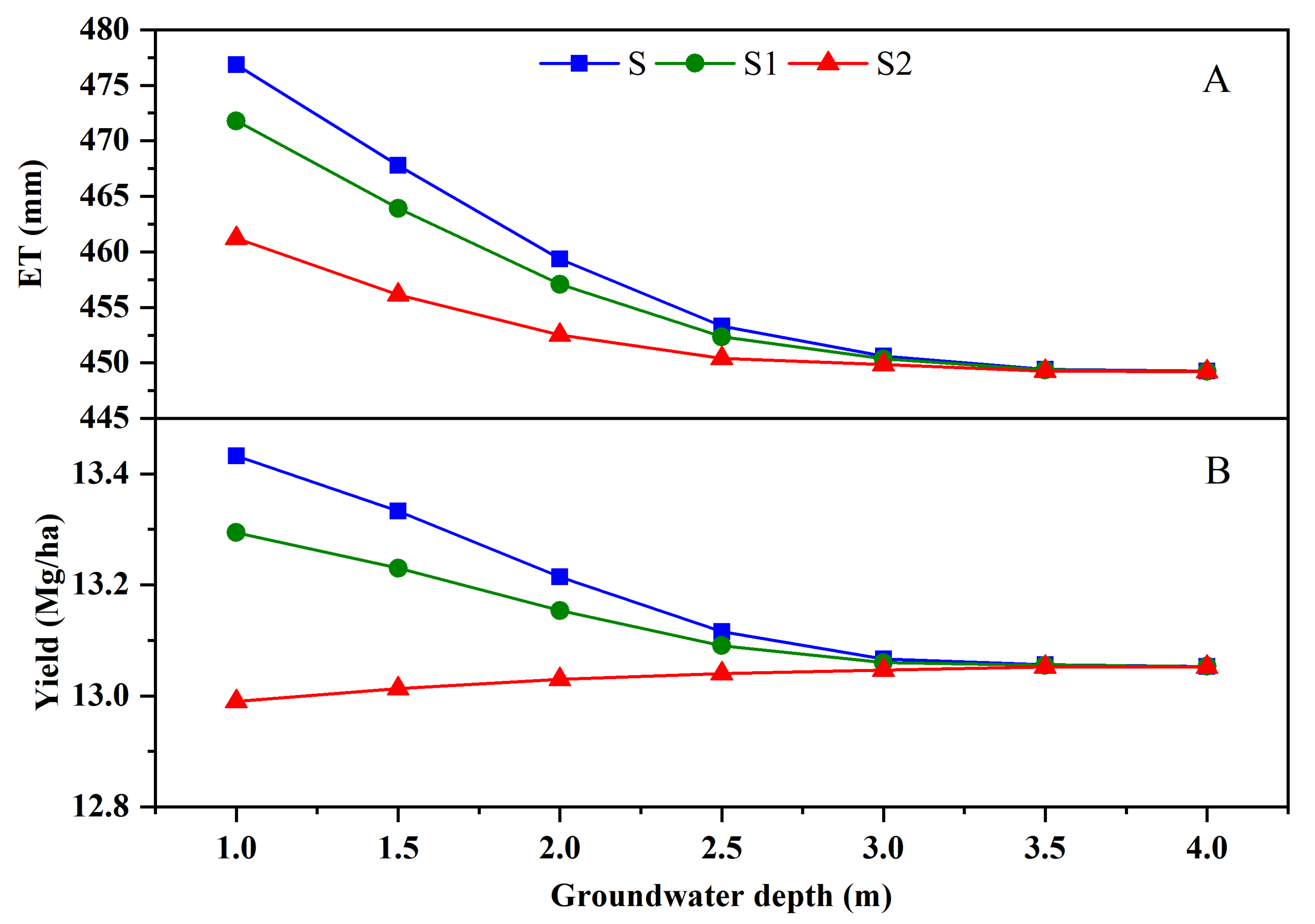
Figure 6.
Groundwater contribution to water use (F/ET) during the growing period with groundwater depth ranging from 1 m to 4 m and groundwater salinity ranging from 1 g/L to 4 g/L. Note: S, S1 and S2 refer to the scenarios with groundwater salinity of 1 g/L, 2 g/L and 4 g/L, respectively.
Figure 6.
Groundwater contribution to water use (F/ET) during the growing period with groundwater depth ranging from 1 m to 4 m and groundwater salinity ranging from 1 g/L to 4 g/L. Note: S, S1 and S2 refer to the scenarios with groundwater salinity of 1 g/L, 2 g/L and 4 g/L, respectively.

Figure 7.
Relationship between water productivity, irrigation water productivity and groundwater depth, groundwater salinity. Note: (A) Relationship between water productivity and groundwater depth, groundwater salinity. (B) Relationship between irrigation water productivity and groundwater depth, groundwater salinity. Note: S, S1 and S2 refer to the scenarios with groundwater salinity of 1, 2 and 4 g/L, respectively.


Table 1.
Irrigation date and amount in Fenzidi in 2016.
| Crop | Date | Irrigation Amount (mm) | |
|---|---|---|---|
| F1 | F2 | ||
| Maize | 7/13 | 114.91 | 118.84 |
| Maize | 7/26 | 86.11 | 86.11 |
| Maize | 8/8 | 122.04 | 122.04 |
Table 2.
Soil physical properties of experimental area.
| Soil Depths (cm) | Soil Particle Size Distribution | Soil Texture | Bulk Density (g/cm3) | Field Capacity,mf (cm3/cm3) | Wilting Point (cm3/cm3) | ||
|---|---|---|---|---|---|---|---|
| Clay (<0.002 mm) | Silt (0.002–0.05 mm) | Sand (0.05–2.0 mm) | |||||
| 0–90 | 15 | 75.14 | 9.86 | Silty loam | 1.41 | 0.32 | 0.04 |
| 90–150 | 4.01 | 56.56 | 39.43 | Silty loam | 1.45 | 0.30 | 0.06 |
Table 3.
Values of hydrological parameters for modified AWPM-SG.
| Depth (cm) | Soil Typer | ms | md | ks | C | dp | D0 | b |
|---|---|---|---|---|---|---|---|---|
| (cm3/cm3) | (cm3/cm3) | (cm/d) | ||||||
| Initial values | ||||||||
| 0–90 | Sandy loam | 0.395 | 0.07 | 30 | 8 | 0.58 | 35.2 | |
| 90–150 | Sandy loam | 0.45 | 0.07 | 80 | 0.08 | |||
| Calibrated values | ||||||||
| 0–90 | Sandy loam | 0.43 | 0.08 | 30 | 13 | 0.1 | 17.5 | |
| 90–150 | Sandy loam | 0.56 | 0.08 | 86 | 0.08 |
Note: ms, md are the saturated moisture, residual moisture of 0–90 cm soil, respectively; ks is the saturated hydraulic conductivity; C, b are the content of soil in zone 1 and 2; D0 is the diffusion rate at wilting point; dp is the drainable porosity.
Table 4.
Default and calibrated values of maize’s physiological parameters for the crop growth part of modified AWPM-SG.
Table 4.
Default and calibrated values of maize’s physiological parameters for the crop growth part of modified AWPM-SG.
| Parameters | Default Values | Calibrated Values |
|---|---|---|
| Dimensionless canopy, kb | 0.5 | 0.8 |
| be | 0.3 | 0.5 |
| bt | 4 | 4 |
| Minimun temperature for plant growth, Tb (°C) | 8 | 8 |
| Optimal temperature for plant growth, T0 (°C) | 25 | 25 |
| Leaf area index decline rate, ad | 1.0 | 0.75 |
| Maximum crop height, hmx (cm) | 250 | 340 |
| Maximum leaf area index, LAImx | 6.0 | 8.2 |
| Maximum root depth, RDmx (cm) | 90 | 90 |
| Plant radiation-use efficienc, BE ((kg×)/(MJ×)) | 40 | 40 |
| Harvest index, HI | 0.5 | 0.4 |
| Total potential heat units required for crop maturation, PHU (℃) | 2000 | 2100 |
| A parameter expressing the sensitivity of harvest index to drought, WYSF | 0.05 | 0.05 |
| reduction in yield per increase in ECe (%/(ms cm−1)) | 12 | 12 |
| electrical conductivity of the saturation extract at the threshold of ECe when crop yield first reduces below Ym (ms cm−1) | 1.7 | 1.7 |
| a yield response factor | 1.25 | 1.25 |
Table 5.
Mean relative error, Root mean square error, Regression coefficient, Nash and Sutcliffe model efficiency and Coefficient of determination of the model calibration and validation.
Table 5.
Mean relative error, Root mean square error, Regression coefficient, Nash and Sutcliffe model efficiency and Coefficient of determination of the model calibration and validation.
| Root Mean Square Error, RMSE | Nash and Sutcliffe Model Efficiency, NSE | Mean Relative Error, MRE (%) | Coefficient of Determination, R2 | Regression Coefficient, b | ||
|---|---|---|---|---|---|---|
| Calibration | Soil water content (cm) | 2.66 | 0.49 | −1.07 | 0.99 | 0.99 |
| Soil salinity (g/L) | 0.26 | 0.85 | −2.57 | 0.90 | 0.96 | |
| Groundwater depth (m) | 0.2 | 0.56 | 0.85 | 0.57 | 0.99 | |
| LAI | 0.42 | 0.97 | −8.4 | 0.99 | 0.93 | |
| Validation | Soil water content (cm) | 1.56 | 0.28 | 1.61 | 1 | 1.01 |
| Soil salinity (g/L) | 0.34 | 0.17 | −7.12 | 0.57 | 0.92 | |
| Groundwater depth (m) | 0.33 | −0.02 | −2.63 | 0.19 | 0.92 | |
| LAI | 0.82 | 0.85 | 14.03 | 0.95 | 1.15 |
Table 6.
Uncertainty analysis of parameters for modified AWPM-SG.
| d-Factor | Parameter | ||||||||||
|---|---|---|---|---|---|---|---|---|---|---|---|
| mf | ms | md | mwp | k2s | ks | C | D0 | b | dp | LAImx | |
| Groundwater depth | 1.44 | 0.38 | 0.03 | 0.006 | 0.07 | 0.2 | 0.15 | 0 | 0.002 | 0.18 | 0.2 |
| LAI | 0.006 | 0.002 | 0 | 0.003 | 0 | 0 | 0 | 0 | 0 | 0 | 0.56 |
| Soil water content | 0.72 | 0.28 | 0.02 | 0.07 | 0.07 | 0.12 | 0.11 | 0 | 0.001 | 0.06 | 0.29 |
| Soil salinity | 1.62 | 1.25 | 0.25 | 0.15 | 0.32 | 0.45 | 0 | 0 | 0 | 0.55 | 0.38 |
| ad | DLAI | Tb | T0 | kb | be | bt | PHU | Ky | ECet | B | |
| Groundwater depth | 0 | 0.09 | 0.38 | 0.07 | 0.03 | 0.08 | 0.008 | 0.45 | 0.053 | 0.052 | 0.03 |
| LAI | 0.11 | 0.46 | 0.29 | 0.19 | 0 | 0.003 | 0.008 | 0.39 | 0 | 0 | 0 |
| Soil water content | 0.04 | 0.15 | 0.14 | 0.03 | 0.06 | 0.11 | 0.01 | 0.18 | 0.005 | 0.006 | 0.01 |
Note: In the uncertainty analysis, larger d-factor represents larger uncertainty of parameters. mf, ms, md, mwp are the field capacity, saturated moisture, residual moisture, wilting moisture of 0–90 cm soil, respectively; k2s is the saturated hydraulic conductivity in zone 1; ks is the saturated hydraulic conductivity in zone 2; C, b are the content of soil in zone 1 and 2; D0 is the diffusion rate at wilting point; dp is the drainable porosity; LAImx is the maximum of crop leaf area index; ad is a parameter that governs LAI decline rate for crop; DLAI is ratio that period from leaf area beginning to decline to whole growing period; Tb is the minimun temperature for plant growth, T0 is the optimal temperature for plant growth; kb dimensionless canopy extinction coefficient; be, bt are the parameters for evaporation and transpiration; PHU is total potential heat units required for crop maturation.
Publisher’s Note: MDPI stays neutral with regard to jurisdictional claims in published maps and institutional affiliations. |
© 2020 by the authors. Licensee MDPI, Basel, Switzerland. This article is an open access article distributed under the terms and conditions of the Creative Commons Attribution (CC BY) license (http://creativecommons.org/licenses/by/4.0/).
Share and Cite
MDPI and ACS Style
Gao, X.; Qu, Z.; Huo, Z.; Tang, P.; Qiao, S. Understanding the Role of Shallow Groundwater in Improving Field Water Productivity in Arid Areas. Water 2020, 12, 3519. https://doi.org/10.3390/w12123519
AMA Style
Gao X, Qu Z, Huo Z, Tang P, Qiao S. Understanding the Role of Shallow Groundwater in Improving Field Water Productivity in Arid Areas. Water. 2020; 12(12):3519. https://doi.org/10.3390/w12123519
Chicago/Turabian StyleGao, Xiaoyu, Zhongyi Qu, Zailin Huo, Pengcheng Tang, and Shuaishuai Qiao. 2020. "Understanding the Role of Shallow Groundwater in Improving Field Water Productivity in Arid Areas" Water 12, no. 12: 3519. https://doi.org/10.3390/w12123519
Note that from the first issue of 2016, this journal uses article numbers instead of page numbers. See further details here.