Modeling Travel Time Distributions of Preferential Subsurface Runoff, Deep Percolation and Transpiration at A Montane Forest Hillslope Site


Department of Hydraulics and Hydrology, Faculty of Civil Engineering, Czech Technical University in Prague, Thakurova 7, 166 29 Prague, Czech Republic
*
Author to whom correspondence should be addressed.
Water 2019, 11(11), 2396; https://doi.org/10.3390/w11112396
Submission received: 15 October 2019
/
Revised: 6 November 2019
/
Accepted: 13 November 2019
/
Published: 15 November 2019
(This article belongs to the Special Issue Hillslope Hydrology: Towards Improved Process Understanding Using Modeling and/or Field Observations)
Abstract
:Residence and travel times of water in headwater catchments, or their smaller spatial units, such as individual hillslopes, represent important descriptors of catchments’ hydrological regime. In this study, travel time distributions and residence times were evaluated for a montane forest hillslope site. A two-dimensional dual-continuum model, previously validated on water flow and oxygen-18 data, was used to simulate the seasonal soil water regime and selected major rainfall–runoff events observed at the hillslope site. The model was subsequently used to generate hillslope breakthrough curves of a fictitious conservative tracer applied at the hillslope surface in the form of the Dirac impulse. The simulated tracer breakthroughs allowed us to estimate the travel time distributions of soil water associated with the episodic subsurface stormflow, deep percolation and transpiration, thus yielding partial travel time distributions for the individual discharge processes. The travel time distributions determined for stormflow were dominated by the lateral component of preferential flow. The stormflow median travel times, calculated for nine selected rainfall–runoff events, varied considerably—ranging from 1 to 17 days. The estimated travel times were significantly affected by the temporal rainfall patterns and antecedent soil moisture distributions. The residence times of soil water, evaluated for three consecutive growing seasons, ranged from 29 to 37 days. The analysis reveals the interplay of soil water storage and discharge processes at the hillslope site of interest. The applied methodology can be used for the evaluation of runoff dynamics at the hillslope and catchment scales as well as for the quantification of biogeochemical transformations of dissolved chemicals.
1. Introduction
Travel times of soil water contain useful information about flowpaths, water sources and sinks as well as about mixing between old (pre-event) and new (event) water in a catchment storage system [1]. The dynamics of soil water at the catchment and hillslope scales is not well understood due to the enormous heterogeneity of soil characteristics and a wide variety of physical processes involved. The runoff and soil water mixing processes become even more complex for hillslopes with preferential flowpaths. Subsurface stormflow in mountain hillslopes is known to be highly variable in both space and time [2,3,4]; such variability has a significant effect on resulting travel times. Water residence and travel times in soils are of key importance for the reliable description of biogeochemical transformations of dissolved substances (such as dissolved organic carbon, nutrients, and contaminants).
In this context, it is important to distinguish between residence times and travel times. Travel (transit) time is defined as the elapsed time between entry and exit of an individual macroscopic particle of water at the respective boundaries of a flow system [5], while residence time refers to a time spent by particles in a system, thus determining the age of water within the reservoir [6].
Most recent studies showed that catchment mean residence times fall in the range from <1 to 5 years e.g., [7,8,9,10], depending on hydrogeological settings of the catchments (and thus on travel pathways and storage capacities). McGuire et al. [11] demonstrated that residence times are controlled by catchment topography rather than total area. The mean residence time of hillslope soil water, estimated by Stewart and McDonnell [12], ranged from 13 to 63 days for different hillslope locations and depths. Kabeya et al. [13] showed mean residence times for soil water in 1–5 months range. Vitvar and Balderer [14] estimated a mean residence time of 200 days for soil water in a forest lysimeter. Using steady-state assumption and long-term annual catchment water balance, Matsutani et al. [15] evaluated the mean residence time of soil water to be about 10 months. Sprenger et al. [16] highlighted the role of interfaces between hydrological compartments (e.g., soil–atmosphere and soil–groundwater) on travel times of water.
Beside mean travel or residence times, the travel time distribution is also of interest. If an environmental tracer (e.g., water stable isotope O-18) was applied uniformly in the form of an instantaneous unit pulse (the Dirac impulse) over the catchment or hillslope surface, the breakthrough curve of the tracer at the catchment or hillslope outlet would represent the travel time distribution, i.e., the travel time probability density function [5]. Such distribution is affected by the variability of the flow velocity field in soils, different flow path lengths, and hydrodynamic dispersion e.g., [17].
The travel time distribution is often used as a fundamental metrics of the catchment/hillslope hydrological response, providing information about flow paths, storages and sources of water [5,18]. McGuire et al. [19] showed that subsurface storage, mixing assumptions, and water table dynamics were the most important controls on the distribution of travel times. The mean travel time of a particle can be calculated as the first moment of the travel time distribution or the average arrival time of the particle at the catchment/hillslope outlet. From the conceptual point of view, travel time distributions are usually considered as time invariant and spatially lumped catchment characteristics [5].
The tracer application in the form of the Dirac impulse over the entire catchment area is difficult under real conditions [20]. Therefore, monitoring of isotopes of water in precipitation and in different spatial compartments of catchments serves as a common approach to the estimation of travel times e.g., [21,22,23,24]. The travel time estimation is often based on the analysis of the transformation of isotopic input signals (in precipitation) into output signals (in soil pore water and in streamflow). However, this approach fails when the signals are highly erratic in time as in cases of highly structured hillslope soils with preferential pathways exhibiting rapid and short-lived runoff responses [25]. When lumped convolution approaches are applied a prior assumption about the type of travel time distribution needs to be made. Common distributions are piston, exponential, exponential-piston, and dispersion models. Beside lumped convolution approaches used by Malozsewski and Zuber [21], storage selection models were proposed and developed recently e.g., [18,26,27]. Instead of a preselected type of travel time distribution, storage selection models use predefined storage functions [28,29]. In the above mentioned approaches, subsurface flow patterns and flow pathways are not explicitly considered to define travel time distributions.
Alternatively, travel time distributions can be evaluated by models integrating the dynamics of subsurface water flow and solute transport e.g., [30,31,32,33]. Fiori and Russo [34] evaluated the variability of soil hydraulic characteristics in a hillslope mantle to obtain the resulting travel time distribution. Using a fully distributed hydrological model coupled with a conservative tracer transport component, Remondi et al. [35] highlighted a considerable variability of travel times in catchments with contrasting climates and the pronounced effect of catchment topography on the inferred travel time distributions. Ameli et al. [36] used a physically based subsurface flow model coupled with a particle movement module to assess hillslope travel time distributions. They showed that the vertical change of saturated hydraulic conductivity and porosity significantly affected the shape of hillslope travel time distributions. For the model evaluation of travel times, hydrodynamic mixing, consisting of molecular diffusion and mechanical dispersion, plays a crucial role. Reliable and independent estimates of longitudinal and transverse dispersivities, governing dispersive fluxes, are difficult to obtain under field conditions [37]. Cardenas and Jiang [30] showed that the enhanced dispersion leads to earlier arrival times causing skewed travel time distributions toward early arrivals.
Stewart and McDonnell [12] recognized that hillslope residence times might be significantly affected by preferential flow effects. Klaus and McDonnell [38] showed that the type of sampling method (e.g., suction cups, zero tension lysimeters, or soil core samples) may change the interpretation of isotopic signals in soils with preferential pathways. As a result, residence times evaluated using lumped approaches can be biased since the preferential flow component is not accounted for. In contrast, preferential flow effects can be taken into account when applying physically based models. For instance, Larsbo [39] presented an event-based one-dimensional travel time model involving preferential flow, in which the effects of initial water content, rainfall intensity and duration were considered.
In our previous studies, a two-dimensional dual-continuum model was used to analyze the subsurface runoff dynamics at the hillslope site under study. Dusek and Vogel [40] compared the predicted stormflow fluxes and hillslope soil water pressures with observed data, while Dusek and Vogel [41] analyzed the threshold behavior of hillslope response to rainfall. Dusek and Vogel [42] focused on the transport of natural oxygen-18 isotope in water (O-18) and compared the model predictions with the observed isotopic contents in stormflow and in soil pore water. The O-18 transport was affected by significant mixing of event water originating from different rainfall episodes. Nevertheless, travel time distributions were not sought in these studies.
In the present study, seasonal and episodal soil water travel time distributions are evaluated for the hillslope site of interest using the same two-dimensional flow and transport model as in our previous studies. The model, previously validated on the observed subsurface discharge and O-18 data, was used to simulate the hillslope hydrological responses and tracer breakthroughs resulting from a short-lived surface pulse of a fictious conservative tracer (approximating the Dirac impulse). The simulation was repeated for three consecutive growing seasons and nine selected rainfall–runoff events. The main objectives of the study were: (i) to evaluate the travel time distributions for different hillslope discharge processes, namely subsurface stormflow, deep percolation, and transpiration, (ii) to assess the role of transpiration when evaluating mean residence times and median travel times at the episodal and seasonal time scales, and (iii) to explore the possibility of constructing the time invariant master travel time distribution for stormflow to facilitate comparisons with other hillslopes.
2. Materials and Methods
2.1. Study Site
The experimental hillslope site Tomsovka is located in the Jizera Mountains, Czech Republic. The site lies in the headwater catchment of the Black Niesse River, a tributary of the Lusatian Neisse, originating near the tripoint of Germany, Czech Republic, and Poland. The total area of the catchment is 1.78 km2 with an average altitude of 820 m above sea level. The climate is cool and humid with mean annual precipitation 1380 mm, and mean annual temperature 4.7 °C. Catchment hillslopes are covered with young spruce forest (Picea abies). Soils on the catchment hillsides are mostly Cryptopodzols overlying weathered bedrock, which turns into compact porphyritic biotite granite bedrock at a depth of 5–10 m [43]. The soil profile at the experimental site is approximately 70 cm deep consisting of three soil layers. The upper boundary of weathered bedrock is further on referred to as the soil–bedrock interface. The average slope of the soil surface at the Tomsovka site is 14%.
The soil hydraulic parameters characterizing the individual soil and bedrock layers (Table 1) were adopted from our previous studies [25,40,41]. The parameters were determined using a combination of laboratory and field scale measurements including inverse modeling of observed soil water pressure and hillslope discharge data [43,44,45].
The hydraulic response of the Tomsovka hillslope to rainfall events is dominated by shallow subsurface runoff and deep percolation. Overland flow has only been observed at extreme rainfall events after full saturation of the soil profile. Sanda and Cislerova [43] reported significant preferential flow effects at the Tomsovka site. They attributed these effects to highly conductive paths formed by decayed tree roots, biopores, and other soil structural elements.
Meteorological conditions at the Tomsovka site are continuously monitored by an on-site weather station. The soil water status is monitored by tensiometers. Subsurface hillslope discharge is measured in an experimental trench. The trench is divided into two sections (denoted by A and B, respectively, each 4 m long) equipped with subsurface discharge collectors. The total hillslope area contributing to subsurface discharge in the trench is about 200 m2. Each of the two trench sections drains about half of the hillslope area—further referred to as the trench section microcatchment (Figure 1a). Subsurface hillslope discharge is collected separately for each trench section at a depth of 75 cm. The respective discharge rates QA and QB are measured by tipping bucket gauges. Details about the Tomsovka site instrumentation and measurement protocols can be found in Sanda and Cislerova [43].
In our modeling approach, the two microcatchments, corresponding to trench sections A and B, are assumed to have the same geometric and material properties. Both microcatchments are exposed to the same hydrometeorological conditions and covered with the same type of vegetation. Consequently, the simulated hillslope discharge hydrographs can be compared with two independent hillslope discharge observations, measured in the respective trench sections A and B (Figure 2). Differences between the measured discharge hydrographs QA(t) and QB(t) can be attributed to the unaccounted-for dissimilarities in geometric, material, and vegetation properties of the two trench section microcatchments. Based on our previous research, the spatial variability of preferential pathways and their lateral connectivity are the most probable causes of the observed differences.
2.2. Mean Residence Time
The mean residence time of water in a closed hydrological system can be computed from a long-term water balance e.g., [5,46]:
where T is the mean residence time (s), Sr is the mean water storage (m3), and Q is the mean discharge (m3 s−1).
Although the hillslope of interest is not a perfectly closed hydrological system, the long-term input of water via precipitation does not differ much from the long-term output (overall discharge including transpiration), so the value of T calculated according to Equation (1) should be approximately correct. The mean hillslope water storage can be calculated from the hillslope soil water content averaged over the balance period. The mean hillslope discharge consists of three partial contributions: subsurface stormflow (collected in the trench), deep percolation (leakage to underlying weathered bedrock through the soil–bedrock interface), and transpiration.
2.3. Travel Time Distributions
According to the concept adopted in this study [47], travel time distributions are defined as responses of a catchment/hillslope to a unit tracer input represented by the Dirac delta function, assuming uniform tracer application over the entire soil surface and initial zero background concentration of the tracer in the soil. The tracer mass input and output can be expressed as:
where Jin is the tracer mass inflow rate (kg s−1), Jout is the tracer mass outflow rate (kg s−1), M is the total applied mass (kg), δ(t) is the Dirac delta function (s−1), c is the tracer concentration (kg m−3), q is the soil water flux (m s−1) perpendicular to the boundary, t is time (s), x is the vector of spatial coordinates (m), Ωout is the outflow boundary, and g is the travel time distribution function (s−1).
We assume that the travel time distribution function can be evaluated separately for each of the relevant hillslope discharge processes, i.e. stormflow, deep percolation, and transpiration:
where g1, g2, and g3 are the partial travel time distributions of stormflow, deep percolation, and transpiration, respectively, M1, M2, and M3 are the effluent masses (kg) associated with the respective discharge processes, and S is the sink term representing the local intensity of root water uptake (s−1). The overall (aggregate) travel time distribution g is composed of the three partial travel time distributions (for stormflow, deep percolation, and transpiration). Note that g as well as g1, g2, and g3, as defined in Equation (4), satisfy the basic condition on probability density functions—to integrate to unity.
In our case, the boundaries Ω1 and Ω2 represent two-dimensional interfaces separating the hillslope soil from the experimental trench (the seepage face) and the deepest soil layer from the weathered bedrock (see Figure 1), while Ω3 is the three-dimensional domain occupied by the root zone of the vegetation cover.
Master travel time distributions, introduced by Heidbüchel et al. [48], can be determined by weighting the individual event-based travel time distributions by the respective effluent mass for each rainfall–runoff episode, followed by superimposing and averaging.
Median travel times (tm) can be evaluated as travel times corresponding to the tracer effluent mass of M/2. Specific median travel times can be determined for the three partial travel time distributions (g1, g2, and g3) as well as for the aggregate and master travel time distributions.
2.4. Two-Dimensional Flow and Transport Model
Soil water flow and the transport of conservative tracer in the hillslope segment were simulated by the two-dimensional dual-continuum model S2D [49]. In this model, the flow domain consists of two hydraulically interacting pore domains, the soil matrix domain and the preferential flow domain. Flow of water in this system is described by a set of two coupled Richards’ equations, based on the dual-porosity concept of Gerke and van Genuchten [50]:
where subscripts f and m represent the preferential flow domain and the soil matrix domain, respectively, C denotes the specific soil water capacity (m−1), h is the pressure head (m), K is the hydraulic conductivity tensor (m s−1), z is the vertical coordinate (m) assumed positive upward, Γw is the soil water transfer term describing the interdomain exchange of water (s−1), and wf and wm are the relative volumetric fraction of the preferential flow domain and the soil matrix domain, respectively.
The transport of conservative tracer in the dual-continuum system is described by two coupled advection–dispersion equations e.g., [49]:
where θ is the volumetric soil water content (m3 m−3), q is the vector of soil water flux (m s−1), D is the hydrodynamic dispersion coefficient tensor (m2 s−1), and Γs is the solute transfer term describing interdomain tracer mass transfer (kg m−3 s−1). The values of θ, q, and D are taken from the solution of Richards’ equations. Hydrodynamic dispersion coefficient tensor D is a second rank tensor, composed of molecular diffusion and mechanical dispersion. The components of the tensor D depend on the local magnitude and orientation of soil water fluxes and can be evaluated using the approach of Bear [51].
The dual sets of governing flow and transport equations were solved numerically using the computer program S2D based on the fully implicit Galerkin finite element method. The model was thoroughly verified and successfully applied to solve a number of water flow and solute transport problems e.g., [40,41,42,49,52,53].
3. Model Application
3.1. Model Representation of Stormflow, Deep Percolation, and Transpiration
The hillslope discharge at Tomsovka occurs at the respective boundaries of the hillslope segment —in the form of stormflow and deep percolation—as well as from the root zone—via plant transpiration. The water uptake by plant roots is represented by the sink term S in Equations (5) and (6). Direct evaporation from the soil surface is rendered insignificant by dense vegetation cover.
Subsurface stormflow, i.e., saturated flow of water above the soil–bedrock interface is represented by Darcian flow in the preferential flow domain of the dual-continuum system, Equations (5) and (6). Preferential flow at Tomsovka is activated only occasionally (several times a year) during major rainfall–runoff events. There are two possible mechanisms of preferential flow activation: (i) The soil-surface activation mechanism occurs when the infiltration capacity of the soil matrix at the soil surface is exceeded during extreme rainfall events and the excess water is directed to the preferential flow domain. (ii) The soil-base activation mechanism occurs when the soil matrix near the soil–bedrock interface becomes saturated—triggering the transfer of water from the soil matrix to the preferential flow domain. The soil-surface activation mechanism is rare at Tomsovka because of high saturated hydraulic conductivity of the soil matrix. It is mostly the soil-base activation mechanism that leads to the initiation of lateral preferential flow along the soil–bedrock interface regarded as stormflow.
The deep percolation component of the hillslope discharge is in our model associated with Darcian flow across the soil–bedrock interface taking place in the soil matrix domain. The intensity of the deep percolation fluxes is controlled by the abruptly decreasing hydraulic conductivity below the soil–bedrock interface (Table 1).
3.2. Geometric, Material and Boundary Conditions for the Soil Water Flow Model
Details about the application of the S2D model at Tomsovka were presented in our previous studies [40,41,42]. The daily potential evapotranspiration intensities were estimated using the Penman–Monteith equation [54], based on the observed micrometeorological data. The uptake of water by plant roots was described using the approach of Feddes et al. [55]. The vertical distribution of the root water uptake intensity in the soil profile was assumed to be constant in the upper 20 cm layer, decreasing linearly to zero between 20 and 70 cm [25].
The hillslope segment was represented by a 30 m long and 3 m deep two-dimensional vertical cross-section with a constant slope of 14% (Figure 1). The hillslope length contributing to subsurface discharge was 25 m. The two-dimensional flow domain was discretized using finite element mesh consisting of more than 250,000 triangular elements. Identical boundary conditions were used for both flow domains of the dual-continuum system, i.e., the preferential flow domain and the soil matrix domain.
The following boundary conditions were prescribed at the respective parts of the flow domains: (i) atmospheric boundary condition at the soil surface, (ii) seepage face boundary condition at the upslope face of the experimental trench, (iii) unit hydraulic gradient condition at the bottom boundary of the flow domain, (iv) no-flow boundary condition at the vertical upslope side of the flow domain, (v) seepage face boundary conditions at the vertical downslope side of the flow domain.
Hydraulic properties of the soil and weathered bedrock layers were described using the modified van Genuchten model [56,57,58]. Soil hydraulic parameters and transfer term parameters were taken from our previous studies [25,40,41]. The hydraulic parameters are shown in Table 1. The volumetric fraction of the preferential flow domain wf was set to 7% at the soil surface and 5% at the depth of 70 cm, with a linear variation between the two endpoints.
The increased lateral conductivity of the network of preferential pathways was represented by an increased conductivity anisotropy ratio in the soil profile (0–70 cm). The anisotropy ratio Kx’x’/Kz’z’ of the hydraulic conductivity tensor of the preferential flow domain in respect to principal directions x’ and z’ was set equal to ten. Although no direct determination of the lateral hydraulic conductivity was made, this assumption was confirmed by a sensitivity study of lateral conductivity, carried out using a diffusion wave model [59,60], and by a comparative study between runoff predictions obtained with the diffusion wave model and the two-dimensional model [40].
3.3. Simulation Scenarios
To study the travel time distributions defined by Equation (4), two types of tracer transport simulations were performed: (i) short-term episodal tracer breakthrough simulations focusing on major rainfall–runoff episodes and (ii) long-term seasonal flow and transport simulations. In both cases, a fictitious conservative tracer, entering the hillslope surface in the form of a nearly instantaneous pulse at the beginning of the simulated period, was considered. The pulse was designed to play the role of the Dirac delta function as required by Equation (2).
The instantaneous input pulse of the tracer was approximated by a uniform tracer application over the contributing hillslope length of 25 m, entering the soil profile with a one-hour pulse of rainfall, assuming the tracer mass of M = 25 kg. The applied tracer mass was identical among the scenarios.
A zero-concentration initial condition was assumed at the beginning of each rainfall–runoff episode or growing season. A flux concentration (third-type) boundary condition was used at the soil surface. A zero-concentration gradient was used at the upslope face of the experimental trench and at the bottom boundary, allowing the tracer to leave the simulated domain freely with the discharging water. At the vertical upslope and downslope sides of the computational domain, zero-flux and zero concentration gradient boundary conditions were prescribed, respectively. According to Equations (7) and (8), the transport of tracer was subject to advection, hydrodynamic dispersion, root water uptake, and mass exchange between soil matrix and preferential flow domains. The uptake of tracer by plant roots was controlled by the soil water uptake, Equations (7) and (8).
The molecular diffusion coefficient was set equal to 2 cm2 d−1; this value represents the self-diffusion of water considered for transport of stable isotope O-18 in our previous studies. Longitudinal and transversal dispersivities of 20 cm and 5 cm, respectively, were applied [42].
3.4. Episodal Simulations
Nine significant rainfall–runoff episodes, observed at Tomsovka over the period from May 2007 to November 2009, were selected for the episodal tracer breakthrough simulations (Figure 2). The episodes were characterized by a continuous subsurface hillslope discharge (stormflow) lasting more than 2 days. Three episodes (2, 3, and 8) had relatively small measured stormflow volumes (<0.9 m3, i.e., <9 mm of the equivalent runoff height), while the remaining six episodes (i.e., 1, 4, 5, 6, 7, and 9) were characterized by at least 2.9 m3 (29 mm) stormflow volume (Figure 2). The largest stormflow volume was observed during Episode 9, when trench sections A and B showed hillslope discharge of 13.0 m3 (130 mm) and 19.8 m3 (198 mm), respectively.
Comparison of predicted subsurface stormflow intensities with the fluxes observed in the trench sections A and B at the Tomsovka hillslope was reported by Dusek and Vogel [40,42]. Their results are shown in Figure 2. A reasonable agreement was also obtained for the comparison of observed and simulated natural O-18 contents in stormflow and in pore water (not shown in this paper).
Since the stormflow is a process with a well-defined beginning and end, the travel time distribution g1 sums to unity by the end of each episode. The travel time distributions g2 and g3 sum to unity much later as the respective discharge processes continue beyond the end of the event. Due to this, the episodal tracer masses M2 and M3 for deep percolation and transpiration were estimated based on the seasonal simulations. When calculating g2 and g3, the tracer masses M2 and M3 in Equation (4) were determined by dividing the remaining tracer mass at the end of the episode (i.e., the amount M − M1) between deep percolation and transpiration in a ratio obtained from the respective seasonal mass balance.
3.5. Seasonal Simulations
The seasonal tracer transport simulations were carried out for growing seasons 2007, 2008, and 2009. In this case, the tracer input pulse was introduced at the beginning of each growing season. While the cumulative transpiration was similar among the seasons, season 2009 was characterized by a larger rainfall input (874 mm) than season 2008 (724 mm) and 2007 (634 mm). Besides the total rainfall fallen during each growing season, temporal distribution of rainfall played an important role in the initiation of hillslope discharge. Rainfall was clustered in many short periods during 2009 season, which resulted in greater hillslope discharge compared to seasons 2007 and 2008.
4. Results and Discussion
4.1. Episodal Travel Time Distributions
In Figure 3, partial travel time distributions of stormflow for the nine rainfall–runoff episodes are shown in two projections: (a) travel time since tracer application and (b) flow-corrected travel time given as a normalized stormflow volume (stormflow ratio). The flow-corrected travel time was obtained as the cumulative volume of stormflow divided by the final volume of rainfall. The flow-corrected travel time projection was used to facilitate the derivation of the master travel time distribution. The figure shows that the stormflow peaks of five episodes occurred within 6 days after the tracer application, while four episodes showed later stormflow peaks. The majority of episodes (7 out of 9) showed g1 peaks within 20% of stormflow ratio. Multi-peak rainfall loadings resulted in multi-peak travel time distributions. It is obvious that the flow-corrected travel time projection helped to reduce the variability of the travel time distributions (Figure 3b), allowing the estimation of the master travel time distribution for stormflow.
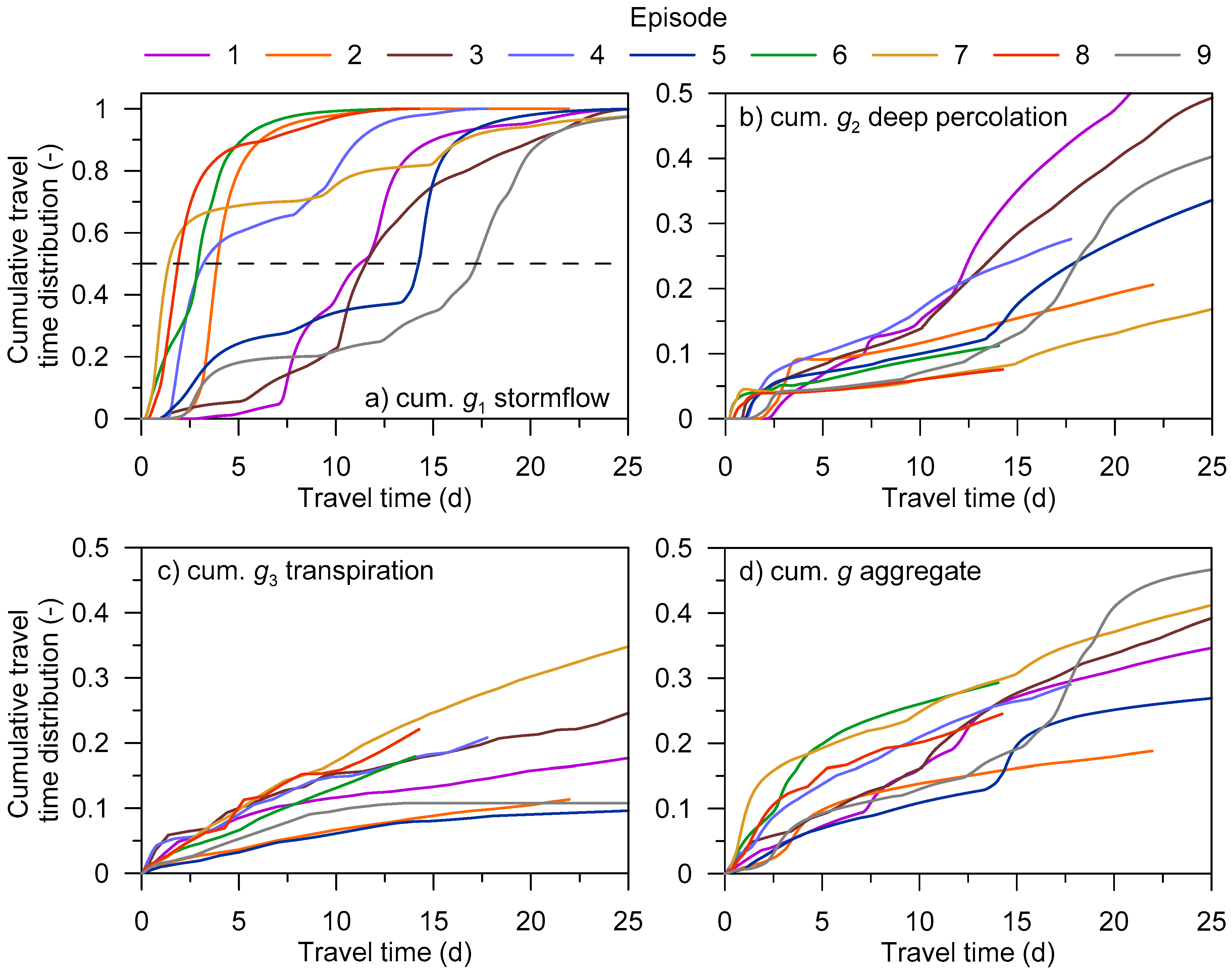
The cumulative travel time distributions of stormflow, deep percolation, and transpiration for the nine rainfall–runoff episodes are shown in Figure 4. The cumulative travel time distributions for deep percolation showed a rapid increase (within 2.5 days after the tracer application), followed by a more gradual rise for all episodes. For some episodes (Episodes 1, 3, 5, 7, and 9), the increase of the tracer mass in deep percolation was associated with the increase of the tracer mass in stormflow, especially in the second part of these episodes. Cumulative travel time distributions for deep percolation g2 were below 0.5 at the end of all episodes except for Episode 1 (Figure 4b). As expected, the cumulative travel time distributions for transpiration (g3) remained lower than 1 at the end of all episodes (Figure 4c). Unlike for stormflow and deep percolation, no significant effect of the shape of the rainfall signal occurs in the case of transpiration. The aggregate cumulative travel time distributions, combining functions g1, g2, and g3 according to Equation (4), are shown in Figure 4d. The shape of the aggregate travel time distributions indicates that the effect of episodal stormflow is less pronounced than the combined effects of the more continuous processes—deep percolation and transpiration.
Table 2 shows the median travel times tm for stormflow determined for the nine rainfall–runoff episodes. The tm values ranged from 1.4 to 17.2 days. The stormflow tm values exhibited great variability among the episodes, caused by the temporal variations of rainfall intensities as well as antecedent soil water content conditions. The tm values for transpiration and deep percolation as well as the tm values associated with the aggregate travel time distributions were not evaluated since the episodal simulations were discontinued at the end of episodes, before the cumulative travel time distribution for transpiration and deep percolation could reach the value of 0.5 (in most of the cases except g2 in Episode 1).
Table 2 reveals a number of interesting hydrological responses. For instance, Episodes 6, 7, and 8 showed very short stormflow tm values (<3 days). This was caused by the intense rainfall at the beginning of the episode, triggering the rapid initiation of both stormflow and deep percolation responses. Episode 5 was characterized by a subsurface runoff peak occurring 14 days after the tracer application, hence tm is relatively long. For five episodes (Episodes 2, 4, 6, 7, and 8), the advective component of transport dominated over the dispersive one. These episodes were characterized by rapid arrival times of the tracer to the hillslope trench, thus shorter median travel times for stormflow (<4 days). For the long-duration episodes with more complex rainfall and runoff patterns, the dispersive component caused enhanced tracer mixing in the hillslope profile leading to longer travel times.
The estimated median travel times of stormflow vary significantly among the rainfall–runoff episodes (Table 2). The highly variable relationship between hillslope storage, cumulative net input of water, and mean travel times, shown in Figure 5, suggests that the estimated tm values are strongly affected by temporal rainfall patterns and antecedent soil moisture distributions, in addition to overall hillslope storage and cumulative input of water. The episode-based stormflow tm values fell into two groups characterized by tm < 7 days and tm > 7 days. Longer values of tm were obtained for the episodes with a complex temporal rainfall distribution causing multi-peak stormflow responses. It can be seen that a greater subsurface storage is not uniquely associated with longer stormflow tm values (Figure 5).
McGuire and McDonnell [5] concluded that longer transit times indicate greater contact time and subsurface storage, implying more time for biogeochemical reactions to occur. Our results indicate that longer median travel times were associated with a wide range of hillslope water storages (Figure 5). At the catchment scale, Heidbüchel et al. [61] suggested that instead of total precipitation amount, precipitation patterns (scattered or clustered rainfall) and event intensities play a more important role influencing the magnitude of median travel times. This finding is in agreement with our results.
Besides the effect of temporal rainfall distribution, the initial hillslope storage plays an important role in the estimation of episodal tm for stormflow. Dusek and Vogel [41] demonstrated a nonlinear relationship between initial hillslope storage and stormflow. Furthermore, the initial distribution of soil water within the hillslope, specifically, the extent of soil saturation near the soil–bedrock interface, was a key factor in stormflow generation. Dusek and Vogel [41] reported that deep percolation increased with increasing initial hillslope storage. However, in the present study, highly variable tm values of stormflow were found for similar hillslope storages (Figure 5). This again signifies the importance of temporal rainfall patterns and initial soil moisture distributions.
4.2. Seasonal Soil Water Balance, Residence Times, and Travel Time Distributions
The components of hillslope water balance are shown in Table 3. It can be seen that transpiration represents about 57% of rainfall. Growing season 2009 is characterized by larger rainfall and smaller transpiration compared to seasons 2007 and 2008, resulting in greater stormflow and deep percolation volumes. Dusek and Vogel [40] reported a reasonable agreement between observed and predicted seasonal volumes of stormflow. The initial and final hillslope storages in Table 3 refer to soil water integrated over the soil layers above the soil–bedrock interface at the beginning and end of the growing seasons.
The estimated mean residence times T, defined in Equation (1), for growing seasons 2007, 2008, and 2009 were 36.8, 35.7, and 29.4 days, respectively. The residence times were calculated from the mean hillslope storages and mean hillslope discharges (stormflow, deep percolation, and transpiration combined). While stormflow is characterized by short-lived responses, deep percolation is more persistent. Shorter mean residence time for 2009 season can be explained by greater rainfall input thus larger stormflow volume than for 2007 and 2008 seasons.
Transpiration flux is often excluded from the calculation of mean residence time e.g., [5]. If done in our case, much longer residence times with amplified interannual variability would be obtained (equal to 128.1, 89.0, and 53.6 days for seasons 2007, 2008, and 2009, respectively).
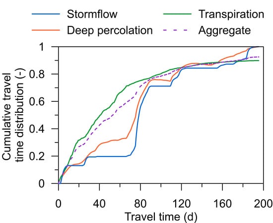
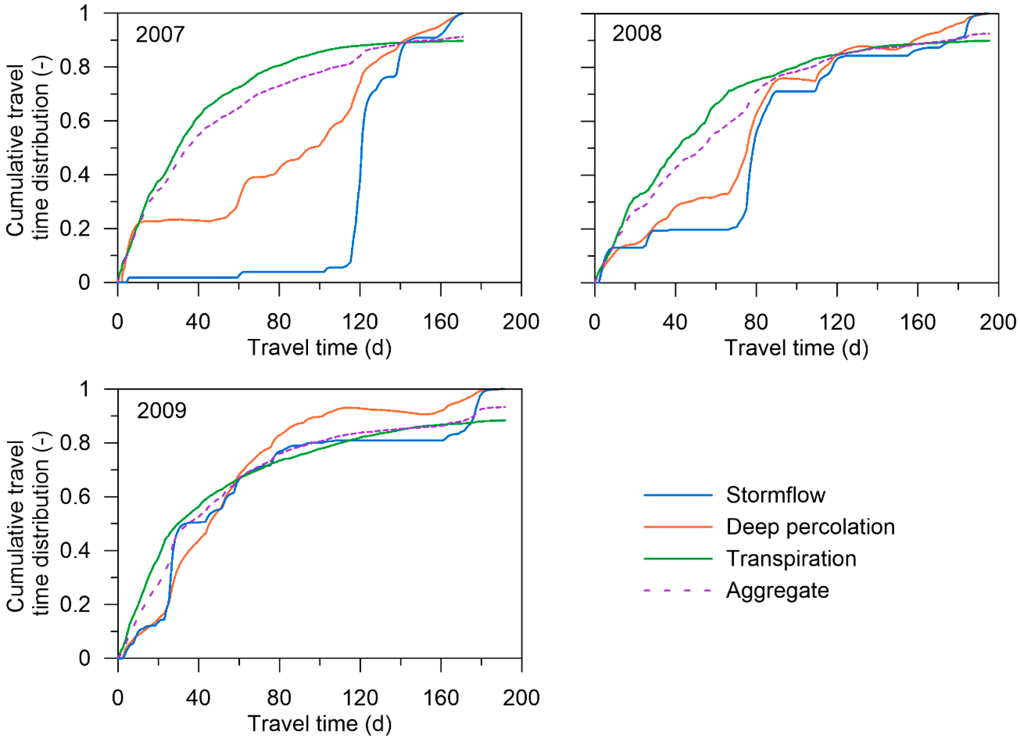
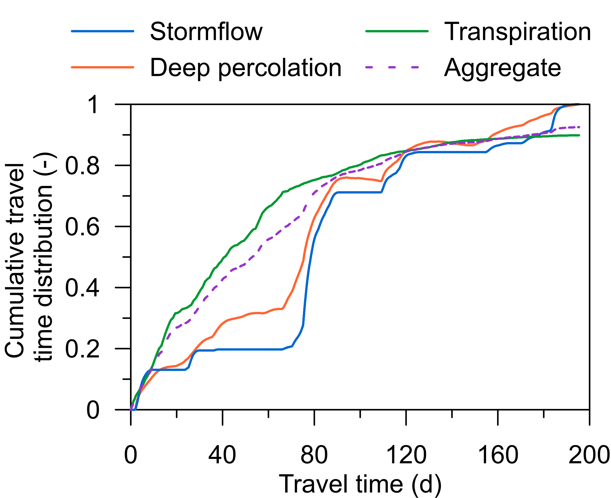
The cumulative partial travel time distributions for stormflow, transpiration, and deep percolation for growing seasons 2007–2009 are shown in Figure 6. The steep increase of cumulative travel time distribution of transpiration at the beginning of each season is related to the higher transpiration demand during summer months and the high availability of the tracer (entering the soil profile at the beginning of each season). Later, the tracer uptake by roots becomes less intense and the tracer concentration more diluted. The cumulative travel time distributions for deep percolation and stormflow are more variable from season to season reflecting different number and timing of major rainfall–runoff episodes.
Figure 6 also shows the aggregate travel time distributions (combining the effects of all hillslope discharge processes). Due to the higher relative weight of transpiration compared to stormflow and deep percolation (cf. Equation (4) and Table 4) the shape of the aggregate travel time distributions is close to that determined for transpiration.
Significantly different seasonal median travel times, tm, were found for different discharge processes (Table 5). The shortest median travel times were determined for transpiration. As expected, the stormflow tm values showed the greatest interseasonal variability compared to the other two discharge processes.
The median aggregate travel times, affected by all hillslope discharge processes, were estimated to be 30.4, 46.2, and 30.1 days for seasons 2007, 2008, and 2009, respectively (Table 5). These travel times can be directly compared with the mean residence times T estimated using Equation (1) for the three seasons (36.8, 35.7, and 29.4 days). For 2009 season, characterized by a large rainfall input, the values of tm and T are very similar. The differences between tm and T values for the drier seasons 2007 and 2008 are greater.
Despite the fact that transpiration constitutes a significant part of soil water balance, its role is rarely explicitly accounted for in the estimation of median hillslope travel times. The effect of transpiration is lumped when convolution-based approaches are applied. Sprenger et al. [62] found significantly shorter median travel times for transpiration during spring and summer (30–41 days) compared with events occurring during fall and winter (130 days). In our study, the estimated median travel times for transpiration were between 24 and 35 days for the growing seasons considered (Table 5), with spring period characterized by enhanced atmospheric demands.
4.3. Tracer Mass Partitioning
The respective fractions of the total tracer mass, applied at the beginning of the rainfall–runoff episodes, discharged by stormflow, deep percolation, and transpiration are shown in Table 6. These fractions reflect the relative importance of individual processes contributing to the overall hillslope discharge. The table shows that 7–33% of the tracer mass was discharged by hillslope stormflow, 4–21% left the hillslope soil profile via transpiration, and 3–12% leaked into the deeper weathered bedrock (passing through the soil–bedrock interface). Most of the applied tracer (52–81%) remained in the hillslope soil (above the soil–bedrock interface). As expected, the residual amount of tracer in the soil at the end of each episode is inversely proportional to the net water input during the episode.
The residual tracer mass fractions in seasonal simulations (Table 4) were much lower compared to episodal simulations. Tracer mass remaining in the hillslope soil at the end of the growing season ranged from 7 to 9% of mass applied at the beginning of the season. The largest discharge of the tracer mass was associated with transpiration, ranging between 51 and 76%. Tracer masses associated with stormflow were between 5 and 24%. The mass fractions in deep percolation ranged from 10 to 19% of the applied mass.
5. Summary and Conclusions
A two-dimensional dual-continuum model was used to evaluate the travel time distributions of water through a forest hillslope exhibiting significant lateral preferential flow effects. The breakthroughs of a fictious tracer, entering the soil profile in the form of the Dirac impulse, were analyzed and the associated travel time distributions were estimated at both episodal and seasonal time scales. The modeling approach applied allowed us to evaluate the partial travel time distributions for the relevant hillslope discharge processes, namely subsurface stormflow, deep percolation and transpiration as well as the aggregate travel time distributions characterizing the combination of all discharge processes. The numerical experiments were performed for three growing seasons and major rainfall–runoff episodes. The episodes differed in temporal rainfall patterns and initial distributions of soil water within the hillslope.
The obtained episodal travel time distributions suggest a quick hydrological response of the hillslope to rainfall, which can be attributed to the inclusion of preferential flow component in the model. The variability of the travel time distributions was found to be controlled by the meteorological conditions during the rainfall–runoff episodes and antecedent soil moisture distribution prior to the episodes. The flow-corrected time projection allowed as to construct master travel time distribution for stormflow, which can be used to compare the hydrological response of the hillslope of interest with that of other hillslopes.
The episodal median travel times of subsurface stormflow ranged from 1 to 17 days for the selected rainfall–runoff episodes. The results indicated a weak relationship between stormflow travel times and hillslope water storages. The seasonal aggregate median travel time (for all discharge processes combined) was estimated in the range of 30–46 days.
Transpiration was shown to have significant impact on the estimated seasonal as well as episodal aggregate travel time distributions. Transpiration had to be also considered in the calculations of mean residence times as it represents a significant part of the water balance. The mean residence times ranged between 29 and 37 days for the three seasons considered.
Once validated on experimental observations, the numerical model offers a valuable tool for the evaluation of soil water travel times in hillslopes. For instance, the flux partitioning in the subsurface, reflected in median travel times of the different discharge processes, may be used for the quantification of biogeochemical transformations of dissolved organic compounds. The partial travel time distributions associated with the different discharge mechanisms provide meaningful information for the catchment runoff modeling.
Author Contributions
Both authors were responsible for the study conceptualization, writing, and editing. Both authors reviewed and contributed to the final manuscript.
Funding
This study was supported by the Czech Science Foundation, project No. 17-00630J.
Acknowledgments
The authors wish to thank the Supercomputing Center of the CTU in Prague for the possibility of running the 2D simulations on its computer network.
Conflicts of Interest
The authors declare no conflict of interest.
References
- Danesh-Yazdi, M.; Klaus, J.; Condon, L.E.; Maxwell, R.M. Bridging the gap between numerical solutions of travel time distributions and analytical storage selection functions. Hydrol. Process. 2018, 32, 1063–1076. [Google Scholar] [CrossRef]
- Woods, R.; Rowe, L. The changing spatial variability of subsurface flow across a hillside. J. Hydrol. 1996, 5, 51–86. [Google Scholar]
- Weiler, M.; McDonnell, J.J.; Tromp-van Meerveld, I.; Uchida, T. Subsurface stormflow. In Encyclopedia of Hydrological Sciences; Anderson, M.G., Ed.; John Wiley & Sons: New York, NY, USA, 2005. [Google Scholar]
- Bachmair, S.; Weiler, M. Interactions and connectivity between runoff generation processes of different spatial scales. Hydrol. Process. 2014, 28, 1916–1930. [Google Scholar] [CrossRef]
- McGuire, K.J.; McDonnell, J.J. A review and evaluation of catchment transit time modeling. J. Hydrol. 2006, 330, 543–563. [Google Scholar] [CrossRef]
- Rodhe, H. Modeling biogeochemical cycles. In Earth System Science; Elsevier Academic Press: London, UK, 2000; pp. 62–84. [Google Scholar]
- Asano, Y.; Uchida, T.; Ohte, N. Residence times and flow paths of water in steep unchannelled catchments, Tanakami, Japan. J. Hydrol. 2002, 261, 173–192. [Google Scholar] [CrossRef]
- Kabeya, N.; Shimizu, A.; Tamai, K.; Iida, S.; Shimizu, T. Transit times of soil water in thick soil and weathered gneiss layers using deuterium excess modelling. In Conceptual and Modelling Studies of Integrated Groundwater, Surface Water, and Ecological Systems (IAHS Publ. 345); Abesser, C., Naütman, G., Hill, M.C., Blöshl, G., Laksmanan, E., Eds.; IAHS Press: Wallingford, UK, 2011; pp. 163–168. [Google Scholar]
- Kim, S.; Jung, S. Estimation of mean water transit time on a steep hillslope in South Korea using soil moisture measurements and deuterium excess. Hydrol. Process. 2014, 28, 1844–1857. [Google Scholar] [CrossRef]
- Onderka, M.; Chudoba, V. The Wavelets show it—The transit time of water varies in time. J. Hydrol. Hydromech. 2018, 66, 295–302. [Google Scholar] [CrossRef]
- McGuire, K.J.; McDonnell, J.J.; Weiler, M.; Kendall, C.; McGlynn, B.L.; Welker, J.M.; Seibert, J. The role of topography on catchment-scale water residence time. Water Resour. Res. 2005, 41, W05002. [Google Scholar] [CrossRef]
- Stewart, M.K.; McDonnell, J.J. Modeling base-flow soil-water residence times from deuterium concentrations. Water Resour. Res. 1991, 27, 2681–2693. [Google Scholar] [CrossRef]
- Kabeya, N.; Katsuyama, M.; Kawasaki, M.; Ohte, N.; Sugimoto, A. Estimation of mean residence times of subsurface waters using seasonal variation in deuterium excess in a small headwater catchment in Japan. Hydrol. Process. 2007, 21, 308–322. [Google Scholar] [CrossRef]
- Vitvar, T.; Balderer, W. Estimation of mean water residence times and runoff generation by180 measurements in a Pre-Alpine catchment (Rietholzbach, Eastern Switzerland). Appl. Geochem. 1997, 12, 787–796. [Google Scholar] [CrossRef]
- Matsutani, J.; Tanaka, T.; Tsujimura, M. Residence times of soil, ground, and discharge waters in a mountainous headwater basin, central Japan, traced by tritium. In Tracers in Hydrology; International Association for Hydrological Science: Yokohama, Japan, 1993; pp. 57–63. [Google Scholar]
- Sprenger, M.; Stumpp, C.; Weiler, M.; Aeschbach, W.; Allen, S.T.; Benettin, P.; McDonnell, J.J. The demographics of water: A review of water ages in the critical zone. Rev. Geophys. 2019, 57, 800–834. [Google Scholar] [CrossRef]
- Hrachowitz, M.; Benettin, P.; van Breukelen, B.M.; Fovet, O.; Howden, N.J.; Ruiz, L.; Wade, A.J. Transit times—The link between hydrology and water quality at the catchment scale. WIREs Water 2016, 3, 629–657. [Google Scholar] [CrossRef]
- Botter, G.; Bertuzzo, E.; Rinaldo, A. Catchment residence and travel time distributions: The master equation. Geophys. Res. Lett. 2011, 38, L11403. [Google Scholar] [CrossRef]
- McGuire, K.J.; Weiler, M.; McDonnell, J.J. Integrating tracer experiments with modeling to assess runoff processes and water transit times. Adv. Water Resour. 2007, 30, 824–837. [Google Scholar] [CrossRef]
- Rodhe, A.; Nyberg, L.; Bishop, K. Transit times for water in a small till catchment from a step shift in the Oxygen 18 content of the water input. Water Resour. Res. 1996, 32, 3497–3511. [Google Scholar] [CrossRef]
- Maloszewski, P.; Zuber, A. Determining the turnover time of groundwater systems with the aid of environmental tracers: 1. Models and their applicability. J. Hydrol. 1982, 57, 207–231. [Google Scholar] [CrossRef]
- Tetzlaff, D.; Malcolm, I.A.; Soulsby, C. Influence of forestry, environmental change and climatic variability on the hydrology, hydrochemistry and residence times of upland catchments. J. Hydrol. 2007, 346, 93–111. [Google Scholar] [CrossRef]
- Stumpp, C.; Maloszewski, P. Quantification of preferential flow and flow heterogeneities in an unsaturated soil planted with different crops using the environmental isotope δ18O. J. Hydrol. 2010, 394, 407–415. [Google Scholar] [CrossRef]
- Sanda, M.; Vitvar, T.; Kulasova, A.; Jankovec, J.; Cislerova, M. Run-off formation in a humid, temperate headwater catchment using a combined hydrological, hydrochemical and isotopic approach (Jizera Mountains, Czech Republic). Hydrol. Process. 2014, 28, 3217–3229. [Google Scholar] [CrossRef]
- Vogel, T.; Sanda, M.; Dusek, J.; Dohnal, M.; Votrubova, J. Using oxygen-18 to study the role of preferential flow in the formation of hillslope runoff. Vadose Zone J. 2010, 9, 252–259. [Google Scholar] [CrossRef]
- Klaus, J.; Chun, K.P.; McGuire, K.J.; McDonnell, J.J. Temporal dynamics of catchment transit times from stable isotope data. Water Resour. Res. 2015, 51, 4208–4223. [Google Scholar] [CrossRef]
- Rinaldo, A.; Benettin, P.; Harman, C.; Hrachowitz, M.; McGuire, K.; van der Velde, Z.; Bertuzzo, E.; Botter, G. Storage selection functions: A coherent framework for quantifying how catchments store and release water and solutes. Water Resour. Res. 2015, 51, 4840–4847. [Google Scholar] [CrossRef]
- van der Velde, Y.; Heidbüchel, I.; Lyon, S.W.; Nyberg, L.; Rodhe, A.; Bishop, K.; Troch, P.A. Consequences of mixing assumptions for time-variable travel time distributions. Hydrol. Process. 2015, 29, 3460–3474. [Google Scholar] [CrossRef]
- Benettin, P.; Soulsby, C.; Birkel, C.; Tetzlaff, D.; Botter, G.; Rinaldo, A. Using SAS functions and high-resolution isotope data to unravel travel time distributions in headwater catchments. Water Resour. Res. 2017, 53, 1864–1878. [Google Scholar] [CrossRef]
- Cardenas, M.B.; Jiang, X.-W. Groundwater flow, transport, and residence times through topography-driven basins with exponentially decreasing permeability and porosity. Water Resour. Res. 2010, 46, W11538. [Google Scholar] [CrossRef]
- Molénat, J.; Gascuel-Odoux, C.; Aquilina, L.; Ruiz, L. Use of gaseous tracers (CFCs and SF6) and transit-time distribution spectrum to validate a shallow groundwater transport model. J. Hydrol. 2013, 480, 1–9. [Google Scholar] [CrossRef]
- Heße, F.; Zink, M.; Kumar, R.; Samaniego, L.; Attinger, S. Spatially distributed characterization of soil-moisture dynamics using travel-time distributions. Hydrol. Earth Syst. Sci. 2017, 21, 549–570. [Google Scholar] [CrossRef]
- Kuppel, S.; Tetzlaff, D.; Maneta, M.P.; Soulsby, C. EcH2O-iso 1.0: Water isotopes and age tracking in a process-based, distributed ecohydrological model. Geosci. Model Dev. 2018, 11, 3045–3069. [Google Scholar] [CrossRef]
- Fiori, A.; Russo, D. Travel time distribution in a hillslope: Insight from numerical simulations. Water Resour. Res. 2008, 44, W12426. [Google Scholar] [CrossRef]
- Remondi, F.; Botter, M.; Burlando, P.; Fatichi, S. Variability of transit time distributions with climate and topography: A modelling approach. J. Hydrol. 2019, 569, 37–50. [Google Scholar] [CrossRef]
- Ameli, A.A.; Amvrosiadi, N.; Grabs, T.; Laudon, H.; Creed, I.F.; McDonnell, J.J.; Bishop, K. Hillslope permeability architecture controls on subsurface transit time distribution and flow paths. J. Hydrol. 2016, 543, 17–30. [Google Scholar] [CrossRef]
- Vanderborght, J.; Vereecken, H. Review of dispersivities for transport modeling in soils. Vadose Zone J. 2007, 6, 29–52. [Google Scholar] [CrossRef]
- Klaus, J.; McDonnell, J.J. Hydrograph separation using stable isotopes: Review and evaluation. J. Hydrol. 2013, 505, 47–64. [Google Scholar] [CrossRef]
- Larsbo, M. An episodic transit time model for quantification of preferential solute transport. Vadose Zone J. 2011, 10, 378–385. [Google Scholar] [CrossRef]
- Dusek, J.; Vogel, T. Modeling subsurface hillslope runoff dominated by preferential flow: One-vs. two-dimensional approximation. Vadose Zone J. 2014, 13. [Google Scholar] [CrossRef]
- Dusek, J.; Vogel, T. Hillslope-storage and rainfall-amount thresholds as controls of preferential stormflow. J. Hydrol. 2016, 534, 590–605. [Google Scholar] [CrossRef]
- Dusek, J.; Vogel, T. Hillslope hydrograph separation: The effects of variable isotopic signatures and hydrodynamic mixing in macroporous soil. J. Hydrol. 2018, 563, 446–459. [Google Scholar] [CrossRef]
- Sanda, M.; Cislerova, M. Transforming hydrographs in the hillslope subsurface. J. Hydrol. Hydromech. 2009, 57, 264–275. [Google Scholar] [CrossRef]
- Dohnal, M.; Dusek, J.; Vogel, T. The impact of the retention curve hysteresis on prediction of soil water dynamics. J. Hydrol. Hydromech. 2006, 54, 258–268. [Google Scholar]
- Dohnal, M.; Dusek, J.; Vogel, T.; Herza, J.; Tacheci, P. Analysis of soil water response to grass transpiration. Soil Water Res. 2006, 1, 85–98. [Google Scholar]
- Chow, V.T.; Maidment, D.R.; Mays, L.W. Applied Hydrology; McGraw-Hill Book Co.: Singapore, 1988. [Google Scholar]
- Zuber, A. On the interpretation of tracer data in variable flow systems. J. Hydrol. 1986, 86, 45–57. [Google Scholar] [CrossRef]
- Heidbüchel, I.; Troch, P.A.; Lyon, S.W.; Weiler, M. The master transit time distribution of variable flow systems. Water Resour. Res. 2012, 48, W06520. [Google Scholar] [CrossRef] [Green Version]
- Vogel, T.; Gerke, H.H.; Zhang, R.; van Genuchten, M.T. Modeling flow and transport in a two-dimensional dual-permeability system with spatially variable hydraulic properties. J. Hydrol. 2000, 238, 78–89. [Google Scholar] [CrossRef]
- Gerke, H.H.; van Genuchten, M.T. A dual-porosity model for simulating the preferential movement of water and solutes in structured porous media. Water Resour. Res. 1993, 29, 305–319. [Google Scholar] [CrossRef]
- Bear, J. Dynamics of Fluids in Porous Materials; Elsevier: New York, NY, USA, 1972. [Google Scholar]
- Gerke, H.H.; Dusek, J.; Vogel, T.; Köhne, J.M. Two-dimensional dual permeability analyses of a bromide tracer experiment on a tile-drained field. Vadose Zone J. 2007, 6, 651–667. [Google Scholar] [CrossRef]
- Dusek, J.; Gerke, H.H.; Vogel, T. Surface boundary conditions in two-dimensional dual-permeability modeling of tile drain bromide leaching. Vadose Zone J. 2008, 7, 1287–1301. [Google Scholar] [CrossRef]
- Monteith, J.L. Evaporation and surface temperature. Q. J. R. Meteorol. Soc. 1981, 107, 1–27. [Google Scholar] [CrossRef]
- Feddes, R.A.; Kowalik, P.J.; Zaradny, H. Simulation of Field Water use and Crop Yield; Simul. Monogr., Cent. for Agric. Publ. and Doc.: Wageningen, The Netherlands, 1978; p. 189. [Google Scholar]
- Van Genuchten, M.T. A closed-form equation for predicting the hydraulic conductivity of unsaturated soils. Soil Sci. Soc. Am. J. 1980, 44, 892–898. [Google Scholar] [CrossRef] [Green Version]
- Vogel, T.; Cislerova, M. On the reliability of unsaturated hydraulic conductivity calculated from the moisture retention curve. Transp. Porous Media 1988, 3, 1–15. [Google Scholar] [CrossRef]
- Vogel, T.; van Genuchten, M.T.; Cislerova, M. Effect of the shape of soil hydraulic properties near saturation on numerical simulation of variably-saturated flow. Adv. Water Resour. 2000, 24, 133–144. [Google Scholar] [CrossRef]
- Dusek, J.; Vogel, T.; Dohnal, M.; Gerke, H.H. Combining dual-continuum approach with diffusion wave model to include a preferential flow component in hillslope scale modeling of shallow subsurface runoff. Adv. Water Resour. 2012, 44, 113–125. [Google Scholar] [CrossRef]
- Dusek, J.; Vogel, T.; Sanda, M. Hillslope hydrograph analysis using synthetic and natural oxygen-18 signatures. J. Hydrol. 2012, 475, 415–427. [Google Scholar] [CrossRef]
- Heidbüchel, I.; Troch, P.A.; Lyon, S.W. Separating physical and meteorological controls of variable transit times in zero-order catchments. Water Resour. Res. 2013, 49, 7644–7657. [Google Scholar] [CrossRef]
- Sprenger, M.; Seeger, S.; Blume, T.; Weiler, M. Travel times in the vadose zone: Variability in space and time. Water Resour. Res. 2016, 52, 5727–5754. [Google Scholar] [CrossRef] [Green Version]
Figure 1.
Two-dimensional flow domain representing the hillslope segment at the Tomsovka experimental site: (a) schematics of the hillslope segment with the experimental trench for collecting subsurface hillslope discharge (b) flow domain with the detail of the subsurface trench.
Figure 1.
Two-dimensional flow domain representing the hillslope segment at the Tomsovka experimental site: (a) schematics of the hillslope segment with the experimental trench for collecting subsurface hillslope discharge (b) flow domain with the detail of the subsurface trench.
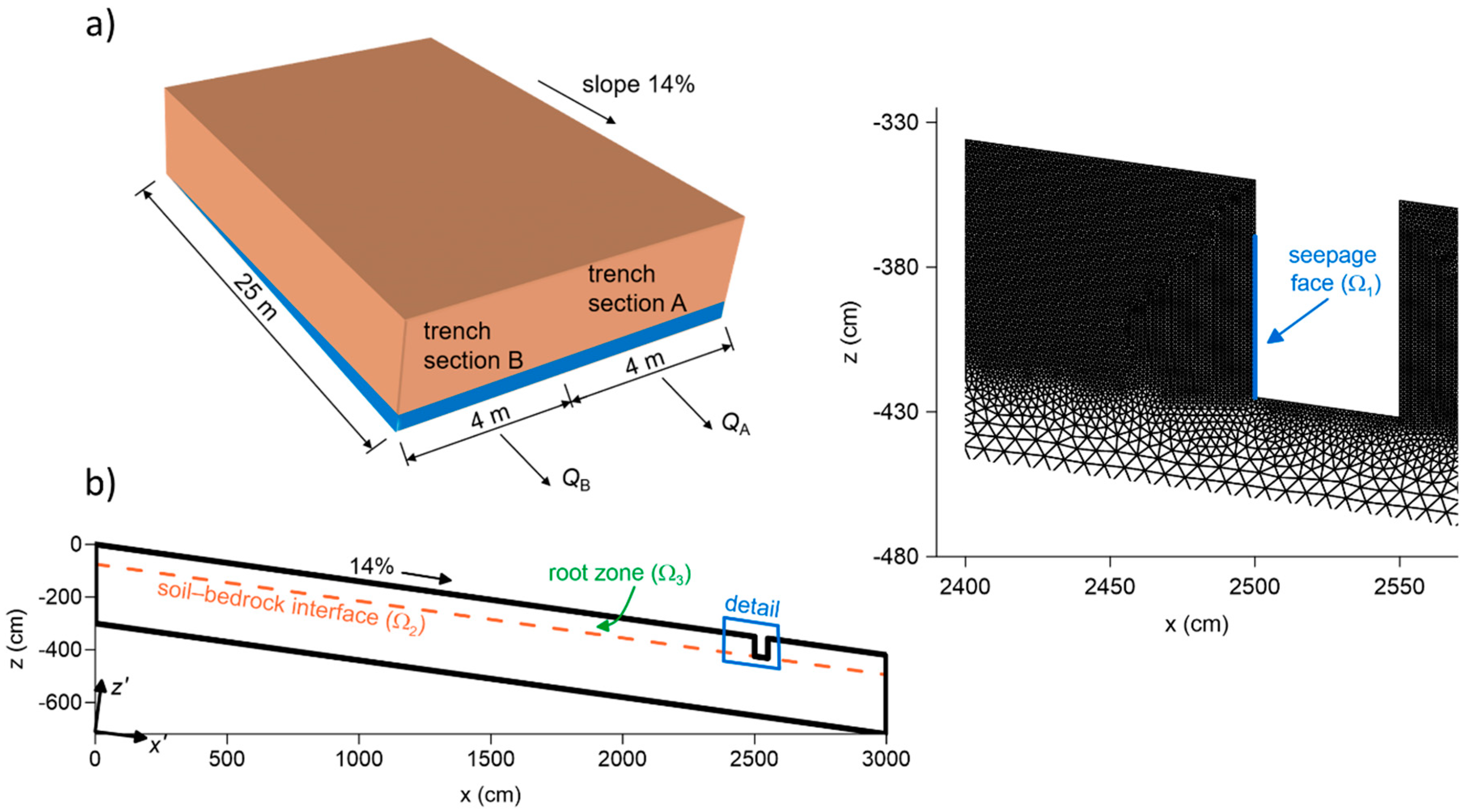
Figure 2.
Observed (trench sections A and B) and simulated hillslope discharge hydrographs during selected rainfall–runoff episodes recorded over the period of three years. The rainfall–runoff episodes are marked with numbers. Adopted from Dusek and Vogel [42].
Figure 2.
Observed (trench sections A and B) and simulated hillslope discharge hydrographs during selected rainfall–runoff episodes recorded over the period of three years. The rainfall–runoff episodes are marked with numbers. Adopted from Dusek and Vogel [42].
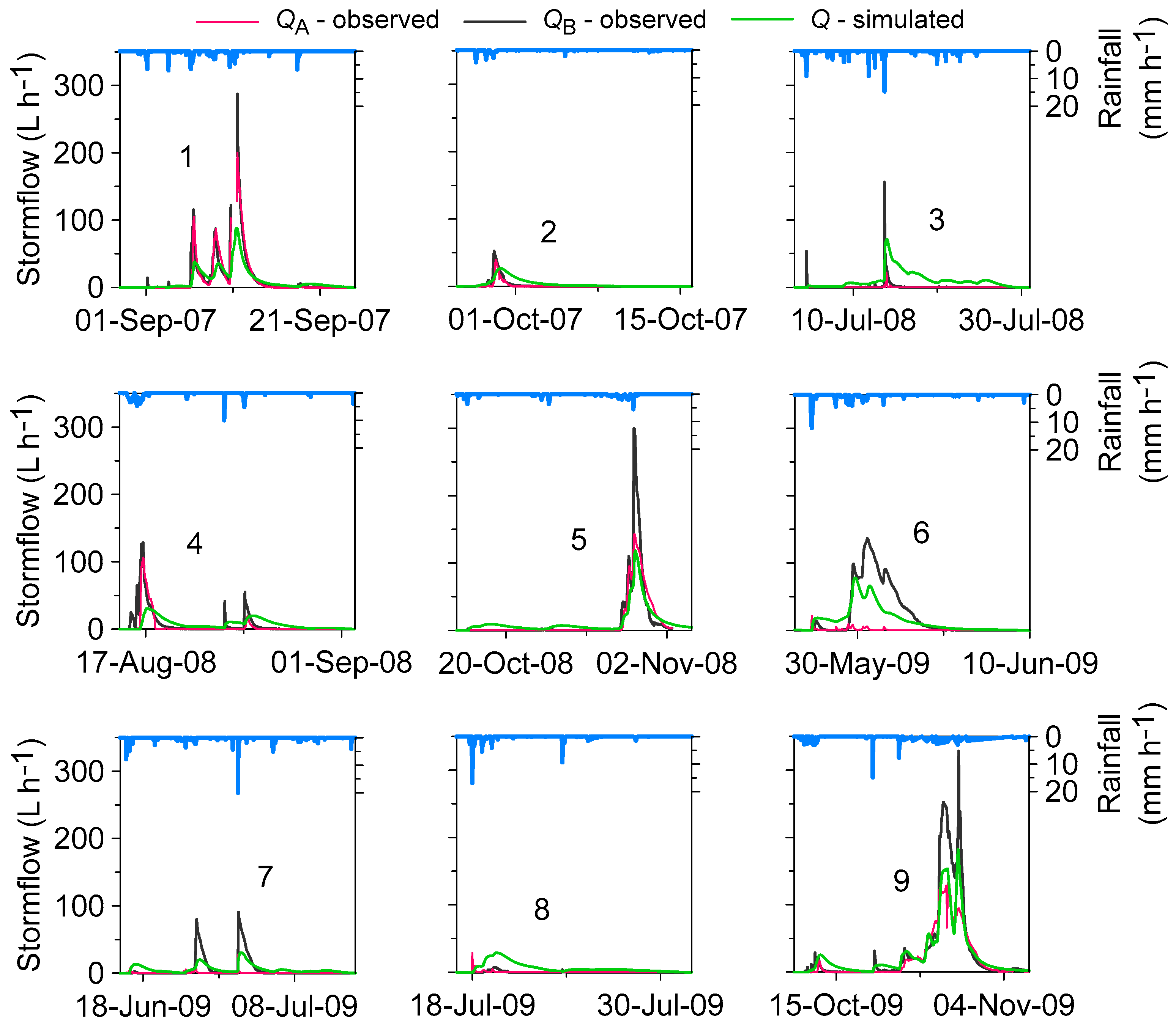
Figure 3.
Episodal travel time distributions of stormflow for the selected rainfall–runoff episodes plotted against travel time since tracer application (a) and against flow-corrected travel time obtained as the cumulative volume of stormflow divided by the final volume of rainfall (b). The master travel time distribution is shown in the flow-corrected time projection.
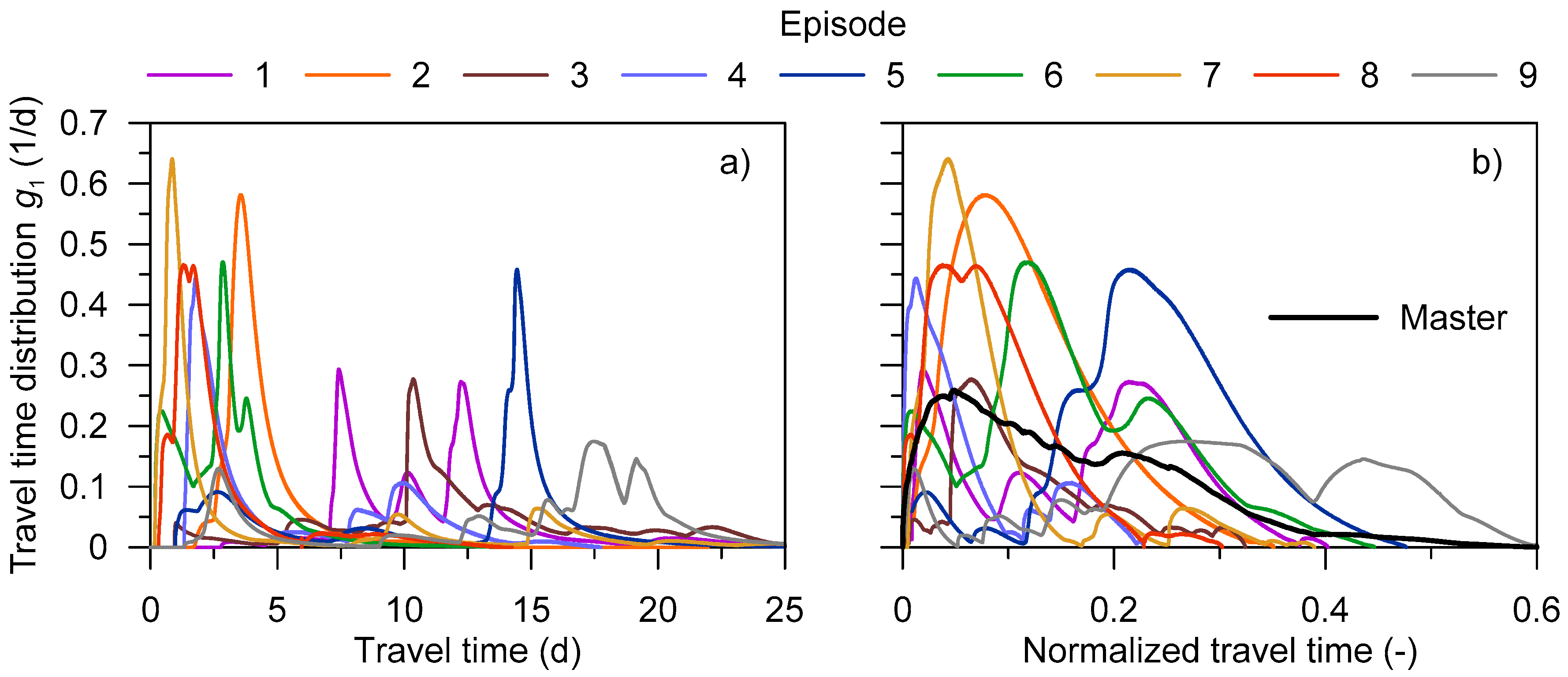
Figure 4.
Cumulative travel time distributions of stormflow (a), deep percolation (b), and transpiration (c), as well as aggregate distributions combing all discharge processes (d) for the selected rainfall–runoff episodes. Median travel times tm for stormflow correspond to the value of cumulative travel time distribution equal to 0.5.

Figure 5.
The relationships between net water input (rainfall minus transpiration), hillslope storage and stormflow median travel times, tm, for the selected rainfall–runoff episodes. The circles are labeled with the episode numbers. The magnitude of the respective median travel time (cf. Table 2) is expressed by the circle diameter.
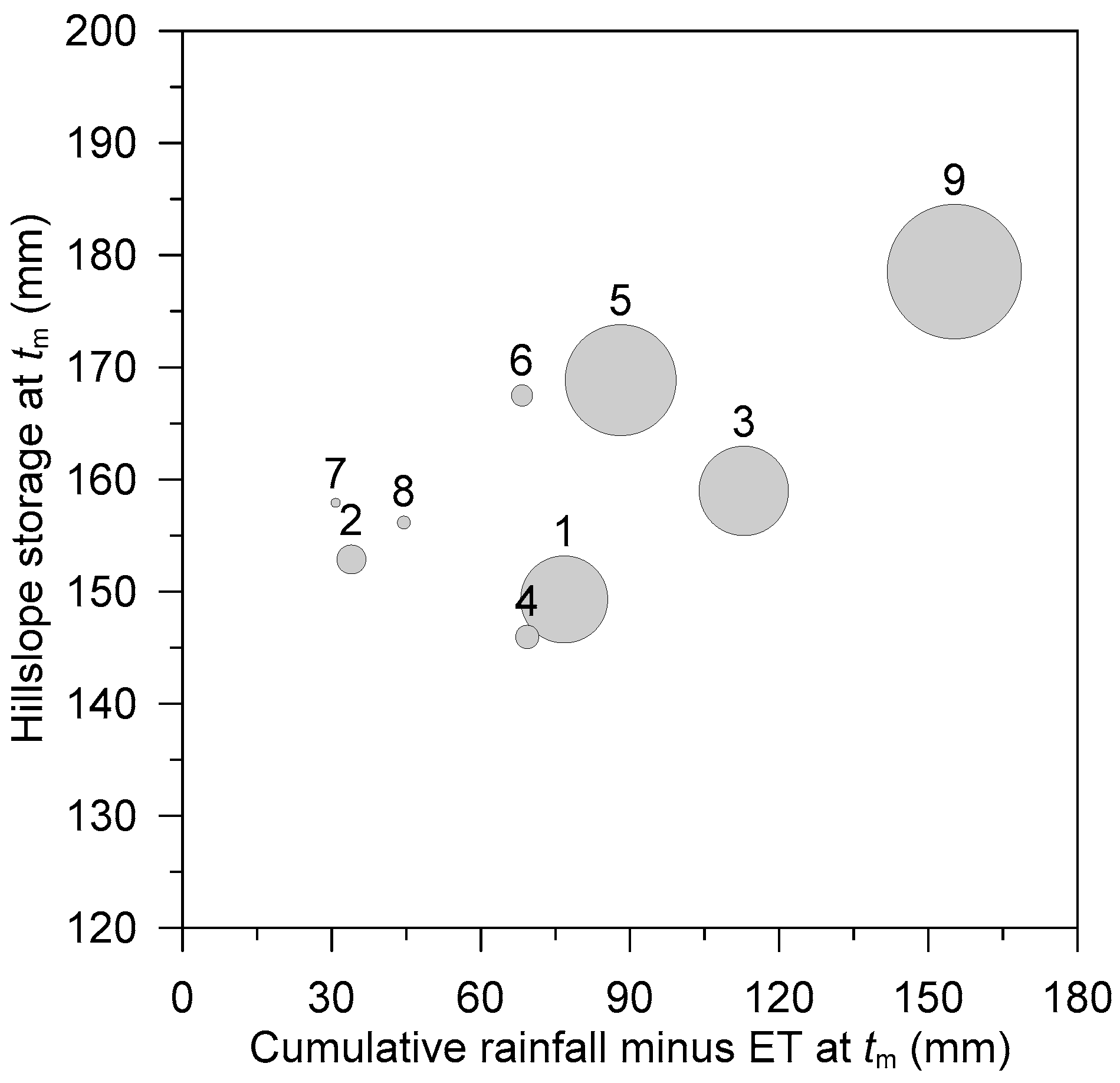
Figure 6.
Cumulative travel time distributions of stormflow, deep percolation and transpiration, together with the aggregate travel time distributions for growing seasons 2007, 2008, and 2009.
Figure 6.
Cumulative travel time distributions of stormflow, deep percolation and transpiration, together with the aggregate travel time distributions for growing seasons 2007, 2008, and 2009.

Table 1.
The soil hydraulic parameters † used for the two-dimensional dual-continuum model. SM and PF refer to the soil matrix and preferential flow domain, respectively.
Table 1.
The soil hydraulic parameters † used for the two-dimensional dual-continuum model. SM and PF refer to the soil matrix and preferential flow domain, respectively.
| Depth | θr | θs | α | n | Ks | hs | |
|---|---|---|---|---|---|---|---|
| (cm) | (cm3 cm−3) | (cm3 cm−3) | (cm−1) | (-) | (cm d−1) | (cm) | |
| SM | 0–8 | 0.20 | 0.55 | 0.050 | 2.00 | 567 | 0.00 |
| 8–20 | 0.20 | 0.54 | 0.050 | 1.50 | 67 | −0.69 | |
| 20–70 | 0.20 | 0.49 | 0.020 | 1.20 | 17 | −1.48 | |
| 70–75 | 0.20 | 0.41 | 0.020 | 1.20 | 1.3 | −1.88 | |
| 75–300 | 0.00 | 0.21 | 0.020 | 1.20 | 0.4 | −2.61 | |
| PF | 0–70 | 0.01 | 0.60 | 0.050 | 3.00 | 5000 | 0.00 |
| 70–300 | 0.01 | 0.60 | 0.050 | 3.00 | 0.4 | 0.00 |
† θr and θs are the residual and saturated water contents, Ks is the vertical saturated hydraulic conductivity, hs is the air-entry value, and α and n are empirical fitting parameters.
Table 2.
Estimated median travel times tm of stormflow determined for the selected rainfall–runoff episodes.
Table 2.
Estimated median travel times tm of stormflow determined for the selected rainfall–runoff episodes.
| Episode | 1 | 2 | 3 | 4 | 5 | 6 | 7 | 8 | 9 |
| Episode Duration (d) | 27 | 22 | 26 | 18 | 26 | 14 | 32 | 14 | 33 |
| tm (d) | 11.2 | 3.9 | 11.5 | 3.2 | 14.2 | 2.9 | 1.4 | 1.9 | 17.2 |
Table 3.
Simulated components of the hillslope soil water balance.
| Season | 2007 | 2008 | 2009 |
| Season Duration (d) | 171 | 191 | 191 |
| Observed Rainfall (mm) | 634 | 724 | 874 |
| Stormflow (mm) | 97 | 169 | 301 |
| Deep Percolation (mm) | 76 | 125 | 182 |
| Transpiration (mm) | 429 | 438 | 396 |
| Initial Storage (mm) | 106 | 145 | 145 |
| Final Storage (mm) | 138 | 137 | 140 |
Table 4.
Mass fractions of tracer relative to applied mass. Net water input is rainfall minus actual transpiration.
Table 4.
Mass fractions of tracer relative to applied mass. Net water input is rainfall minus actual transpiration.
| Season | 2007 | 2008 | 2009 |
| Net Water Input (mm) | 205 | 286 | 478 |
| Stormflow (%) | 5.0 | 12.8 | 23.5 |
| Deep Percolation (%) | 9.9 | 13.5 | 18.8 |
| Transpiration (%) | 76.3 | 66.2 | 51.0 |
| Residual (%) | 8.8 | 7.5 | 6.7 |
Table 5.
Median travel times.
| Season | 2007 | 2008 | 2009 |
| Stormflow (d) | 120.9 | 78.5 | 33.5 |
| Deep Percolation (d) | 95.8 | 75.5 | 35.4 |
| Transpiration (d) | 26.4 | 35.4 | 23.5 |
| Aggregate (d) | 30.4 | 46.2 | 30.1 |
Table 6.
Mass fractions of tracer relative to applied mass at the end of rainfall–runoff episodes. Net water input is rainfall minus actual transpiration.
Table 6.
Mass fractions of tracer relative to applied mass at the end of rainfall–runoff episodes. Net water input is rainfall minus actual transpiration.
| Episode | 1 | 2 | 3 | 4 | 5 | 6 | 7 | 8 | 9 |
| Net Water Input (mm) | 121 | 28 | 130 | 91 | 102 | 80 | 77 | 36 | 260 |
| Stormflow (%) | 14.9 | 7.2 | 13.6 | 8.7 | 14.5 | 16.4 | 18.8 | 9.4 | 32.5 |
| Deep Percolation (%) | 7.0 | 2.5 | 8.9 | 5.1 | 6.0 | 3.5 | 6.3 | 2.5 | 11.6 |
| Transpiration (%) | 13.7 | 9.2 | 18.0 | 15.1 | 6.6 | 9.4 | 21.0 | 12.6 | 4.4 |
| Residual (%) | 64.4 | 81.2 | 59.5 | 71.0 | 72.8 | 70.7 | 53.9 | 75.5 | 51.5 |
© 2019 by the authors. Licensee MDPI, Basel, Switzerland. This article is an open access article distributed under the terms and conditions of the Creative Commons Attribution (CC BY) license (http://creativecommons.org/licenses/by/4.0/).
Share and Cite
MDPI and ACS Style
Dusek, J.; Vogel, T. Modeling Travel Time Distributions of Preferential Subsurface Runoff, Deep Percolation and Transpiration at A Montane Forest Hillslope Site. Water 2019, 11, 2396. https://doi.org/10.3390/w11112396
AMA Style
Dusek J, Vogel T. Modeling Travel Time Distributions of Preferential Subsurface Runoff, Deep Percolation and Transpiration at A Montane Forest Hillslope Site. Water. 2019; 11(11):2396. https://doi.org/10.3390/w11112396
Chicago/Turabian StyleDusek, Jaromir, and Tomas Vogel. 2019. "Modeling Travel Time Distributions of Preferential Subsurface Runoff, Deep Percolation and Transpiration at A Montane Forest Hillslope Site" Water 11, no. 11: 2396. https://doi.org/10.3390/w11112396
Note that from the first issue of 2016, this journal uses article numbers instead of page numbers. See further details here.