Modelling the Effects of Historical and Future Land Cover Changes on the Hydrology of an Amazonian Basin

Abstract

Land cover changes (LCC) affect the water balance (WB), changing surface runoff (SurfQ), evapotranspiration (ET), groundwater (GW) regimes, and streamflow (Q). The Tapajós Basin (southeastern Amazon) has experienced LCC over the last 40 years, with increasing LCC rates projected for the near future. Several studies have addressed the effects of climate changes on the region’s hydrology, but few have explored the effects of LCC on its hydrological regime. In this study, the Soil and Water Assessment Tool (SWAT) was applied to model the LCC effects on the hydrology of the Upper Crepori River Basin (medium Tapajós Basin), using historical and projected LCC based on conservation policies (GOV_2050) and on the “Business as Usual” trend (BAU_2050). LCC that occurred from 1973 to 2012, increased Q by 2.5%, without noticeably altering the average annual WB. The future GOV_2050 and BAU_2050 scenarios increased SurfQ by 238.87% and 300.90%, and Q by 2.53% and 2.97%, respectively, and reduced GW by 4.00% and 5.21%, and ET by 2.07% and 2.43%, respectively. Results suggest that the increase in deforestation will intensify floods and low-flow events, and that the conservation policies considered in the GOV_2050 scenario may still compromise the region’s hydrology at a comparable level to that of the BAU_2050.

1. Introduction

Over the last four decades, the Brazilian Amazonian ecosystem has been impacted by logging, pasture ranching, mining, expansion of the road network, and agricultural exploration [1,2,3]. Although the deforestation rates of large areas have declined over recent years, small-scale clearings have increased by 34% in a recent 14 year period, representing new challenges for forest conservation [4]. In the Tapajós Basin (southeastern Amazon), these small-scale clearings are associated with small-scale gold mining activities, which also compromise the water quality in the river [5,6]. Furthermore, the water resources of important Amazonian basins, such as Madeira’s, Xingu’s, and Tapajós River Basins, are also threatened by both built and planned dams, and by increasing mining activities [7,8]. Specifically, in the Tapajós River Basin, existing and planned dams may affect the quality and quantity of water resources, in addition to flooding indigenous lands and conservation areas, thus, making this region a focal point for research on the impacts of river damming and land cover change (LCC) on the local hydrology [8].

Other studies in the Amazon have demonstrated the impacts of LCC on several aspects of the ecosystem, such as water quality [9,10], biodiversity [11,12], habitat fragmentation [13,14], and hydrology [15,16,17]. On the effects of LCC on the hydrology, for instance, Dos Santos et al. [15] state that, in the Xingu River Basin, the conversion of 57% of forest areas into pasture would increase annual streamflow by 6.5%, as well as impacting evapotranspiration, percolation, and surface runoff rates. Similarly, Costa et al. [16] reported an increase of 24% in the annual mean discharge over a 50 year period in response to LCC in the Southeastern Amazon Basin. Beyond that, there is evidence that deforestation tends to enhance flooding frequency and severity [18]. Under a modelling approach, Bradshaw et al. [18] show that a reduction of 10% of forested areas increased both flood frequency and duration in 4–28% and in 4–8%, respectively, in developing countries. Furthermore, environmental disturbances in the Amazon Basin has implications on the South America regional climate [19,20], potentially resulting in socio-economical losses [21,22].

Conceptual and semi-distributed hydrological models are important tools to investigate and predict the potential impacts of LCC on hydrology, thus, adding support for water resources management within the framework of policies on sustainable and conservation practices [23,24]. Hydrological modelling has been successfully applied in several basins, in studies for water resources management, and conservation [25,26]. Amongst them, it is worth mentioning research on the impacts of climate change on hydrological processes in the Amazon and Tapajós Basins [27,28,29,30]. However, there are few examples of hydrological modelling application for assessing the impacts of LCC on the average hydrological dynamics (hydrologic regime) of Tapajós river basin [28,29,30].

The Crepori River Basin, a sub-basin of the Tapajós Basin, has been highly exploited by small-scale gold mining sites, which have reportedly affected water quality by increasing sediment concentrations in the River, especially during the low-flow season [5], and is associated to increasing small-scale clearings in the Basin. Moreover, there are plans of building new dams in this region, which may increase deforestation and, potentially, affect the hydrological response of the basin [8]. In addition, land cover projections for the next 30 years indicate that deforestation will increase in the basin by about 50% of the area [31]. Therefore, the objective of this study is to investigate and predict the historical and the potential future LCC impacts on the hydrological regime of the Upper Crepori River Basin (UCRB), using a modelling approach, and, thus, allowing improved water resources management in the region.

2. Materials and Methods

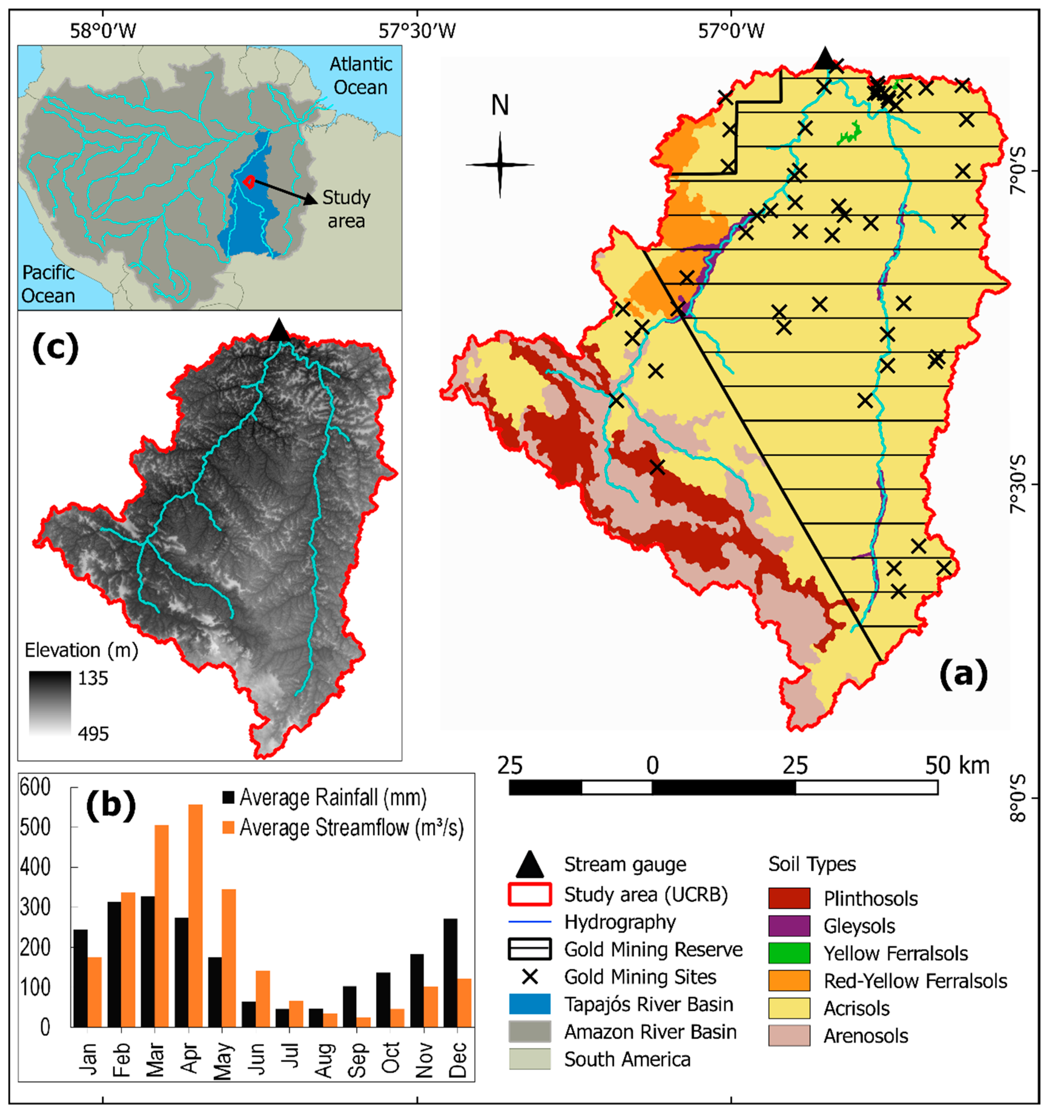
2.1. Study Area

The Upper Crepori River Basin (UCRB) (Figure 1a) is a sub-basin of the Tapajós River Basin, located in the central south of the Brazilian Amazon, and it drains an area of approximately 5924 km². The climate is classified as Ami, by Köppen classification, which stands for tropical humid climate, with a short dry season and average temperatures between 22 °C and 26 °C [32,33]. Precipitation in this region is mainly caused by intense convective processes, resulting in high average annual rates between 2000 and 2250 mm [32,33]. The rainy season occurs between October and May [34], and, overall, the season of river high-flow happens between January and June, whereas the season of low-flow occurs between June and December [35] (Figure 1b). The main soil types in the UCRB are Acrisols, Arenosols, and Plinthosols (Figure 1a). The Brazilian Amazonian soils are known to be highly leached, deep, clayey, and highly porous [36], playing an important role in the hydrology of the Basin. UCRB presents low elevations (from 135 m to up to 495 m) (Figure 1c) and low slopes, which characterizes its relief as low and flat, and vegetation comprises of both dense and open ombrophilous forest (tropical rainforest) [33].

The main economic activity in the Crepori Basin is small-scale gold mining, with several gold mining sites spread all over the basin, and even outside the established Gold Mining Reserve (Figure 1a). On the other hand, logging, agriculture, and pasture are still incipient, resulting in low large-scale deforestation rates [6]. However, sketchy and illegal infrastructures used by miners, such as small roads and airstrips, are important drivers for increasing human settlements [5,6,37] that potentially lead to an increase in future deforestation [1,38], mainly under a less effective environmental legislation. Moreover, the construction of a series of dams in the Tapajós River are planned in the region near the Crepori River Basin [8]. In addition, gold prices and new mining legislation can possibly stimulate the opening of new gold mining sites in the region [6], fueling the expectations of population growth and intense LCC in the near future [38,39].

2.2. Method and Data

The Soil and Water Assessment Tool (SWAT) [40] was applied in this study to model the impacts of LCC on the hydrologic regime of the UCRB. Within the model framework, land cover scenarios of LCC that occurred over the last 40 years were applied to represent past and recent LCC, whereas future LCC scenarios were applied considering two different policy conditions: “Business as Usual”, and “Governance” [31].

Data Used for Model Set Up

Hydrological modelling with SWAT requires spatial data that represent key basin characteristics affecting its hydrology, such as topography, land cover, soil types, and climate (

Table 1. Model Input Data.

Swat Input Data	Spatial Resolution/Scale	Source
Daily Precipitation (1998–2012)	0.25° (~30 km)	TRMM 3B42 Daily v.7 [41]
Daily Temperature (1998–2012)	0.70° (~80 km)	ERA Interim Daily Product [42]
Digital Elevation Model	1 arc second (~30 m)	SRTM [43]
Soil Types Map	1:250,000	IBGE [44]
Land Cover Maps (years: 1973, 1998, 2003 and 2010)	30 m	Classification of Landsat5/TM Images [6,45]
Daily Observed Streamflow 1	-	ANA [35]

¹ One stream gauge, located at the basin’s outlet (Figure 1a), with observed streamflow data corresponding to the period between 2003 and 2012.

). While rainfall is the primary climatic driver, observed streamflow data were also required for model calibration and validation.

● Climate data

Daily precipitation estimates were provided by the TMPA 3B42 v.7 product from the Tropical Rainfall Measuring Mission (TRMM) [41], whereas the daily maximum and minimum air temperatures were derived from the ERA Interim Daily product [42]. The temperature dataset was cross-referenced with in situ measurements from the weather station located near the Basin (at Itaituba city) [32]. It was found that the ERA Interim estimates were overestimating the minimum temperatures from 1998 to 2000 by 1.58 °C, whereas the maximum temperatures were underestimated by 7.58 °C for the entire series. Therefore, a bias correction was applied to the data series, by summing −1.58°C to the minimum temperatures from 1998 to 2000, and 7.58 °C to the maximum temperatures of the entire series. Similarly, the precipitation data from the TRMM were also cross-referenced to the rain gauge measurements at Itaituba station, but no systematic biases were observed. Moreover, rainfall estimates from the 3B42 product were validated for the whole of the Tapajós Basin by Collischonn et al. [46]. The authors state that TRMM estimates are reliable and may be used as rainfall input for hydrological modelling in the Tapajós region where the rain gauge network is sparse, which is the case in the UCRB. Since no station data were available on wind speed, relative humidity, and solar radiation in the region, the Hargreaves method [47] was selected to calculate the basin’s potential evapotranspiration.

● Elevation and topography

The elevation data was derived from the Digital Elevation Model (DEM) (Figure 1c) provided by the Shuttle Radar Topography Mission (SRTM), with 1 arc second (~30 m) of spatial resolution [43]. The watershed boundary, its slopes, and the drainage network were retrieved from the DEM, and used to define the Hydrological Response Units (HRU). HRUs were, in turn, defined as areas with homogeneous land cover, soil type, and slope, for which the model simulated the hydrological variables, such as streamflow, evapotranspiration, and groundwater [40].

● Soil data and parameterization

The soil map made available by the Brazilian Institute of Geography and Statistics (IBGE) [44] (Figure 1a) was combined with the soil texture and depth information retrieved from the databases of the RADAMBRASIL project [48], the Brazilian Agricultural Research Corporation (EMBRAPA) [49,50], and the Brazilian National Agricultural Research Department of the Brazilian Ministry of Agriculture (DNPEA/MA) [51]. Soil hydrological groups and maximum root depths were also derived from the literature [52,53]. Pedotransfer functions, specifically derived for tropical and Amazonian soils, were applied to estimate key soil hydraulic parameters, such as the Saturated Hydraulic Conductivity [54,55,56,57], Soil Bulk Density [58], and Available Water Capacity [54,57,59].

● Definition of Land cover scenarios

The impacts of LCC on the UCRB streamflow were assessed by running the hydrologic simulations using four land cover scenarios that represent three periods (past, recent, and future land cover conditions). The first scenario was the land cover map corresponding to the year 1973 [6] (Figure 2), which represents a quasi-pristine land cover condition, since LCC in the UCRB has become noticeable only at the beginning of the 1980’s as result of the gold rush [60]. This land cover scenario was defined by classifying Landsat5/TM scenes featuring the UCRB at 1973. The small gold mining sites present in the basin at 1973, as well as those present in the other scenarios, were classified as barren land, since the SWAT model database does not have a specific land cover class for gold mining sites. The second scenario represents more recent LCC and is represented by the UCRB’s land cover maps of 1998, 2003, and 2010 (Figure 2), which correspond to the years with the highest LCC for the period from 1998 to 2012 [61]. Landsat5/TM scenes of these years were processed using supervised classification techniques to map the land cover classes as: Forest, pasture, barren land, and open water. These maps were updated during the simulation and, therefore, are hereafter referred as one single scenario: 1998–2003–2010. The third and fourth scenarios represent potential future LCC, projected for 2050, under different policy conditions: The “Business as Usual” (BAU_2050) and the “Governance” (GOV_2050) scenarios (Figure 2). These scenarios were developed by Soares-Filho et al. [31], using the SimAmazonia model and are based on policy-sensitive simulations of future patterns of deforestation at the Amazon Basin, from 2002 to 2050 [31,62]. The BAU_2050 scenario was built by projecting the deforestation rates, estimated from remote sensing monitoring images from 1997 to 2002, and adding the effect of paving major roads in the region. In addition to this, the GOV_2050 scenario also assumed a 50% limit imposed for deforested land within each basin’s sub region, as well as assuming that existing and proposed Protected Areas play a decisive role in limiting deforestation [31,62].

● Observed streamflow

Observed streamflow data was required for model calibration and validation. The only stream gauge located at the UCRB (Figure 1a) recorded observed streamflow at the basin’s outlet, mainly from 2003 to 2012. The data is made available by the Brazilian National Water Agency (ANA) [35] and was divided into two datasets: From 2003 to 2009, for model calibration, and from 2010 to 2012, for model validation.

2.3. Model Set Up

SWAT divides the UCRB into sub-basins based on topographical information, which are, in turn, divided into HRU, based on their land cover and soil type. In this study, the UCRB was divided into 33 sub-basins with a total of 274 HRUs. Equation (1) is the central equation in SWAT that governs the water balance in the basin, as represented by the different hydrological variables [40].

$$S{W}_t=S{W}_0+{\displaystyle \sum }_{i=1}^t\left(R_{day i}-Q_{surf i} -E_{a i}-w_{seep i}-Q_{gw i}\right)$$

(1)

where SW_t is the final soil water content (mm H₂O); SW₀ is the initial soil water content (mm H₂O); t is the time (days); R_{day i} is the precipitation on the day i (mm H₂O); Q_{surf i} is the surface runoff on the day i (mm H₂O); E_{a i} is the evapotranspiration on the day i (mm H₂O); w_{seep i} is the amount of water from the soil profile inflowing to the vadose zone on the day i (mm H₂O); and Q_{gw i} is the base flow on the day i (mm H₂O).

2.4. Sensitivity Analysis, Model Calibration and Validation, and Scenarios Application

The period between 1998 and 2002 was used for the model ‘spin-up’ stage, when the model is run until physically sensible initial conditions are set, especially for the soil moisture. The period between 2003 and 2009 was used for calibration, whereas the period between 2010 and 2012 was used for model validation. Land cover maps of 1998, 2003, and 2010 were updated during the model spin-up, calibration, and validation. Thus, this dynamic land cover map is referred to as a single scenario: 1998–2003–2010.

The automatic calibration of a large number of parameters included in conceptual and semi-distributed models, such as SWAT, can be ineffectively time-consuming and computationally demanding. Therefore, the sensitivity analysis was performed to select the set of parameters that have a larger influence on the model’s results, optimizing the calibration procedure. Also, according to Yang et al. [63], model calibration should consider knowledge of hydrological processes in the basin. Thus, key hydrological processes, such as evapotranspiration and groundwater flow, should be adjusted first, using a manual calibration procedure (trial and error) guided by expert knowledge and initial values derived from the literature [64,65,66,67,68,69]. This procedure was applied until the average rate of annual evapotranspiration and the average rate of annual groundwater flow were comparable to rates reported for similar regions near the Crepori Basin [30,70,71,72,73]. Then, using the SWAT-CUP tool [74], the parameters’ global sensitivity analysis was performed. In this approach, the parameter sensitivity was assessed by performing a t-test on a regression relating the objective function values (regarding the model’s output) against the parameters values, which were sampled using the Latin Hypercube Sampling (LHS) [74]. Next, the most sensitive parameters were ranked, from the most sensitive to the least sensitive, and included in the automatic calibration, which was performed using the Parameter Solution (ParaSol) optimization algorithm [75]. The model was then validated against an observed streamflow dataset that was not used in the calibration procedure. Finally, the model performance was assessed for the entire period of the rainfall data used for the simulations (2003 to 2012), using the Coefficient of determination (R²) (Equation (2)), the Nash-Sutcliffe Efficiency (NSE) [76] (Equation (3)), Percent Bias (PBIAS) [77] (Equation (4)), and the Root Mean Squared Error Observations Standard Deviation Ratio (RSR) [78] (Equation (5)), as recommended by Moriasi et al. [79].

$$R^2=1-\frac{{\left[{{\displaystyle \sum }}_{i=1}^n\left(Q_{obs,i}-{\overline{Q}}_{obs}\right)\left(Q_{sim,i}-{\overline{Q}}_{sim}\right)\right]}^2}{{{\displaystyle \sum }}_{i=1}^n{\left(Q_{obs,i}-{\overline{Q}}_{obs}\right)}^2{{\displaystyle \sum }}_{i=1}^n{\left(Q_{sim,i}-{\overline{Q}}_{sim}\right)}^2}$$

(2)

$$NSE=1-\frac{{{\displaystyle \sum }}_{i=1}^n{\left(Q_{obs,i}-Q_{sim,i}\right)}^2}{{{\displaystyle \sum }}_{i=1}^n{\left(Q_{obs,i}-{\overline{Q}}_{obs}\right)}^2}$$

(3)

$$PBIAS=100\times \frac{{{\displaystyle \sum }}_{i=1}^n\left(Q_{obs,i}-Q_{sim,i}\right)}{{{\displaystyle \sum }}_{i=1}^n{Q}_{obs,i}}$$

(4)

$$RSR=\frac{RMSE}{STDE{V}_{obs}}=\frac{\sqrt{{{\displaystyle \sum }}_{i=1}^n{\left(Q_{obs,i}-Q_{sim,i}\right)}^2}}{\sqrt{{{\displaystyle \sum }}_{i=1}^n{\left(Q_{obs,i}-{\overline{Q}}_{obs}\right)}^2}}$$

(5)

where n is the number of observed data, Q_obs,i is the observed streamflow on the day or month i, ${\overline{Q}}_{obs}$ is the average observed streamflow, Q_sim,i is the streamflow simulated on the day or month i, and ${\overline{Q}}_{sim}$ is the average simulated streamflow.

To evaluate the impacts of LCC on the hydrological regime of the UCRB, the calibrated model was run separately for each land cover scenario (past: 1973; recent: 1998–2003–2010; and future: 2050 ‘BAU_2050’, and ‘GOV_2050’), using the same rainfall dataset (corresponding to the period between 1998 and 2012, with 1998 to 2002 used for model spin-up—i.e., with ten years’ simulation period) for each run.

3. Results

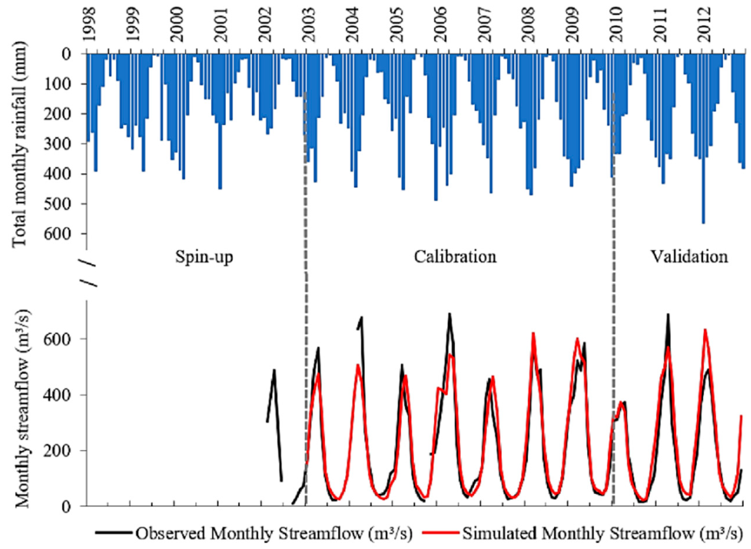
3.1. Sensitivity Analysis, Model Calibration, Validation, and Performance Assessment

As result of the sensitivity analysis, 14 parameters were defined as significantly sensitive (p-value < 0.05) (

Table 2. Most sensitive parameters included in the automatic calibration, and their initial and calibrated values.

Sensitivity Ranking #	Parameter Code	Description	Initial Value	Calibrated Range	Best Calibrated Value
1	GWQMN.gw	Threshold depth water in the shallow aquifer required for return flow to occur (mm H2O)	1000	0.00–439.30	198.48
2	ALPHA_BNK.rte	Baseflow alpha factor for bank storage (days)	0	0.00–1.00	0.051
3	GW_DELAY.gw	Groundwater delay time (days)	31	1.00–69.94	8.21
4	ALPHA_BF.gw	Baseflow alpha factor (1/days)	0.048	0.026–1.00	0.58
5	SOL_AWC(2).sol_PAST 1	Available water capacity of the soil layer (mm H2O/mm soil)	Variable 4	0.97–1.05	1.004 3 (unitless)
6	SOL_AWC(1).sol_PAST 1		Variable 4	0.975–1.05	1.018 3 (unitless)
7	SOL_AWC(3).sol_FRSE 1		Variable 4	0.97–1.05	1.005 3 (unitless)
8	CN2.mgt_LV_FRSE 2	Initial SCS runoff curve number for moisture condition II (-)	30	30.00–36.00	33.08
9	REVAPMN.gw_FRSE 1	Threshold depth of water in the shallow aquifer for “revap” or percolation to the deep aquifer to occur (mm H2O)	614	0.00–1345.25	572.85
10	CN2.mgt_FF_FRSE 2	Initial SCS runoff curve number for moisture condition II (-)	77	77–79	78.25
11	SOL_K(3).sol_FRSE 1	Saturated hydraulic conductivity (mm/h)	Variable 4	0.95–1.10	1.008 3 (unitless)
12	CN2.mgt_LV_PAST 2	Initial SCS runoff curve number for moisture condition II (-)	30	36.71–68.00	56.29
13	SOL_BD(1).sol_PAST 1	Moist bulk density (Mg/m3 or g/cm3)	Variable 4	0.95–1.049	0.982 3 (unitless)
14	CH_K2.rte	Effective hydraulic conductivity in main channel alluvium (mm/h)	0	3.24–130.00	39.37

¹ Numbers (1, 2, 3) refer to the soil layer number, whereas the codes FRSE and PAST refer to the land covers from the SWATv.2012 database ‘Forest Evergreen’ and ‘Pasture’, respectively; ² Codes LV and FF refer to the soil types: Red Yellow Latosol and Plinthosols, respectively; ³ Calibrated values to be multiplied by the initially estimated parameter values (Table A1); ⁴ Initial values of soil parameters vary according to soil type and layer (Table A1).

), including several groundwater parameters. All 14 most sensitive parameters were included in the automatic calibration, which resulted in the calibrated range and the best calibrated values presented in Table 2. Since data and detailed information about the subsurface water in the Crepori region are scarce, parameter values related to groundwater (ALPHA_BF, ALPHA_BNK, GW_DELAY, GWQMN, and REVAPMN_FRSE) (Table 2) were only defined in the calibration procedure, respecting the limits of physically meaningful values indicated by Neitsch et al. [40]. Sensitive soil parameters were calibrated for the first layers and according to the land cover type (Table 2), since land cover substantially affects the soil’s physical-chemical properties, particularly in the first soil layers [30,80,81].

The calibrated values for soil bulk density (SOL_BD), available water capacity (SOL_AWC), and saturated hydraulic conductivity (SOL_K) agrees with values indicated by Tomasella and Hodnett [36] for Amazonian soils (0.7–1.2 Mg/m³ for bulk density, around 0.7 mm·H₂O/mmsoil for available water capacity, and values up to 1000 mm/h for saturated hydraulic conductivity). High saturated hydraulic conductivity values are particularly calibrated for soils covered with forest, which is associated to high root development that enhances the soil permeability [53,82]. The curve number parameter (CN2) is related to the runoff production, and their relatively low values calibrated for Red-Yellow Ferralsols under forested areas (Table 2) confirms the high infiltration expected in forested areas [82,83]. On the other hand, high values of the curve number adjusted for Plinthosols under forested areas (Table 2) were associated to the soil type, since the Plinthosols are characterized by the plinthic horizon, which reduces the infiltration and, consequently, increases the runoff [84]. The adjusted value of the effective hydraulic conductivity in the main channel alluvium (CH_K2) (Table 2) indicates that the Crepori river bed material is mainly characterized by sand and gravel mixture with a low silt-clay content [85], which is corroborated by ICMBio [33] and is also in accordance with the classification of Tapajós Basin streams as clear-water rivers with low concentrations of suspended materials [86]. No parameter related to the deep aquifer was significantly sensitive, indicating that aquifers eventually present in the UCRB have low productivity and low interaction with surface hydrology. This is also corroborated by the fact that the basin is located at the Hydrogeological Province of the Brazilian Shield [87], which typically presents fractured aquifers that are usually deep, sealed, and of low production [88]. The best calibrated parameter values (Table 2) led to a mean evapotranspiration rate of around 54% of the mean annual rainfall, which corresponds to those rates reported in the literature for other Amazon regions like the UCRB [70,71,72,73]. The groundwater parameters were adjusted in such a way that the streamflow simulated for the dry months equaled that observed at the river gauge.

The simulated streamflow matched the observed streamflow and was in synchrony with the variability in the rainfall data (Figure 3), for both calibration and validation periods (Figure 3,

Table 3. Coefficients for assessing the model performance, according to Moriasi et al. [79].

Period	Number of Observed Data	R2	NSE	Classification	RSR	Classification	PBIAS (%)	Classification
Calibration period	87	0.84	0.84	Very good	0.40	Very good	3.56	Very good
Validation period	36	0.84	0.84		0.40		−18.46	Good
Entire series	123	0.86	0.84		0.40		−2.44	Very good

). The model’s performance for the calibration, validation, and the entire period of rainfall used for model simulations (2003–2012) can be classified as ‘good’ and ‘very good’, according to Moriasi et al. [79] (Table 3).

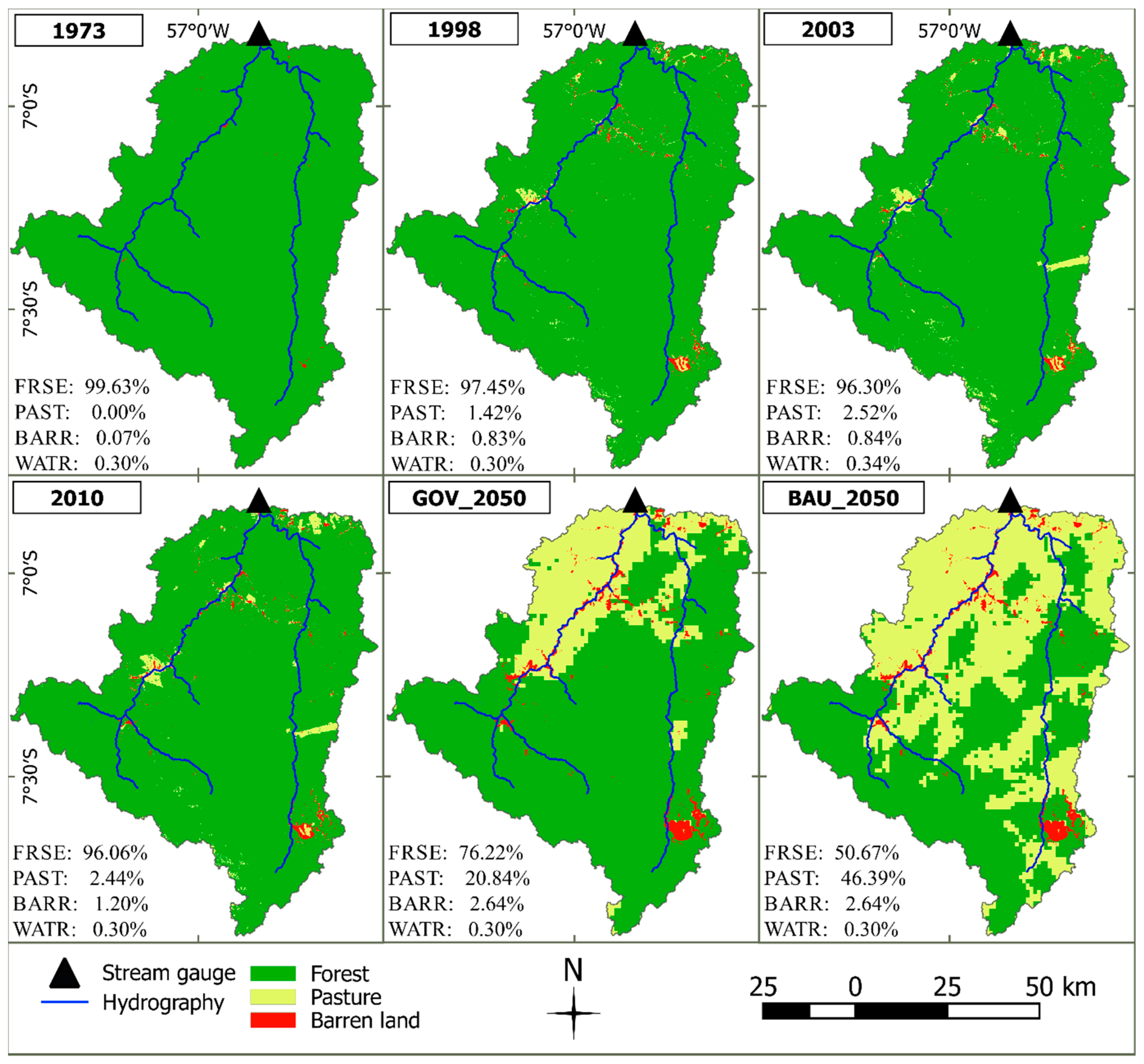
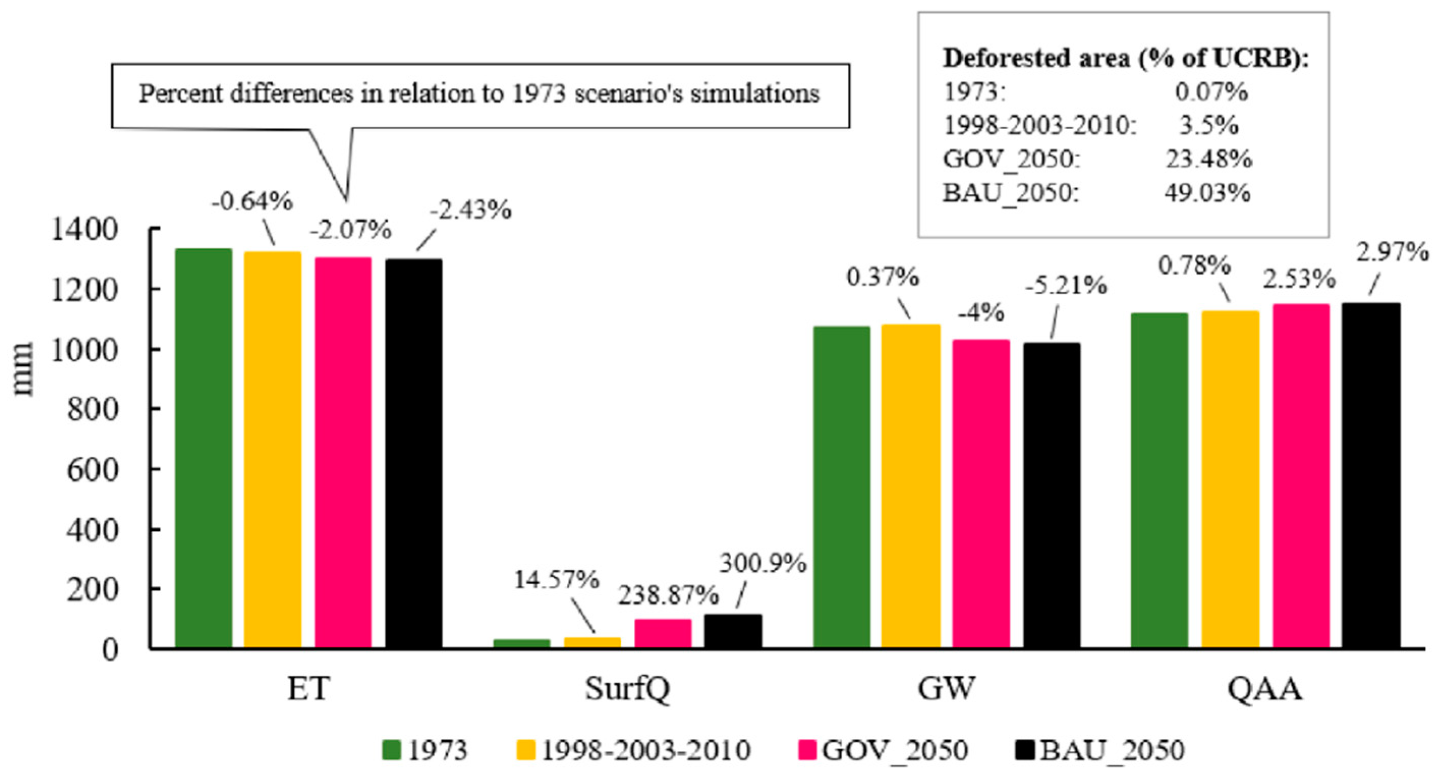
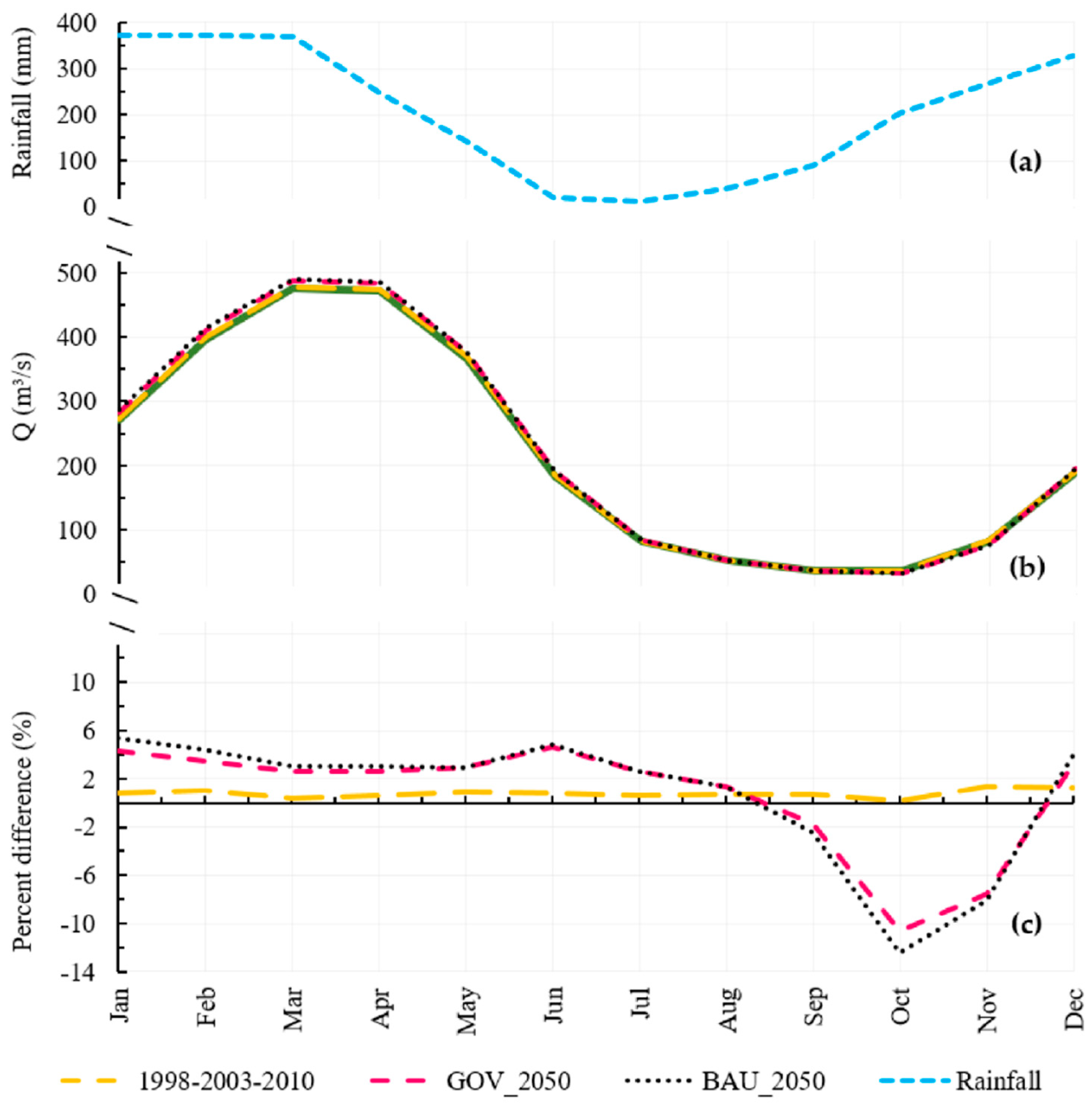
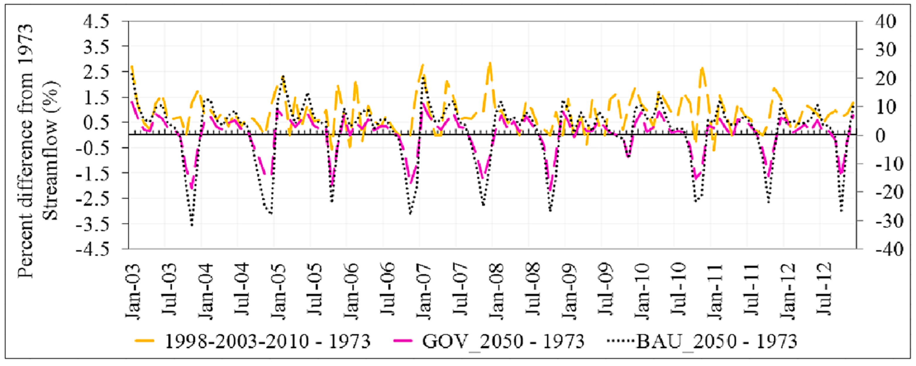
3.2. Streamflow Simulations Corresponding to Land Cover Scenarios

Streamflow simulations were performed for the four land cover scenarios: 1973, 1998–2003–-2010, BAU_2050, and GOV_2050. The mean monthly rainfall for the period from 2003 to 2012 and the corresponding mean monthly streamflow simulated with each of the four land cover maps are displayed in Figure 4. To better visualize the effects of LCC on the streamflow, Figure 4c shows the percent differences between the monthly average streamflow simulated for 1998–-2003–2010, GOV_2050, and BAU_2050 scenarios (${\overline{Q}}_{1998-2003-2010;\mathrm{GOV}\_2050;\mathrm{BAU}\_2050}$), and the corresponding monthly average streamflow simulated for the 1973 scenario (${\overline{Q}}_{1973}$), which is considered as the ‘baseline’.

The $\overline{Q}$ curve simulated for all scenarios displays a slight delay in comparison to the rainfall curve (Figure 4a,b), indicating that the UCRB has a lag-time response to the rainfall events of approximately 1 month. The starting and ending month of both high-flow (January to June) and low-flow (June to December) remained unchanged amongst the $\overline{Q}$ curves simulated for all LCC scenarios (Figure 4b). This indicates that, on average, none of the LCC scenarios used in this study was sufficient to noticeably change the river’s seasonal streamflow dynamics of the UCRB. The percent differences between $\overline{Q}$ values, simulated using the 1998–2003–2010 scenario and that simulated using 1973 scenario (Figure 4c), show that the deforestation that occurred between 1973 and 2012 was not sufficient to noticeably increase the $\overline{Q}$ at an annual scale, and resulted in an increase in streamflow of about only 1% throughout the seasons. On the other hand, the change in $\overline{Q}$, resulting from simulations with the GOV_2050 and BAU_2050 scenarios, shows higher values during the high-flow season and at the beginning of the low-flow season, with maximum increase rates of 4% and 5%, respectively (Figure 4c). During most of the low-flow season (from mid-August to mid-November), $\overline{Q}$, simulated using the GOV_2050 and BAU_2050 scenarios, showed a reduction of up to 10% and 12%, respectively, for the month of October, whereas the $\overline{Q}$, simulated using the 1998–2003–2010 scenario, showed the smallest increase rate (0.2%) for the same month (Figure 4c). The reduction of streamflow during the low-flow season is even larger when analyzing the percent differences between the monthly streamflow simulated for each month of the time series (from 2003 to 2012) (Figure 5).

Since the monthly mean streamflow was not averaged over the entire simulation period, the percent differences showed in Figure 5 display higher absolute values than those presented in Figure 4c. The 1998–2003–2010 scenario still shows relatively small streamflow increase and reduction rates (up to 2.5% and less than 0.5%, respectively), compared to the baseline (simulation using 1973 land cover scenario). Nevertheless, the overall percent differences between the streamflow simulated for the 1998–2003–2010 scenario and the 1973 scenario are positive, indicating that the small LCC between both scenarios was sufficient to depict a trend of an increase in streamflow, at a monthly time-scale analysis (Figure 5). The streamflow simulated using the GOV_2050 and BAU_2050 scenarios showed increases as high as 11% and 22%, respectively, throughout the series (during the high-flow season), and reduction rates as high as 19% and 32%, respectively, during the low-flow season (Figure 5). Regarding the other water balance components (WBC) as an annual average, the increased UCRB deforestation depicts a trend of increasing Surface Runoff (SurfQ) and Average Annual Streamflow (Q_AA), with decreasing Groundwater (GW) and Evapotranspiration (ET) (Figure 6). The percent differences of the WBC between the 1973 and 1998–2003–2010 scenarios are small (Figure 6), since the deforested areas in these scenarios are relatively similar (Figure 2) and, therefore, did not affect the basin’s hydrology in a noticeable way. On the other hand, the WBC simulated for the GOV_2050 and BAU_2050 scenarios varies noticeably amongst all of them, especially for the SurfQ and GW (Figure 6), resulting in higher percent differences (Figure 6).

4. Discussion

A hydrological modelling approach was implemented to study the possible impacts of contemporary and future LCC on the hydrology of the UCRB. The possibility of updating the land cover of the SWAT model during the model run helped in capturing the LCC dynamic and achieving good overall performance results. The manual adjustment of parameters, prior to the automatic calibration, based on previous knowledge of the physiographic characteristics of the basin, helped in defining the optimal parameter set and improve the reliability of the simulations. Although small, the deforestation that occurred in the basin between 1973 and 2012 was sufficient to depict a trend of increases in the streamflow at a monthly time-scale analysis (Figure 5), corresponding to the increase in deforested areas, which is in accordance with the findings from previous studies in Amazon basins and other tropical regions [29,30,89,90]. This trend was more clearly displayed when simulating discharge during the high-flow season corresponding to the future BAU_2050 and GOV_2050 scenarios (Figure 4c). At the same time, the future scenarios also show a dramatic percent decrease in Q during the low-flow season, with simulations corresponding to the BAU_2050 scenario resulting in the highest percent change in Q, in relation to simulations corresponding to the 1973 quasi-pristine scenario (Figure 4c and Figure 5). This shows that the potential deforestation by 2050, based on both the BAU_2050 and GOV_2050 scenarios, can remarkably change Q and other components of the water balance, especially by increasing SurfQ and Q, and decreasing GW and ET (Figure 6). SurfQ was the only WBC that showed a substantial increase in the annual average values, following the increase of deforestation (Figure 6), indicating that the SurfQ was the main component responsible for the slight increase in Q_AA throughout the scenarios. Forest removal in tropical Basins typically reduces interception and ET, and increases SurfQ and Q during the rainy season [29,90,91]. However, during the dry season, Q is reduced when deforested areas increase (Figure 4c). Even though, during the dry season, deforestation has similar effects on interception, ET, and SurfQ, the rainfall rates are lower in this season and, therefore, the increase of SurfQ does not seem to noticeably contribute to Q. Besides, the GW is reduced as result of deforestation, since most of the water that enters the basin during the rainy season (as rainfall) is lost as SurfQ and Q, and does not contribute to GW storage. Furthermore, it is reported that the amount of water that infiltrates into the soil decreases from 130 mm to 60 mm throughout the dry season, rarely reaching more than 1m of Amazonian soil depth [92], which contributes to the critical reduction of GW in that season. Finally, since Q during the dry season is more dependent on the GW, the reduction of the GW results in the reduction of Q during the dry season.

The findings of this study support the “Sponge Effect Hypothesis” [80,91], which identifies tropical forests as being responsible for reducing peak discharge during rainy seasons (due to low SurfQ and high ET), while acting as a ‘sponge’ during the dry season, allowing higher soil infiltration, increasing GW, and, therefore, resulting in higher Q than those from deforested areas [80,91]. However, while it is generally understood that deforestation in tropical regions usually leads to an increase in high flows, the impacts of deforestation on low flows is known to be more difficult to predict [93].

The estimated past and potential future impacts of LCC on the Q and water balance indicate that deforestation increases in the UCRB may result in higher streamflow and lower low-flows during high-flow and low-flow seasons, respectively, even when considering successful implementation of environmental regulations and policies, as in the GOV_2050 scenario. In addition, changes in the water balance may also impact the water quality of the Crepori River, especially during the low-flow season, which is when small-scale gold mining activity intensifies, resulting in high sediment loads to the river [5]. The reduction of Q, simulated for the low-flow season in the GOV_2050 and BAU_2050 scenarios, may increase sediment concentration, since there will be less discharge in the river to dilute and wash the sediments and other pollutants. For the various dam projects that are under consideration in the Tapajós River, downstream of the Crepori River [8], these impacts on the streamflow and, potentially, on the water quality can increase maintenance costs of hydropower plants and periods with lower water volume storage, potentially resulting in lower power generation rates [27,94]. On the other hand, the predicted increase in streamflow during the high-flow season represents an increase in flood risks in cities and indigenous lands along the river. It is also worth stating that the forest removal may reduce rainfall rates, potentially reducing Q and also affecting the climate in distant areas [19,20,21,22]. This climate feedback can be even more critical, since the reduction of rainfall rates hampers forest regeneration.

Since the focus of this study was to analyze the impacts of LCC alone on the streamflow, climate implications of deforestation were not taken into account. However, more accurate predictions of LCC impacts on the hydrology of the UCRB must consider the climate feedback, as well as finer time scale analysis, such as a daily scale. These should be the focus of other future studies.

5. Conclusions

This study investigated the impacts of historical and potential future deforestation on the hydrology of the Upper Crepori River Basin (UCRB) using a hydrological modelling approach. The main findings of the study are:

Deforestation that occurred in the UCRB since human exploration in the early 1970 s until recent years (1998–2012) was small, and was not sufficient to change the streamflow more than 2.5%, in an annual basis, and not sufficient to noticeably alter the annual water balance of the basin.

Hydrologic model simulation, with land cover scenarios developed by Soares-Filho et al. [30] for 2050, in both conditions of ‘Business as Usual’ and ‘Governance’ led to an increase in streamflow during the high-flow season and a decrease in streamflow in the low-flow season, intensifying river high-flows and low-flows events.

The projected deforestation for 2050 is also found to alter the water balance of the basin, increasing surface runoff and streamflow, and reducing groundwater and evapotranspiration.

Since both future land cover scenarios, GOV_2050 and BAU_2050, led to very similar results of the hydrological variables, this study shows that, even if conservation policies are respected, the expected future deforestation can still compromise the water resources in the UCRB, directly affecting local human communities, the biota, and possible planned hydropower generation.

In general, this study presents important analysis and information for water resources management and land use planning in a portion of the Tapajós Basin, regarding future water availability with respect to land cover change. Further studies are still needed to better understand the impacts of deforestation on the hydrology, including possible climate feedbacks and finer time-scale analysis.

References

1. Fearnside, P.M. Deforestation in Brazilian Amazonia: The effect of population and land tenure. Ambio 1993, 22, 537–545. [Google Scholar]
2. Nepstad, D.; Soares-Filho, B.S.; Merry, F.; Lima, A.; Moutinho, P.; Carter, J.; Bowman, M.; Cattaneo, A.; Rodrigues, H.; Schwartzman, S.; et al. The end of deforestation in the Brazilian Amazon. Science 2009, 326, 1350–1351. [Google Scholar] [CrossRef] [PubMed]
3. Vasconcelos, P.G.A.; Angelo, H.; Almeida, A.N.; Matricardi, E.A.T.; Miguel, E.P.; De Souza, A.N.; De Paula, M.F.; Goncalez, J.C.; Joaquim, M.S. Determinants of the Brazilian Amazon deforestation. Afr. J. Agric. Res. 2017, 12, 169–176. [Google Scholar] [CrossRef]
4. Kalamandeen, M.; Gloor, E.; Mitchard, E.; Quincey, D.; Ziv, G.; Spracklen, D.; Spracklen, B.; Adami, M.; Aragão, L.E.O.C.; Galbraith, D. Pervasive rise of small-scale deforestation in Amazonia. Sci. Rep. 2018, 8, 1600. [Google Scholar] [CrossRef] [PubMed]
5. Lobo, F.L.; Costa, M.P.; Novo, E.M. Time-series analysis of Landsat-MSS/TM/OLI images over Amazonian waters impacted by gold mining activities. Remote Sens. Environ. 2015, 157, 170–184. [Google Scholar] [CrossRef]
6. Lobo, F.L.; Costa, M.; Novo, E.M.L.M.; Telmer, K. Distribution of artisanal and small-scale gold mining in the Tapajós River Basin (Brazilian Amazon) over the Past 40 Years and Relationships with Water Siltation. Remote Sens. 2016, 8, 579. [Google Scholar] [CrossRef]
7. Ferreira, J.; Aragão, L.E.O.C.; Barlow, J.; Barreto, P.; Berenguer, E.; Bustamante, M.; Gardner, T.A.; Lees, A.C.; Lima, A.; Louzada, J.; et al. Brazil’s environmental leadership at risk. Science 2014, 346, 706–707. [Google Scholar] [CrossRef] [PubMed]
8. Latrubesse, E.M.; Arima, E.Y.; Dunne, T.; Edward, P.; Baker, V.R.; D’Horta, F.M.; Wight, C.; Wittmann, F.; Zuanon, J.; Baker, P.A.; et al. Damming the rivers of the Amazon basin. Nature 2017, 546, 363–369. [Google Scholar] [CrossRef] [PubMed] [Green Version]
9. Biggs, T.; Dunne, T.; Martinelli, L. Natural Controls and Human Impacts on Stream Nutrient Concentrations in a Deforested Region of the Brazilian Amazon Basin. Biogeochemistry 2004, 68, 227–257. [Google Scholar] [CrossRef]
10. Oestreicher, J.S.; Lucotte, M.; Moingt, M.; Bélanger, É.; Rozon, C.; Davidson, R.; Mertens, F.; Romaña, C.A. Environmental and anthropogenic factors influencing mercury dynamics during the past century in floodplain lakes of the Tapajós River, Brazilian Amazon. Arch. Environ. Contam. Toxicol. 2017, 72, 11–30. [Google Scholar] [CrossRef] [PubMed]
11. Mol, J.H.; Ouboter, P.E. Downstream effects of erosion from small-scale gold mining on the instream habitat and fish community of a small neotropical rainforest stream. Conserv. Biol. 2004, 18, 201–214. [Google Scholar] [CrossRef]
12. Barlow, J.; Lennox, G.D.; Ferreira, J.; Berenguer, E.; Lees, A.C.; Mac Nally, R.; Thomson, J.R.; Ferraz, S.F.; Louzada, J.; Oliveira, V.H.; et al. Anthropogenic disturbance in tropical forests can double biodiversity loss from deforestation. Nature 2016, 535, 144–147. [Google Scholar] [CrossRef] [PubMed]
13. Skole, D.; Tucker, C. Tropical deforestation and habitat fragmentation in the Amazon: Satellite data from 1978 to 1988. Science 1993, 260, 1905–1910. [Google Scholar] [CrossRef] [PubMed]
14. Renó, V.; Novo, E.; Escada, M. Forest fragmentation in the lower Amazon floodplain: Implications for biodiversity and ecosystem service provision to riverine populations. Remote Sens. 2016, 8, 886. [Google Scholar] [CrossRef]
15. Dos Santos, V.; Laurent, F.; Abe, C.; Messner, F. Hydrologic Response to Land Use Change in a Large Basin in Eastern Amazon. Water 2018, 10, 429. [Google Scholar] [CrossRef]
16. Costa, M.H.; Botta, A.; Cardille, J.A. Effects of large-scale changes in land cover on the discharge of the Tocantins River, Southeastern Amazonia. J. Hydrol. 2003, 283, 206–217. [Google Scholar] [CrossRef]
17. Siqueira Júnior, J.L.; Tomasella, J.; Rodriguez, D.A. Impacts of future climatic and land cover changes on the hydrological regime of the Madeira River basin. Clim. Chang. 2015, 129, 117–129. [Google Scholar] [CrossRef]
18. Bradshaw, C.; Sodhi, N.; Peh, K.; Brook, B. Global evidence that deforestation amplifies flood risk and severity in the developing world. Glob. Chang. Biol. 2007, 13, 2379–2395. [Google Scholar] [CrossRef]
19. Shukla, J.; Nobre, C.; Sellers, P. Amazon Deforestation and Climate Change. Science 1990, 247, 1322–1325. [Google Scholar] [CrossRef] [PubMed] [Green Version]
20. Nobre, A.D. O futuro Climático da Amazônia. Scientific Evaluation Report. 2014. Available online: https://www.socioambiental.org/sites/blog.socioambiental.org/files/futuro-climatico-da-amazonia.pdf (accessed on 8 August 2017).
21. Nazareno, A.G.; Laurence, W.F. Brazil’s drought: Beware deforestation. Science 2015, 347, 1427. [Google Scholar] [CrossRef] [PubMed]
22. Alves, L.; Marengo, J.; Fu, R.; Bombardi, R.J. Sensitivity of Amazon Regional Climate to Deforestation. Am. J. Clim. Chang. 2017, 6, 75–98. [Google Scholar] [CrossRef]
23. Refsgaard, J.C.; Abbott, M.B. The role of distributed hydrological modelling in water resources management. In Distributed Hydrological Modelling; Cap.3.Dordrecht; Abbott, M.B., Refsgaard, J.C., Eds.; Kluwer Academic Publishers: Dordrecht, The Netherlands, 1996; ISBN 0-7923-4042-6. [Google Scholar]
24. Loucks, D.P.; Beek, E. Water Resource Systems Planning and Management: An Introduction to Methods, Models and Applications; UNESCO-IHE; Springer: Deltares, The Netherlands, 2017. [Google Scholar] [CrossRef]
25. Liu, J.; Liu, T.; Bao, A.; De Maeyer, P.; Feng, X.; Miller, S.N.; Chen, X. Assessment of Different Modelling Studies on the Spatial Hydrological Processes in an Arid Alpine Catchment. Water Resour. Manag. 2016, 30, 1757–1770. [Google Scholar] [CrossRef] [Green Version]
26. Malagó, A.; Bouraoui, F.; Vigiak, O.; Grizzetti, B.; Pastori, M. Modelling water and nutrient fluxes in the Danube River Basin with SWAT. Sci. Total Environ. 2017, 603, 196–218. [Google Scholar] [CrossRef] [PubMed]
27. Mohor, G.S.; Rodriguez, D.A.; Tomasella, J.; Siqueira, J.L., Jr. Exploratory analysis for the assessment of climate change impacts on the energy production in an Amazon run-of-river hydropower plant. J. Hydrol. Reg. Stud. 2015, 4, 41–59. [Google Scholar] [CrossRef]
28. De Figueiredo, N.M.; Blanco, C.J.C. Water level forecasting and navigability conditions of the Tapajós River-Amazon–Brazil. Houille Blanche 2016, 3, 53–64. [Google Scholar] [CrossRef]
29. Guimberteau, M.; Ciais, P.; Ducharne, A.; Boisier, J.P.; Aguiar, A.P.D.; Biemans, H.; Deurwaerder, H.D.; Galbraith, D.; Kruijt, B.; Langerwisch, F.; et al. Impacts of Future Deforestation and Climate Change on the Hydrology of the Amazon Basin: A Multi-Model Analysis with a New Set of Land-Cover Change Scenarios. Hydrol. Earth Syst. Sci. 2017, 21, 1455–1475. [Google Scholar] [CrossRef]
30. Lamparter, G.; Nobrega, R.L.B.; Kovacs, K.; Amorim, R.S.; Gerold, G. Modelling hydrological impacts of agricultural expansion in two macro-catchments in Southern Amazonia, Brazil. Reg. Environ. Chang. 2018, 18, 19–103. [Google Scholar] [CrossRef]
31. Soares-Filho, B.S.; Nepstad, D.C.; Curran, L.M.; Cerqueira, G.C.; Garcia, R.A.; Ramos, C.A.; Voll, E.; McDonald, A.; Lefebvre, P.; Schlesinger, P. Modelling conservation in the Amazon Basin. Nature 2006, 440, 520. [Google Scholar] [CrossRef] [PubMed]
32. IBAMA, Brazilian Institute of the Environment and Renewable Natural Resources. Floresta Nacional do Tapajós–Management Plan. IBAMA, Belterra; 2004. Available online: http://www.icmbio.gov.br/portal/images/stories/imgs-unidades-coservacao/flona_tapajoss.pdf (accessed on 6 May 2016).
33. ICMBIO, Chico Mendes Institute for Biodiversity Conservation. Plano de Manejo da Floresta Nacional do Crepori, Localizada no Estado do Pará. Management Plan. Curitiba/PR; 2010. Available online: http://www.icmbio.gov.br/portal/images/stories/imgs-unidades-coservacao/crepori_plano%20de%20manejo.pdf (accessed on 2 May 2016).
34. INMET, Brazilian National Institute of Metheorology. Banco de Dados Meteorológicos para Ensino e Pesquisa. Available online: http://www.inmet.gov.br/portal/index.php?r=bdmep/bdmep (accessed on 5 February 2017).
35. ANA, Agência Nacional de Águas. Daily Streamflow Database. Available online: http://www.snirh.gov.br/hidroweb/ (accessed on 4 April 2016).
36. Tomasella, J.; Hodnett, M.G. Pedotransfer functions for tropical soils. Dev. Soil. Sci. 2004, 30, 415–429. [Google Scholar] [CrossRef]
37. Telmer, K.; Costa, M.; Angélica, R.S.; Araújo, E.S.; Maurice, Y. The source and fate of sediment and mercury in the Tapajós River, Pará, Brazilian Amazon: Ground and space-based evidence. J. Environ. Manag. 2006, 81, 101–113. [Google Scholar] [CrossRef] [PubMed]
38. Fearnside, P.M. Deforestation in Brazilian Amazonia. In Oxford Bibliographies in Environmental Science; Wohl, E., Ed.; Oxford University Press: New York, NY, USA, 2017; ISBN 978-0-19936-344-5. [Google Scholar] [CrossRef]
39. Winemiller, K.O.; McIntyre, P.B.; Castello, L.; Fluet-Chouinard, E.; Giarrizzo, T.; Nam, S.; Baird, I.G.; Darwall, W.; Lujan, N.K.; Harrison, I.; et al. Balancing hydropower and biodiversity in the Amazon, Congo and Mekong. Science 2016, 351, 128. [Google Scholar] [CrossRef] [PubMed] [Green Version]
40. Neitsch, S.L.; Arnold, J.G.; Kiniry, J.R.; Williams, J.R. Soil & Water Assessment Tool-Theoretical Documentation Version 2009. Texas Water Resour. Inst. 2011, 647, TR-406. Available online: https://swat.tamu.edu/media/99192/swat2009-theory.pdf (accessed on 10 December 2015).
41. NASA. National Aeronautics and Space Agency. TRMM 3B42 Daily v.7 Product. Available online: https://disc.sci.gsfc.nasa.gov/SSW/#keywords= (accessed on 7 February 2016).
42. ECMWF. European Centre for Medium-Range Weather Forecasts. Era Interim Daily Database. Available online: http://apps.ecmwf.int/datasets/data/interim-full-daily/levtype=sfc/ (accessed on 2 February 2017).
43. USGS. United States Geological Survey. SRTM-Shuttle Radar Topography Mission. Available online: https://earthexplorer.usgs.gov/ (accessed on 5 February 2016).
44. IBGE, Brazilian Institute of Geography and Statistics. Mapa Pedológico da Amazonia Legal 1:250.000. 2016. Available online: Ftp://geoftp.ibge.gov.br/informacoes_ambientais/pedologia/vetores/escala_250_mil/amazonia_legal/ (accessed on 7 February 2016).
45. USGS. United States Geological Survey. Landsat5/TM Archive. Available online: https://earthexplorer.usgs.gov/ (accessed on 3 January 2017).
46. Collischonn, B.; Collishonn, W.; Tucci, C.E.M. Daily hydrological modeling in the Amazon basin using TRMM rainfall estimates. J. Hydrol. 2008, 360, 207–2016. [Google Scholar] [CrossRef]
47. Hargreaves, G.; Hargreaves, G.; Riley, J. Agricultural benefits for Senegal River Basin. J. Irrig. Drain. Eng. 1985, 111, 113–124. [Google Scholar] [CrossRef]
48. Brazil. National Department of Mineral Production. Projeto RADAM. Folha SB.21 Tapajós; Geologia, Geomorfologia, Solos, Vegetação e uso Potencial da Terra. Rio de Janeiro. Available online: https://biblioteca.ibge.gov.br/visualizacao/livros/liv24024.pdf (accessed on 15 November 2016).
49. EMBRAPA/SNLCS. Levantamento de Reconhecimento de Solos e Aptidão Agrícola das Terras do Polo Carajás Estado do Pará. Research Bulletin No. 29. Rio de Janeiro, Brasil; 1984. Available online: https://biblioteca.ibge.gov.br/index.php/biblioteca-catalogo?view=detalhes&id=219908 (accessed on 20 November 2016).
50. EMBRAPA/FAO. Caracterização Físico Hídrica dos Principais Solos da Amazônia Legal: Volume I–Estado do Pará. Technical Report. Belém/PA, Brasil. 1991. Available online: https://ainfo.cnptia.embrapa.br/digital/bitstream/item/48881/1/Boletim-Pesquisa-205-CPATU.pdf (accessed on 17 November 2016).
51. Brazil. Ministry of Agriculture, Divison of Pedological Research. Levantamento de Reconhecimento de Solos de Uma Área Prioritária da Rodovia Transamazônica entre Altamira e Itaituba. Technical Bulletin No. 34. Rio de Janeiro. Brasil. 1973. Available online: https://ainfo.cnptia.embrapa.br/digital/bitstream/item/62724/1/CNPS-BOL.-TEC.-34-73.pdf (accessed on 18 November 2016).
52. Sartori, A.; Lombardi Neto, F.; Genovez, A.M. Classificação Hidrológica de Solos Brasileiros para a Estimativa da Chuva Excedente com o Método do Serviço de Conservação do Solo dos Estados Unidos. Parte I: Classificação. Rev. Bras. Recur. Hídr. 2005, 10, 5–18. [Google Scholar] [CrossRef]
53. Quesada, C.A.; Lloyd, J.; Anderson, L.O.; Fyllas, N.M.; Schwarz, M.; Czimczik, C.I. Soils of Amazonia with particular reference to the RAINFOR sites. Biogeosciences 2011, 8, 1415–1440. [Google Scholar] [CrossRef]
54. Van Genuchten, M.T. A closed form equation for predicting the hydraulic conductivity of unsaturated soils. Soil Sci. Soc. Am. J. 1980, 44, 892–898. [Google Scholar] [CrossRef]
55. Ahuja, L.R.; Naney, J.W.; Green, R.E.; Nielsen, D.R. Macroporosity to Characterize Spatial Variability of Hydraulic Conductivity and Effects of Land Management1. Soil Sci. Soc. Am. J. 1984, 48, 699–702. [Google Scholar] [CrossRef]
56. Tomasella, J.; Hodnett, M.G. Estimating unsaturated hydraulic conductivity of Brazilian soils using soil-water retention data. Soil Sci. 1997, 162, 703–712. [Google Scholar] [CrossRef]
57. Tomasella, J.; Hodnett, M.G.; Rossato, L. Pedotransfer Functions for the Estimation of Soil Water Retention in Brazilian Soils. Soil Sci. Soc. Am. J. 2000, 64, 327–338. [Google Scholar] [CrossRef]
58. Tomasella, J.; Hodnett, M.G. Estimating soil water retention characteristics from limited data in Brazilian Amazonia. Soil Sci. 1998, 16, 190–202. [Google Scholar] [CrossRef]
59. Arnold, J.G.; Kiniry, J.R.; Srinivasan, R.; Williams, J.R.; Haney, E.B.; Neitsch, S.L. Soil and Water Assessment Tool: Input/Output Documentation. Version 2012. 2012. Available online: https://swat.tamu.edu/media/69296/SWAT-IO-Documentation-2012.pdf (accessed on 15 December 2015).
60. Bezerra, O.; Veríssimo, A.; Uhl, C. Impactos da garimpagem de ouro na Amazônia Oriental. Série Amazônia No. 02. Belém/PA: Imazon. 1998. Available online: http://www.ciflorestas.com.br/arquivos/doc_impactos_ocidental_6860.pdf (accessed on 16 May 2017).
61. INPE, Brazilian National Institute for Space Research. PRODES Project. Available online: http://www.obt.inpe.br/prodes/index.php (accessed on 20 December 2016).
62. Soares-Filho, B.S.; Nepstad, D.C.; Curran, L.M.; Voll, E.; Garcia, R.A.; Ramos, C.A.; McDonald, A.J.; Lefebvre, P.A.; Schlesinger, P. LBA-ECO LC-14 Modelled Deforestation Scenarios, Amazon Basin: 2002–2050. Data set. ORNL DAAC 2013. [Google Scholar] [CrossRef]
63. Yang, J.; Liu, Y.; Yang, W.; Chen, Y. Multi-objective sensitivity analysis of a fully distributed hydrologic model WetSpa. Water Resour. Manag. 2012, 26, 109–128. [Google Scholar] [CrossRef]
64. Correa, J.C. Características físico hídricas dos solos latosolo amarelo, podzolico vermelho amarelo e podzol hidromórfico do estado do Amazonas. Pesqui. Agropecu. Bras. 1984, 19, 1317–1322. [Google Scholar]
65. Tomasella, J.; Hodnett, M.G. Soil hydraulic properties and van Genuchten parameters for a oxisol under pasture in central Amazonia. In Amazonian Deforestation and Climate; Victoria, R.L., Gash, J.H.C., Nobre, C.A., Roberts, J.M., Eds.; Wiley: Chichester, UK, 1996; pp. 101–124. ISBN 0-471-96734-3. [Google Scholar]
66. Fajardo, J.D.V.; Ferreira, S.J.F.; Miranda, S.A.F.; Marques Filho, A.O. Características hidrológicas do solo saturado na Reserva Florestal Adolpho Ducke-Amazônia central. Rev. Árvore 2010, 34, 677–684. [Google Scholar] [CrossRef]
67. Williams, M.; Shimabukuro, Y.E.; Rastetter, E.B. LBA-ECO CD-09 Soil and Vegetation Characteristics, Tapajós National Forest, Brazil; Dataset; Oak Ridge National Laboratory Distributed Active Archive Centre: Oak Ridge, TN, USA, 2012. Available online: http://daac.ornl.gov (accessed on 6 February 2017).
68. Costa, M.H.; Cohen, W. LBA-ECO CD-15 LAI and Productivity Data, km 67, Tapajós National Forest: 2003–2004; Dataset; Oak Ridge National Laboratory Distributed Active Archive Centre: Oak Ridge, TN, USA, 2013. Available online: http://daac.ornl.gov (accessed on 18 February 2017).
69. Strauch, M.; Volk, M. SWAT plant growth modification for improved modelling of perennial vegetation in the tropics. Ecol. Model. 2013, 269, 98–112. [Google Scholar] [CrossRef]
70. Shuttleworth, W.J. Evaporation from Amazonian Rainforest. Proc. R. Soc. Lond. B 1988, 233, 321–346. [Google Scholar] [CrossRef]
71. Malhi, Y.; Pegoraro, E.; Nobre, A.D.; Pereira, M.G.P.; Grace, J.; Culf, A.D.; Clement, R. Energy and water dynamics of a central Amazonian rain forest. J. Geophys. Res. 2002, 107, 8061. [Google Scholar] [CrossRef]
72. Tomasella, J.; Hodnett, M.G.; Cuartas, L.A.; Nobre, A.D.; Waterloo, M.J.; Oliveira, S.M. The water balance of Amazonian micro-catchment: The effect of interannual variability of rainfall on hydrological behavior. Hydrol. Process. 2008, 22, 2133–2147. [Google Scholar] [CrossRef]
73. Cuartas, L.A.; Tomasella, J.; Nobre, A.D.; Nobre, C.A.; Hodnett, M.G.; Waterloo, M.J.; De Oliveira, S.M.; Von Randow, R.C.; Trancoso, R.; Ferreira, M. Distributed hydrological modeling of a micro-scale rainforest watershed in Amazonia: Model evaluation and advances in calibrating using the new HAND terrain model. J. Hydrol. 2012, 462–463, 15–27. [Google Scholar] [CrossRef]
74. Abbaspour, K. SWAT-CUP: SWAT Calibration and Uncertainty Programs—A User Manual; Eawag: Duebendorf, Switzerland, 2015; p. 103. [Google Scholar]
75. Van Griensven, A.; Meixner, T. Methods to quantify and identify the sources of uncertainty for river basin water quality models. Water Sci. Technol. 2006, 53, 51–59. [Google Scholar] [CrossRef] [PubMed]
76. Nash, J.E.; Sutcliffe, J.V. River flow forecasting through conceptual models: Part 1. A discussion of principles. J. Hydrol. 1970, 10, 282–290. [Google Scholar] [CrossRef]
77. Gupta, H.V.; Sorooshian, S.; Yapo, P.O. Status of automatic calibration for hydrologic models: Comparison with multilevel expert calibration. J. Hydrol. Eng. 1999, 42, 135–143. [Google Scholar] [CrossRef]
78. Singh, J.; Knapp, H.V.; Arnold, J.G.; Demissie, M. Hydrological modelling of the Iroquois River watershed using HSPF AND SWAT. J. Am. Water Resour. Assoc. 2005, 41, 343–360. [Google Scholar] [CrossRef]
79. Moriasi, D.N.; Arnold, J.G.; van Liew, M.W.; Binger, R.L.; Harmel, R.D.; Veith, T.L. Model evaluation guidelines for systematic quantification of accuracy in watershed simulations. Trans. ASABE 2007, 50, 885–900. [Google Scholar] [CrossRef]
80. Bruijnzeel, L.A. Hydrological functions of tropical forests: Not seeing the soil for the trees? Agric. Ecosyst. Environ. 2004, 104, 185–228. [Google Scholar] [CrossRef]
81. Christoffersen, B.O.; Restrepo-Coupe, N.; Arain, M.A.; Baker, I.T.; Cestaro, B.P.; Ciais, P.; Fisher, J.B.; Galbraith, D.; Guan, X.; Gulden, L.; et al. Mechanisms of water supply and vegetation demand govern the seasonality and magnitude of evapotranspiration in Amazonia and Cerrado. Agric. Forest Meteorol. 2014, 191, 33–50. [Google Scholar] [CrossRef] [Green Version]
82. Ellison, D.; Morris, C.E.; Locatelli, B.; Sheil, D.; Cohen, J.; Murdiyarso, D.; Gutierrez, V.; Van Noordwijk, M.; Creed, I.F.; Pokorny, J.; et al. Trees, forest and water: Cool insights for a hot world. Glob. Environ. Chang. 2017, 43, 51–61. [Google Scholar] [CrossRef]
83. Simmons, L.A.; Anderson, S.H. Effects of logging activities on selected soil physical and hydraulic properties for a claypan landscape. Geoderma 2016, 269, 145–152. [Google Scholar] [CrossRef]
84. Brazilian Agricultural Research Corporation (EMBRAPA). Sistema Brasileiro de Classificação dos Solos; Centro Nacional de Pesquisa de Solos: Rio de Janeiro, Brazil, 2006. p. 306. Available online: https://www.agrolink.com.br/downloads/sistema-brasileiro-de-classificacao-dos-solos2006.pdf (accessed on 19 December 2017).
85. Lane, L.J. Chapter 19: Transmission Losses, SCS-National Engineering Handbook, Section 4, Hydrology; Section 4; US Government Printing Office: Washington, DC, USA, 1983. Available online: https://www.wcc.nrcs.usda.gov/ftpref/wntsc/H&H/NEHhydrology/ch19.pdf (accessed on 11 November 2017).
86. Hoorn, C.; Wesselingh, F.P. Amazonia-Landscape and Species Evolution: A Look into the Past; Wiley-Blackwell: Chichester, UK, 2010; p. 464. [Google Scholar] [CrossRef]
87. Geological Survey of Brazil (CPRM). Hydrogeological Domains of Brazil. 2008. Available online: http://www.cprm.gov.br/en/ (accessed on 5 June 2017).
88. Schneider, R. Groundwater Provinces of Brazil. Prepared in cooperation with the Government of Brazil and the United States Operation Mission to Brazil. 1963. Available online: https://pubs.usgs.gov/wsp/1663a/report.pdf (accessed on 18 June 2017).
89. Beskow, S.; Norton, L.D.; Mello, C.R. Hydrological prediction in a tropical watershed dominated by oxisols using a distributed hydrological model. Water Resour. Manag. 2013, 27, 341–363. [Google Scholar] [CrossRef]
90. Viola, M.R.; Mello, C.R.; Beskow, S.; Norton, L.D. Impacts of Land-use Changes on the Hydrology of the Grande River Basin Headwaters, Southeastern Brazil. Water Resour. Manag. 2014, 28, 4537–4550. [Google Scholar] [CrossRef]
91. Ogden, F.L.; Crouch, T.D.; Stallard, R.F.; Hall, J.S. Effect of land cover and use on dry season river runoff, runoff efficiency, and peak storm runoff in the seasonal tropics of Central Panama. Water Resour. Res. 2013, 49, 8443–8462. [Google Scholar] [CrossRef] [Green Version]
92. Negrón Juárez, R.I.; Hodnett, M.G.; Fu, R.; Goulden, M.L.; Von Randow, C. Control of Dry Season Evapotranspiration over the Amazonian Forest as Inferred from Observations at a Southern Amazon Forest Site. J. Clim. 2007, 20, 2827–2839. [Google Scholar] [CrossRef] [Green Version]
93. Bruijnzeel, L.A. Chapter 2: Predicting the hydrological impacts of land cover transformation in the humid tropics: The need for more research. In Amazonian Deforestation and Climate; Gash, J.H.C., Nobre, C.A., Eds.; John Wiley & Sons: Hoboken, NJ, USA, 1996; pp. 16–54. ISBN 9780471967347. [Google Scholar]
94. Mendes, C.A.B.; Beluco, A.; Canales, F.A. Some important uncertainties related to climate change in projections for the Brazilian hydropower expansion in the Amazon. Energy 2017, 141, 123–138. [Google Scholar] [CrossRef]
Figure 1. Study area, with rainfall and streamflow data: (a) Upper Crepori River Basin (UCRB) location and soil types; (b) average rainfall (climatological normal for the period between 1981 and 2010) and streamflow averages for the period between 2002 and 2007 in the UCRB [34,35]; (c) Digital elevation model of the UCRB.
Water 10 00932 g001
Figure 2. Land cover scenarios and land cover proportions in the basin’s area and scenarios used in the modelling. FRSE (Forest Evergreen), PAST (Pasture), BARR (Barren Land), and WATR (Open Water).
Water 10 00932 g002
Figure 3. Observed and simulated streamflow at the basin’s outlet, and rainfall data used for the model spin-up, calibration, and validation.
Water 10 00932 g003
Figure 4. Rainfall, simulated Q and percent differences: (a) Monthly average rainfall data used in the simulations; (b) Monthly average simulated streamflow; and (c) percent differences between the monthly average streamflow simulated for each scenario and that simulated for the 1973 scenario ( Q ¯ 1998–2003–2010; GOV_2050; BAU_2050- Q ¯ 1973. Positive percent values indicate an increase of Q ¯ , following deforestation since 1973, whereas negative percent values indicate a decrease of Q ¯ due to deforestation since 1973).
Water 10 00932 g004
Figure 5. Percent differences between the streamflow simulated for the 1998–2003–2010, GOV_2050, and BAU_2050 scenarios and that simulated for the base scenario (1973) (1998–2003–2010-1973; GOV_2050-1973; BAU_2050-1973). BAU_2050-1973 and GOV_2050-1973 are plotted at the secondary scale. Positive percent values indicate an increase of Q following deforestation since 1973, whereas negative percent values indicate a decrease of the streamflow due to deforestation since 1973.
Water 10 00932 g005
Figure 6. Annual average of the WBC in the UCRB and percent differences in relation to simulations with the 1973 scenario (baseline). SurfQ stands for surface runoff, GW is the groundwater, ET is the evapotranspiration, and QAA is the average annual streamflow.
Water 10 00932 g006