Efficiency of Flood Control Measures in a Sewer System Located in the Mediterranean Basin


1
Department of Civil Engineering, Section of Environmental Technology, University of Granada,18071 Granada, Spain
2
Institute of Water Research, University of Granada, 18071 Granada, Spain
*
Author to whom correspondence should be addressed.
Water 2018, 10(10), 1437; https://doi.org/10.3390/w10101437
Submission received: 17 September 2018
/
Revised: 9 October 2018
/
Accepted: 10 October 2018
/
Published: 12 October 2018
(This article belongs to the Section Urban Water Management)
Abstract
:Pollution induced by surface runoff in urban areas constitutes a significant problem. The adoption of control measures aimed at improving the quality of recipient water bodies is a fundamental issue in the management of Mediterranean Basin sewer systems. Previous research in Mediterranean areas using small virtual basins has shown that rainfall regimes have a limited impact on the pollutant load and discharge flowing into a receiving body. The aim of our research was to identify a sizing methodology for stormwater tanks located in the Mediterranean Basin. To achieve this, a numerical model of a sewer system, located in the Southern Iberian Peninsula, was developed. Different patterns related to peak periods of rainfall were considered. Furthermore, efficiency indices were used to evaluate and compare the effects of having a stormwater tank in the system. In our study (which considered a real area), significantly varied values were obtained for the pollution load removal rate (η) and the receiver overflow rate (θ). We nevertheless observed that, in our catchment, at a specific volume of V = 60 m3/ha, η and θ reached constant values without experiencing any significant improvement (η = 0.673 and θ = 0.133). Based on our model, this volume was proposed for the stormwater tank. The ATV (German Association for Water Pollution Control) A 128 standard was applied in order to validate the results, and the specific volume obtained (V = 60 m3/ha) matched with the one proposed. Thus, our proposed methodology is simple and different, and it is very easy to apply by obtaining the values of the efficiency indices η and θ through the development of a Storm Water Management Model (SWMM).
1. Introduction
Low impact development (LID), green infrastructure (GI), and sustainable urban drainage systems (SUDS) have recently been focused on as methods for stormwater management. In particular, research concerning actions that aim to offset the limitations of combined sewers (transmission of high organic and inorganic pollutant loads at the beginning of overflows; the need for greater control of discharge; higher costs compared with separated sewer systems [1]) has revealed that the treatment of intense initial runoff represents a more appropriate strategy than steadily treating all runoff [2]. Therefore, management practices that permit the treatment or storage of initial runoff are beneficial for improving the quality parameters of receiving water bodies [3]. Among SUDS methods, there is the provision of control measures downstream of the sewer net through the use of detention tanks and/or stormwater tanks. These tanks ensure that receiving waters are not adversely affected by high rates of discharge from the sewer system. The principle of LID is to develop and utilize a set of site devices that are designed to reduce the runoff and associated pollutants from the site at which they are generated and, thus, to reduce or prevent the impact of urban development [4].
Numerous studies pertaining to the design and operation of stormwater tanks, such as that developed by Todeschini et al. (2012) [5], which have focused on the influence of both urban catchment areas and drainage systems, have confirmed that environmental pollution can be reduced by these devices. During episodes of heavy rainfall in urban areas, both a lack of capacity and the deterioration of discharge quality represent typical concerns. In order to solve these issues, Itsukushima et al. (2018) [6] investigated the influence of different outflow control facilities on runoff reduction, focusing on soil-improvement technology and rainwater tanks as effluent control facilities. High levels of efficiency were shown to be obtained by using stormwater tanks and detention basins [7], which are very effective in controlling stormwater runoff pollution in urban areas. In general, different typologies of stormwater tanks exist according to their size, location within the sewage network and, in particular, the function of the tank itself [2]. Nevertheless, two principal types can be distinguished: first-flush and storage tanks.
The function of first-flush tanks is to store the initial rain water, which is presumably the most polluted, and to reduce the flow transferred to wastewater treatment plants (WWTPs). Storage tanks work similarly to the primary decanters of WWTPs: the sediments fall towards the bottom, while overflows are sent to the receiver for primary treatment [2]. Depending on the local conditions, both storage and first-flush tanks can be operated in two different ways: online or offline [2]. An online tank is connected as part of a series to the sewerage network, so that both dry and wet weather flow rates always pass through the tank. These devices must be equipped with an overflow weir that only operates when the volume of the tank is exceeded. However, because an offline tank is connected parallel to the sewerage pipes, dry weather flow rates advance and do not pass through the tank. When they reach the designated threshold value, wet weather overflows are discharged through a weir into the tank, where the water is stored until stormwater flow ceases. On the other hand, each tank type can have different management rules, such as providing a bypass tank system or varying the emptying mode. This feature influences the efficiency of the system in terms of both pollutant mass and water volume discharged to the receiver [8]. Even so, Calabrò and Viviani (2006) [9] illustrated that storage tanks efficiently reduce the total suspended solids (TSS) discharged into a receiver. Furthermore, Oliveri et al. (2001) [10] demonstrated that offline tanks control runoff pollution in a more efficient way than storage tanks do following a significant previous flush. Various studies in Italy [11] have also shown that the intermittent operation of offline tanks in a stormwater system can cause a significant reduction in the volumes conveyed to WWTPs. Although online tanks (i.e., continuously emptying tanks) require a smaller storage volume than offline tanks, greater flow is delivered to the WWTP. Based on numerical simulations from 45 rain gauges located in Campania (Southern Italy), De Martino et al. (2011a) [11] assessed the performance of three operations of stormwater tanks (online, offline, and storage tanks) of various volumes both for stormwater sewers and combined sewers. They concluded that storage tanks obtain the highest level of efficiency because they store the most polluted volumes at the beginning of rainfall events, while less polluted waters are diverted into other water bodies. Considering that the influence of the rainfall regime was found to be negligible, average equations were proposed to estimate the systems’ performances, with small deviations attained [11]. Moreover, De Martino et al. (2011b) [12] undertook numerical simulations based on the same 45 rain gauges located in Campania, incorporating both stormwater and combined sewers. The cut-off flow and the volume of the offline stormwater tank were varied, with equations used to predict the average performance of each system. Although they noted that the influence of the rainfall regime was generally negligible, it was more marked for some rainfall patterns. As such, they considered the rainfall regime using the average rainfall per wet day and, again, derived more accurate predictive equations to calculate system performance [12].
When data are available, experimental approaches can be used to accurately assess the ability of a storage tank to reduce pollution [11,12,13]. When no data are available, design criteria are required. Gupta and Saul (1996) [14] proposed a simple approach for estimating stormwater tank volume involving the use of empirical equations to correlate the TSS concentration to the rainfall intensity, duration, and antecedent dry time. Moreover, through the use of rainfall data recorded in seven metropolitan areas of the United States of America over 30–40 continuous years, Guo and Urbonas (2002) [15] obtained a capture curve to calculate tank volumes. A greater tank volume was shown to reduce the number of overflows, although it produced a small increase in the device’s effectiveness, as confirmed by other researchers [9].
The fundamental design parameter of these devices is their retention volume, which greatly depends on the assumed characteristics of reliable precipitation. In this way, artificial design storms are used when there is no available reliable data concerning actual rainfall. A range of runoff models and design hyetographs, such as intensity duration frequency (IDF) and depth duration frequency (DDF), are widely available [16].
In practice, the design of these devices requires the application of complete methodologies based on integrated modelling. These methods essentially consist of setting environmental objectives that require, for example, the reduction of the number of sewer overflows below a certain threshold. Furthermore, so-called “simplified methods” also exist, which avoid sewer overflows for a design storm with a desired probability of occurrence. Another key factor in the design of these control measures is the local climatic zone, such as the Mediterranean climate. The Mediterranean can be considered temperate and is characterised by mild, rainy winters, and hot, dry summers, while autumn and spring are variable in terms of both temperature and precipitation. The Mediterranean climate is primarily found in coastal areas between latitudes 30° and 45°, including the Mediterranean Basin, South Africa, Chile, Mexico, the United States of America, and Southern Australia [17].
Rainfall is not typically very abundant but, in some areas, it exceeds 1000 mm. However, the climate’s main distinctive feature is that rainfall does not significantly occur during the summer and, so, it is effectively the inverse of the intertropical climate, which generates significant water stress [17]. The spatial variation of the Mediterranean climate is high, even on a small spatial scale [17]. Goossens (1985) [18] conducted an analysis of its principal components using a wide range of data, and identified different rainfall patterns in the European Mediterranean. Other studies have indicated a lack of spatial coherence in rainfall in the Iberian Peninsula. An increase in heavy rainfall (>128 mm/day) has been detected in Spain, as well as a decline in moderate rainfall (between 16 and 64 mm/day). Consequently, the existence of extreme precipitation events in the Mediterranean region cannot be attributed to a single factor. Rather, they are caused by the interaction and/or combination of different agents acting either locally or on a large scale (for instance, the sea water surface temperature, moisture flows from the North Atlantic, or the orographic precipitation induced by the Alps, Pyrenees, or Atlas Mountains).
Consequently, the objective of our research was to identify a sizing methodology for stormwater tanks located in the Mediterranean Basin. To this end, efficiency indices were used to attain an optimal tank volume value.
2. Materials and Methods
2.1. Study Site
The investigation was focused on a particular location in the Southern Iberian Peninsula, Jaén, which is within the area of influence of the Mediterranean climate, but also has its own characteristics. This location is characterised by a continental Mediterranean climate, featuring warm, dry summers and mild winters with rare frost. According to the Köppen climate classification [19], the climate is Mediterranean Csa. The average rainfall in Jaén is 493 mm/year, which primarily occurs during the autumn and winter months, with maximum values in December. Approximately 80 days per year experience significant rainfall in Jaén (see Table 1).
The data displayed in Table 1 were obtained from the Spanish Government Meteorology State Agency (AEMET) [20]. According to AEMET’s definition, the average monthly number of significant rainfall days is the average monthly number of days during which rainfall exceeds 0.1 mm. Meanwhile, the average monthly number of stormy rainfall days refers to the average monthly number of days during which storms occur, defined as sudden discharges of atmospheric electricity characterised by brevity and intensity (lightning) and by a dry noise or a dull roar (thunder). Moreover, it can be seen that the climate in Jaén is quite dry during the summer, with relatively few days with significant rainfall. However, more stormy days occur during the summer than in the winter. This is the reason why some significant rainfall occurs during the summer.
2.2. SWMM Modelling
To quantify the effects of combined sewer overflows (CSOs), it was necessary to develop a rainfall runoff model. To this end, some models based upon studies on artificial intelligence have recently emerged, such as support vector machines (SVMs). For example, Granata et al. (2016) [21] developed a comparative study of rainfall runoff between support vector regression (SVR, a variant of SVM) and the United States Environmental Protection Agency (EPA)’s storm water management model (SWMM). Considering that this research obtained comparable performances for the models, and that the application of SVMs is beyond the scope of our research, this paper presents the results of extensive continuous numerical simulations, performed using the software package storm water management model (SWMM v5.1) [22] to analyse the present sewer system in Jaén. The features of the resulting model are displayed in Table 2.
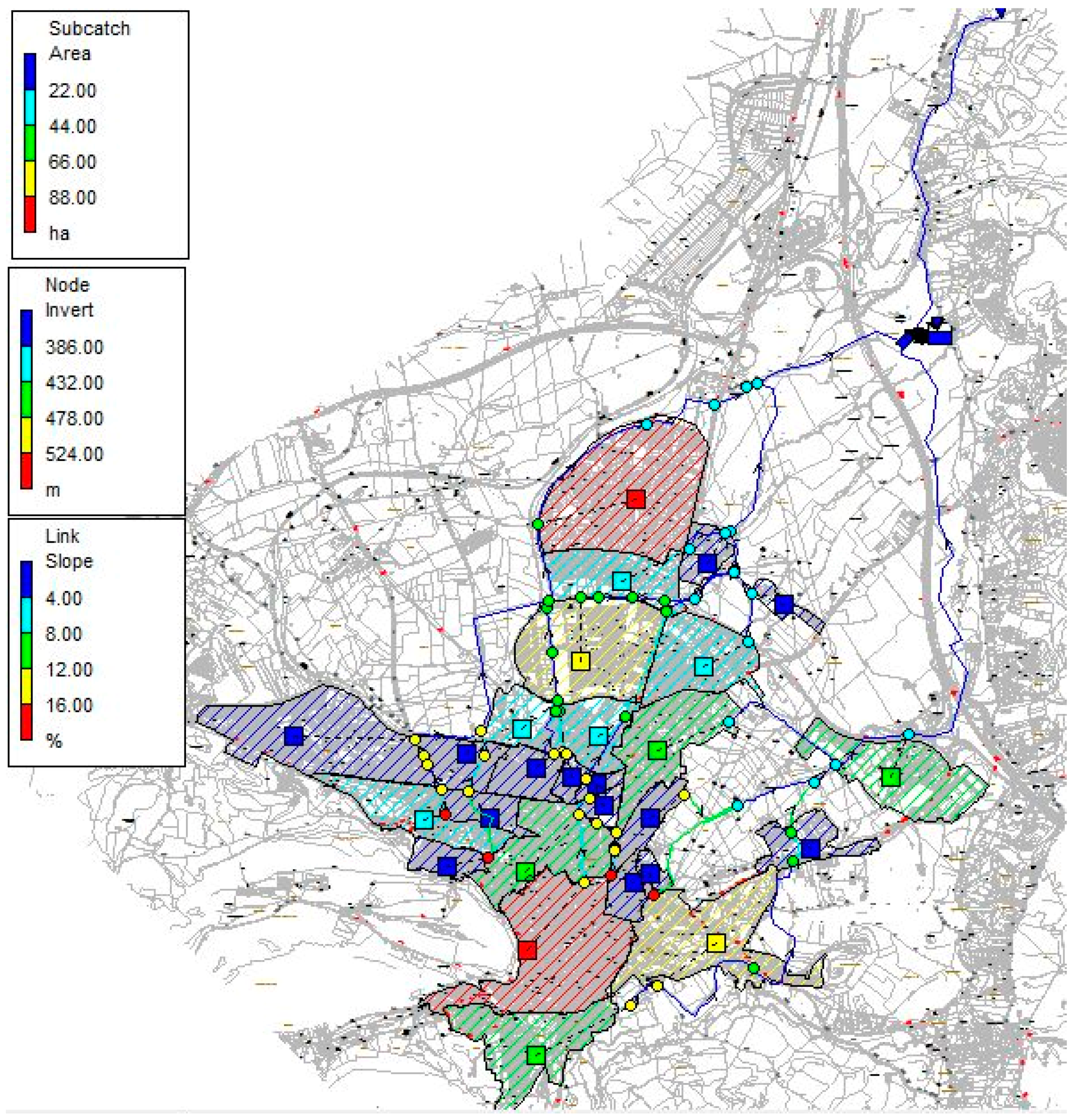
Graphical information of the study area is also provided in Figure 1.
The main features of the studied catchment are shown in Table 3.
In Table 3, Imp Surf. is the Impermeable Surface of the catchment, dp-perv and dp-imp are the maximum levels of depression storage of pervious and impervious areas respectively, and nperv and nimp are the corresponding Manning coefficients.
Regarding the maximum depression storage coefficient, the reference values from the SWMM user manual (2005) [23] and Rossman (2015) [22] were applied. The assumption that pervious areas are similar to “Pasture”, in most cases, undeveloped surfaces within urban areas, was adopted. The Manning coefficients for surface runoff were taken from reference values indicated in GMMF (2005) [23] and Rossman (2015) [22], and impervious surfaces were deemed to be equivalent to “smooth asphalt”, whereas permeable surfaces were considered to be similar to “range (natural)”.
On the other hand, flow routing (water flow through sewer pipes represented in SWMM), is governed by the momentum and the conservation of mass equations (i.e., the Saint Venant equations). These equations were solved by applying the dynamic wave routing method. In addition, the water depth within pipes was estimated using the Manning equation. Meanwhile, infiltration was modelled through the Soil Conservation Service (SCS) Curve Number method.
Overflow pollution was calculated with reference to the mass and concentration of the total suspended solids (TSS), since they are strictly correlated with other common urban pollutants (such as Biochemical Oxygen Demand in five days (BOD5), Chemical Oxygen Demand (COD), and heavy metals), as shown, for example, by Gupta and Saul (1996) [14]. Hogland et al. (1984) [24] also reported that a large proportion of other pollutants, such as nutrients, heavy metals, COD, and organic compounds, may be associated with the presence of sewer solids in wastewater through adsorption/absorption processes. They concluded that up to 90% of the total phosphorus and organic matter (COD) discharged via stormflow may originate from resuspended pipe deposits. Other authors [25] have shown that the variation in suspended solids, chemical oxygen demand, and orthophosphates, follows a similar pattern, whilst Verbanck et al. (1994) [26] confirmed that heavy metals and organic pollutants are primarily associated with the finest particulates. Sartor and Boyd (1972) [27] obtained a clear correlation between the TSS concentration and other pollution parameters (BOD5, COD, and heavy metals). Consequently, in this paper, TSS was used to quantify discharged pollution.
The power function described by Rossman (2015) [22] was, accordingly, used to model the accumulation (B) of TSS (mass per unit area):
where t is the preceding dry weather, C1 is the maximum possible build-up (mass per unit area), C2 is the build-up rate constant (day−1), and C3 is the time exponent. Furthermore, pollutant wash-off occurs during wet weather periods, and is described through exponential wash-off, which was also described by Rossman (2015) [22], as follows:
where W is the wash-off load in units of mass per hour, E1 is the wash-off coefficient, E2 is the wash-off exponent, q is the runoff rate per unit area (mm/h), and B is the TSS build-up (mass per unit area).
In order to establish the above coefficients, the values applied by Hossain et al. (2010) [28] and displayed in Table 4 were used.
Numerical simulations can be performed with design hyetographs obtained from either particular episodes of rain or from any other procedure that generates synthetic hyetographs [16].
Calibrating SWMM model parameters is an intensive task because of both the size and complexity of the studied catchment. Accordingly, in order to carry out this calibration process, Barco et al. (2008) [29], used a geographic information system (GIS) to process the input data and generate the spatial distribution of precipitation. In addition, the complex method was applied to estimate runoff parameters. The parameters that were shown to be the most sensitive to the impervious surface and the depression storage of impervious areas, and least sensitive to the Manning coefficient, were used in the model.
The above research could have been applied to calibrate our SWMM model. However, as the necessary information for the development of a GIS was unavailable, the bibliography was used to determine the value of the parameters of the SWMM model. In this paper, a procedure was used to obtain design hyetographs from IDF curves. Although it could be applied using any IDF curve, the simple model proposed by Témez (1978) [30], which uses the intensity of rainfall, duration of rainfall, and return period, was used here. This model also takes the geographical situation of the system into account.
where It (mm/h) is the average rainfall intensity corresponding to the interval of duration t; Id (mm/h) is the daily average rainfall intensity corresponding to the return period considered (Id = Pd/24); Pd (mm) is the maximum daily rainfall corresponding to the return period considered; I1 (mm/h) is the hourly rainfall intensity corresponding to the return period considered. The value of the parameter I1/Id depends on the site; a value of I1/Id = 9 is considered here. t (h) is the duration of the interval to which It relates.
By applying the above expression for durations of between 1 and 24 h, an intensity level was obtained for each duration value and, from this, the amount of rainfall was determined. The intensity value for each time interval was then obtained as the difference between the rainfall during a storm’s duration at the beginning of the interval minus the rainfall during a storm’s duration until the previous interval. Thus, the intensity at hour 5, for example, would represent the rainfall of a 5 h storm (I5·5), minus the rainfall of a 4 h storm (I4·4). In this way, starting from the Témez (1978) [30] model, the hourly temporal distribution was obtained.
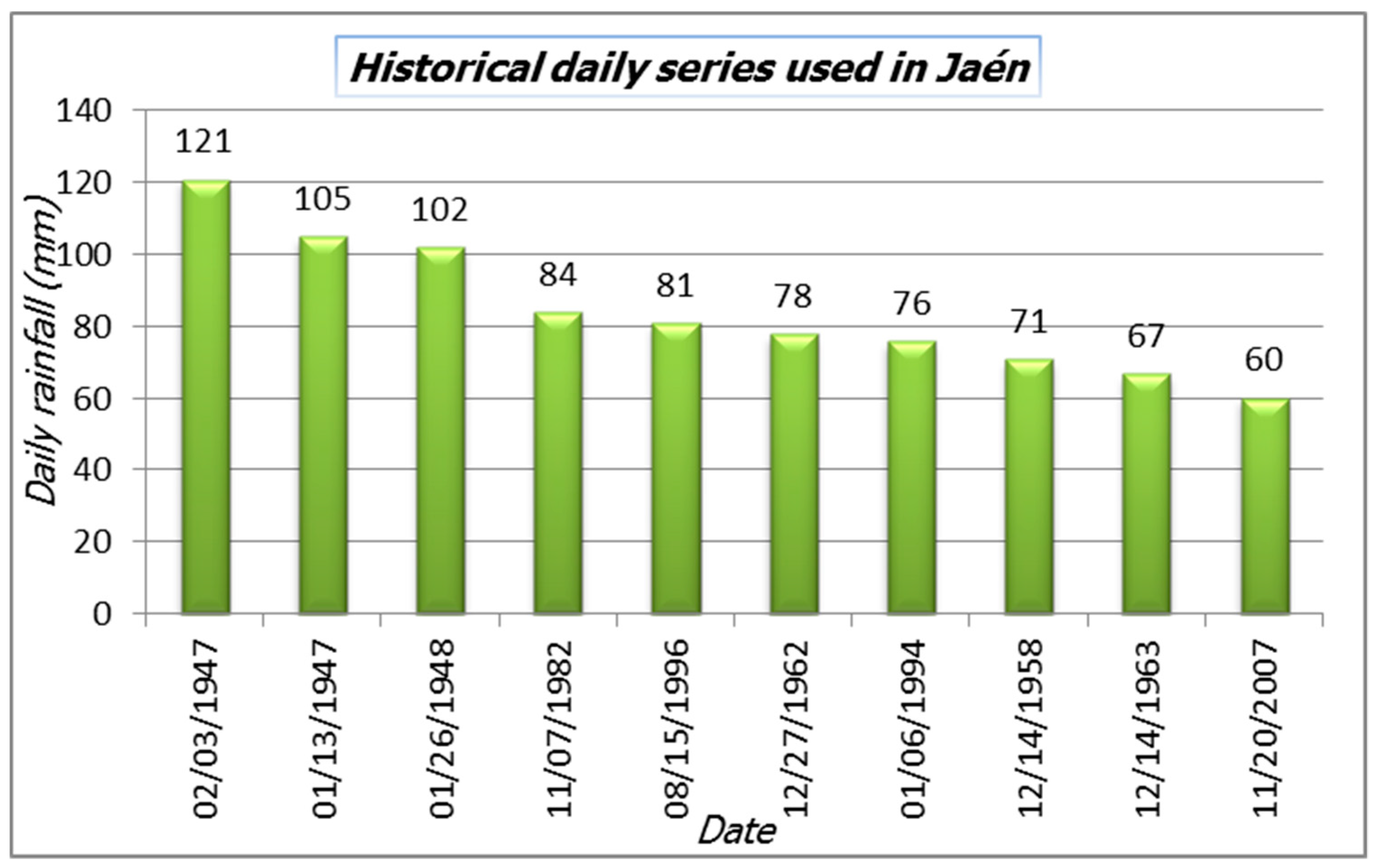
Precipitation time data were requested from the Spanish Meteorological Agency ([20]) at weather station 5270B in Jaén. Figure 2 shows the logs used in the model of Jaén. The logs displayed match the daily rain values, with hourly logs only being available from 2001.
The value of the daily average intensity of rainfall (Id) was subsequently adjusted so that the total daily rainfall corresponded with the registered values. Finally, once the intensity values above 24 h had been estimated, it was possible to reorder them to obtain advanced, delayed, or symmetrical (stepped, centred with alternate hourly steps) hyetographs. It is worth acknowledging that delayed hyetographs (precipitation values sorted in ascending order) produce the least efficient results; this method was selected to define the shape of the storm design.
Simulations were performed on the combined sewer of Jaén according to the common typology of Spanish sewer systems. Calculations for the sanitary flow in the combined sewer were performed by assuming an average dry weather flow, Qdw, obtained through the adoption of a total allocation of 250 litres per inhabitant per day. According to current practice in Spanish sewer systems, the maximum flow conveyed to the treatment plant (Qm) was assumed to be Qm = 5 Qdw. Given that an ideal divider was assumed in the simulations, a constant cut-off flow was considered as the inflow varied.
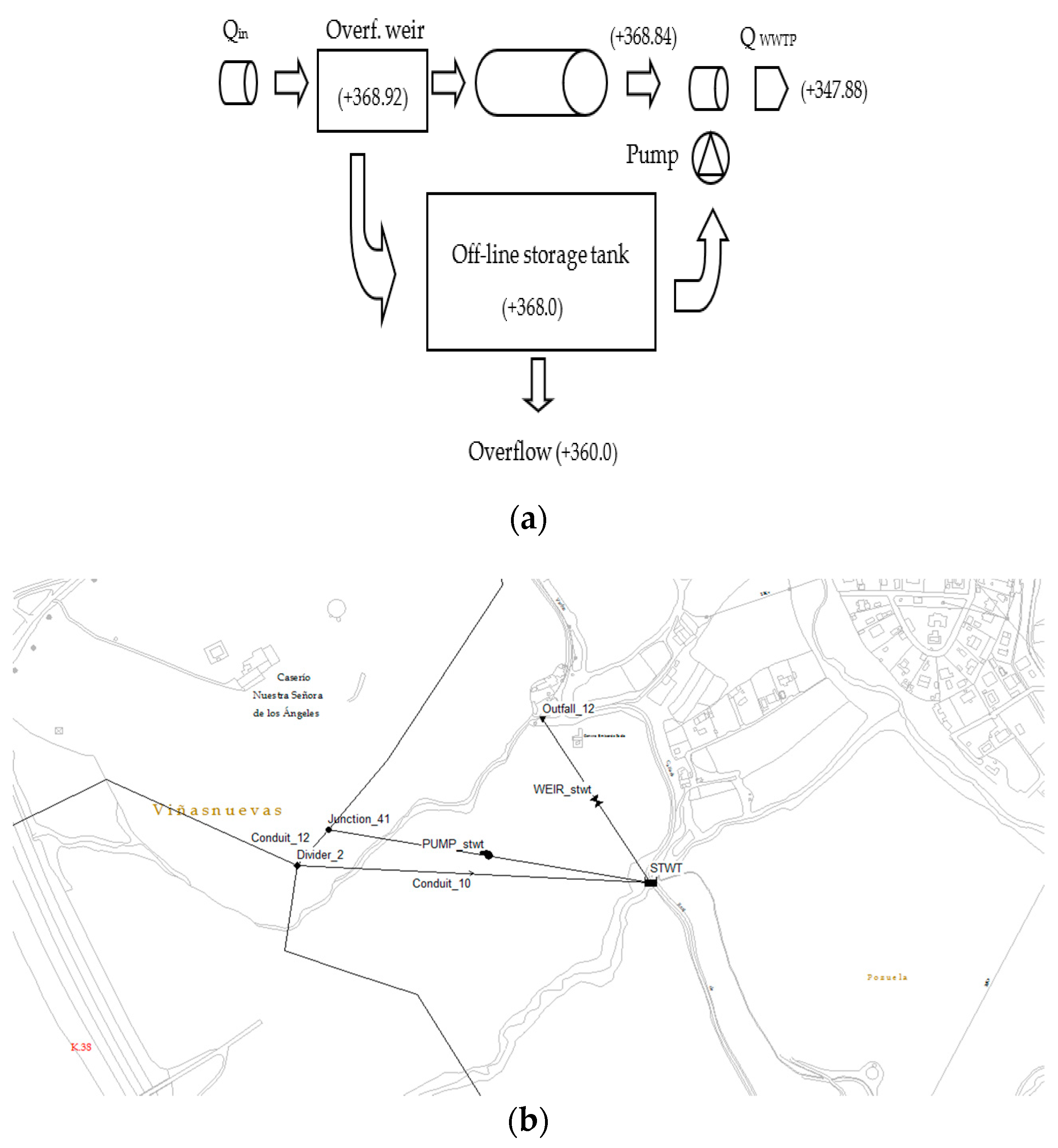
In this paper, the performance of an offline storage tank was analysed. To do this, an ideal facility was provided just upstream of the current WWTP, as shown in the upper right corner of Figure 1. The tank volume ranged with the impervious surface of the catchment (impervious hectare, haimp) from 0 m3/haimp to 100 m3/haimp, and it was assumed that there was a perfect combination of pollutants in the tank at every time step. The operating scheme of the stormwater tank is sketched in Figure 3.
An offline tank starts filling when the inflow discharge exceeds the divider cut-off flow (Cc × Qdw, Cc coefficient of proportionality). When the tank is full, a weir diverts the excess discharge into the receiver. The tank is drained by means of a pumping system after the rainfall has ceased, and the wastewater is conveyed to the treatment plant. The pumping flow for the stormwater sewer is Cc × Qdw. Given that the maximum wastewater flow conveyed to the treatment plant is Cc × Qdw, and the peak hourly coefficient for sanitary flow for the combined sewer is approximately 2, the pumping flow draining the tank is (Cc − 2) × Qdw.
In order to compare the different design configurations and operating conditions of stormwater detention tanks (SWDTs), Todeschini et al. (2012) [5] described the performance indexes (PIs) that can be applied, inter alia, to individual events, as follows:
- The maximum concentration of pollutants in the overflow;
- The duration of overflow/the duration of stormwater runoff;
- The pollutant mass captured/the pollutant mass in the stormwater runoff;
- The volume sent to the wastewater treatment plant/the volume of stormwater runoff;
- The SWDT emptying time.
Calabrò and Viviani (2006) [9] evaluated the behaviour of detention tanks using similar PIs, namely, the efficiency (calculated as the ratio between the total mass of TSS entrapped in the tank and the total mass washed off during a single event), number, duration, concentration, flow, and mass discharge. Furthermore, Anta et al. (2007) [31] estimated the effect of the size of online and offline tanks while considering both the number of CSO events and the percentage of spilled runoff.
In our research, in order to evaluate the responses of sewer systems to different storms, the following efficiency indices, described by De Martino et al. [11] and [12], were determined:
The pollution load removal rate, η, is defined as
where Mr is the TSS mass flowing into the receiver and Mc is the total mass accumulated in the catchment.
The receiver overflow rate, θ, is defined as
where Wr is the water volume discharged into the receiver, and Wc is the total rainfall volume in the catchment. Low values of η and high values of θ implicate that a greater water mass and volume is being transferred to the receiver, thereby leading to a more unfavourable operation of the sewer systems.
3. Results
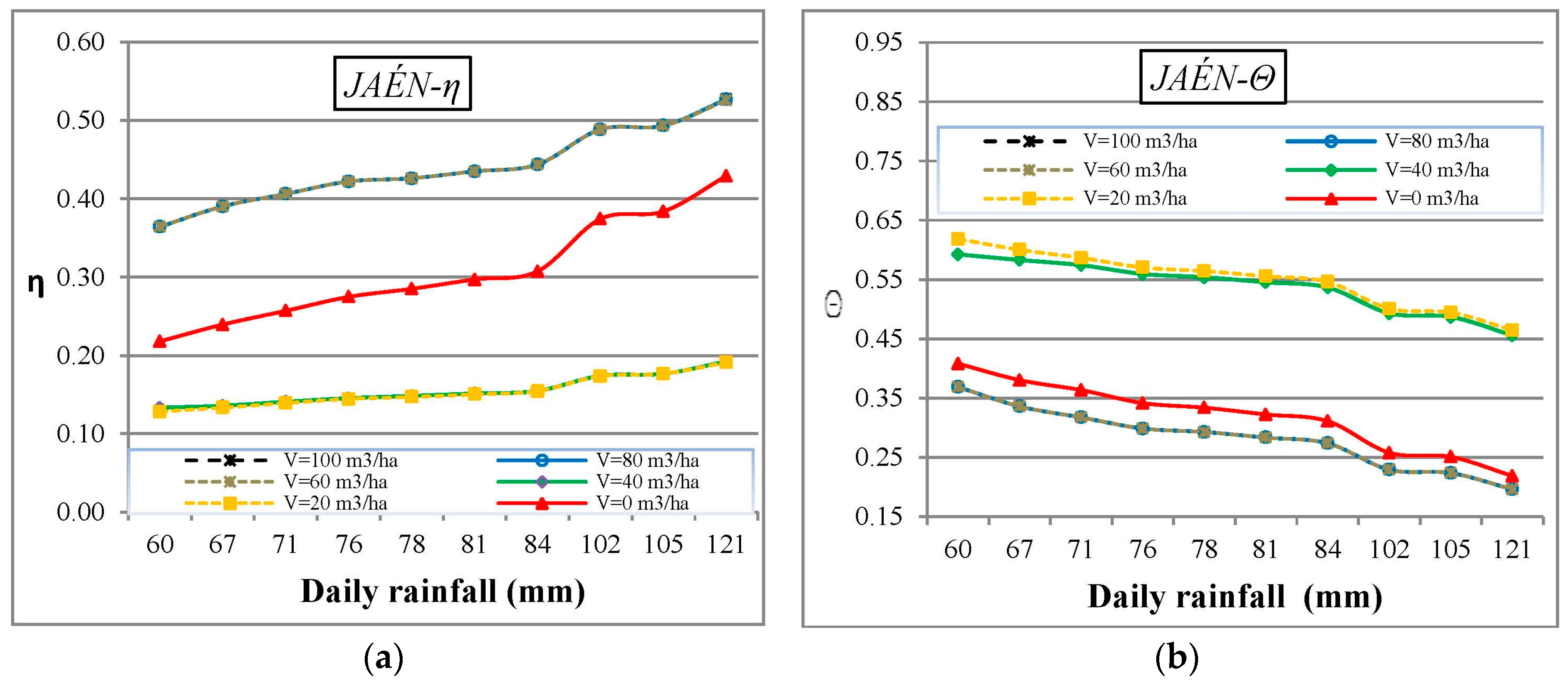
In the simulations, the tank volume (V) varied from 0 m3/haimp to 100 m3/haimp. The values of η and θ were calculated with previously developed equations for offline tanks, where V increases in segments of 20 m3/haimp.
The obtained values are shown in Figure 4, where the efficiency indices are grouped in the form of discrete functions for each volume of the tank.
It can be seen that Jaén’s system is more efficient in terms of pollution reduction with higher levels of rainfall. Furthermore, for different tank volumes, the level of efficiency in Jaén had a certain degree of variability, so the relationship between the extreme values was ηmáx/ηmín = 4.10 and θmáx/θmín = 3.15. In addition, as the pollution load removal rate, η, increased, the receiver overflow rate, θ, slightly decreased with the level of rainfall.
Proposed Methodology
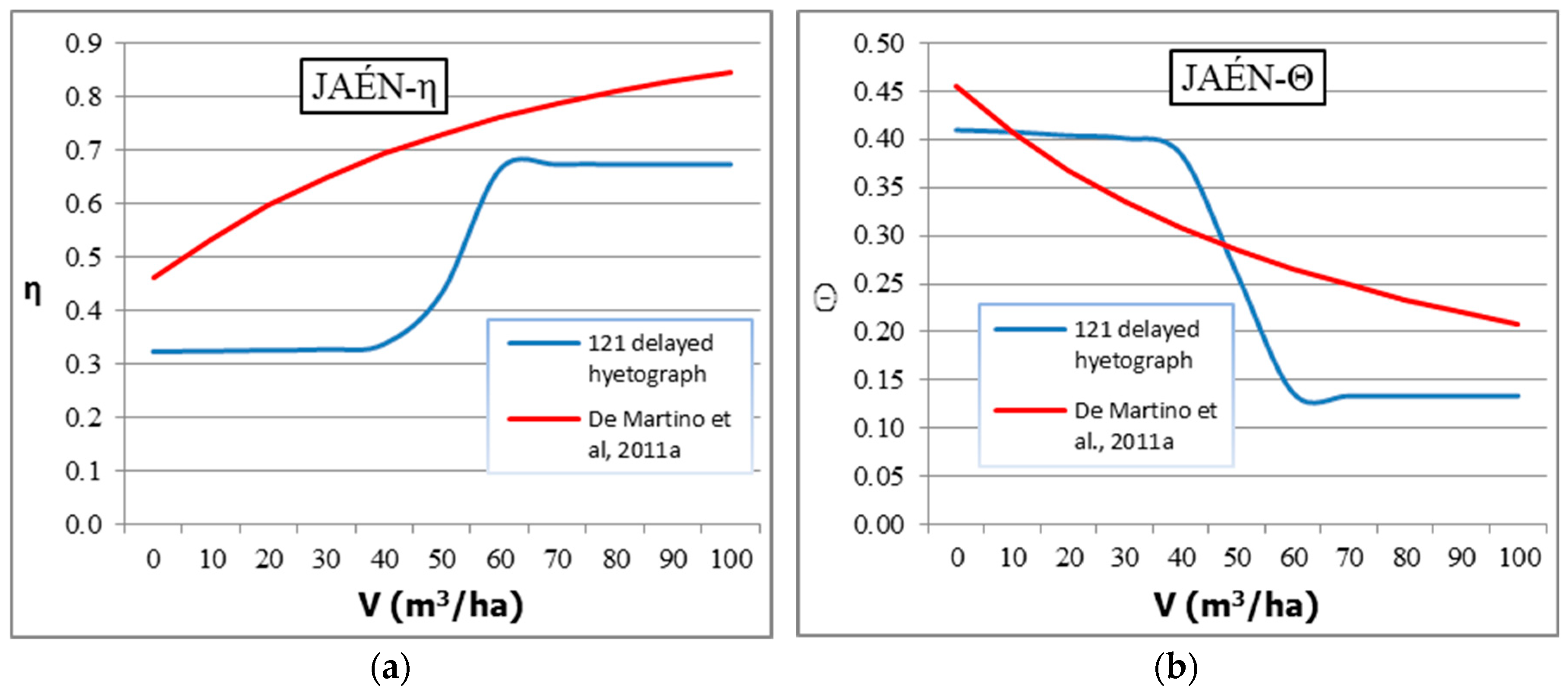
The results of the research developed by De Martino et al. [11] and [12] in the Italian regions of Campania, Umbria, and Piemonte were tested. These studies showed that rainfall regime has a limited influence on the pollutant load and discharge flow into a receiver. In addition, De Martino et al. (2011b) [12] determined the average curves applied to offline stormwater tanks when the cut-off flow of the sewer overflow was set to 5·Qdw as follows:
Figure 5 compares previous average curves with the results obtained in the SWMM model of Jaén, using the historical maximum episode (121 mm on 3 February 1947) with delayed distribution (121 delayed hyetograph).
As shown in Figure 5, a threshold value exists for the tank volume of close to 60 m3/ha; after this, no efficiency improvements were achieved.
The finding of this value prompted us to propose a simple storm tank sizing methodology, based on the search for the threshold values of the efficiency indices. This proposal consisted of determining the efficiency indices η and θ (for example, through a SWMM model) by varying the volume of the tank. The optimal sizing volume was determined to be the value from which the mentioned indexes did not experience significant variation.
4. Discussion
Validation of Results
When sizing stormwater tanks, the ATV A 128 standard [32] is commonly applied, not only in Germany and Spain, but in most European countries. Accordingly, in order to compare and contrast the results obtained, this regulation was applied to our study location. The values of the parameters used are summarised in Table 5.
The results shown in Table 6 resulted in a specific storage volume close to the value of 60 m3/ha.
The value of 60 m3/ha obtained through the proposed methodology matches with that obtained with the implementation of the ATV A 128 standard.
In addition, the results are in accordance with the conclusions drawn from Anta et al. (2007) [31], where differences among the cities of Lugo, Santander, and Santiago de Compostela were used to estimate the magnitude of the volume required in the design of stormwater tanks. According to Anta et al. (2007) [31], if the idea is to produce overflows roughly 20 to 30 times per year, the storage volume will vary between 20 and 90 m3/ha, assuming that the discharge sent to the WWTP is 5–7 times greater than the mean discharge. If the objective is instead to retain 90% of the annual runoff, the storage volume will vary between 35 and 90 m3/ha.
Thus, it was verified that the proposed volume for the storm tank coincides both with current regulations and with other research works. However, these results still need to be compared with field data. In addition, this proposal was made just for a single, specific location within the Mediterranean Basin. In order to expand the application area of the present proposal, the scope of our research should be extended to diverse locations of the Mediterranean Basin.
5. Conclusions
The development of a numerical model in a real and specific drainage system located in the Mediterranean Basin of the Iberian Peninsula facilitated the evaluation of the efficiency of the control measures used to improve the quality parameters of receiving water bodies. The spatial variability of the Mediterranean climate renders it impossible to apply the conclusions drawn from several prior research studies. These studies proposed the use of simple regression equations to estimate both the pollution load removal rate and the receiver overflow rate. Such equations were reviewed, and it was found that the values they obtained were very different from those obtained in the SWMM model presented here. In the absence of a calibration model, the observed differences were over 200% (see Figure 5).
Previous studies have used drainage systems within a small virtual urban catchment (areas measuring around 4 ha in contrast with 1000 ha in Jaén), in addition to distinctive local rainfall patterns. Certainly, the average rainfall per wet day in previous studies showed values between 7.3 and 15.1 mm, in contrast with historical maximum episodes (121 mm in Jaén). According to the results obtained in our investigated drainage system, a threshold value can be identified for the tank volume, above which the system’s efficiency does not substantially improve. This leads us to recommend the threshold value as the design volume of the stormwater tank. This volume would be around 60 m3/ha in Jaén, a value that is in accordance with the conclusions drawn by Anta et al. (2007) [31]. Furthermore, the specific volume obtained after the application of the ATV A 128 [32] standard closely corresponds with that previously indicated in Jaén.
This raises the possibility that the procedure used here could be just as applicable to stormwater tanks located in the Mediterranean Basin. However, it is necessary to compare these results with field data. Moreover, in order to expand the application area of the present research, it is important to focus future studies on specific Mediterranean sites in the Iberian Peninsula and investigate both the characteristics of their drainage systems and their specific rainfall regimes, with the aim of investigating models that could work effectively for all types of basins and sewer systems, regardless of their unique attributes.
Author Contributions
M.J.G.-R. and F.O. conceived and designed the experiments; M.H. performed the experiments and simulations; M.J.G.-R., F.O. and M.H. analysed the data; M.H. and M.J.G.-R. wrote the paper.
Funding
This research did not receive funding external to the University of Granada, Spain.
Acknowledgments
The authors wish to express their sincere thanks to the reviewers for their valuable and constructive suggestions.
Conflicts of Interest
The authors declare no conflict of interest.
References
- Salaverría, M. Las Redes Unitarias de Saneamiento: Criterios de Diseño y Control. 1995. Available online: http://hispagua.cedex.es/documentacion/articulo/58505 (accessed on 23 February 2018).
- Osorio, F.; García, P.; Hontoria, E. Técnicas y Gestión de Las Aguas Pluviales; Universidad de Granada: Granada, Spain, 2012; ISBN 97884-15418-86-3. [Google Scholar]
- Barco, J.; Papiri, S.; Stenstrom, M.K. First flush in a combined sewer system. Chemosphere 2008, 71, 827–833. [Google Scholar] [CrossRef] [PubMed]
- Duan, H.-F.; Li, F.; Yan, H. Multi-objective optimal design of detention tanks in the urban stormwater drainage system: LID implementation and analysis. Water Resour. Manag. 2016, 30, 4635–4648. [Google Scholar] [CrossRef]
- Todeschini, S.; Papiri, S.; Ciaponi, C. Performance of stormwater detention tanks for urban drainage systems in northern Italy. Environ. Manag. 2012, 101, 33–45. [Google Scholar] [CrossRef] [PubMed]
- Itsukushima, R.; Ogahara, Y.; Iwanaga, Y.; Sato, T. Investigating the influence of various stormwater runoff control facilities on runoff control efficiency in a small catchment area. Sustainability 2018, 10, 407. [Google Scholar] [CrossRef]
- United States Environmental Protection Agency. Methodology for Analysis of Detention Basins for Control of Urban Runoff Quality; United States Environmental Protection Agency: Washington, DC, USA, 1986.
- De Paola, F.; De Martino, F. Stormwater tank performance: Design and management criteria for capture tanks using a continuous simulation and a semi-probabilistic analytical approach. Water 2013, 5, 1699–1711. [Google Scholar] [CrossRef]
- Calabrò, P.; Viviani, G. Simulation of the operation of detention tanks. Water Res. 2006, 40, 83–90. [Google Scholar] [CrossRef] [PubMed]
- Oliveri, E.; Viviani, G.; La Loggia, G. Comportamento ed efficienza delle vasche di pioggia. Atti della II Conferenza Nazionale sul Drenaggio Urbano 2001, 279–290. (In Italian) [Google Scholar]
- De Martino, G.; De Paola, F.; Fontana, N.; Marini, G.; Ranucci, A. Pollution Reduction in Receivers: Stormwater Tanks. J. Urban Plan. Dev. 2011, 137, 29–38. [Google Scholar]
- De Martino, G.; De Paola, F.; Fontana, N.; Marini, G.; Ranucci, A. Preliminary design of combined sewer overflows and storm water tanks in southern Italy. Irrig. Drain. 2011, 60, 544–555. [Google Scholar] [CrossRef]
- Huebner, M.; Geiger, W.F. Characterization of the performance of an off line storage tank. Water Sci. Technol. 1996, 34, 25–32. [Google Scholar] [CrossRef]
- Gupta, K.; Saul, A.J. Specific relationships for the first flush load in combined sewer flows. Water Res. 1996, 30, 1244–1252. [Google Scholar] [CrossRef]
- Guo, J.C.Y.; Urbonas, R.B. Runoff capture and delivery curves for stormwater quality control designs. J. Water Resour. Plan. Manag. 2002, 128, 208–215. [Google Scholar] [CrossRef]
- Pochwat, K.; Słyś, D.; Kordana, S. The temporal variability of a rainfall synthetic hyetograph for the dimensioning of stormwater retention tanks in small urban catchments. J. Hydrol. 2017, 549, 501–511. [Google Scholar] [CrossRef]
- Bolle, H.-J. Mediterranean Climate: Variability and Trends (Regional Climate Studies); Springer: Berlin, Germany, 2003; ISBN 3540438386. [Google Scholar]
- Goossens, C. Principal component analysis of Mediterranean rainfall. J. Climatol. 1985, 5, 379–388. [Google Scholar] [CrossRef]
- Köppen, W. Versuch einer klassifikation der klimate, vorzugsweise nach ihren Beziehungen zur Pflanzenwelt. Geogr. Zeitschrift 1900, 6, 593–611. [Google Scholar]
- Agencia Estatal de Meteorología. Guía Resumida del Clima en España (1981–2010). 2012. Available online: http://www.aemet.es/en/conocermas/recursos_en_linea/publicaciones_y_estudios/publicaciones/detalles/guia_resumida_2010 (accessed on 23 February 2018).
- Granata, F.; Gargano, R.; de Marinis, G. Support vector regression for rainfall-runoff modeling in urban drainage: A comparison with the EPA’s storm water management model. Water 2016, 8, 69. [Google Scholar] [CrossRef]
- Rossman, L.A.; Water Supply and Water Resources Division; Office of Research and Development. Storm Water Management Model. User’s Manual Version 5.1; United States Environmental Protection Agency: Washington, DC, USA, 2015.
- Grupo Multidisciplinar de Modelación de Fluidos. GMMF-SWMM Modelo de Gestión de Aguas Pluviales 5.0 vE: Manual del Usuario; Universidad Politécnica de Valencia: Valencia, Spain, 2005. [Google Scholar]
- Hogland, W.; Berndtsson, R.; Larson, M. Estimation of quality and pollution load of combined sewer overflow discharge. Göteborg 1984, 841–850. [Google Scholar]
- Lessard, P.; Beron., C.; Briere, F. Estimation of water quality in combined sewers: The Montreal experience. In Proceedings of the 1st International Seminar on Urban Drainage Systems; Southampton, UK, 1982; pp. 367–375. [Google Scholar]
- Verbanck, M.A.; Ashley, R.M.; Bachoc, A. International Workshop on the origin, occurrence and behavior of sediments in sewer systems: Summary of conclusions. Water Res. 1994, 28, 187–194. [Google Scholar] [CrossRef]
- Sartor, J.; Boyd, G. Water Pollution Aspects of Street Surface Contamination; United States Environmental Protection Agency: Washington, DC, USA, 1972. [Google Scholar]
- Hossain, I.; Imteaz, M.; Gato-Trinidad, S.; Shanableh, A. Development of a catchment water quality model for continuous simulations of pollutants build-up and wash-off. Int. J. Environ. Chem. Ecol. Geol. Geophys. Eng. 2010, 37, 941–948. [Google Scholar]
- Barco, J.; Wong, K.M.; Stenstrom, M.K. Automatic Calibration of the U.S.EPA SWMM Model for a large urban catchment. J. Hydraul. Eng. 2008, 134, 466–474. [Google Scholar] [CrossRef]
- Témez, J.R. Cálculo Hidrometeorológico de Caudales Máximos en Pequeñas Cuencas Naturales. 1978. Available online: https://www.fomento.es/recursos_mfom/0610400.pdf (accessed on 23 February 2018).
- Anta, J.; Beneyto, M.; Cagiao, J.; Temprano, J.; Piñeiro, J.; González, J.; Suárez, J. Analysis of combined sewer overflow spill frequency/volume in north of Spain. Int. Assoc. Hydraul. Eng. Res. 2007, 32, 458. [Google Scholar]
- Abwasser Technische Verein (ATV). Standards for the Dimensioning and Design of Stormwater Structures in Combined Sewers. 1992. Available online: https://www.dwa.de/dwa/shop/produkte.nsf/4C8CE159B0F5CA13C125753C00334F59/$file/vorschau_ATV-A_128E.pdf (accessed on 23 February 2018).
Figure 1.
Non-scaled image of the study area.

Figure 2.
Historical daily series of rainfall in Jaén.

Figure 3.
(a) Scheme of the offline storage tank (combined sewer); (b) Screenshot of the tank implemented into the SWMM model (Qin: inlet flow to the system; QWWTP: inflow to the Waste Water Treatment Plant).
Figure 3.
(a) Scheme of the offline storage tank (combined sewer); (b) Screenshot of the tank implemented into the SWMM model (Qin: inlet flow to the system; QWWTP: inflow to the Waste Water Treatment Plant).

Figure 4.
(a) Pollution load removal rate, η, obtained from the SWMM model of Jaén; (b) receiver overflow rate, , using maximum daily rainfall values, P, and as the volume of the offline tank, V, varied.
Figure 4.
(a) Pollution load removal rate, η, obtained from the SWMM model of Jaén; (b) receiver overflow rate, , using maximum daily rainfall values, P, and as the volume of the offline tank, V, varied.

Figure 5.
(a) The pollution load removal rate, η, in Jaén compared with the average curves obtained in De Martino et al. (2011a) [11]; (b) the receiver overflow rate, θ, in Jaén, compared with the average curves obtained in De Martino et al. (2011a) [11].

Table 1.
Average monthly number of significant (signif.) and stormy rainfall days in Jaén [20].
Table 1.
Average monthly number of significant (signif.) and stormy rainfall days in Jaén [20].
| Jan | Feb | Mar | Apr | May | Jun | Jul | Aug | Sep | Oct | Nov | Dec | Total | |
|---|---|---|---|---|---|---|---|---|---|---|---|---|---|
| signif. | 8.8 | 8.1 | 7.1 | 9.4 | 7.8 | 3 | 0.7 | 1.3 | 4.5 | 8 | 9.6 | 10.3 | 78.6 |
| stormy | 0.1 | 0.1 | 0.2 | 0.5 | 0.9 | 0.9 | 0.3 | 0.5 | 1 | 0.5 | 0.1 | 0.3 | 5.4 |
Table 2.
Features of the storm water management model (SWMM) developed for Jaén.
| Variable | Jaén |
|---|---|
| Number of subcatchments | 27 |
| Subcatchment area (ha) | 1000 |
| Number of nodes | 61 |
| Number of links | 60 |
| Total length of links (m) | 32,632 |
| Number of land uses | 2 |
Table 3.
Studied catchment parameters.
| Area (Ha) | Width (m) | Slope (%) | Imp Surf. (%) | nimp | nperv | dp-imp (mm) | dp-perv (mm) |
|---|---|---|---|---|---|---|---|
| 1000 | 13,218 | 2.53% | 73% | 0.011 | 0.130 | 2 | 5 |
Table 4.
Build-up and wash-off parameters used (Hossain et al. 2010) ([28]).
Table 4.
Build-up and wash-off parameters used (Hossain et al. 2010) ([28]).
| Impervious Surface | Pervious Surface | |
|---|---|---|
| C1 | 60 kg/ha | 30 kg/ha |
| C2 | 26 kg/ha | 8 kg/ha |
| C3 | 0.16 | 0.16 |
| E1 | 0.10 | 0.07 |
| E2 | 0.15 | 0.05 |
Table 5.
Parameters used during the application of the ATV A 128 standard.
| Hydrological | |
| Ai: impervious area (ha) | 729.91 |
| Ig: average slope of drained area | 2.679 |
| tc: concentration time (h) | 4.29 |
| Z: impermeability coefficient of the basin | 0.70 |
| hpr: annual rainfall (mm) | 493 |
| JT: mean terrain slope | 0.025 |
| I: design population (inhab) | 111,401 |
| ws: daily average water provision (L/inhab/day) | 250 |
| Qd24: dry weather flow in daily average (L/s) | 322.34 |
| Qc24: commercial wastewater flow (L/s) | 18.92 |
| Qi24: industrial wastewater flow (L/s) | 120.58 |
| Qiw24: sewer infiltration water flow (L/s) | 0.00 |
| Qcw: combined wastewater discharge to the sewage treatment plant (L/s) | 2449.29 |
| x: Number of hours per day with grey water consumption (h) | 8 |
| ac: number of hours per day of commerce work (h) | 12 |
| ai: number of hours per day of industry work (h) | 16 |
| bc: number of days of business work (days) | 300 |
| bi: number of days of industry work (days) | 312 |
| Pollution | |
| w: annual COD load in the basin (kg/ha) | 280.32 |
| Cd24: COD concentration in local domestic wastewater (mg/L) | 600.00 |
| Cc24: COD concentration in local commercial wastewater (mg/L) | 600.00 |
| Ci24: COD concentration in local industrial wastewater (mg/L) | 600.00 |
| Ctp: average COD concentration in the effluent from the WWTP (mg/L) | 70.00 |
| Cdw: dry weather concentration (mg/L) | 600.00 |
| Cr: average COD concentration in runoff waters (mg/L) | 107.00 |
Table 6.
Results of applying the ATV A 128 standard.
| Results of Applying the ATV A 128 Standard | |
|---|---|
| m: mean mix ratio in overflow water | 16.64 |
| Cr: average COD concentration in runoff water (mg/L) | 81.23 |
| Cd: average COD concentration in dry weather flow (mg/L) | 1229.42 |
| e0: permissible annual overflow rate (%) | 14.72 |
| VS_ATV: specific storage volume (m3/ha net) | 59.67 |
© 2018 by the authors. Licensee MDPI, Basel, Switzerland. This article is an open access article distributed under the terms and conditions of the Creative Commons Attribution (CC BY) license (http://creativecommons.org/licenses/by/4.0/).
Share and Cite
MDPI and ACS Style
Hermoso, M.; García-Ruiz, M.J.; Osorio, F. Efficiency of Flood Control Measures in a Sewer System Located in the Mediterranean Basin. Water 2018, 10, 1437. https://doi.org/10.3390/w10101437
AMA Style
Hermoso M, García-Ruiz MJ, Osorio F. Efficiency of Flood Control Measures in a Sewer System Located in the Mediterranean Basin. Water. 2018; 10(10):1437. https://doi.org/10.3390/w10101437
Chicago/Turabian StyleHermoso, Martín, María Jesús García-Ruiz, and Francisco Osorio. 2018. "Efficiency of Flood Control Measures in a Sewer System Located in the Mediterranean Basin" Water 10, no. 10: 1437. https://doi.org/10.3390/w10101437
Note that from the first issue of 2016, this journal uses article numbers instead of page numbers. See further details here.