Solitary Wave Generation and Propagation under Hypergravity Fields

Institute of Systems Engineering, China Academy of Engineering Physics, Mianyang 621900, China
*
Author to whom correspondence should be addressed.
Water 2018, 10(10), 1381; https://doi.org/10.3390/w10101381
Submission received: 22 July 2018
/
Revised: 28 September 2018
/
Accepted: 28 September 2018
/
Published: 2 October 2018
(This article belongs to the Special Issue Applications of Computational Fluid Dynamics for Marine and Offshore Engineering)
Abstract
:The traditional small-scale marine engineering experiments that are performed under normal gravity fields always encounter one stubborn difficulty related to full-scale prototype models. However, the difficulty can be resolved by centrifuge experiments that can generate hypergravity fields in which the centrifuge acceleration is many times greater than the gravity acceleration. In this study, the generation of solitary waves in hypergravity fields is proposed using solitary wavemaker theory and scaling laws. A series of case simulations are performed under four different gravity fields (1 g, 30 g, 50 g, and 100 g, where g is the gravity acceleration). These cases are presented and discussed in detail to understand and verify the scaling laws and the stability of the solitary wave during its generation and propagation within hypergravity fields. The numerical results show that the waveform and the static pressure field that are obtained during the simulations performed under different gravity fields agree well at the macroscale. Since the velocity field is sensitive to wave attenuation, time lag, fluid viscosity and surface tension, some discrepancies can be found in the velocity field. It should be noted that the fluid viscosity and surface tension have influence on the wave attenuation. However, wave attenuation and time lag can be offset by a well-designed incident wave condition.
1. Introduction
Coupled with the scarcity of land, population growth has led to the widespread overexploitation of the coasts and oceans. Moreover, extreme climate changes have led to the more frequent occurrence of extreme disastrous events, including storms and tsunamis [1]. Consequently, ocean engineering and coastal engineering services are becoming increasingly necessary in severe environments due to overexploitation and extreme meteorological and hydrological conditions. However, the quantification of such new conditions remains to be explored, and current design codes still rely upon the use of approximate and unverified empirical formulas without details of the wave-structure interaction process or analogous processes that must be considered [2]. Therefore, there is a significant demand for further research to address these topics and update the currently considered design codes and construction approaches to ensure the reliability and durability of the structures serviced under extreme meteorological and hydrological conditions. For this purpose, a series of studies have been performed on a variety of topics, including simulations of tsunami propagation in the Pacific Ocean and its impacts on the coastal regions of China [3,4], tsunami-induced sediment transport [5], on-bottom stability analysis of cylinders under solitary waves [6], long wave and shelf interactions [7,8,9,10,11,12,13] and flooding-building interactions [14]. Nevertheless, there is an inherent difficulty in such studies in that the scale of the engineering involved tends to be massive, while prototype or full-scale experiments are difficult (if not impossible) to construct in most cases and are rather costly. For this reason, small-scale models are always used in practice for the study of wave-structure interactions or other analogous processes. However, because of the scale effect, self-weight stresses and gravity-dependent processes, which are frequent in ocean engineering and coastal engineering, cannot be properly reproduced by small-scale models, in which the self-weight stresses are very small compared with those of a prototype. Furthermore, it should be noted that the stress-strain behavior of soils is nonlinear, and therefore, the behavior of a downscaled model may not appropriately represent the soil behavior of its prototype. As a consequence, despite their enormous cost, large-scale experiments and prototype-scale experiments are in significant demand [15,16,17].
Nevertheless, self-weight stresses and gravity-dependent processes can be reproduced properly in a small-scale model with the use of a centrifuge, which can produce a hypergravity field in which the centrifugal acceleration is many times greater than the acceleration due to gravity; as a result, the behaviors of the prototype-scale models can be properly studied [18]. Hypergravity fields generated within a centrifuge are often labeled N g, where N is the ratio of the centrifugal acceleration to the gravity acceleration. Hence, centrifuge experiments are frequently used in the laboratory to study the actual behaviors of prototype models. For example, Brennan et al. [19] studied the strength reduction in the upheaval buckling of buried pipes, Baziar et al. [20] investigated the responses of underground tunnels to rupture reverse faults, and Candia et al. [21] discussed the response of a retaining wall to seismic activity. In addition, centrifuge experiments have been developed to study water-soil interactions (e.g., the research on submarine landslides presented by Coulter and Phillips [22], Coulter [23], and Gue [24]). Meanwhile, wave tanks have been constructed within centrifuge devices to facilitate research on the wave-induced liquefaction of sand beds [25,26,27].
However, at present, centrifuge experiments are considered solely for geotechnical engineering, particularly because water wave problems, which constitute the basic focus of ocean engineering, cannot currently be properly reproduced within a centrifuge. In addition, few individuals have conducted research on water wave problems using centrifuge experiments; this is likely attributable to the widespread reliance upon wave tanks to study natural phenomena such as wave reflection [28], wave generation [11,29,30,31], and wave-structure interactions [7,8,9,10,11,12,13,14,15,16,17,32,33]. Unfortunately, wave tanks cannot be properly constructed within a centrifuge due to their shape and scale. Although Sekiguchi [25] and Sassa [26,27] created wave tanks within centrifuges, such tanks can be used only to study geological phenomena, because the low-quality wave fields generated within relatively short wave tanks are unable to meet the requirements of most ocean engineering experiments. Therefore, there is a significant demand for research on the generation and propagation of water waves in hypergravity fields.
Solitary wave, which is a type of long wave, has been used for decades to study the behaviors of tsunamis because of the similarities in their wave hydrodynamics [10]. In addition, the interactions between solitary waves and coastlines have drawn considerable attention with respect to various wave processes, including wave disintegration, run-up, and transmission. In the present paper, the generation and propagation of solitary waves onto a shelf in a shallow-water wave tank under different gravity fields are numerically simulated. To verify the effectiveness of the numerical wave generation and propagation simulations, the results are compared with reported experiments, wavemaker theory and the numerical results that are generated under different gravity fields. The piston-type wavemaker, which been used by many other researchers in both physical wave tanks and numerical simulations of wave tanks [9,34], is considered for the generation of solitary waves because of its high efficiency in shallow-water environments [34]. In addition, dynamic mesh technology is utilized in this study to simulate the motion of the piston-type wavemaker. The unsteady, two-dimensional, Reynolds-averaged Navier-Stokes (RANS) equations are solved in conjunction with both the Renormalization Group (RNG) k-ε model used for treating the turbulence and the volume-of-fluid (VOF) method for tracking the free surface.
2. General Scaling Laws
The self-weight stresses and gravity-dependent processes involved in coastal, ocean and geological engineering cannot be properly reproduced under normal gravity fields; therefore, the observations derived from small-scale models cannot be related to observations from full-scale prototypes. However, the centrifuge represents a powerful tool that can be used to reproduce the behavior of a prototype at a small scale, because the magnitude of the produced centrifugal acceleration is many times greater than the Earth’s gravity. The scaling laws for centrifuge modeling are shown in Table 1, where n is defined as the ratio of the model length to the prototype length, L is the length, T is the time, and M is the mass. In this study, the same fluid is considered.
As shown in Table 1, the model scaling that is considered for the kinematic viscosity coefficient is N1/2n3/2, which indicates that the viscosity cannot be scaled unless n is defined as N−1/3. With this scale, gravity similarity and viscosity similarity can coincide simultaneously. However, when n is considered to be N−1/3, the model is not a small-scale model; on the contrary, it is a large-scale model. In addition, experiments on large-scale models such as wave-structure interactions cannot be performed in a centrifuge. Therefore, although gravity similarity and viscosity similarity can simultaneously coincide in a hypergravity field, viscosity similarity is ignored in this paper. This is similar to experiments performed under normal gravity fields, because both the generation and the propagation of waves are processes that are dependent upon the gravity field and the model scale. In fact, in a centrifuge model test, the centrifuge acceleration is always labeled as N times the gravity acceleration (hereinafter referred to as N g, where g is the gravity acceleration). 1/N is always defined as the model scaling factor to ensure that the centrifuge acceleration is identical to the prototype acceleration. With these scaling laws, the model scaling factors for the wave celerity and fluid field static pressure are both one, which means that the dynamic and static pressures in a small-scale model are equal to the pressures in a full-scale model. Therefore, the self-weight stresses and gravity-dependent processes can be appropriately reproduced. For this reason, the above-mentioned scaling laws are considered in this study. Additionally, the discrepancies between the simulation results and the theoretical results due to viscosity and surface tension are discussed in this paper.
3. Wave Generation
Solitary wave is a type of long wave that exhibits an approximately permanent form during its generation and propagation process. The water particle velocity of a long wave is approximately constant with respect to the water depth. Based on this characteristic, Goring derived a formula to determine the wave paddle trajectory for the generation of a solitary wave by a piston-type wavemaker [7] in which the average horizontal velocity of the water particles adjacent to the wavemaker is assumed to be equal to the wave paddle velocity:
where ξ is the position of the piston at a time t, t is the elapsed time since the start of the wave generation, c is the wave celerity, d is the still water depth, and η is the free surface displacement. In addition, based on the Boussinesq solitary wave solution, the free surface displacement η can be described as:
where H is the solitary wave height, and kwn is the wave number that is determined as:
Although in theory a solitary wave has an infinite wavelength, Goring [7] recommended that the wavelength l be calculated by:
This wavelength is chosen because the amplitude of a solitary wave is zero for η/H < 0.001. The wavelength is used in this study for estimating the Reynolds (Re) number, which can be used for estimating the turbulent kinetic energy, turbulent dissipation rate, and y+.
Furthermore, the wave celerity c is determined as:
Substituting Equation (2) into Equation (1), the piston trajectory that is required to generate a solitary wave can be described as:
Referring to the solitary wave generation theory developed by Goring [7], the piston stroke S can be calculated as:
and the duration of paddle motion τ can be approximately described as:
Nevertheless, the wave generation theory presented above is applicable only to the generation of solitary waves under a 1 g gravity field (i.e., the normal gravity field). For solitary wave generation under an N g gravity field, Equation (5) should be expanded to:
Then, with the above-presented scaling laws, this equation can be rewritten as:
It is clear that the model scaling for the wave celerity is in accordance with the scaling laws that are shown in Table 1. The wave number kwn, the piston stroke S, the wavelength l, and the duration of paddle motion are successively described as:
and:
All of the above-mentioned features of solitary waves, such as the wave celerity, wave number, piston stroke, wavelength and duration of paddle motion, are in accordance with the scaling laws listed in Table 1. In the present paper, a series of solitary wave cases with the scaling laws presented herein are studied both to verify the effectiveness of the scaling laws and understand the generation and propagation of solitary waves in hypergravity fields.
4. Governing Equations and Boundary Conditions
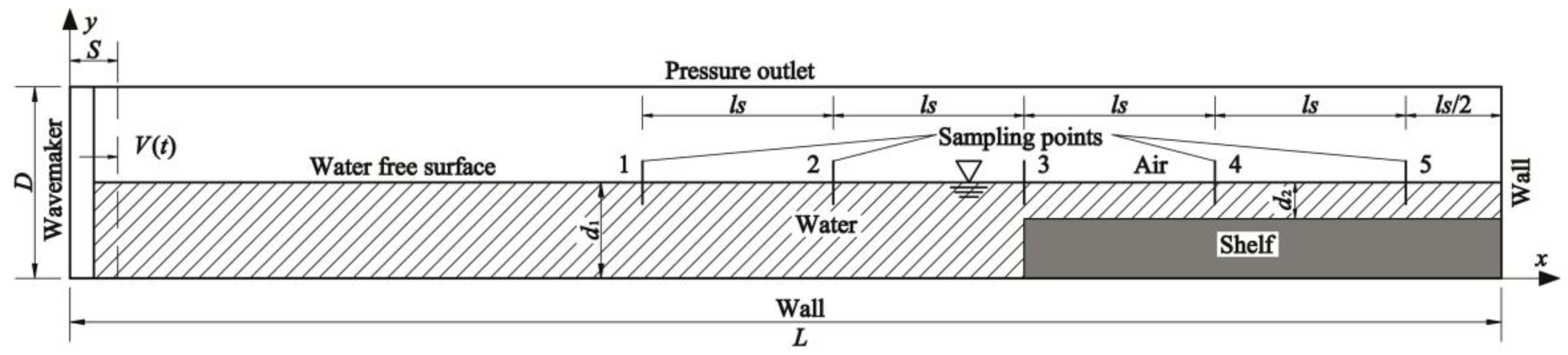
A sketch of the computational model and the boundary conditions considered in this study is shown in Figure 1, which shows that the computational domain is a rectangle (L × D) with a rectangular shelf at the far end of the wave tank opposite from the piston-type wavemaker, which is positioned at the left end of the wave tank. In the simulation, the piston-type wavemaker is forced to move according to a prescribed motion as defined by Equation (6). Five sampling points located in the numerical wave tank are used to obtain the values of the wave profile during the simulation. A brief description of the model used to simulate the solitary wave cases is described hereafter.
4.1. Governing Equations
The governing equations for fluid flow that are used in this study are the two-dimensional RANS equations:
where u and u′ are the mean velocity and fluctuating velocity components, respectively, ρ is the fluid density, P is the pressure, μ is the dynamic viscosity, fi denotes the body forces, and represents the Reynolds stresses, which must be modeled to close the RANS equations. In this study, the RNG k-ε two-equation model is used to solve the Reynolds stresses and close the equations, and it is defined as:
Equations (17) and (18) represent k and ε transport equations for the turbulent kinetic energy and turbulent dissipation rate, respectively. In these equations, the quantities αk and αε are the inverse effective Prandtl numbers for k and ε, respectively, while μeff is the effective viscosity, Gk represents the generation of turbulent kinetic energy due to the mean velocity gradients, and C1ε = 1.42 and C2ε = 1.68 are constants. Rε is defined as:
where Cμ = 0.0845, η0 = 4.38, and β = 0.012 are constant, and ηε is defined as Sεk/ε.
Since the VOF method can model two or more immiscible fluids by solving a single set of momentum equations and tracking the volume fraction of each of the fluids throughout the domain, it is used in this paper for tracking the free surface. The liquid volume fraction equation is defined as:
The field defined by f is a scalar field that propagates according to:
With the liquid volume fraction equation, the variables such as pressure and the density of the mixture phase mesh can be calculated. The iso-surface of the volume fraction equal to 0.5 is the free surface.
4.2. Initial and Boundary Conditions
In this study, the initial condition is a still water body with zero velocity and no surface waves. As shown in Figure 1, an outlet boundary condition with atmospheric pressure is considered at the top of the computational domain. No-slip conditions for the velocity components are imposed on the left, right and bottom boundaries of the computational domain. In addition, the left boundary is considered the wavemaker’s paddle, which is forced to move according to Equation (6) during the simulation. The shelf is modeled as a solid object without any deformation during the simulation. Furthermore, a no-slip condition for the velocity components is imposed at the interface between the shelf and the fluid; this is displayed in Figure 1.
4.3. Numerical Method
The finite volume method (FVM) is considered to solve the governing equations, and the semi-implicit method for pressure-linked equations (SIMPLE) algorithm [35,36] is utilized to enforce mass conservation and obtain the pressure field. PRESTO! [36] is used for the discretization of the pressure; the second-order upwind scheme [37] is used for the discretization of the momentum, turbulent kinetic energy, and turbulent dissipation rate; and the geometric reconstruction scheme [38] is utilized to solve the liquid volume fraction equation. The time marching scheme is first-order implicit. A layering scheme is used for simulating the moving wall, because it can add or remove layers of cells adjacent to a moving boundary.
5. Results and Discussion
This section provides a discussion of the various aspects of the problems under hypergravity fields associated with the generation and propagation of solitary waves in constant water depth, and the interactions of solitary waves with a shelf with a vertical front face. For this purpose, the typical experimental model presented by Goring [7] is considered. The sketch of the computation domain is shown in Figure 1. For all of the cases performed in this study, the upstream depth is d1, the downstream depth is d2, and a depth ratio (d1/d2) of 2.64, which was used by Goring [7], is considered. The front face of the shelf is vertical, and it is located at the far end of the wave tank opposite from the wavemaker at a distance of (2/3) L away from the wavemaker’s initial position, which is located at x = 0, as shown in Figure 1. During the simulation, a solitary wave is generated by moving the wavemaker according to the trajectory defined by Equation (6). The details of the conditions of the experiments that are performed in this paper are shown in Table 2. The solitary wave heights considered under the normal gravity field are chosen based on the wave height presented by Chen et al. [5]; accordingly, the wave heights that are used under other gravity fields are calculated by scaling laws that are based on the wave height used under the normal gravity field. The relative wave heights that are used in this study are 0.2, 0.3, and 0.34, which are within the range of the relative wave height used by Chen et al. [5] and Hsiao et al. [10]. The hypergravity considered in this study are 30 g, 50 g, and 100 g, which represent common centrifuge test cases. The 30 g and 50 g are commonly used by researchers to study water-soil interactions [23,24,25,26]; meanwhile, the scale of the model under the 100 g can match the circular channels of some drum centrifuges [39] and the experimental module of the centrifuge under construction.
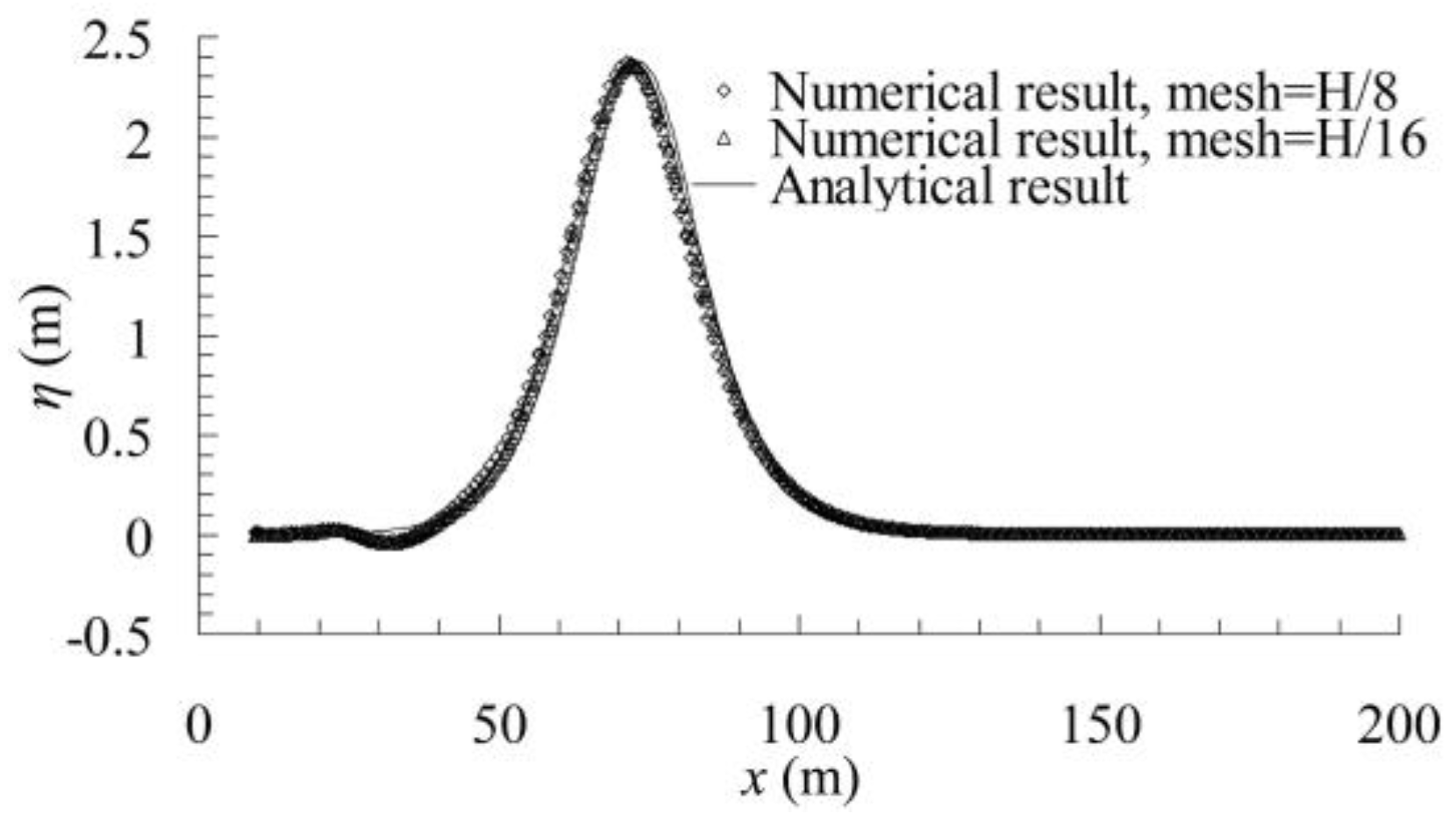
A time step of τ/1000 is found to be sufficiently small to ensure that the results are independent of the time step. To discretize the computational domain, a uniform mesh is adopted. The values of y+ vary a good deal, because the models presented in this paper have very different scales. For cases simulated under the normal gravity field, the values of y+ are approximately 100; for cases simulated under 30 times, 50 times, and 100 times the normal gravity field, the values of y+ are approximately 30, 20, and 10, respectively. It should be noted that the values of y+ have no significant effect on the numerical results, because the effects of the inertia force are much greater than the effects of the viscosity force for the cases that are presented in this study. The mesh size of the other regions is set based on a mesh refinement study in which the mesh size was progressively increased until no significant changes are observed in the results. Two different mesh heights corresponding to H/8 (where H is the solitary wave height) and H/16 are considered. The corresponding mesh width is three times the mesh height. Taking case #013 with maximum wave height as an example, the solitary wave profiles generated using the two mesh sizes are compared with the corresponding Boussinesq analytical results in Figure 2. Good agreement can be seen between the numerical results and analytical results. The good agreement illustrates that the results are independent of the mesh size. Therefore, for the cases in this study, a mesh size of H/8 is considered.
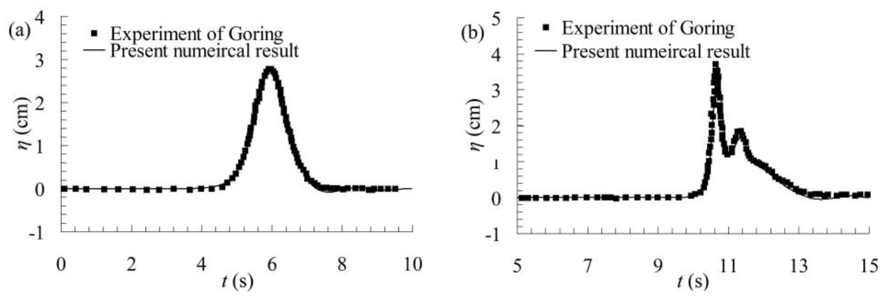
Since similar large-scale experiments performed under normal gravity fields or similar experiments performed under hypergravity fields are rather rare, a similar small-scale experiment presented by Goring [7] is considered to verify the accuracy of the numerical model presented in this paper. In Goring’s experiment, L = 32.5 m, D = 61 cm, the upstream depth d1 is 25 cm, the downstream depth d2 is 9.46 cm, the stroke is 18.25 cm, and the period is 4.24 s. The vertical front face of the shelf is located at a distance of 13 m from the wavemaker’s initial position, sampling point 1 is placed 5.75 m upstream of the step, sampling point 2 is placed at the step, and sampling points 3, 4, and 5 are placed at intervals of 5.68 m downstream of the step, which are slightly different from the model used in this paper. The numerical results from the present paper are compared with the experiments results of Goring [7] in Figure 3. The numerical results agree well with those of the experiments, both at sampling point 2 where the wave propagates over the step, and at sampling point 3, where the wave propagates on the shelf. The good agreement of the results means that the numerical model that is presented in this paper is accurate.
The details and the results of the simulations are provided in the following subsections.
5.1. Solitary Wave Generation and Propagation in a Constant Water Depth
In this subsection, the generation and propagation of solitary waves in a constant water depth within a hypergravity field is presented and discussed. The numerical results of the cases are compared with the analytical results and the numerical results that are displayed under different gravity fields. For this purpose, the Boussinesq solitary wave solution is considered, and the solitary waves are successively displayed under normal gravity, 30 g, 50 g and 100 g. To obtain the wave profile after wave generation and before wave propagation onto the shelf, where the wave propagation occurs in a constant water depth, the section between the wavemaker and the vertical shelf is considered herein.
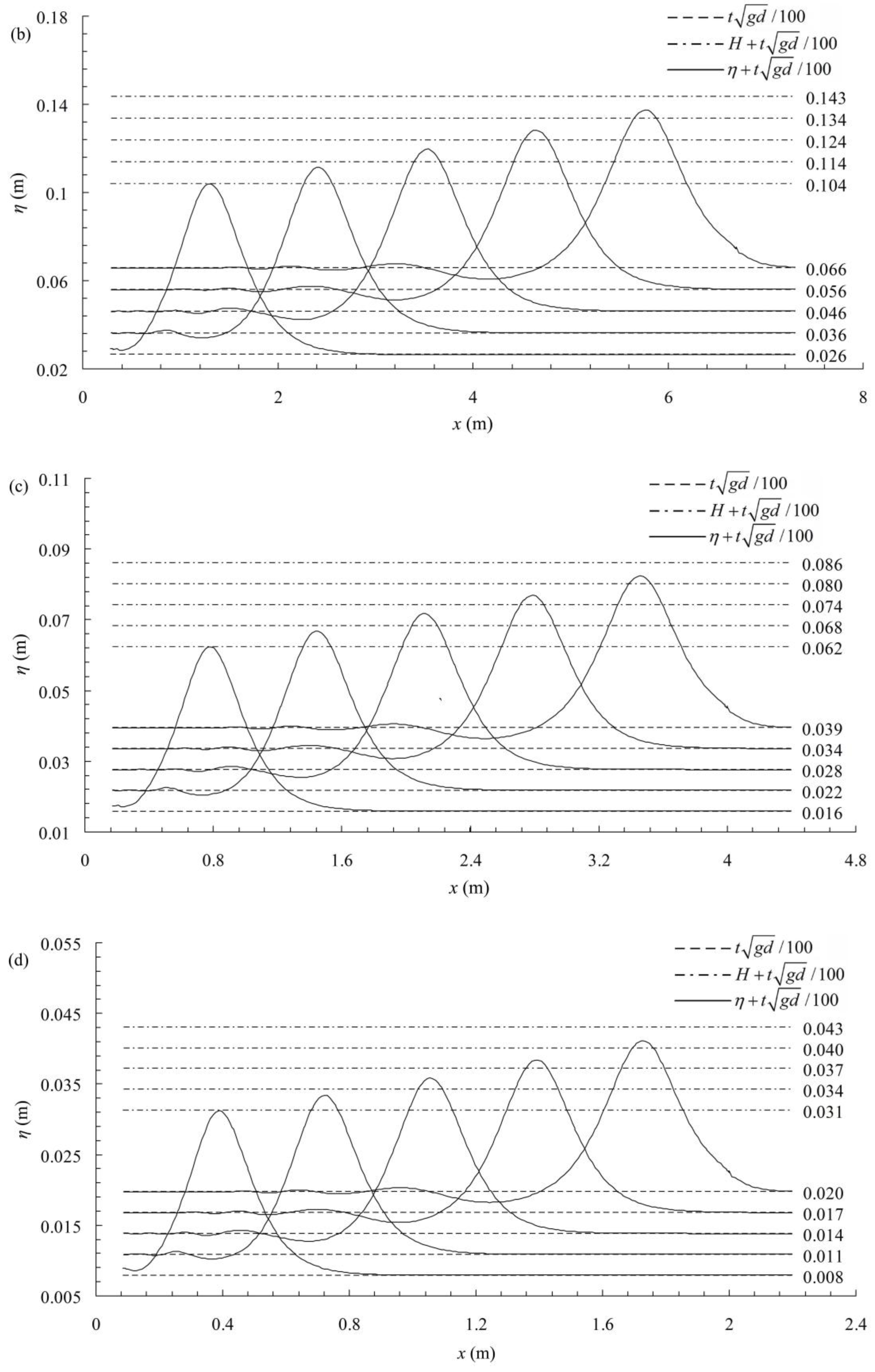
The temporal evolution profiles of the numerical free surface as the wavemaker begins to move at the left end of the wave tank for the cases with maximum relative wave height, namely, cases #013, #303, #503 and #103 in Table 2, are shown in Figure 4; these correspond to dimensionless times of t/τ = 0.8, t/τ = 1.1, t/τ = 1.4, t/τ = 1.7, and t/τ = 2.0, respectively. Due to wave attenuation, the reference wave heights H displayed in the figure are the numerical wave heights at the dimensionless time t/τ = 0.8 for convenient observation. As observed in the figure, the changes in the waveforms are not appreciable. The only difference between the numerical and theoretical results is that the wave height of the solitary wave is slightly smaller than what was defined, especially when the wave has propagated over a longer distance. The differences in the wave heights from the target could have been caused by many reasons, including wavemaker theory [11], wave attenuation, ignored viscosity similarity and surface tension. However, as observed in Figure 4, the discrepancy in the extent of the decline in the wave height among the cases performed under different gravity fields may be caused by the ignored viscosity similarity and surface tension, because the same wavemaker theory is used for all of the cases.
To investigate the scale effect on the wave attenuation, the numerical wave heights in all of the cases tabulated in Table 2 at the five dimensionless times mentioned above are shown in Table 3. The attenuation coefficient εa that is in consideration for both the model scale and the elapsed propagation time is defined as:
where num is the number of the sampling point, h is the reference wave height, hi is the wave height at the sampling point, ti is the elapsed time since the reference time, and N is the scale of the model. The values of the attenuation coefficient εa of the cases are also displayed in Table 3. The reference wave height that was used in Table 3 is the numerical wave height at a dimensionless time of t/τ = 0.8 to avoid the initial instabilities caused by the wave generation. The reference time is 0.8 τ. Cases #011, #301, #501, and #101, which are tabulated in Table 2, are characterized by small wave numbers and long wavelengths. Slight reflection effects are observed at the dimensionless time of t/τ = 2.0, causing the wave height at this time to be slightly larger. Therefore, for these cases, the wave heights at the dimensionless time of t/τ = 2.0 are abandoned. As observed in Table 3, the discrepancies in the wave attenuation among the numerical results for the cases under the same gravity field may be attributed to the highly nonlinear effect caused by a high relative wave height. The discrepancies in the wave attenuation among the numerical results obtained from the simulations under different levels of gravity fields may be attributed to the ignored viscosity similarity, surface tension similarity and other complex reasons. Although the values of the attenuation coefficient displayed in Table 3 with the model scales that were considered do not noticeably vary, the attenuation coefficients for all of the cases performed in this study are less than 1%. The discrepancies in the wave attenuation among the numerical results for the cases with a maximum relative wave height are more appreciable, as shown in Figure 4. It is clear that wave attenuation may be more serious in a small-scale model, and the serious wave attenuation may cause a lower wave height and a more serious time lag. Therefore, it deserves closer attention. In addition, it should be mentioned that the use of Boussinesq’s solution in this paper might exacerbate the wave attenuation phenomenon; in contrast, Grimshaw’s solution and Fenton’s solution may be more exact when the relative wave height is not very high [11].
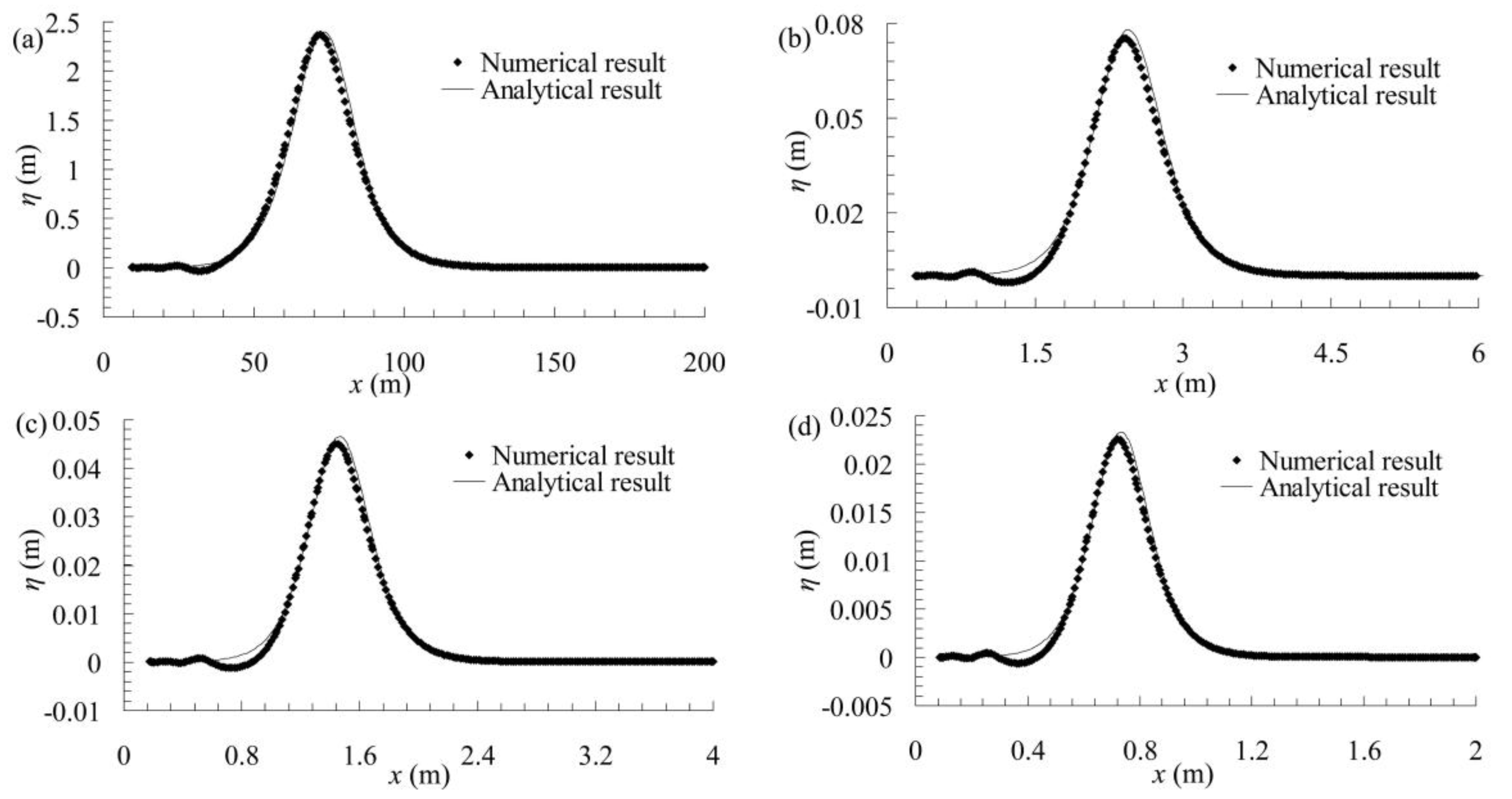
To verify the accuracy of the numerical results, the numerical results and analytical results are compared with each other at a dimensionless time of t/τ = 1.1 for cases with maximum relative wave height (cases #013, #303, #503 and #103 in Table 2). For this purpose, the Boussinesq analytical solution is considered. The solitary wave heights that are used to calculate the analytical results are the numerical wave heights at the dimensionless time of t/τ = 0.8; these reduce the influence of wave attenuation, which can cause the wave height to decrease and the time lag to increase. Due to the discrepancy between the theoretical and numerical wave heights caused by wave attenuation during the propagation of the solitary wave, the numerical wave celerity is smaller than the wave celerity calculated by the theoretical solution shown in Equation (5). In addition, discrepancies between the numerical and theoretical wave celerity can affect the traveling distance. As observed in Figure 5, the numerical results from the present cases agree well with the theoretical results from all of the cases simulated under different gravity fields. However, upon close examination of the wave crest, the wave traveling distance and the trailing oscillatory waves, some discrepancies are detected between the numerical and the analytical results. The discrepancies between the wave crests displayed in Figure 5 could be attributed to wave attenuation, which might be affected by the model scale, as noted above. The discrepancies in the trailing oscillatory waves behind the main wave among the numerical results may have other complex causes, such as surface tension; however, these differences are not significant compared with the main wave, and the trailing oscillatory waves would attenuate quickly, as shown in Figure 4 and Figure 5.
5.2. Solitary Wave Interacting with Shelf
In this subsection, the interactions between solitary waves and an underwater shelf with a vertical front face within a hypergravity field are presented and discussed. The experimental conditions considered in this subsection are tabulated in Table 2. The layout of the numerical wave tank is shown in Figure 1. Five sampling points are located in the numerical wave tank. For cases #013, #303, #503 and #103, which are tabulated in Table 2, the first point is placed upstream from the shelf front face at a distance of 5 D, and the others are placed at intervals of 2.5 D downstream from the first point. For the other cases tabulated in Table 2, the first point is placed upstream from the shelf front face at a distance of 8 D, and the others are placed at intervals of 4 D downstream from the first point. The distance from the fifth (i.e., the last) sampling point to the end wall of the wave tank is ls/2 (as shown in Figure 1); hence, the solitary waves travel a distance of ls between the first and second recorded arrivals at the fifth sampling, after reflecting off the end wall of the wave tank.
A series of events is initiated when a solitary wave propagates onto a shelf. As the wave propagates over the shelf front face, the wave shape changes; eventually, the wave splits into two waves: a reflected wave traveling to the left (i.e., upstream), and a transmitted wave traveling to the right (i.e., downstream). This subsection provides a discussion of the wave propagation after the dimensionless time of t/τ = 2.0 and before the reflected wave, which is generated by the transmitted wave interacting with the end wall of the wave tank, reaching the first sampling point. The dimensionless time t/τ = 2.0 is used as a threshold, because the incident wave (i.e., the initial solitary wave) reaches the shelf front face for most of the cases (as shown in Figure 4) at that time. In particular, for the cases with the maximum wave length (cases #011, #301, #501, and #101 in Table 2), the slight reflection effects generated by the interaction of the initial incident wave with the front face of the shelf are observed at a dimensionless time of t/τ = 2.0.
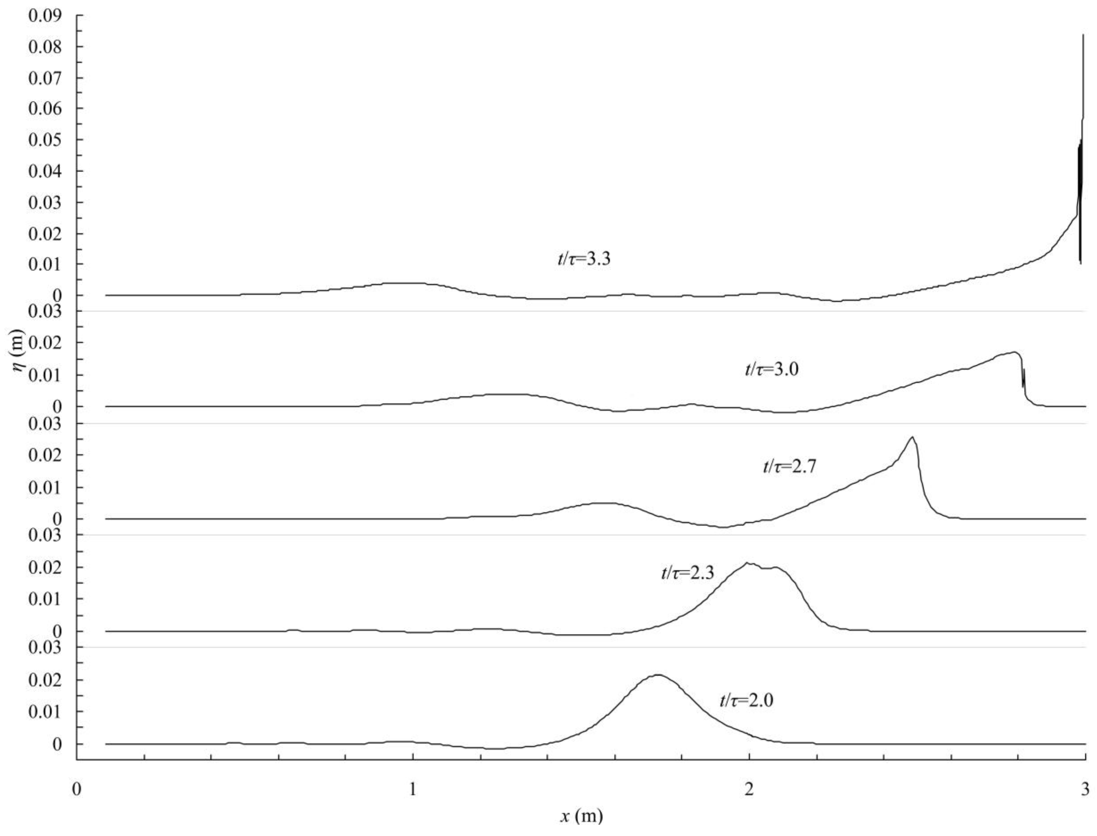
The temporal evolution of the numerical free surface between the dimensionless time t/τ = 2.0 and the dimensionless time t/τ = 3.3, upon which the transmitted wave impacts the end wall of the wave tank for the case with maximum relative wave height and minimum model scale (case #103 in Table 2), is shown in Figure 6. As demonstrated in the figure, many events, including wave shoaling, breaking, impingement and run-up, are observed during the wave propagation onto the shelf. The initial incident wave propagates over the underwater step at about t/τ = 2.3, at which time the wave shape of the initial incident wave changes and begins to split into two waves, as shown in Figure 6. The transmitted wave propagates onto the shelf as the waveform continuously changes, which can be attributed to the wave shoaling. Subsequently, the transmitted wave breaks between t/τ = 2.7 and t/τ = 3.0. Then, between t/τ = 3.0 and t/τ = 3.3, the broken wave impinges and run up onto the end wall of the wave tank. Note that the wave height of the first reflected wave generated by the interaction between the incident wave and the step is too small; as a result, the first reflected wave is not very appreciable in Figure 6.
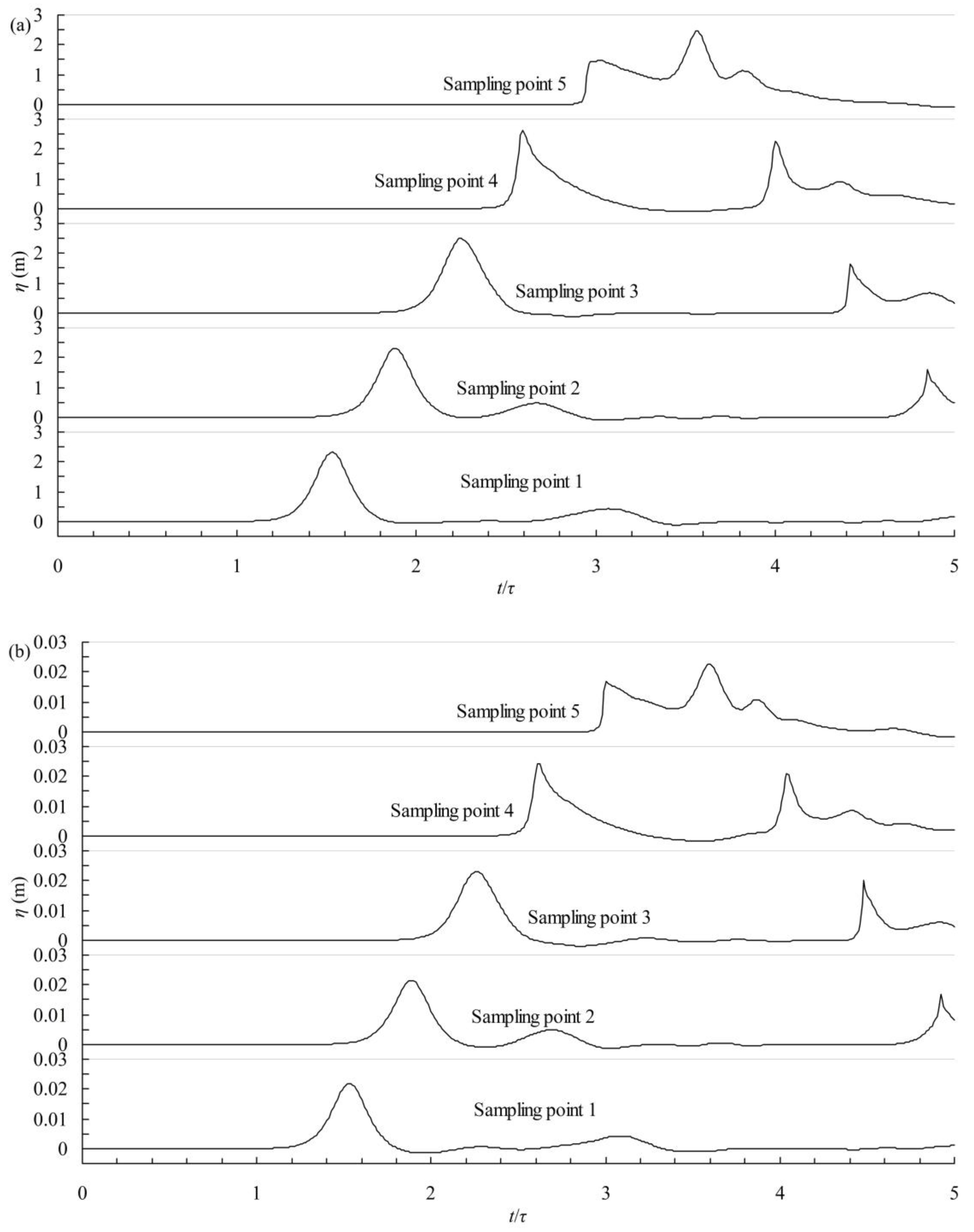
The temporal profiles recorded at the five sampling points during the simulation for the cases with maximum relative wave heights (cases #013 and #103) are shown in Figure 7, from which it is evident that the temporal profiles of the models with different model scales agree well with one another during the propagation of a solitary wave at a constant water depth. The incident wave recorded at sampling points 1 and 2 are approximately symmetric regarding the wave crest, and the trailing oscillatory waves are insignificant and can be disregarded. For case #103, the incident wave heights at sampling points 1 and 2 are 2.19 cm and 2.15 cm, respectively. The discrepancy between the numerical results and the theoretical results can be attributed to wave attenuation, which is more serious in a small-scale model. The first wave height recorded at sampling point 3 (over the step) is 2.31 cm, and it is composed of both the incident and the reflected wave. After the reflection-transmission process, the incident wave splits into two waves: the first reflected wave, which is recorded by sampling points 2 and 1 in succession, and the transmitted wave, which is recorded by sampling points 4 and 5 in succession. However, the waveform and the wave celerity both exhibit some differences during the propagation of the transmitted wave onto the shelf; these differences can be attributed to the discrepancies of wave attenuation and the time lag effect among the various model scales. For example, due to the time lag in case #103, the transmitted wave breaks later. That is why there is a significant difference at sampling point 5, as shown in Figure 7. The velocity fields and the dynamic pressure obtained during the simulations performed under different gravity fields are presented in Section 5.3 for a comparison and a discussion of the wave attenuation, time lag, and influence of the wave field viscosity.
5.3. Comparison of the Simulated Velocity Fields and Dynamic Pressures under Different Gravity Fields
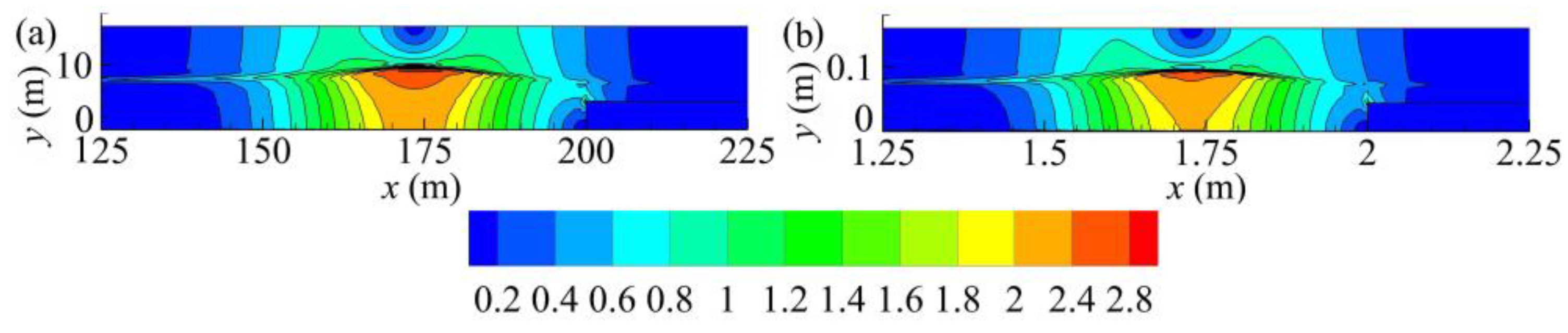
As shown in Section 5.1 and Section 5.2, the waveforms obtained from the simulations performed under different gravity fields agree well with one another. The static pressure that can be calculated by ρg(h+η) also agrees well. In this subsection, the velocity fields and dynamic pressures that may be sensitive to the time lag, wave attenuation and fluid viscosity are presented and discussed. The contours for the cases with maximum relative wave height (cases #013 and #103) that are generated under the normal gravity field and 100 times the normal gravity field are shown for comparison. Two typical dimensionless times during the simulation are considered. The first time is t/τ = 2.0, at which the solitary wave has propagated for a relatively long time, thereby ensuring that the solitary wave has fully developed. Furthermore, at this time, the wave fields are pure, i.e., they are lacking any interference from the reflected wave. The second time is t/τ = 3.0, at which the transmitted wave has propagated on the underwater shelf for a relatively long time.
As observed in Figure 8 and Figure 9, the distributions of the velocity field are similar; however, the magnitudes are different. The magnitude of the velocity field obtained from the downscaled model is smaller than the corresponding velocity field obtained from the prototype, at both time t/τ = 2.0 and time t/τ = 3.0. The discrepancies among the different cases may be caused by time lag, wave attenuation, and the ignored viscosity and surface tension similarity, as mentioned above. In addition, it should be noted that there are two phases in the wave tank: one is the water, and the other is the air. In an experiment, the velocity of the air is always ignored. Therefore, the evolution of the maximum dynamic pressure at sampling point 2 and sampling point 4 for cases #013 and #103 are shown in Figure 10.
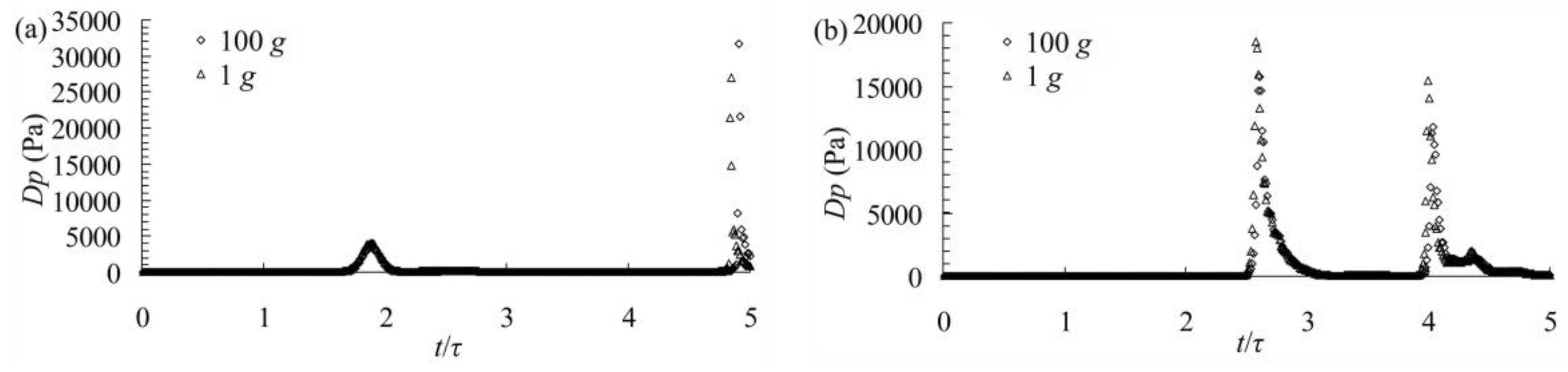
As observed in Figure 10, the dynamic pressure profiles for cases #013 (1 g) and #103 (100 g) agree well most of the time. Only slight differences can be observed at the peaks. At sampling point 2 for case #013, the first peak is 3959 Pa, and the second peak is 26,953 Pa; for case #103, the first peak is 3643 Pa, and the second peak is 31,711Pa. At sampling point 4, for case #013, the first peak is 18,541 Pa, and the second peak is 15,452 Pa; for case #103, the first peak is 15,725 Pa, and the second peak is 11,802 Pa. The maximum difference appears at the second peak at sampling point 4. At sampling point 4 for case #103, the second peak is 24% smaller than that for case #013. At sampling point 2 for case #103, the second peak is 18% larger than that for case #013. The discrepancy between the downscaled model (case #103) and the prototype (case #013) may be attributed to many factors, such as wave attenuation, time lag, fluid viscosity and the surface tension. For sampling point 2 at the first peak, the discrepancy may be mainly caused by wave attenuation, as mentioned in Section 5.1, because more serious wave attenuation may cause a smaller wave celerity as shown in Equation (5). For the other peak values at sampling point 2 and sampling point 4, the discrepancies may be mainly caused by time lag. Since the waveform continuously changes as the wave propagates, the maximum dynamic pressure changes accordingly. Therefore, the discrepancies in the maximum dynamic pressures may be attributed to the wave attenuation and the time lag. The fluid viscosity and surface tension have influence on the wave attenuation, as shown in Table 3, and the time lag may be mainly caused by wave attenuation. However, it should be noted that the discrepancies in the wave attenuation and the time lag can be offset by a well-designed incident wave condition. In addition, the time lag has an influence only on the time and location of the experimental phenomena.
6. Conclusions
In this paper, the solitary wavemaker theory proposed by Goring [7] is expanded for the generation of solitary waves within hypergravity fields in consideration of scaling laws. The typical experimental model presented by Goring [7] is considered. This model is also used in hypergravity fields. A series of case simulations under four different gravity fields are presented and discussed to understand and verify the solitary wave generation theory and the stability of solitary waves during their generation and propagation within hypergravity fields. The accuracy of the numerical results is verified by comparison with the results of wavemaker theory and the results generated under different gravity fields.
The following conclusions can be drawn from this study:
- (1)
- The waveform obtained from the simulations performed under different gravity fields exhibit good agreement at the macroscale, indicating that solitary waves can be steadily generated and propagated within hypergravity fields. Consequently, wave breaking, impingement, run-up, and the other phenomena that have been observed during wave-coasting interactions, which have drawn considerable attention, can be studied using a downscaled model.
- (2)
- Although the waveform and static pressure field agree well at the macroscale, some discrepancies are detected within the details. Due to the ignored viscosity and surface tension similarity, some of the features of solitary waves are affected by the scale effect, including wave attenuation and time lag. Wave attenuation may be more serious in a small-scale model experiment performed within a hypergravity field, and can cause the time lag to become more serious. However, wave attenuation and time lag can be offset by a well-considered incident wave condition.
- (3)
- Since both the velocity and dynamic pressure are sensitive to the wave attenuation, time lag and fluid viscosity, some discrepancies can be found in the velocity field and dynamic pressure profiles. However, a well-designed initial incident wave can weaken the discrepancies in the velocity field and dynamic pressure.
Author Contributions
Q.S.W. and M.H.L. have conceived of and designed the numerical simulations. Q.S.W. has performed the numerical simulation, analyzed the data and written the original paper. D.W.L. has improved the original paper’s language. M.H.L. has supervised the research.
Funding
This research was partly funded by the Centrifugal Hypergravity and Interdisciplinary Experiment Facility (CHIEF), an item of the 13th Five Year National Major Research Infrastructures Plan.
Conflicts of Interest
The authors declare no conflict of interest. The founding sponsors had no role in the design of the study, the collection, analyses or interpretation of data, the writing of the manuscript, or the decision to publish the results.
References
- Kendon, E.J.; Roberts, N.M.; Fowler, H.J.; Roberts, M.J.; Chan, S.C.; Senior, C.A. Heavier summer downpours with climate change revealed by weather forecast resolution model. Nat. Clim. Chang. 2014, 4, 570–576. [Google Scholar] [CrossRef]
- Liang, Q.H.; Chen, K.C.; Hou, J.M.; Xiong, Y.; Wang, G.; Qiang, J. Hydrodynamic modelling of flow impact on structures under extreme flow conditions. J. Hydrodyn. Ser. B 2016, 28, 267–274. [Google Scholar] [CrossRef]
- Ren, Z.Y.; Wang, B.L.; Fan, T.T.; Liu, H. Numerical analysis of impacts of 2011 Japan Tohoku tsunami on China Coast. J. Hydrodyn. Ser. B 2013, 25, 580–590. [Google Scholar] [CrossRef]
- Ren, Z.Y.; Zhao, X.; Wang, B.L.; Dias, F.; Liu, H. Characteristics of wave amplitude and currents in South China Sea induced by a virtual extreme tsunami. J. Hydrodyn. Ser. B 2017, 29, 377–392. [Google Scholar] [CrossRef]
- Chen, J.; Guan, Z.; Jiang, C.B. Study of sediment transport by tsunami waves: V: Influence of mangrove. Adv. Water Sci. 2016, 27, 206–213. [Google Scholar]
- Tripepi, G.; Aristodemo, F.; Veltri, P. On-bottom stability analysis of cylinders under tsunami-like solitary waves. Water 2018, 10, 487. [Google Scholar] [CrossRef]
- Goring, D.G. Tsunamis-the Propagation of Long Waves onto a Shelf; California Institute of Technology: Pasadena, CA, USA, 1979. [Google Scholar]
- Stansby, P.K. Solitary wave run up and overtopping by a semi-implicit finite-volume shallow-water Boussinesq model. J. Hydraul. Res. 2003, 41, 639–647. [Google Scholar] [CrossRef]
- Dong, G.H.; Ma, X.Z.; Perlin, M.; Ma, Y.X.; Yu, B.; Wang, G. Experimental study of long wave generation on sloping bottoms. Coast. Eng. 2009, 56, 82–89. [Google Scholar] [CrossRef]
- Hsiao, S.C.; Lin, T.C. Tsunami-like solitary waves impinging and overtopping an impermeable seawall: Experiment and RANS modeling. Coast. Eng. 2010, 57, 1–18. [Google Scholar] [CrossRef]
- Wu, N.J.; Tsay, T.K.; Chen, Y.Y. Generation of stable solitary waves by a piston-type wave maker. Wave Motion 2014, 51, 240–255. [Google Scholar] [CrossRef]
- Dong, J.; Wang, B.L.; Liu, H. Run-up of non-breaking double solitary waves with equal wave heights on a plane beach. J. Hydrodyn. Ser. B 2014, 26, 939–950. [Google Scholar] [CrossRef]
- Zhao, X.; Wang, B.; Liu, H. Characteristics of tsunami motion and energy budget during runup and rundown processes over a plane beach. Phys. Fluids 2012, 24, 62–107. [Google Scholar] [CrossRef]
- Kelman, I.; Spence, R. An overview of flood actions on buildings. Eng. Geol. 2004, 73, 297–309. [Google Scholar] [CrossRef]
- Masselink, G.; Ruju, A.; Conley, D.; Turner, L.; Ruessink, G.; Matias, A.; Thompson, C.; Castelle, B.; Puleo, J.; Citerone, V.; et al. Large-scale barrier dynamics experiment II (BARDEX II): Experimental design, instrumentation, test program, and data set. Coast. Eng. 2016, 113, 3–18. [Google Scholar] [CrossRef]
- Blenkinsopp, C.E.; Matias, A.; Howe, D.; Castelle, B.; Marieu, V.; Turner, I.L. Wave runup and overwash on a prototype-scale sand barrier. Coast. Eng. 2016, 113, 88–103. [Google Scholar] [CrossRef]
- Matias, A.; Masselink, G.; Castelle, B.; Blenkinsoop, C.E.; Kroon, A. Measurements of morphodynamic and hydrodynamic overwash processes in a large-scale wave flume. Coast. Eng. 2016, 113, 33–46. [Google Scholar] [CrossRef] [Green Version]
- Taylor, R.N. Geotechnical Engineering Technology; Blackie Academic & professional: London, UK, 1995. [Google Scholar]
- Brennan, A.J.; Ghahremani, M.; Brown, M.J. Strength reduction for upheaval buckling of buried pipes in blocky clay backfill. Ocean Eng. 2017, 130, 210–217. [Google Scholar] [CrossRef] [Green Version]
- Baziar, M.H.; Nabizadeh, A.; Mehrabi, R.; Lee, C.J.; Hung, W.Y. Evaluation of underground tunnel response to reverse fault rupture using numerical approach. Soil Dyn. Earthq. Eng. 2016, 83, 1–17. [Google Scholar] [CrossRef]
- Candia, G.; Mikola, R.G.; Sitar, N. Seismic response of retaining walls with cohesive backfill: Centrifuge model studies. Soil Dyn. Earthq. Eng. 2016, 90, 411–419. [Google Scholar] [CrossRef] [Green Version]
- Coulter, S.E.; Phillips, R. Simulating submarine slope instability initiation using centrifuge model testing. In 1st International Symposium on Submarine Mass Movements and Their Consequences; Springer: Dordrecht, The Netherlands, 2003; pp. 29–36. [Google Scholar]
- Coulter, S.E. Seismic Initiation of Submarine Slope Failures Using Physical Modeling in a Geotechnical Centrifuge; Memorial University of Newfoundland: St. John’s, NL, Canada, 2008. [Google Scholar]
- Gue, C.S. Submarine Landslide Flows Simulation through Centrifuge Modelling; University of Cambridge: Cambridge, UK, 2012. [Google Scholar]
- Sekiguchi, H.; Kita, K.; Sassa, S.; Shimamura, T. Generation of progressive fluid waves in a geo-centrifuge. Geotech. Test. J. 1998, 21, 95–101. [Google Scholar]
- Sassa, S.; Sekiguchi, H. Wave-induced liquefaction of beds of sand in a centrifuge. Géotechnique 1999, 49, 621–638. [Google Scholar] [CrossRef]
- Sassa, S.; Sekiguchi, H.; Miyamoto, J. Analysis of progressive liquefaction as a moving-boundary problem. Géotechnique 2001, 51, 847–857. [Google Scholar] [CrossRef]
- Nallayarasu, S.; Fatt, C.H.; Shankar, N.J. Estimation of incident and reflection waves in regular wave experiments. Ocean Eng. 1995, 22, 77–86. [Google Scholar] [CrossRef]
- Ursell, F.; Dean, R.G.; Yu, Y.S. Forced small-amplitude water: A comparison of theory and experiment. J. Fluid Mech. 1960, 7, 33–52. [Google Scholar] [CrossRef]
- Schäffer, H.A. Second-order wavemaker theory for irregular waves. Ocean Eng. 1996, 23, 47–88. [Google Scholar] [CrossRef]
- Spinneken, J.; Swan, C. Second-order wave maker theory using force-feedback control. Part I: A new theory for regular wave generation. Ocean Eng. 2009, 36, 539–548. [Google Scholar] [CrossRef] [Green Version]
- Doorslaer, K.V.; Romano, A.; Rouck, J.D.; Kortenhaus, A. Impacts on a storm wall caused by non-breaking waves overtopping a smooth dike slope. Coast. Eng. 2017, 120, 93–111. [Google Scholar] [CrossRef]
- Whittaker, C.N.; Fitzgerald, C.J.; Raby, A.C.; Taylor, P.H.; Orszaghova, J.; Borthwick, A.G.L. Optimisation of focused wave group runup on a plane beach. Coast. Eng. 2017, 121, 44–55. [Google Scholar] [CrossRef] [Green Version]
- Anbarsooz, M.; Passandieh-Fard, M.; Moghiman, M. Fully nonlinear viscous wave generation in numerical wave tanks. Ocean Eng. 2013, 59, 73–85. [Google Scholar] [CrossRef]
- Patankar, S.V.; Spalding, D.B. A calculation procedure for heat, mass and momentum transfer in three-dimensional parabolic flows. Int. J. Heat Mass Transfer 1972, 15, 1787–1806. [Google Scholar] [CrossRef]
- Patankar, S.V. Numerical Heat Transfer and Fluid Flow; Hemishpere Publishing Corporation: New York, NY, USA, 1980. [Google Scholar]
- Barnes, F.J.; Bromly, J.H.; Edwards, T.J.; Madngezewsky, R. NOx emissions from radiant gas burners. J. Inst. Energy 1988, 155, 84–188. [Google Scholar]
- Youngs, D.L. Time-dependent multi-material flow with large fluid distortion. Numer. Methods Fluid Dyn. 1982, 24, 273–285. [Google Scholar]
- Chen, Z.C. Centrifugal Modeling Test on Wave-Induced dynamic Response of Seabed; Dalian University of Technology: Dalian, China, 2013. [Google Scholar]
Figure 1.
Sketch of the computational model and boundary conditions (not to scale).

Figure 2.
Free surface profile compared to the analytical results for two mesh sizes.

Figure 3.
Comparison between the numerical and experimental wave profiles at (a) sampling point 2 and (b) sampling point 3.
Figure 3.
Comparison between the numerical and experimental wave profiles at (a) sampling point 2 and (b) sampling point 3.

Figure 4.
Evolution of the solitary wave propagation profiles at a constant water depth for cases (a) #013 (1 g), (b) #303 (30 g), (c) #503 (50 g), and (d) #103 (100 g).
Figure 4.
Evolution of the solitary wave propagation profiles at a constant water depth for cases (a) #013 (1 g), (b) #303 (30 g), (c) #503 (50 g), and (d) #103 (100 g).
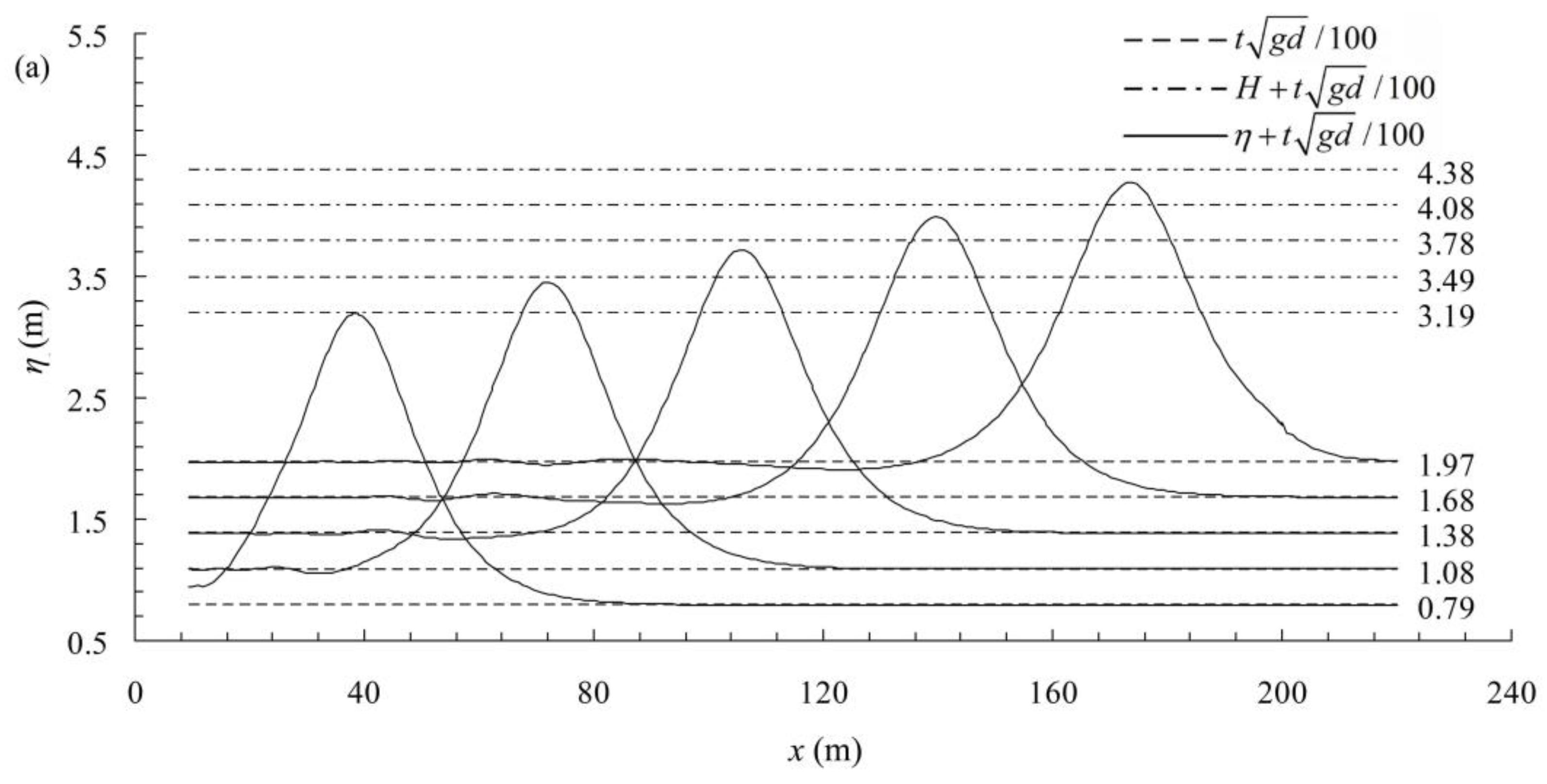

Figure 5.
Comparison between the numerical and analytical wave profile at t/τ = 1.1 for cases (a) #013, (b) #303, (c) #503, and (d) #103.
Figure 5.
Comparison between the numerical and analytical wave profile at t/τ = 1.1 for cases (a) #013, (b) #303, (c) #503, and (d) #103.

Figure 6.
Temporal evolution of the numerical free surface profile for case #103.

Figure 7.
Temporal evolution profiles at five sampling points for cases (a) #013 and (b) #103.

Figure 8.
Velocity magnitude contours at t/τ = 2.0 for cases (a) #013 (1 g) and (b) #103 (100 g).

Figure 9.
Velocity magnitude contours at t/τ = 3.0 for cases (a) #013 (1 g) and (b) #103 (100 g).
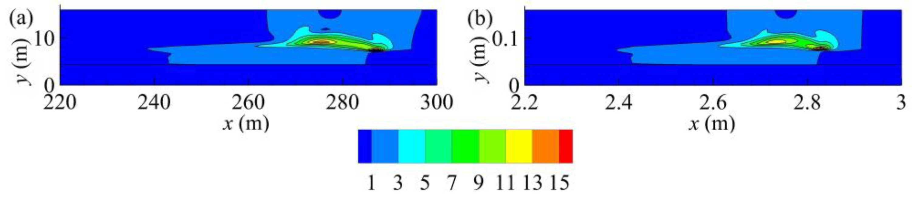
Figure 10.
The maximum dynamic pressure profiles for cases #013 and #103 at sampling point 2 (a) and sampling point 4 (b).
Figure 10.
The maximum dynamic pressure profiles for cases #013 and #103 at sampling point 2 (a) and sampling point 4 (b).


Table 1.
Summary of the basic centrifuge modeling scaling laws.
| Parameter | Dimension | Model Scaling (General) | Model Scaling (This Study) |
|---|---|---|---|
| Acceleration due to gravity | LT−2 | N | N |
| Wave length | L | n | 1/N |
| Wave height | L | n | 1/N |
| Water depth | L | n | 1/N |
| Piston stroke | L | n | 1/N |
| Time | T | N−1/2n1/2 | 1/N |
| Wave celerity | LT−1 | N1/2n1/2 | 1 |
| Density | ML−3 | 1 | 1 |
| Static pressure | ML−1T−2 | Nn | 1 |
| Kinematic viscosity coefficient | L2T−1 | N1/2n3/2 | 1 |
Table 2.
Overview of the experimental conditions performed in this study.
| Case Number | H (m) | d1 (m) | d2 (m) | H/d1 | d1/d2 | S (m) | τ (s) | L (m) | D (m) |
|---|---|---|---|---|---|---|---|---|---|
| Under the normal gravity (1 g) field | |||||||||
| 011 | 1.2 | 6 | 2.27 | 0.2 | 2.64 | 6.20 | 14.75 | 300 | 10 |
| 012 | 1.8 | 6 | 2.27 | 0.3 | 2.64 | 7.59 | 11.86 | ||
| 013 | 2.4 | 7 | 2.65 | 0.34 | 2.64 | 9.47 | 11.91 | 16 | |
| Under 30 times the normal gravity (30 g) field | |||||||||
| 301 | 0.04 | 0.2 | 0.076 | 0.2 | 2.64 | 0.21 | 0.49 | 10 | 0.33 |
| 302 | 0.06 | 0.2 | 0.076 | 0.3 | 2.64 | 0.25 | 0.40 | ||
| 303 | 0.08 | 0.23 | 0.088 | 0.34 | 2.64 | 0.32 | 0.40 | 0.53 | |
| Under 50 times the normal gravity (50 g) field | |||||||||
| 501 | 0.024 | 0.12 | 0.045 | 0.2 | 2.64 | 0.12 | 0.29 | 6 | 0.2 |
| 502 | 0.036 | 0.12 | 0.045 | 0.3 | 2.64 | 0.15 | 0.24 | ||
| 503 | 0.048 | 0.14 | 0.053 | 0.34 | 2.64 | 0.19 | 0.24 | 0.32 | |
| Under 100 times the normal gravity (100 g) field | |||||||||
| 101 | 0.012 | 0.06 | 0.023 | 0.2 | 2.64 | 0.06 | 0.15 | 3 | 0.1 |
| 102 | 0.018 | 0.06 | 0.023 | 0.3 | 2.64 | 0.08 | 0.12 | ||
| 103 | 0.024 | 0.07 | 0.027 | 0.34 | 2.64 | 0.09 | 0.12 | 0.16 | |
Table 3.
Numerical wave heights in the wave tank (units: cm).
| No. | 0.8 τ | 1.1 τ | 1.4 τ | 1.7 τ | 2.0 τ | εa (%) | No. | 0.8 τ | 1.1 τ | 1.4 τ | 1.7 τ | 2.0 τ | εa (%) |
|---|---|---|---|---|---|---|---|---|---|---|---|---|---|
| 011 | 121 | 120 | 119 | 118 | − | 0.19 | 501 | 2.39 | 2.34 | 2.31 | 2.28 | − | 0.40 |
| 012 | 181 | 179 | 177 | 175 | 174 | 0.30 | 502 | 3.53 | 3.43 | 3.37 | 3.32 | 3.28 | 0.62 |
| 013 | 240 | 237 | 234 | 231 | 230 | 0.34 | 503 | 4.66 | 4.51 | 4.41 | 4.34 | 4.30 | 0.71 |
| 301 | 3.98 | 3.91 | 3.85 | 3.81 | − | 0.36 | 101 | 1.19 | 1.17 | 1.15 | 1.14 | − | 0.36 |
| 302 | 5.89 | 5.72 | 5.61 | 5.53 | 5.47 | 0.64 | 102 | 1.77 | 1.72 | 1.68 | 1.66 | 1.64 | 0.65 |
| 303 | 7.76 | 7.52 | 7.36 | 7.24 | 7.16 | 0.69 | 103 | 2.33 | 2.26 | 2.21 | 2.17 | 2.14 | 0.69 |
© 2018 by the authors. Licensee MDPI, Basel, Switzerland. This article is an open access article distributed under the terms and conditions of the Creative Commons Attribution (CC BY) license (http://creativecommons.org/licenses/by/4.0/).
Share and Cite
MDPI and ACS Style
Wang, Q.-S.; Li, M.-H.; Li, D.-W. Solitary Wave Generation and Propagation under Hypergravity Fields. Water 2018, 10, 1381. https://doi.org/10.3390/w10101381
AMA Style
Wang Q-S, Li M-H, Li D-W. Solitary Wave Generation and Propagation under Hypergravity Fields. Water. 2018; 10(10):1381. https://doi.org/10.3390/w10101381
Chicago/Turabian StyleWang, Qiao-Sha, Ming-Hai Li, and Dai-Wei Li. 2018. "Solitary Wave Generation and Propagation under Hypergravity Fields" Water 10, no. 10: 1381. https://doi.org/10.3390/w10101381
Note that from the first issue of 2016, this journal uses article numbers instead of page numbers. See further details here.