Article

Flood Forecasting Based on an Improved Extreme Learning Machine Model Combined with the Backtracking Search Optimization Algorithm

1
School of Hydropower and Information Engineering, Huazhong University of Science and Technology, Wuhan 430074, China
2
Changjiang Institute of Survey, Planning, Design and Research, Wuhan 430010, China
3
Department of Geosciences, University of Oslo, 1047 Oslo, Norway
4
College of Resource and Environment, South-Central University for Nationalities, Wuhan 430074, China
*
Author to whom correspondence should be addressed.
Water 2018, 10(10), 1362; https://doi.org/10.3390/w10101362
Submission received: 6 September 2018 / Revised: 22 September 2018 / Accepted: 22 September 2018 / Published: 29 September 2018
(This article belongs to the Special Issue Flood Forecasting Using Machine Learning Methods)

Abstract

:
Flood forecasting plays an important role in flood control and water resources management. Recently, the data-driven models with a simpler model structure and lower data requirement attract much more attentions. An extreme learning machine (ELM) method, as a typical data-driven method, with the advantages of a faster learning process and stronger generalization ability, has been taken as an effective tool for flood forecasting. However, an ELM model may suffer from local minima in some cases because of its random generation of input weights and hidden layer biases, which results in uncertainties in the flood forecasting model. Therefore, we proposed an improved ELM model for short-term flood forecasting, in which an emerging dual population-based algorithm, named backtracking search algorithm (BSA), was applied to optimize the parameters of ELM. Thus, the proposed method is called ELM-BSA. The upper Yangtze River was selected as a case study. Several performance indexes were used to evaluate the efficiency of the proposed ELM-BSA model. Then the proposed model was compared with the currently used general regression neural network (GRNN) and ELM models. Results show that the ELM-BSA can always provide better results than the GRNN and ELM models in both the training and testing periods. All these results suggest that the proposed ELM-BSA model is a promising alternative technique for flood forecasting.

1. Introduction

Flood forecasting is not only an effective tool to reduce many risks posed by floods on life, property, and infrastructures, but can also provide valuable decision-making information for water resource managers [1,2,3,4]. However, due to streamflow affected by human activities and various hydro-meteorological factors, such as rainfall, topography, and surface heterogeneity, the runoff process exhibits highly non-linear, non-stationary, and complexly dynamic behaviors. Therefore, accurate flood forecasting, especially in the short-term (hourly or daily scale), has been recognized as a challenging work in hydrology.
Until now, plenty of hydrological models have been established to realize the flood forecasting [1]. These prediction models can be broadly classified into two kinds, namely physical-based models (also called knowledge-based models) and data-driven models (DDMs). The first group of models usually imitate the complex behaviors in the hydrologic cycle system by conceptualizing physical processes and basin characteristics, which often depends on detailed information and deep understanding about physical mechanisms of hydrological processes. Additionally, fine modelling of physical-based forecasting models using a full set of mathematic equations for each part in the hydrological cycle (i.e., interception, infiltration, evaporation) can theoretically reflect the real-world hydrological cycle more accurately, but this can lead to many intractable complications, such as the massive parameters to be estimated, the plenty of data requirements, and the expensive computational costs [5,6,7,8]. Compared with the physical-based models, the DDMs with a simpler model structure and less demanding data attract much more attention as an alternative forecasting tool in the cases that cannot reach the modelling conditions of physical-based models. Moreover, the rapid developments in computer sciences and some new technologies regarding machine learning, data mining, and optimization algorithms provide new opportunities for the DDMs in the application of various study domains including flood forecasting.
Over the last several decades, various DDMs were developed for flood forecasting, such as the artificial neural networks (ANNs) [1,9,10,11,12], adaptive neural-based fuzzy inference systems (ANFIS) [13,14], and support vector machines [15]. Among them, single hidden-layer feedforward neural networks (SLFNs), as the most widely used DDMs, show a strong ability to characterize any nonlinear mapping relationship, and have been taken as effective tools in solving many practical problems, such as flood forecasting [10,16,17,18], water level forecasting [19,20], and wind speed forecasting [21,22]. Although SLFNs have been successfully applied for modeling hydrological time series, they still suffer from several inherent disadvantages such as a slow learning process, easy plunging into local minima, and an over-fitting problem.
Recently, a novel learning algorithm for SLFN models, called the extreme learning machine (ELM), was developed by Huang et al. [23]. Compared with other typical SLFNs using gradient-based learning (GL) algorithms that learn parameters of a network in an iterative way, ELM is not involves less calculation work, higher learning speed, and stronger generalization ability, but also has no requirements for some parameters, such as terminating condition and learning rate. Considering these features, ELM has been applied as a promising non-linear fitting tool in massive complicated engineering applications [9,21,22]. For example, Yaseen et al. [24] applied the ELM for predicting the monthly streamflow discharge rates in a semi-arid region in Iraq and demonstrated its superiority over support vector regression (SVR) and general regression neural network (GRNN) models. In the same year, Deo and Şahin [20] testified the performance of ELM over conventional ANNs in forecasting mean streamflow water level based on many hydro-meteorological factors. More recently, Zhou et al. [9] developed a GRNN-based ensemble technique (GNE) for monthly streamflow forecasting, in which the results of three famous ANNs, namely radial basis function, ELM, and Elman networks, were fed into a GRNN model as the inputs.
Despite many successful applications of ELM in flood forecasting, it also results in an ill-conditioned problem in some cases because of its random mechanism in generating input weights and hidden layer biases. Therefore, it is necessary to introduce some effective techniques/tools to improve the generalization performance of the single ELM. To date, many endeavors have been made to enhance the stability of the basic ELM. The most famous way is that an evolutionary algorithm was adopted to search the optimal hidden node parameters of ELM. Han et al. [25] proposed a hybrid learning algorithm, in which an improved particle swarm optimization (IPSO) algorithm was applied to adjust the parameters of an ELM. Results showed that the developed IPSO-ELM approach had better generalization performance than the conventional ELM and the other evolutionary ELMs based on a differential evolution algorithm (DE) or PSO algorithm. Recently, a novel dual population-based iterative evolution algorithm, namely backtracking search optimization algorithm (BSA), was proposed in 2013 [26]. Since then, BSA has been used as an effective technique for searching global optimization. Unlike other widely used evolutionary algorithms (EAs), such as PSO, covariance matrix adaptation evolution strategy (CMAES), artificial bee colony algorithm (ABC), adaptive DE algorithm (JDE), comprehensive learning PSO (CLPSO), and self-adaptive DE algorithm (SADE), BSA has a simpler architecture with only one control parameter, and is insensitive to the initial value of its control parameter. All these features make BSA more effective, adaptive, and faster than other popular EAs. As such, BSA has already been applied to cope with many complex numerical optimization problems as an effective global searching algorithm [26]. However, until now, the capacity of BSA for dealing with the regression problems in the hydrological domain has never been explored.
Therefore, the major objective of this study is to develop a new, improved ELM (ELM-BSA) techniques for daily flood forecasting, which fuses the advantages of ELM and BSA. In the proposed ELM-BSA model, BSA was applied to find the suitable hidden node parameters of ELM, which can further promote the robustness of the standard ELM. The Yangtze River was selected as a case study. The measured daily streamflow data from the Yichang gauging station, the control site of the Three Gorges Reservoir (TGR), was employed to testify the performance of the proposed method. Moreover, two basic DDMs, namely ELM and GRNN models, which are recognized as the most efficient methods for flood forecasting [9,16,27], were selected as benchmark models for comparisons.
The paper is organized as follows. Section 2 introduces the proposed ELM-BSA method for short-term flood forecasting. Section 3 presents a case study of the upper Yangtze River and gives the forecasting results and comparisons with two basic data-driven models. All the conclusions of this study are summarized in Section 4.

2. Methodologies

2.1. Flood Forecasting Based on the Data-Diven Model

An analytic expression of a flood forecasting model can be defined as:
Q ( t ) = φ ( Q ( t d 1 + 1 ) , R ( t d 2 + 1 ) , E ( t d 3 + 1 ) )
where Q ( t ) is the predicted streamflow at time t; Q ( t d 1 + 1 ) represents the previous flow up to t d 1 + 1 time steps; R ( t d 2 + 1 ) stands for the antecedent rainfall with t d 2 + 1 time steps; E ( t d 3 + 1 ) is the other relevant factors up to t d 3 + 1 time steps that have main contributions to the flow at current time t, such as potential evapotranspiration, temperature, and/or the flow from major control stations in the upper reaches; di, I = 1, 2, 3 is the length of time lag for the relevant factors; and φ ( ) is a hydrological system transfer function to characterize the complicated nonlinear mapping relationship in a basin between flow and the relevant factors. Two kinds of methods can be used to estimate the φ ( ) . The first one is by using physical models (such as Xin’anjiang hydrological model). The second one is by using the data-driven models (i.e., ANN models).
Generally, flood forecasting based on data-driven models can be an alternative method for flood forecasting in some situations, such as when the observed data in the study area are inadequate and/or the potential physical mechanisms of hydrological phenomenon are unknown or only partially understood [8,28]. Moreover, DDMs are easy to establish and can provide acceptable forecasting results with less input data (only rainfall and/or flow data). Considering all these advantages of data-driven models, in this study we developed a new data-driven model named ELM-BSA for flood forecasting. In the new method, ELM, a novel data-driven model, was adopted as a base forecasting module to simulate the hydrological system transfer function φ ( ) . Meanwhile, BSA was applied to find the optimal input weights and biases of hidden layer nodes in the ELM to improve the stability of forecasting. The related methods and theories used in the new model, as well as its whole implementation, are presented as follows.

2.2. Extreme Learning Machine

An extreme learning machine (ELM) is an emerging fast-learning algorithm for SLFNs that usually has a three-layer structure with one input layer containing m nodes, one hidden layer containing h neurons, and a single output layer possessing p nodes (in flood forecasting, p is usually set to 1). Usually, the ELM model first randomly selects its input weights and hidden layer biases, and then analytically calculates its output weights using a least squares method instead of iterative adjusting. Therefore, ELM not only possesses the ability of an extremely fast learning speed, but also avoids frequent human intervention, which can provide better performance. These advantages make ELM more and more popular in handling many complex engineering problems.
For a given training sample set ( X j , t j ) with N pairs of observed data, where Xj is a multiple-dimensional input vector and tj is the target/desired output, the simulated output of ELM can be estimated using:
y j = i = 1 h β i g ( ω i X j + b i ) ,   j = 1 , 2 , , N
where y j is the output vector of the ELM model using the input vector Xj; β i denotes the weight vector connecting the ith hidden neuron to output layer neuron; g is the activation function for the hidden layer in ELM; ω i are the input weights connecting input layer neurons with the ith hidden layer neuron; and b i and g ( ω i X j + b i ) are the threshold and output of the ith hidden node, respectively.
The objective of an ELM is to search for a suitable set of β , ω , and b to approximate all training sample pairs with zero error:
j = 1 N t j y j = j = 1 N t j i = 1 h β i g ( ω i X j + b i ) = 0
Equation (3a) can be reorganized to be:
H β = T   where H = [ g ( ω 1 X 1 b 1 )   g ( ω 2 X 1 b 2 )   g ( ω h X 1 b h ) g ( ω 1 X 2 b 1 )   g ( ω 2 X 2 b 2 )   g ( ω h X 2 b h )                 g ( ω 1 X N b 1 )   g ( ω 2 X N b 2 )   g ( ω h X N b h ) ] N × h β = [ β 1   β 2     β h ] h × 1 1 ,   and   T = [ t 1   t 2     t N ] N × 1 1
where H is the output matrix of the hidden layer; β is the weights vector connecting the hidden layer nodes with the output layer neurons; and T represents the target output.
Once the random generation of the input hidden weights and biases of the hidden layer has been completed, ELM analytically calculates the hidden-output weights by searching a minimal norm least square solution of the following linear equation:
H β ^ T = min β H β T 0
The optimal estimated least squares solution of the above equation is:
β ^ = H T
where H denotes the Moore–Penrose generalized inverse of the hidden-layer output matrix H.

2.3. Backtracking Search Optimization Algorithm

Inspired by swarm behaviors, i.e., natural selection and information exchange between the populations, Civicioglu [26] proposed a novel population-based evolutionary algorithm called a backtracking search algorithm (BSA), which is a global searching technique to settle complex numerical optimization problems. In BSA, besides the famous operators used in the genetic algorithms (GAs) (i.e., the selection, mutation, and crossover operators), several particular mechanisms have also been employed, such as a memory system in which a population generated from a randomly selected historical generation is stored. Specifically, there are two populations in the BSA. One is the historical population and the other is the evolution population. In each iteration, the historical population is updated through random selection from both the historical population and the evolution population. Then, a new temporary population, called the trial population, is generated based on the mutation and crossover mechanisms. Finally, the trial population is used to update the evolution population based on a greedy selection mechanism. According to the research conducted by Civicioglu [26], the implementation of BSA consists of five major processes: initialization, selection-I, mutation, crossover, and selection-II. These five stages are simply summarized as follows:
(a) Initialization
In this phase, individuals of the historical population oldPop and evolution population Pop are randomly initialized within the predefined search space using a uniform distribution U as follows:
Pop i , j = U ( low j , up j ) , oldPop i , j = U ( low j , up j ) , i = 1 , 2 , , N pop ; j = 1 , 2 , , D
where N pop and D are the size of population and the dimension, respectively; and [ low j , up j ] are the preset upper and lower boundaries of the variables to be optimized.
(b) Selection-I
In this stage, an option is provided to update the oldPop at the start of each iteration according to the following “if-then” rule:
if   R 1 < R 2 then oldPop i , j = Pop i , j ,   R 1 , R 2 U ( 0 , 1 )
where R 1 and R 2 are two random numbers distributed uniformly from 0 to 1 to judge whether the historical population should be replaced by the evolution population in the current generation.
When oldPop is determined, the sequence of the individuals in oldPop is then changed by a random shuffling function permuting ( ) :
oldPop : = permuting ( oldPop )
where “ := ” indicates the update operator.
(c) Mutation
In this step, the temporary population, called trial population trialPop, is initialized using
trialPop = Pop + F ( oldPop Pop ) F = 3 rndn ,   rndn ~ N ( 0 , 1 )
where ( oldPop Pop ) denotes the search direction matrix whose amplitude can be controlled by a control parameter F.
Due to the utilization of oldPop in the mutation operation, BSA can learn partial experiences from previous generations.
(d) Crossover
The final form of the trial population is determined in this stage. The crossover operator starts with a generation of a binary integer-valued matrix ( map N pop × D ) to determine which elements of population have to be manipulated. The crossover operator is realized using
trialPop i j = { Pop ij ,   if   map ij = 1 trialPo p ij , otherwise
(e) Selection-II
In this phase, the population of the next generation is generated according to a greedy selection strategy. The trial individuals with better fitness values are used to update the corresponding individuals in population Pop ij :
Pop ij = { trialPop ij , if fitness ( trialPop ij ) < fitness ( Pop ij ) Pop ij ,              otherwise

2.4. The Proposed ELM-BSA Model for Flood Forecasting

As discussed in the introduction, ELM can save the calculation time by randomly generating network parameters instead of arduously tuning them. Compared with the traditional SLFNs with GL algorithms, ELM not only has a faster training speed and better generalization capability but also avoids the predefining computational parameters including the learning rate and stopping criteria. These advantages of ELM make it more suitable for solving the complex non-linear optimization problem, i.e., flood forecasting. Unfortunately, the random generation of input weights and hidden layer thresholds in ELM may provide some non-optimal or unnecessary network parameters which may reduce the prediction reliability, increase uncertainty of forecasting results, and produce unacceptable results for practical applications. To settle this problem, we proposed an ELM-BSA model, in which the input weights and thresholds of hidden layer neurons were optimized using BSA in the training period.
The construction of the ELM-BSA for flood forecasting is set to m-h-1 due to there being only one node in the output layer. The implementation of the proposed model is described as follows:
Step 1: Normalize the original time series into the range [0, 1] using Equation (12), and then partition the normalized series into two parts: training and testing datasets.
Q i nor = Q i Q min Q max Q min
where Q i nor and Q i are the normalized and observed streamflow, respectively; and Q min and Q max represent the minimum and maximum values of the original data, respectively.
Step 2: Initialize the related parameters of the proposed ELM-BSA model, such as the population size Npop and the maximum iteration K.
Step 3: Define the architecture of the ELM and its activation function of hidden neurons, which is set to the sigmoid function in this study.
Step 4: Set the initial iteration number k = 1, and then initialize the historical population oldPop and evolution population Pop according to Equation (6). Each individual contains all parameters of the hidden layer, hence the ith individual in the kth generation can be written as
para ( i , k ) = [ ω 1 , ( i , k ) T , ω 2 , ( i , k ) T , , ω h , ( i , k ) T , b 1 , ( i , k ) , b 2 , ( i , k ) , , b h , ( i , k ) ]
where ω 1 , ( i , k ) T , ω 2 , ( i , k ) T , , ω h , ( i , k ) T represent the weight vector that connect the input nodes with the hidden layer neurons; and b 1 , ( i , k ) , b 2 , ( i , k ) , , b h , ( i , k ) are the thresholds for the hidden layer neurons.
Step 5: Calculate the output weights and initialize fitness values of all individuals of the population Pop using Equations (14) and (15), respectively.
         β ^ ( i , k ) = H ( i , k ) T H ( i , k ) = [ g ( ω 1 , ( i , k ) X 1 + b 1 , ( i , k ) )   g ( ω 2 , ( i , k ) X 1 + b 2 )   g ( ω h , ( i , k ) X 1 + b h , ( i , k ) ) g ( ω 1 , ( i , k ) X 2 + b 1 , ( i , k ) )   g ( ω 2 , ( i , k ) X 2 + b 2 )   g ( ω h , ( i , k ) X 2 + b h , ( i , k ) )                   g ( ω 1 , ( i , k ) X N + b 1 , ( i , k ) )   g ( ω 2 , ( i , k ) X N + b 2 )   g ( ω h , ( i , k ) X N + b h , ( i , k ) ) ] N × h
f [ para ( i , k ) ] = 1 N j = 1 N ( t j y j ) 2 = 1 N j = 1 N ( t j i = 1 h β i g ( ω i X j + b i ) ) 2
where H ( i , k ) is Moore–Penrose generalized inverse of the hidden-layer output matrix H ( i , k ) for the ith individual in the kth generation; y j and t j are the calculated and target output in the training stage, respectively; and N is the total number of the training samples.
Step 6: Generate the historical population OldPop using the selection-I operator and obtain the initial form of the trial population trialPop using mutation operator.
Step 7: Apply the mutation operator on both the historical population and the trial population trialPop to generate the final form of the trial population.
Step 8: Calculate the fitness values of all individuals at the current generation, and then update individuals of the next generation through selection-II strategy.
Step 9: Set k = k + 1. If the maximum iteration is reached, go to Step 10; otherwise, go to Step 6.
Step 10: Apply the well-tuned ELM model to the forecasting phase using the validated dataset. Note, the output values of the forecasting model should be de-normalized to the range of the target output dataset.

2.5. Performance Indexes

Several indexes including coefficient of correlation (r), Nash–Sutcliffe coefficient of efficiency (NSE), root mean square error (RMSE), and mean absolute error (MAE) were employed to evaluate the performance of the proposed model. Equations for these indexes are given as follows.
r = ( i = 1 N ( Q obs , i Q ¯ obs ) ( Q fore , i Q ¯ fore ) i = 1 N ( Q o b s , i Q ¯ o b s ) 2 i = 1 N ( Q f o r e , i Q ¯ fore ) 2 ) , 1 < r < 1
NSE = 1 ( i = 1 N ( Q o b s , i Q f o r e , i ) 2 i = 1 N ( Q o b s , i Q ¯ o b s ) 2 ) , NSE 1
RMSE = 1 N i = 1 N ( Q o b s , i Q f o r e , i ) 2 , RMSE > 0
MAE = 1 N i = 1 N | Q o b s , i Q f o r e , i | , MAE > 0
where Q o b s , i and Q f o r e , i are the ith observed and predicted values of runoff, respectively; Q ¯ obs and Q ¯ fore are the average values of the observed and forecasted runoff, respectively; and N is the length of the data set.
Moreover, the Chinese flood forecasting standard recommend the use of the qualified rate (QR) to evaluate the flood forecasting performances [29]. A predicted peak value is regarded as “qualified” when the relative absolute error (RAE) between the predicted and the measured streamflow value is within the given threshold value [30]. The QR can be calculated using
QR = i = 1 N num i N × 100 %    where num i = { 1 , i f ( RAE i ε ) 0 ,    otherwise , RAE i = | Q o b s , i Q f o r e , i | Q o b s , i
where RAE i is the relative absolute error (RAE) of the ith datum; num i is set to 1 when RAE is less than or equal to the predefined threshold value ( ε ), which is regarded as qualified forecasting. The ε is set to 20% in accordance with the Chinese forecasting standard (GB/T 22482-2008) [31].

3. Case Study

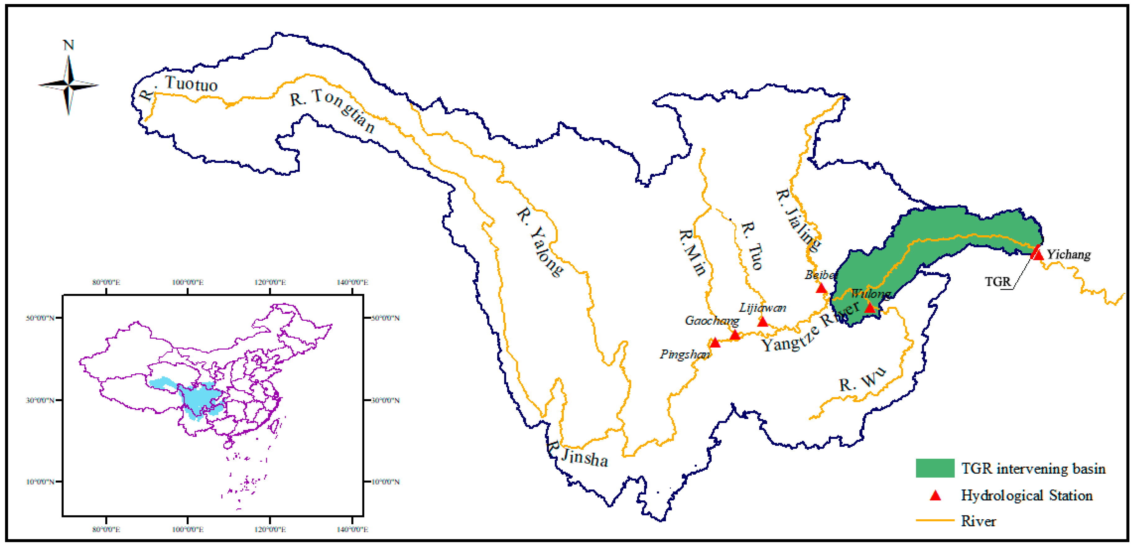
3.1. Study Area and Data

To validate the efficacy of the proposed model, the Yangtze River, which is the longest river in Asia and the third longest river in the world, was selected as a case study because abundant and detailed historical daily runoff data have been collected. The Yangtze River, which is nearly 6300 km long, originates from east of the Tibetan Plateau and flows eastward to the East China Sea in Shanghai city [10].
This study mainly focused on the upper Yangtze River, which covers a total area of nearly 1 million km2, accounting for about 56% of the whole area of the Yangtze River, with a total length of 4529 km, up to 75% of the entire length of the Yangtze River. Flood events frequently occur in this region. During the historical years, extreme flood events, especially for the years 1870, 1954, 1998, 2010, and 2016, have caused heavy casualties and property losses. For example, in 2016, the whole Yangtze River basin suffered from a monstrous flood, which led to economic losses of 146.9 billion Chinese Yuan and affected nearly 60.74 million people [32,33]. Accordingly, flood forecasting is an essential task for modern flood prevention and disaster relief of the upper Yangtze River.
Floods in the Yangtze River usually occur in monsoon season between June and September. During this period, the temporal and spatial distribution characteristics of regional rainfall depend heavily on monsoon activities and seasonal movement of subtropical anticyclones. Floods in the middle-lower Yangtze River mainly come from the upper region of the Yichang Station, a control hydrological station of the Three Georges Reservoir (TGR) which is situated at an intersection point of the upstream Yangtze River and the middle reaches [34,35]. The main tributaries in the upper Yangtze River from upstream to downstream are Yalong, Min, Tuo, Jialing, and Wu Rivers as shown in Figure 1, where the control stations of each tributary are also given. In this study, the Jinsha River, rather than the Yalong River, was taken into account, because the Yalong River flows into the Jinsha River, which is considered part of the Yangtze River [10]. As shown in Figure 1, six gauging stations named Pingshan, Gaochang, Lijiawan, Beibei, Wulong, and Yichang located in these rivers were considered. Each of them has a concurrent mean daily flow data from the year 1998 to year 2007. The historical streamflow of Yichang Station and its upstream stations were taken as alternative input factors, and the streamflow of Yichang station at time t was considered as output. In other words, the proposed forecasting model aims to predict the outflow of the TGR. The data set was divided into subsets, in which the daily streamflow data from the year 1998 to 2005 was employed for model calibration, and the data from the year 2006 to 2007 for model validation.

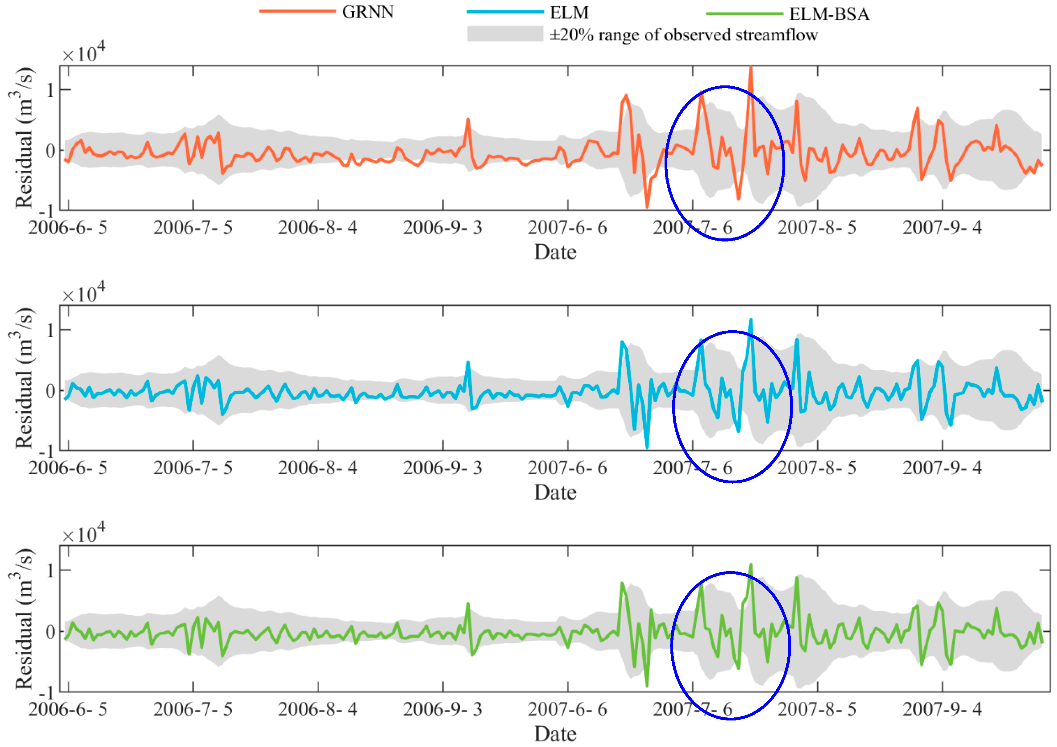
3.2. Establishment of the Flood Forecasting Models

Determination of model inputs is the most significant step for the data-driven forecasting model. The data-driven approaches may provide unreliable results when the inputs contain irrelevant or redundant information. However, there is no uniform approach to determine the input variables. According to a review conducted by Bowden et al. [11], the major approaches for input determination/selection in hydrological forecasting can be divided into three groups: trial and error method, linear method, and non-linear method. Considering the demerits and merits of these methods, a linear method called partial cross-correlation (PCC) [11] and a nonlinear approach called entropy based-partial mutual information (PMI) proposed by Chen et al. [10] were selected and compared. In the entropy based-PMI method, entropy theory, a famous tool to derive distribution functions [36,37], was combined with copula functions to predigest the solving process of PMI. Therefore, using these three techniques, seven different input combination schemes were obtained as shown in Table 1, where φ ( ) indicates the complicated nonlinear mapping function between the input factors and the output results and Q p s , Q g c , Q l j w , Q b b , Q w l , and Q y c indicate the streamflow of the Pingshan, Gaochang, Lijiawan, Beibei, Wulong, and Yichang gauging stations, respectively, and t represents the current time.
The input sets of the first five schemes M1 to M5 were designed according to the trial and error method, and schemes M6 and M7 were determined by Chen et al. [10] based on the PCC and PMI approaches, respectively. It can be seen that the first five schemes M1 to M5 only considered the historical runoff of the Yichang station ( Q y c ), whereas schemes M6 and M7 used both the anterior runoff from the Yichang station and those from all control stations of the main tributaries located on the upper Yangtze River as input variables. All of the seven input sets were fed into ELM-BSA, GRNN, and ELM models to train.
In addition, the number of hidden neurons also plays an important role for establishment of the forecasting models. To obtain the suitable number of hidden neurons, a grid search algorithm was employed in this study. For the proposed ELM-BSA model, the parameters of the BSA were set to Npop = 30 and K = 100. All forecasting models established in this study were encoded based on the Matrix Laboratory (MATLAB R2015a) platform manufactured by Mathwork Incoperation, Springfield, MA, USA.

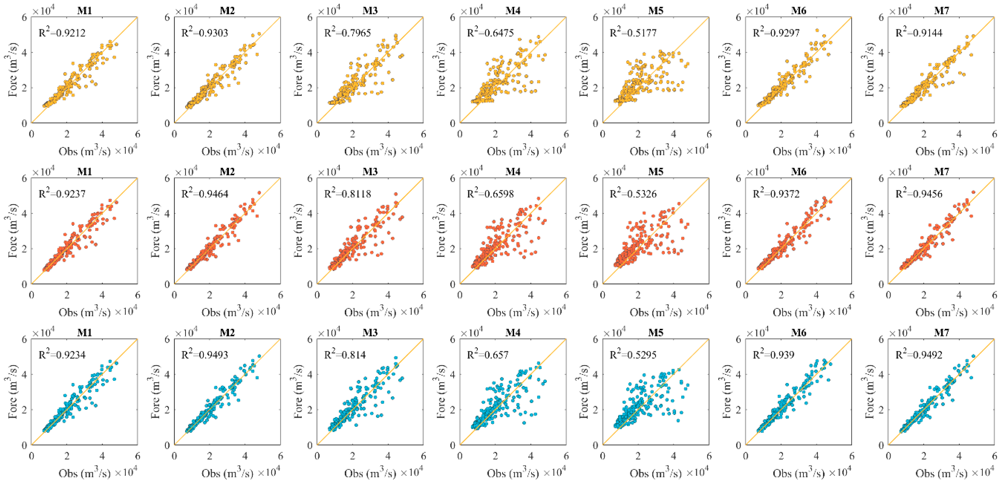
3.3. Sensitivity Analysis of Different Input Sets

To testify the efficiency of the proposed ELM-BSA model, the GRNN and ELM models were selected as benchmark models. Input selection is one of the important steps for flood forecasting based on the data-driven method. Hence, all seven input schemes mentioned in Table 1 were taken into account in this study. The GRNN, ELM, and the proposed ELM-BSA models were employed for flood forecasting of the Yichang station located on the Yangtze River. Five performance indexes were used to evaluate the efficiency of the above three forecasting models. The data set was divided into two sub-sets. The first 8 years (from the year 1998 to year 2005) was used for model calibration and the remaining 2 years (from the year 2006 to year 2007) were used for model validation. Results of the three models for both the training and testing periods are given in Table 2, where the model with the best performance is highlighted in bold. It can be seen that compared with the GRNN and ELM models, the proposed ELM-BSA model performed better based on the values of the three indexes, no matter what the input combinations were. The most appropriate model inputs were not the same for the three forecasting models and the response of each forecasting model was not identical when using the same input sets. In other words, accurate forecasting results were not only affected by the inputs, but also by the model structure and its corresponding parameters. This also indicates that obtaining the accurate flood forecasting results is a complicated and challenging task under the comprehensive effects of model inputs, structures, and parameters.
It can be seen from Table 2 that when the GRNN model was used, the model with the M2 input set produced the best forecasting results in both the training and validation periods. Similarly, the ELM based on the M2 yielded the best forecasting results for both the training and testing periods. For the proposed ELM-BSA method, it demonstrated that the model with the M7 input sets showed better performances. Overall, the most suitable input sets for the GRNN, ELM, and ELM-BSA models were M2, M2, and M7 respectively.
To further compare the predicted streamflow with the observed flow, the predicted and observed flow were drawn in the same figure as shown in Figure 2, where the x-axis represents the observed flow and the y-axis represents the predicted flow. If the model works well, the predicted flow should be equal to the observed flow. Results of the three flood forecasting models with seven input schemes M1–M7 in the validation period are shown in Figure 2. The regression coefficient R2 was also calculated and displayed in Figure 2. If the predicted and observed streamflow being compared are similar, the scatter points should approximately lie on the line y = x, namely the diagonal line shown in Figure 2. It can be seen that according to the R2 and fitting results, the input schemes M1, M2, M6, and M7 for both of the three models could always provide better results than other input schemes. For the forecasting models based on the input set selected by the PMI method, M7 provided slightly better results than those based on the inputs chosen by the PCC approach, namely M6. It can also be seen from Table 2 and Figure 2 that the three models with input schemes M1 and M2 showed better performances than those models with the schemes M3 to M5. This means that when more anterior flows, such as the flows at lag time t-3, t-4, and t-5, are considered, the performance of the models became worse, which means more inputs bring noise to the forecasting system. Meanwhile, models based on different input sets yielded different results, while the best input sets were not identical for all forecasting models. According to the results of Figure 2 and Table 2, the best input combinations for the GRNN, ELM, and ELM-BSA models were M2, M2, and M7, respectively. Figure 2 also demonstrates that the proposed ELM-BSA model with the M7 input set performed best among all the combinations of inputs and models with the R2 value of 0.9492.
Table 3 summarizes the best performance results calculated using the three models with different input sets. It indicates that compared with other methods, there were significant improvements when the ELM-BSA was used. The ELM-BSA model provided better forecasting results than the GRNN and ELM models for daily streamflow forecasting. For the validation period, compared with the GRNN model, when the ELM-BSA model was used, the performance indexes r, NSE, RMSE, and QR increased by 1.05%, 3.12%, and 13.64%, respectively, and the indexes RMSE and MAE decreased by 19.63% and 27.22%, respectively. Similarly, compared with the standard ELM model, when the ELM-BSA was used, the indexes r, NSE, RMSE, and QR increased by 0.15%, 0.4%, and 1.32%, respectively, and the indexes RMSE and MAE decreased by 3.42% and 4.72%, respectively. Therefore, the proposed method increased the flood forecasting model accuracy.
As streamflow in the flood season has a great impact on the scientific decision-making of modern water resources management and planning, the number of forecasting values whose relative error beyond the specific range (±15%, ±20%, and ±25%) are given in Table 4, where the number and proportion of over-ranging points for each forecasting model in the testing period are shown. Results indicate that the total number of over-ranging points of the ELM-BSA model was always less than the other two models for each specific range. This means that the ELM-BSA model performed better than GRNN and ELM for the daily streamflow forecasting. The advantages of the ELM-BSA model for high streamflow forecasting can be visually seen in Figure 3, where the residual values of the best ELM-BSA, GRNN, and ELM models in the validation period are presented, and the ±20% intervals of the observed streamflow is also presented. Results show that the ELM-BSA produced the best performance because it provided fewer residual values falling outside the ±20% range than the other two models. For example, its residual value out of the reference range between the date 6 July 2007, and 5 August 2007 (marked in Figure 3) was comparatively less serious. Meanwhile, the ELM-BSA model produced smaller maximum residual values than the other two models, while the GRNN performed even worse than the ELM. Additionally, the GRNN model was not suitable for the low and high streamflow parts due to its remarkable over-estimation and under-estimation. All these results imply that the proposed model was superior to the other models for flood forecasting.

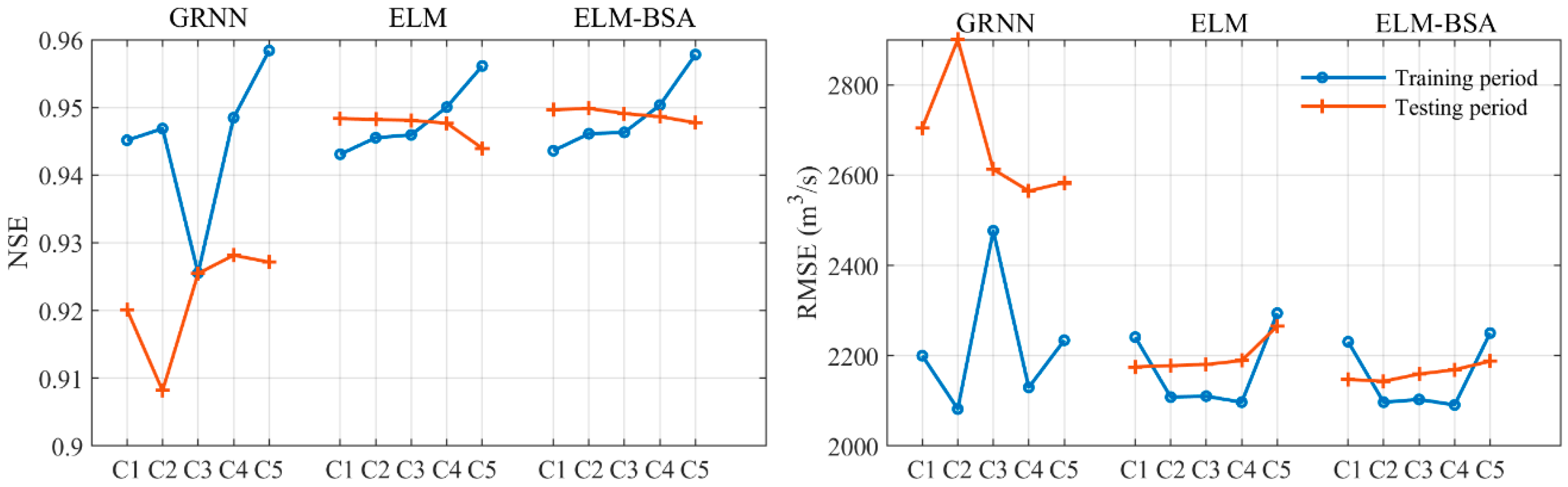
3.4. Sensitivity Analysis of Different Training Sample Sizes

Another important factor affecting the forecasting accuracy of data-driven forecasting models is the number of training samples. Hence, in this sub-section, five schemes were designed and employed to further test the performances of the proposed ELM-BSA model with different training data sizes. In each case, the same dataset, the data from the last two years (from the year 2006 to year 2007), was used for model validation. Performances of the ELM-BSA model in these five scenarios are given in Table 5. Meanwhile, Figure 4 shows the values of indexes RMSE and NSE calculated using ELM-BSA with different training data sizes. ELM-BSA with a different number of training data demonstrate different forecasting results and all these results can comply with the Chinese flood forecasting standard [31]. Hence, these models developed in this study can be applied to practical use. Meanwhile, the forecasting accuracies of the ELM-BSA model were always better than the other two models in all cases, because the ELM-BSA model could yield the largest NSE values and the lowest RMSE values in the validation period among these three forecasting models. In the training period, the forecasting accuracies grew with the increase of training data size, except for the GRNN model with Case 3. In the validation period, the ELM and ELM-BSA models provided stable NSE values for Cases 1–4, while there is a sudden drop of NSE in Case 5 for ELM. The forecasting accuracies of GRNN in the validation period increased with the increase of the training samples, except for Case 2. The ELM and ELM-BSA could generate stable RMSE values for Cases 2–4 in the training period and for Cases 1–4 in the testing period. As for GRNN, its performances in the testing stage seemed to be better when the training samples were increased, whereas its performance fluctuated in the training period with an increase of the training samples. Additionally, Figure 4 clearly shows that the training number in the Case 3 was the best one for all the forecasting models, because in this condition, the accuracies in both training and testing periods for every forecasting model were well-balanced. These results indicate that more samples adopted to train forecasting model may be conductive to enhancing the forecasting accuracy of the training stage but may be detrimental to the performance in the testing phase in the condition where the number of training samples exceeds a specific range. Therefore, in the real engineering applications, it is important to balance the sample sizes of the training and testing datasets, which will be helpful to promote the robustness and accuracy of the forecasting models. All the above results prove the superiority of the ELM-BSA model in the aspects of both robustness and accuracy when compared with the other two widely used forecasting models. This is due to the fact that the ELM-BSA model processes the merits of both the BSA and ELM, which enhances its generalization ability and robustness.
In summary, all the above results obtained from Section 3.3 and Section 3.4 indicate that the ELM-BSA model is a powerful tool to model the daily streamflow and can produce more reliable performance compared with GRNN and ELM. It provides an effective alternative for flood forecasting.

4. Conclusions

Reliable and robust flood forecasting plays an essential role in effective/scientific flood control and many activities associated with water resources management. On the basis of an extreme learning machine (ELM) and an emerging dual population-based evolutionary algorithm named backtracking search optimization algorithm (BSA), this paper developed an improved extreme learning machine named ELM-BSA for short-term flood forecasting. In the new forecasting model, BSA was used to find the appropriate hidden node parameters of ELM, and then the well-tuned ELM was applied to do one-step-ahead forecasting. For the purpose of evaluating the performance of the developed model, the standard ELM and a widely-used GRNN model were taken as reference models. The upper Yangtze River was selected as a case study. Experiments with different input combination schemes and training sample sizes indicated that the proposed ELM-BSA model was superior to the current ELM and GRNN models. For example, compared with the GRNN model, the improvements achieved by the ELM-BSA model regarding the indexes NSE and RMSE values in the validation period were 3.12% and 19.63%, respectively. Moreover, when the sample size changed within a proper range, the accuracy of the developed model fluctuated in a smaller scope than those of the ELM and GRNN models, which demonstrated the stability of the proposed model. Therefore, the ELM-BSA model is a powerful tool for flood forecasting. It is necessary to apply this new method to real-time flood forecasting.

Author Contributions

L.C. designed this experiment and write parts of the paper; N.S. and Q.Z. did the calculation work and wrote parts of the paper. C.Z., J.Z. (Jianzhong Zhou), Y.Z., J.Z. (Junhong Zhang) made some corrections to the paper.

Funding

This research was funded by the National Key R & D Program of China (2017YFC0405900) and the National Natural Science Foundation of China (91547208; 51879109).

Acknowledgments

The authors also greatly appreciate the anonymous reviewers and academic editor for their careful comments and valuable suggestions to improve the manuscript.

Conflicts of Interest

The authors declare no conflict of interest.

References

  1. Yaseen, Z.M.; El-Shafie, A.; Jaafar, O.; Afan, H.A.; Sayl, K.N. Artificial intelligence based models for stream-flow forecasting: 2000–2015. J. Hydrol. 2015, 530, 829–844. [Google Scholar] [CrossRef]
  2. Chen, L.; Singh, V.P.; Guo, S. Measure of correlation between river flows using the copula-entropy method. J. Hydrol. Eng. 2013, 18, 1591–1606. [Google Scholar] [CrossRef]
  3. Chen, L.; Singh, V.P.; Lu, W.; Zhang, J.; Zhou, J.; Guo, S. Streamflow forecast uncertainty evolution and its effect on real-time reservoir operation. J. Hydrol. 2016, 540, 712–726. [Google Scholar] [CrossRef]
  4. Huang, K.; Ye, L.; Chen, L.; Wang, Q.; Dai, L.; Zhou, J.; Singh, V.P.; Huang, M.; Zhang, J. Risk analysis of flood control reservoir operation considering multiple uncertainties. J. Hydrol. 2018, 565, 672–684. [Google Scholar] [CrossRef]
  5. Costabile, P.; Costanzo, C.; Macchione, F. A storm event watershed model for surface runoff based on 2D fully dynamic wave equations. Hydrol. Process. 2013, 27, 554–569. [Google Scholar] [CrossRef]
  6. Rousseau, M.; Cerdan, O.; Delestre, O.; Dupros, F.; James, F.; Cordier, S. Overland flow modeling with the shallow water equations using a well-balanced numerical scheme: Better predictions or just more complexity. J. Hydrol. Eng. 2015, 20, 04015012. [Google Scholar] [CrossRef]
  7. Bout, B.; Jetten, V.G. The validity of flow approximations when simulating catchment-integrated flash floods. J. Hydrol. 2018, 556, 674–688. [Google Scholar] [CrossRef]
  8. Bellos, V.; Tsakiris, G. A hybrid method for flood simulation in small catchments combining hydrodynamic and hydrological techniques. J. Hydrol. 2016, 540, 331–339. [Google Scholar] [CrossRef]
  9. Zhou, J.; Peng, T.; Zhang, C.; Sun, N. Data pre-analysis and ensemble of various artificial neural networks for monthly streamflow forecasting. Water 2018, 10, 628. [Google Scholar] [CrossRef]
  10. Chen, L.; Ye, L.; Singh, V.; Asce, F.; Zhou, J.; Guo, S. Determination of input for artificial neural networks for flood forecasting using the copula entropy method. J. Hydrol. Eng. 2014, 19, 217–226. [Google Scholar] [CrossRef]
  11. Bowden, G.J.; Dandy, G.C.; Maier, H.R. Input determination for neural network models in water resources applications. Part 1—Background and methodology. J. Hydrol. 2005, 301, 75–92. [Google Scholar] [CrossRef]
  12. Chang, F.-J.; Tsai, M.-J. A nonlinear spatio-temporal lumping of radar rainfall for modeling multi-step-ahead inflow forecasts by data-driven techniques. J. Hydrol. 2016, 535, 256–269. [Google Scholar] [CrossRef]
  13. Chang, F.J.; Lai, H.C. Adaptive neuro-fuzzy inference system for the prediction of monthly shoreline changes in northeastern taiwan. Ocean Eng. 2014, 84, 145–156. [Google Scholar] [CrossRef]
  14. Zhou, Y.; Chang, F.J.; Guo, S.; Ba, H.; He, S. A robust recurrent anfis for modeling multi-step-ahead flood forecast of three gorges reservoir in the yangtze river. Hydrol. Earth Syst. Sci. Discuss. 2017, 1–29. [Google Scholar] [CrossRef]
  15. Xing, B.; Gan, R.; Liu, G.; Liu, Z.; Zhang, J.; Ren, Y. Monthly mean streamflow prediction based on bat algorithm-support vector machine. J. Hydrol. Eng. 2016, 21, 04015057. [Google Scholar] [CrossRef]
  16. Tayyab, M.; Zhou, J.; Dong, X.; Ahmad, I.; Sun, N. Rainfall-runoff modeling at jinsha river basin by integrated neural network with discrete wavelet transform. Meteorol. Atmos. Phys. 2017, 129, 1–11. [Google Scholar] [CrossRef]
  17. Peng, T.; Zhou, J.; Zhang, C.; Fu, W. Streamflow forecasting using empirical wavelet transform and artificial neural networks. Water 2017, 9, 406. [Google Scholar] [CrossRef]
  18. Cheng, C.; Niu, W.; Feng, Z.; Shen, J.; Chau, K. Daily reservoir runoff forecasting method using artificial neural network based on quantum-behaved particle swarm optimization. Water 2015, 7, 4232–4246. [Google Scholar] [CrossRef]
  19. Chang, F.J.; Chen, P.A.; Lu, Y.R.; Huang, E.; Chang, K.Y. Real-time multi-step-ahead water level forecasting by recurrent neural networks for urban flood control. J. Hydrol. 2014, 517, 836–846. [Google Scholar] [CrossRef]
  20. Deo, R.C.; Şahin, M. An extreme learning machine model for the simulation of monthly mean streamflow water level in eastern queensland. Environ. Monit. Assess. 2016, 188, 90. [Google Scholar] [CrossRef] [PubMed]
  21. Zhou, J.; Sun, N.; Jia, B.; Tian, P. A novel decomposition-optimization model for short-term wind speed forecasting. Energies 2018, 11, 1572. [Google Scholar] [CrossRef]
  22. Li, C.; Xiao, Z.; Xia, X.; Zou, W.; Zhang, C. A hybrid model based on synchronous optimisation for multi-step short-term wind speed forecasting. Appl. Energy 2018, 215, 131–144. [Google Scholar] [CrossRef]
  23. Huang, G.; Zhu, Q.; Siew, C. Extreme learning machine: Theory and applications. Neurocomputing 2006, 70, 489–501. [Google Scholar] [CrossRef] [Green Version]
  24. Yaseen, Z.M.; Jaafar, O.; Deo, R.C.; Kisi, O.; Adamowski, J.; Quilty, J.; El-Shafie, A. Stream-flow forecasting using extreme learning machines: A case study in a semi-arid region in iraq. J. Hydrol. 2016, 542, 603–614. [Google Scholar] [CrossRef]
  25. Han, F.; Yao, H.F.; Ling, Q.H. An improved evolutionary extreme learning machine based on particle swarm optimization. Neurocomputing 2013, 116, 87–93. [Google Scholar] [CrossRef]
  26. Civicioglu, P. Backtracking search optimization algorithm for numerical optimization problems. Appl. Math. Comput. 2013, 219, 8121–8144. [Google Scholar] [CrossRef]
  27. Chen, L.; Singh, V.P.; Guo, S.; Zhou, J.; Ye, L. Copula entropy coupled with artificial neural network for rainfall–runoff simulation. Stoch. Environ. Res. Risk Assess. 2014, 28, 1755–1767. [Google Scholar] [CrossRef]
  28. Hosseini, S.M.; Mahjouri, N. Integrating support vector regression and a geomorphologic artificial neural network for daily rainfall-runoff modeling. Appl. Soft Comput. 2016, 38, 329–345. [Google Scholar] [CrossRef]
  29. Chen, L.; Zhang, Y.; Zhou, J.; Singh, V.P.; Guo, S.; Zhang, J. Real-time error correction method combined with combination flood forecasting technique for improving the accuracy of flood forecasting. J. Hydrol. 2014, 521, 157–169. [Google Scholar] [CrossRef]
  30. Li, X.; Guo, S.; Liu, P.; Chen, G. Dynamic control of flood limited water level for reservoir operation by considering inflow uncertainty. J. Hydrol. 2010, 391, 126–134. [Google Scholar] [CrossRef]
  31. Ministry of Water Resources (MWR). Regulation for Calculating Design Flood of Water Resources and Hydropower Projects; Chinese Shuili Shuidian Press: Beijing, China, 2008. (In Chinese) [Google Scholar]
  32. Huang, K.D.; Chen, L.; Zhou, J.; Zhang, J.; Singh, V.P. Flood hydrograph coincidence analysis for mainstream and its tributaries. J. Hydrol. 2018, 565, 341–353. [Google Scholar] [CrossRef]
  33. Zhou, C.; Sun, N.; Chen, L.; Ding, Y.; Zhou, J.; Zha, G.; Luo, G.; Dai, L.; Yang, X. Optimal operation of cascade reservoirs for flood control of multiple areas downstream: A case study in the upper Yangtze river basin. Water 2018, 10, 1250. [Google Scholar] [CrossRef]
  34. Chen, L.; Singh, V.P.; Guo, S.L.; Hao, Z.C.; Li, T.Y. Flood coincidence risk analysis using multivariate copula functions. J. Hydrol. Eng. 2012, 17, 742–755. [Google Scholar] [CrossRef]
  35. Chen, L.; Singh, V.P.; Guo, S.; Zhou, J.; Zhang, J. Copula-based method for multisite monthly and daily streamflow simulation. J. Hydrol. 2015, 528, 369–384. [Google Scholar] [CrossRef]
  36. Chen, L.; Singh, V.; Huang, K. Bayesian technique for the selection of probability distributions for frequency analyses of hydrometeorological extremes. Entropy 2018, 20, 117. [Google Scholar] [CrossRef]
  37. Chen, L.; Singh, V.P. Entropy-based derivation of generalized distributions for hydrometeorological frequency analysis. J. Hydrol. 2018, 557, 699–712. [Google Scholar] [CrossRef]
Figure 1. Locations of hydrological stations in the study area.
Water 10 01362 g001
Figure 2. Scatter plots of observed (Obs) and predicted (Fore) runoff provided by the GRNN (the first row), ELM (the second row), and ELM-BSA (the third row) models with different input sets.
Water 10 01362 g002
Figure 3. Residual values of the three models in the validation period.
Water 10 01362 g003
Figure 4. NSE and RMSE values of ELM-BSA, GRNN, and ELM in five cases with different training sample sizes.
Water 10 01362 g004
Table 1. Different input sets calculated by trial and error, PCC and PMI approaches.
SchemesNumber of Input Variables Established Models
M11 Q y c ( t ) = φ [ Q y c ( t 1 ) ]
M22 Q y c ( t ) = φ [ Q y c ( t 1 ) , Q y c ( t 2 ) ]
M33 Q y c ( t ) = φ [ Q y c ( t 1 ) , Q y c ( t 2 ) , Q y c ( t 3 ) ]
M44 Q y c ( t ) = φ [ Q y c ( t 1 ) , Q y c ( t 2 ) , Q y c ( t 3 ) , Q y c ( t 4 ) ]
M55 Q y c ( t ) = φ [ Q y c ( t 1 ) , Q y c ( t 2 ) , Q y c ( t 3 ) , Q y c ( t 4 ) , Q y c ( t 5 ) ]
M66 Q y c ( t ) = φ [ Q y c ( t 1 ) , Q w l ( t 4 ) , Q b b ( t 3 ) , Q l j w ( t 2 ) , Q g c ( t 2 ) , Q p s ( t 1 ) ]
M77 Q y c ( t ) = φ ( Q y c ( t 1 ) , Q y c ( t 2 ) , Q w l ( t 2 ) , Q b b ( t 2 ) , Q l j w ( t 3 ) , Q g c ( t 3 ) , Q p s ( t 1 ) )
Table 2. Performances of the ELM-BSA, ELM, and GRNN models in both the training and testing periods.
SchemesTraining PeriodTesting Period
rNSERMSE (m3/s)MAE (m3/s)QRrNSERMSE (m3/s)MAE (m3/s)QR
GRNN
M10.96840.9377273419390.96320.95980.9183273518650.8319
M20.97910.9584223415730.98000.96450.9271258317920.8571
M30.92640.8579412830120.83190.89250.7759453031590.6597
M40.86050.7399558541520.68280.80470.6062600643740.5084
M50.79500.6314664949720.61660.71950.4844687250980.3992
M60.97930.9589222015920.96640.96420.9191272219070.8319
M70.97810.9565228316170.97370.95620.9111285318790.8487
ELM
M10.96810.9371274619560.96740.96110.9226266317150.9286
M20.97780.9561229415620.97060.97290.9440226514570.9580
M30.91870.8439432730880.85080.90100.8019426028230.7311
M40.84710.7175582142710.68590.81230.6347578540360.5420
M50.78070.6094684551390.58090.72980.4916682449830.4370
M60.97420.9490247317880.96740.96810.9320249517470.9076
M70.97710.9547233116080.96640.97240.9415231515380.9160
ELM-BSA
M10.96810.9372274519570.96220.96090.9222266917290.9286
M20.97870.9578225115190.96850.97430.9477218813900.9454
M30.91990.8461429630620.84240.90220.8046423128040.7311
M40.84970.7220577542270.69330.81060.6328580039780.5798
M50.78530.6167678050930.59450.72760.4907683049000.4580
M60.97470.9501244717620.96430.96900.9340245816270.9328
M70.97870.9578225015160.97060.97430.9477218813880.9454
Table 3. The performance of the best GRNN, ELM, and ELM-BSA models for flood forecasting at the Yichang station.
ModelRNSERMSE (m3/s)MAE (m3/s)QR
GRNN (M6)0.96420.919127221906.70.8319
ELM (M2)0.97290.944022651456.50.9580
ELM-BSA (M7)0.97430.947721881387.70.9454
Improvement (ELM-BSA vs. GRNN, %)1.053.1219.6327.2213.64
Improvement (ELM-BSA vs. ELM, %)0.150.403.424.721.32
Table 4. Number of forecasting values whose relative error was beyond the specific range.
ModelGRNNELMELM-BSA
NumberProportionNumberProportionNumberProportion
Beyond ±15%5924.795422.692610.92
Beyond ±20%3414.29229.24135.46
Beyond ±25%208.4083.3683.36
Table 5. Results of GRNN, ELM, and ELM-BSA in five cases with different training sample sizes.
CaseYearPeriodrNSERMSE (m3/s)MAE (m3/s)QR
GRNN
Case 11994–2005training0.97230.9451220015070.9664
testing0.96110.9201270519240.8151
Case 21995–2005training0.97310.9469208214740.9681
testing0.95610.9082290019700.8193
Case 31996–2005training0.96500.9255247717420.9636
testing0.96580.9255261319110.8109
Case 41997–2005training0.97400.9485213014990.9856
testing0.96520.9282256518060.8277
Case 51998–2005training0.97910.9584223415730.9800
testing0.96450.9271258317920.8571
ELM
Case 11994–2005training0.97110.9431224114790.9517
testing0.97410.9483217513670.9538
Case 21995–2005training0.97240.9455210814140.9580
testing0.97410.9482217813850.9538
Case 31996–2005training0.97260.9459211014020.9608
testing0.97400.9481218113790.9538
Case 41997–2005training0.97470.9500209714090.9664
testing0.97390.9477218913800.9580
Case 51998–2005training0.97780.9561229415620.9706
testing0.97290.9440226514570.9580
ELM-BSA
Case 11994–2005training0.97140.9436223114650.9517
testing0.97470.9496214813520.9454
Case 21995–2005training0.97270.9461209713910.9597
testing0.97480.9498214313510.9454
Case 31996–2005training0.97280.9463210313920.9594
testing0.97450.9491215913680.9454
Case 41997–2005training0.97480.9503209114050.9652
testing0.97450.9486216913800.9454
Case 51998–2005training0.97870.9578225015160.9706
testing0.97430.9477218813880.9454

