The Effect of Bedrock Topography on Timing and Location of Landslide Initiation Using the Local Factor of Safety Concept


1
Agrosphere Institute (IBG 3), Forschungszentrum Jülich GmbH, 52428 Jülich, Germany
2
Institute for Modeling Hydraulic and Environmental Systems (IWS), University of Stuttgart, 70569 Stuttgart, Germany
*
Author to whom correspondence should be addressed.
Water 2018, 10(10), 1290; https://doi.org/10.3390/w10101290
Submission received: 29 June 2018
/
Revised: 16 September 2018
/
Accepted: 18 September 2018
/
Published: 20 September 2018
(This article belongs to the Special Issue Landslide Hydrology)
Abstract
:Bedrock topography is known to affect subsurface water flow and thus the spatial distribution of pore water pressure, which is a key factor for determining slope stability. Therefore, the aim of this study is to investigate the effect of bedrock topography on the timing and location of landslide initiation using 2D and 3D simulations with a hydromechanical model and the Local Factor of Safety (LFS) method. A set of synthetic modeling experiments was performed where water flow and slope stability were simulated for 2D and 3D slopes with layers of variable thickness and hydraulic parameters. In particular, the spatial and temporal development of water content, pore water pressure, and the resulting LFS were analyzed. The results showed that the consideration of variable bedrock topography can have a significant effect on slope stability and that this effect is highly dependent on the intensity of the event rainfall. In addition, it was found that the consideration of 3D water flow may either increase or decrease the predicted stability depending on how bedrock topography affected the redistribution of infiltrated water.
1. Introduction
Landslides are widely considered to be an important erosion process [1,2,3,4,5,6]. Typically, translational slope failures that involve the upper few meters of unconsolidated superficial materials (i.e., soil or regolith) dominate sediment transport in hillslope environments [7]. At the same time, such landslides lead to fatalities and property damage and may also hinder human activities [7,8,9]. The direct cost related to landslide damage is estimated to be about $300 million in Germany [10] and several billions of dollars per year worldwide [11].
Landslides occur when the mechanical balance within slopes fails. Any factor that increases the stress or reduces the soil strength can trigger landslides [12]. Therefore, the stability of slopes is affected by a wide range of factors such as surface topography [13,14], the internal friction angle [14], the cohesion of soil and roots [13,15,16], rainfall intensity [17], the soil initial condition [18], spatial patterns of soil wetness (e.g., macro-permeability and local hydrology) [19,20], and persisting positive pore water pressure as well as high water saturation [15,21]. Clearly, the initiation of landslides is frequently related to rainfall and the influence of hydrological processes on soil mechanics and slope stability has been known for a long time [22]. For example, infiltration and subsurface flow increase pore water pressure [1,2,21] and reduce matric suction [23]. Accordingly, the suction stress and the effective stress, which is the sum of the total stress and the suction stress [24] are reduced. Such a reduction in the effective stress reduces the shear strength of the soil, which may cause failure in the hillslope [12,25]. Therefore, a dynamic assessment of coupled hydromechanical processes in variably saturated hillslope is valuable to assess slope stability.
A wide range of studies has focused on developing models to predict the timing and distribution of rainfall-induced landslides [26,27,28]. Many studies have used simplified representations of water flow and determined slope stability using simple limit-equilibrium methods (e.g., infinite-slope stability method) despite well-known limitations [29] such as the required a priori knowledge of the shape of the failure plane and the overestimation of slope stability [30]. Most studies have also focused on 2D slope stability modeling even though some studies have shown that 2D and 3D slope stability assessments can differ considerably [31]. Recently, the local factor of the safety (LFS) concept was proposed to assess slope stability [30]. This Coulomb stress-field based method describes the stability status of cohesive variably saturated soils at each point within hillslopes and does not require a priori assumptions with respect to the location and shape of the failure plane. By taking full advantage of modern numerical solutions for variably saturated flow and stress distribution in hillslopes, the LFS method can be applied on unstructured meshes with high accuracy. Lu et al. [30] showed that the results of stability assessment using the LFS method are in agreement with results of conventional methods while, at the same time, providing further insights into the initiation and evolution of the potential failure surface. Therefore, the LFS method overcomes some of the limitations of the classical slope stability analysis methods for linear elastic materials [32,33,34] and allows the analysis of spatial and temporal variation of hillslope stability [30]. However, the LFS method is only applicable to linear elastic material and it can only be used to describe the stability status of near-surface materials before any deformation occurs. Post-failure processes cannot be taken into account. Accordingly, the LFS method can best be used when early warning thresholds or the timing and location of failure initiation are of most interest. So far, the LFS approach has only been used for 2D assessment of slope stability for relatively simple slope geometries [30,35]. Spatial variability in layer thickness to better represent soil variability and bedrock topography and 3D simulations have not been considered yet in the LFS approach.
Bedrock topography is known to be a major control on shallow landslides. It affects both flow concentration and orientation [13,36] and is considered to be one of the most important influencing factors on subsurface flow [37,38,39]. Peres and Cancelliere [18] showed that landslides likely happen in slopes with thinner soil depth. However, in convergent hillslopes or areas with locally deeper bedrock that are not visible from surface topography [13,36,40], subsurface flow may be concentrated in small areas. This will lead to quick increases in pore water pressure during rainstorms and it is associated with rapid landslide initiation and propagation. It has been postulated that water flow in the presence of bedrock topography is determined by the filling and spilling of bedrock depressions and the resulting connectivity [41]. Lanni et al. [36] showed that such micro-topographical depressions in the bedrock may potentially be a first-order hydrologic control on the location of landslide initiation compared to other sources of heterogeneity such as soil cohesion, soil permeability, and root cohesion. Therefore, the consideration of how bedrock topography affects the spatial distribution of the pore water pressure can remarkably improve slope stability modeling efforts [14]. However, most studies have assumed an infinite slope approximation for each position on the hillslope, which is clearly a strong simplification for slopes with variable bedrock topography.
Within this context, the overall aim of this study is to investigate the effect of bedrock topography and soil layering on the spatial and temporal initiation and development of failure-prone areas using 2D and 3D simulations within a coupled hydromechanical framework. The simulation results will be used to analyze the temporal dynamics of soil water content, pore water pressure, and LFS as a function of variable bedrock topography. In addition, we will show how 2D and 3D simulations of hydromechanical processes may result in different stability assessments depending on the slope morphology and layering within the soil domain.
2. Coupled Hydromechanical Framework
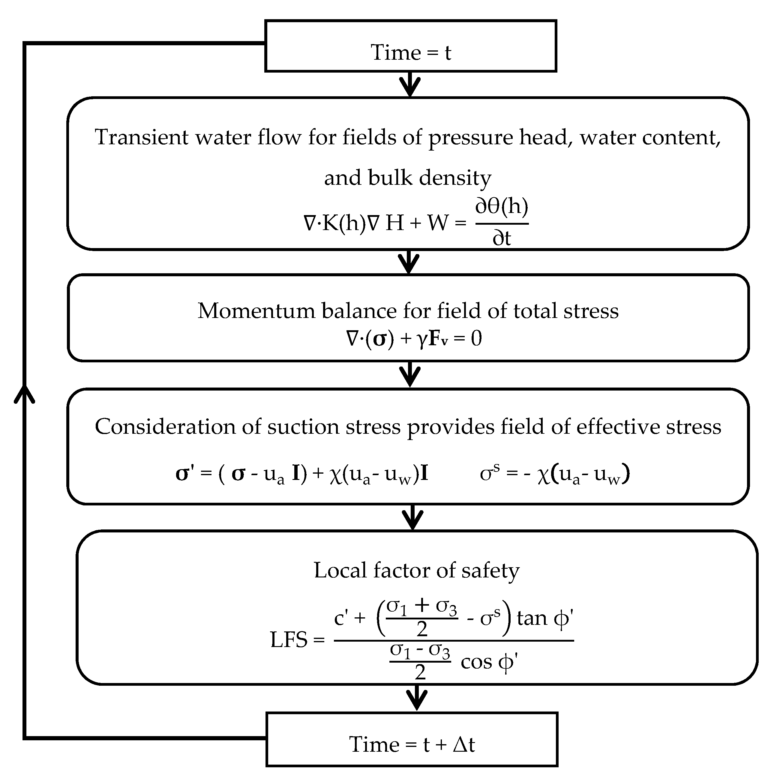
The coupled hydromechanical framework used in this study is based on Lu et al. [30] and is summarized in Figure 1. The key elements of the framework are briefly described below and the reader is referred to Lu et al. [30] for more information. The Richards’ equation [42] is used to describe changes in volumetric water content, θ [-], as a function of time, t [T].
where H [L] is the total or hydraulic head, W [T−1] represents sinks (negative) or sources (positive) of water, θ(h) [-] is the soil water retention function, and K(h) [LT−1] is the hydraulic conductivity function, which are both nonlinear functions of pressure head, h [L]. In this study, two parametric approaches are used to describe the soil water retention and the hydraulic conductivity function. The first approach is based on Mualem [43] and van Genuchten [44]. In this case, the water retention curve is given by the equation below.
where Se [-] is the effective saturation, θs [-] and θr [-] are the saturated and residual soil water content, n [-] and m (=1 − 1/n) are parameters that depend on soil pore size distribution (n is larger for more uniform pore size distribution), and α [L−1] represents the inverse of the air entry suction (larger for coarser material). The hydraulic conductivity function is given by the equation below.
where Ks [LT−1] is the saturated hydraulic conductivity and l [-] is a tortuosity parameter estimated by Mualem [43] to be about 0.5. The second parametric approach is based on Brooks and Corey [45]. In this scenario, the water retention curve is described by Equation (4) below.
where [L−1] is the air entry pressure head and [-] is the soil pore size distribution index. The hydraulic conductivity function of this approach is given by the formula below.
where [-] is a parameter that depends on the tortuosity.
In order to describe the stress distribution in the subsurface, the linear moment equilibrium for linear-elastic materials is used [30,46].
where σ [ML−1T−2] is the total stress tensor with three and six independent stress variables in 2D and 3D, respectively, γ [ML−2T−2] is the wet unit weight of the soil, and Fv [-] is the body force vector [47] with two or three components for 2D and 3D space, respectively. Here, bold characters indicate the tensorial nature of these variables. For linear-elastic materials, only Young’s (elastic) modulus, E, and Poisson’s ratio, ν, are needed to solve the field of total stress. Once the total stress and pore pressure are defined, the effective stress can be calculated. The generalized effective stress in variably saturated soils is given by Bishop [48] as seen below.
where σ′ [ML−1T−2] is the effective stress tensor, ua [ML−1T−2] is the pore air pressure, uw [ML−1T−2] is the pore water pressure, χ is the Bishop’s parameter or the effective stress parameter, and I is the unit vector. The second term in Equation (7) represents the suction stress, σs [ML−1T−2], which is always compressive for soils [49], and was first described by Lu and Likos [24] as:
Suction stress is a result of active forces at or near inter-particle contacts that keep the soil particles together. This stress can vary from a few kPa in sands to several hundred kPa in silts and clays. In this study, we have relied on the suction stress equation proposed by Lu et al. [50] where Bishop’s parameter was defined as the effective degree of saturation.
This equation is only one of the (approximate) expressions proposed in the literature to evaluate the effect of suction on the effective stress of soil. Alternative formulations are available [49]. In summary, the coupled hydromechanical model used in this study considers the body load associated with the self-weight of the slope materials, which is directly linked to dynamic variations in soil water content due to infiltration, and it considers the effective stress, which is affected by dynamic pressure head variations associated with subsurface flow. In the next step, the transient changes in hydrology and the resulting dynamical changes in stress distribution are used to assess slope stability.
The Factor of Safety (FS) is an established indicator to express the stability of a hillslope [51]. The FS is defined as the ratio between maximum retaining forces and driving forces and is calculated from the ratio of resisting shear strength τ* [ML−1T−2] to gravitationally driven shear stress, τ [ML−1T−2]. Following a similar argument, Lu et al. [30] defined the Local Factor of Safety (LFS) as the ratio of Coulomb stress for the potential failure state (τ*) and the Coulomb stress for the current state of stress (τ) under the Mohr-Coulomb criterion. For a linear elastic material, the shear strength and, thus, the Mohr-Coulomb failure envelope are defined by the formula below.
where c′ [ML−1T−2] is the effective soil cohesion and ϕ′ [°] is the effective friction angle. At each location with a specific state of effective stress, the LFS can then be calculated from the triangles ABC and ADE shown in Figure 2 as:
where σI′ and σII′ [ML−1T−2] are the midpoint and radius of the Mohr circle, respectively, which are calculated by the equation below.
where σ1 and σ3 [ML−1T−2] are the major and minor principal total stresses, respectively. When the Mohr circle is shifted leftward as a result of increasing soil water content (i.e., a reduction in soil suction), this may reduce the LFS to less than unity, which indicates unstable conditions and potential land sliding [6,30].
τ* = c′ + σ′ tan ϕ′
In this study, the distribution of the LFS as a response to spatio-temporal variation in soil water content and suction will be analyzed and the temporal development of connected areas with LFS < 1 will be interpreted as the development of potentially unstable and failure-prone areas. This interpretation strategy has been applied in several earlier studies [30,35]. Nevertheless, it is important to note some limitations of the LFS method in this case. Clearly, the LFS method only relies on the shear stress magnitude at each point within a hillslope independent from the neighboring elements and the shear stress tensors. In fact, the value of LFS that is calculated with Equation (11) for each point of the slope refer to a differently inclined plane along which the shear stress is calculated (Figure 3). This plane is orthogonal to the plane of the principal stresses (σ1 and σ3) and its trace forms an angle (β) with σ3 where:
The orientation of this plane depends on the direction of the total stress principal components, which may change from point to point (and from time to time) for a variably saturated slope. It is important to realize that enhancing or diminishing effects of the shear stress tensors of the neighboring elements are ignored. Therefore, areas with LFS < 1 do not necessarily lead to failure. This becomes even more complicated when studying 3D slopes with more stress tensors in different directions. Moreover, the LFS method is only valid for linear elastic materials and, thus, does not consider the readjustment of the stress distribution within a slope after failure. Therefore, it is strictly taken as not appropriate to approximate areas with LFS < 1 with the development of a potential failure surface. Despite these obvious simplifications, Lu et al. [30] showed that the results of stability analysis based on the LFS method are in general agreement with results obtained with conventional methods while providing better opportunities to investigate coupling of hydrological and mechanical processes.
3. Materials and Methods
3.1. Set-Up of the Benchmark Model
The coupled hydromechanical framework has been implemented in COMSOL Multiphysics (COMSOL Inc, Stockholm, Sweden), which facilitates coupling of flow and transport and mechanical processes in porous media. In a first step, a set of 2D and 3D benchmark simulations was performed. For this, the 30° slope and silty soil of Lu et al. [30] were used with the model parameters provided in Table 1 (Figure 4). The 3D model extended 10 m in the z-direction (Figure 4b). Following Lu et al. [30], the Mualem-van Genuchten functions were used to describe the water retention and hydraulic conductivity of the slope. The entire domain of this benchmark simulation is homogeneous and considered to be in hydrostatic equilibrium with a ground water table at a depth of 15 m initially. At the surface, an infiltration boundary condition is used and the remaining lateral and bottom boundaries are no-flow boundaries.
The selection of appropriate boundary conditions for the mechanical model plays an important role for the distribution and development of internal stresses of a slope [52,53]. In field applications, they should be carefully selected based on the condition that best matches reality. In this synthetic modeling study, it is assumed that there is no displacement in the normal direction for the bottom and lateral boundaries of the model domain (i.e., so-called roller boundary conditions). For the 3D simulations, roller boundary conditions were also used for the side end faces of the model. This implies that there is no in-plane shear restraint and the effect of shear resistance is removed for the two faces [52,53]. With this choice of boundary conditions, the 2D and 3D stress distributions are expected to match for homogenous 2D and 3D slopes with identical water content and pressure head distribution. Moreover, there is no load or constraint implemented on the slope surface and, therefore, it is considered to be a free boundary. This model set-up provides the best opportunity to compare the effect of transient water content distribution on the stability in 2D and 3D simulations with the coupled hydromechanical framework. To reduce the effect of the boundary conditions on all stability assessments, the computation domain was, nevertheless, extended considerably beyond the area of interest (see Figure 4). In the following information, all results are reported for only a part of the simulation domain (i.e., the control area), which is indicated by the dark grey area in Figure 4.
The 2D and the 3D simulation domains were discretized using an increasing mesh size with an increasing distance from the soil surface (Figure 4a). This is because of the highly dynamic hydrological response near the soil surface due to infiltration, which requires a fine discretization. Deeper in the subsurface, hydrological conditions are less dynamic and a coarser discretization can be used. In this way, the computational efficiency was increased without a negative effect on the accuracy of the modeling results [6,30,54].
3.2. Numerical Experiments
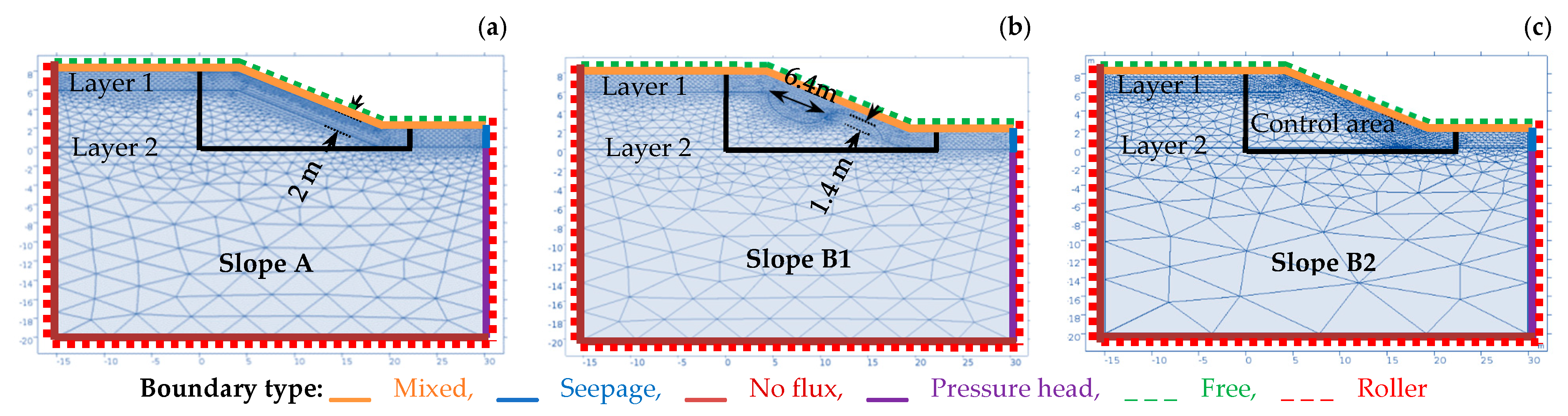
In order to study the effect of variable bedrock topography, a two-layer slope was created that represents less permeable bedrock covered by a 2 m thinner and more permeable sandy loam layer. The general properties of the slope and soil layers are based on the study of Shao et al. [35] and are summarized in Table 2. In this set of simulations, the Brooks-Corey functions for water retention and hydraulic conductivity were used as in Shao et al. [35]. Three different bedrock topographies were considered for 2D simulations (Figure 5). Slope A has an equal soil layer depth along the slope while slope B1 and B2 have variable bedrock topography. In order to magnify the effect of bedrock topography, a rather simple and extreme bedrock surface with only two features was used. One feature represented areas with shallow bedrock and a thin soil layer and the second feature represented bedrock depressions with a thicker soil. The difference between slope B1 and B2 is the position of these two features where shallow bedrock is positioned downslope in slope B1 and upslope in slope B2. In all three slopes, the overall area and, thus, the storage volume of each layer was the same.
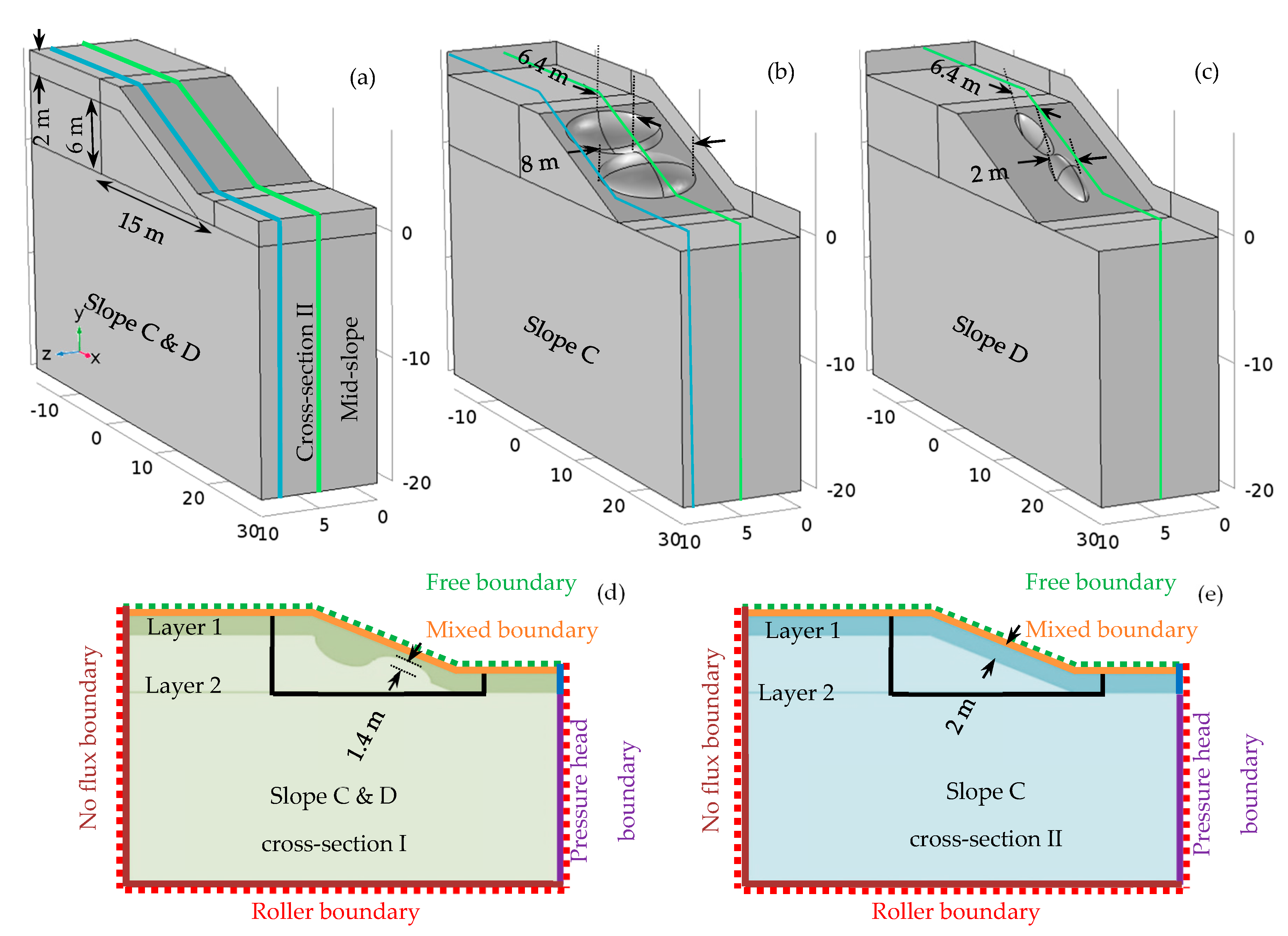
In the next step, one of the 2D slopes with variable bedrock topography (slope B1) was extended to a 3D slope. For this reason, two different scenarios were considered (slope C and D, Figure 6). For slope C and D, the mid-cross sections along the length of the slopes (see mid-slope cross-section I in Figure 6) were the same as for slope B1. However, the extension of the features in the z-direction was larger for slope C than for slope D. As in the case of slope B1, the upper feature represented a bedrock depression while the lower feature represented a bedrock outcrop.
To obtain more realistic initial conditions compared to the benchmark model, a spin-up period of 10 years with a constant low-intensity rainfall of 600 mm per year was used. The resulting water content and pressure head distributions were then used as the initial condition for the simulation of rainfall events [35]. In this study, two different event rainfalls with the same precipitation amount but different intensity were implemented to study the effect of soil layering and bedrock topography on slope stability. The first simulated rainfall event was a high-intensity event (relative to Ks) with 20 mm per hour for 15 h and the second rainfall event was a low-intensity event with 2 mm per hour for 150 h. The high intensity is about 77% of the Ks of the top layer while the low intensity is 7.7% of this Ks. However, both rainfall intensities are higher than the Ks of the bottom (bedrock) layer. In the following calculations, these two rainfall events are implemented on slope A, B1, and B2 and the results are compared. For comparing the 2D and 3D simulations, the high-intensity rainfall event was used. The boundary conditions in these numerical experiments were slightly modified relative to the benchmark model. In these cases, water can flow out of the slopes’ domain through the upper-right side boundary (seepage boundary in Figure 6d,e). Moreover, the top boundaries are defined to be mixed boundaries where rainfall is infiltrated until the pore water pressure exceeds the pore air pressure after which water can flow out of the surface similar to a seepage face. The water leaving the domain in this way will be referred to as surface run-off even though it is important to realize that we are not using a coupled surface-subsurface flow model and that surface routing and re-infiltration are, thus, not considered here.
The computation time associated with the numerical experiments presented in these cases was substantial because COMSOL Multiphysics aims for convenience of model coupling but not for optimal numerical performance. For the selected discretizations, the 2D simulations presented in this study typically took only a few minutes when the soil surface was not saturated but increased dramatically afterwards. The simulation time for the case of 3D slopes was much longer (on the order of days) and it was found that performance was very sensitive to the model discretization. Clearly, there are still considerable challenges associated with 3D hydromechanical modeling. This can certainly be improved by using tailored instead of general-purpose software for hydromechanical modeling.
4. Results and Discussion
4.1. Results for the Benchmark Model
The simulated LFS for the 2D and 3D implementation of the coupled hydromechanical model in COMSOL for the benchmark model are shown in Figure 7. It can be seen that the 2D implementation (Figure 7b) matches well with the previously published results of Lu et al. [30] (Figure 7a) especially near the surface where it is most relevant for slope stability assessment. The results of the 3D implementation of the LFS concept are presented in Figure 7c and a mid-slope cross-section is provided in Figure 7d. The results for the cross-section of the 3D model and the 2D model agree very well, which verifies this first 3D implementation of the LFS concept. As expected, no variation in the z-direction was observed for the selected mechanical boundary conditions. It is important to note that LFS tends to decrease with a greater depth in both 2D and 3D simulations. This is a consequence of the Mohr-Coulomb description of linear elastic materials and is due to reduction in the contribution of effective cohesion in soil shear strength while the total stress grows with depth and the frictional term becomes greater (see Equations (10) and (11)). The limit value of LFS at an infinite depth for slopes with no external load and no tectonic stresses can be obtained from Equation (11).
For the values of ν and ϕ′ used in this study (see Table 1 and Table 2), the limit value of LFS does not go below the stability threshold of LFS ≤ 1. Nevertheless, the focus in this study will be on the temporal development of the near-surface LFS distribution since this is where hydrology is expected to affect slope stability. In the following sections, both the 2D and 3D implementation of the LFS concept will be used to explore the effect of layer depth on the stability assessment of variably saturated hillslopes in response to different types of rainfall events.
4.2. Results of the 2D Numerical Experiments
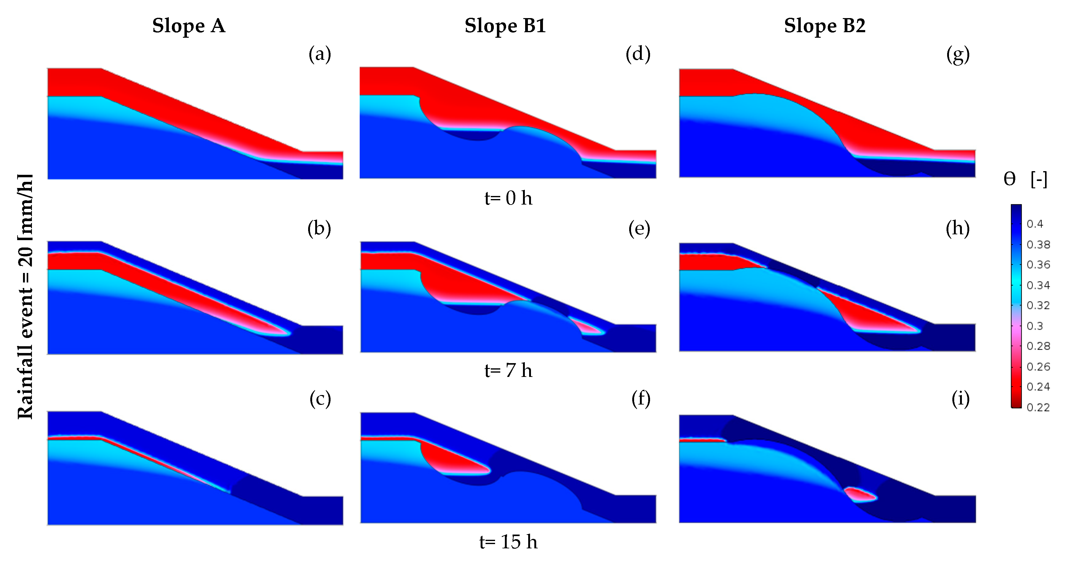
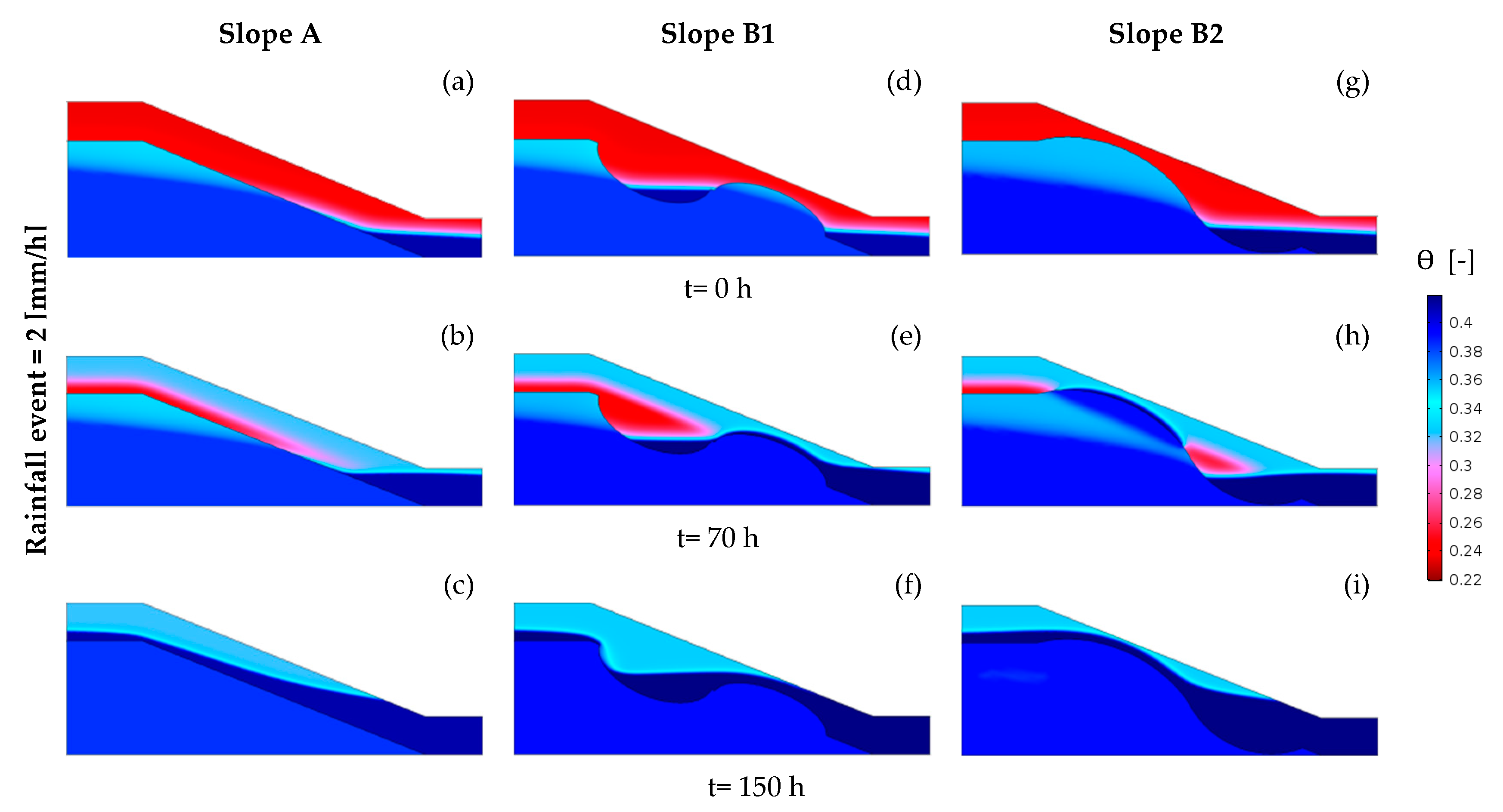
Figure 8 and Figure 9 present the dynamical development of the soil water content distribution in slope A, B1, and B2 during the high-intensity and the low-intensity rainfall event, respectively. In these two figures, the distributions at t = 0 h show the initial water content distribution for the event rainfall after a spin-up period with 20 years of long-term rainfall of 600 mm per year. It can be seen that the saturated area extended into the top layer at the toes of all of the slopes. In the slopes with variable soil thickness, saturated conditions also occurred in the bedrock depressions. In the case of the high-intensity rainfall event, the fully saturated area at the slope toe of slope A gradually developed and extended upward along the slope (Figure 8a–c). The soil water content of slope A developed in a similar manner for the low-intensity rainfall event. However, a more clearly defined perched water table developed after the infiltrated water reached the bedrock, which suggests that lateral flow plays a more important role in this case. Due to the more complex bedrock topography, the soil water content distribution developed differently in slope B1 and B2. In the case of the high-intensity event, fully saturated areas in the upper layer of these slopes were established faster and appeared both on the slopes toe as well as above the bedrocks with a thin soil layer. These fully saturated areas then grew upward and downward until the entire slopes were saturated (Figure 8d–i). In the case of the low-intensity event, infiltrated water was redistributed more strongly along the bedrocks interface. Therefore, the areas with thin soil did not saturate earlier than other parts of the slopes, which were observed for the high-intensity rainfall (Figure 9i). The difference between slope B1 and B2 was more pronounced for the low-intensity rainfall. In particular, the perched groundwater table associated with the shallow bedrock near the slope toe in case of slope B1 reached the surface and created a larger saturated area than in the case of slope B2.
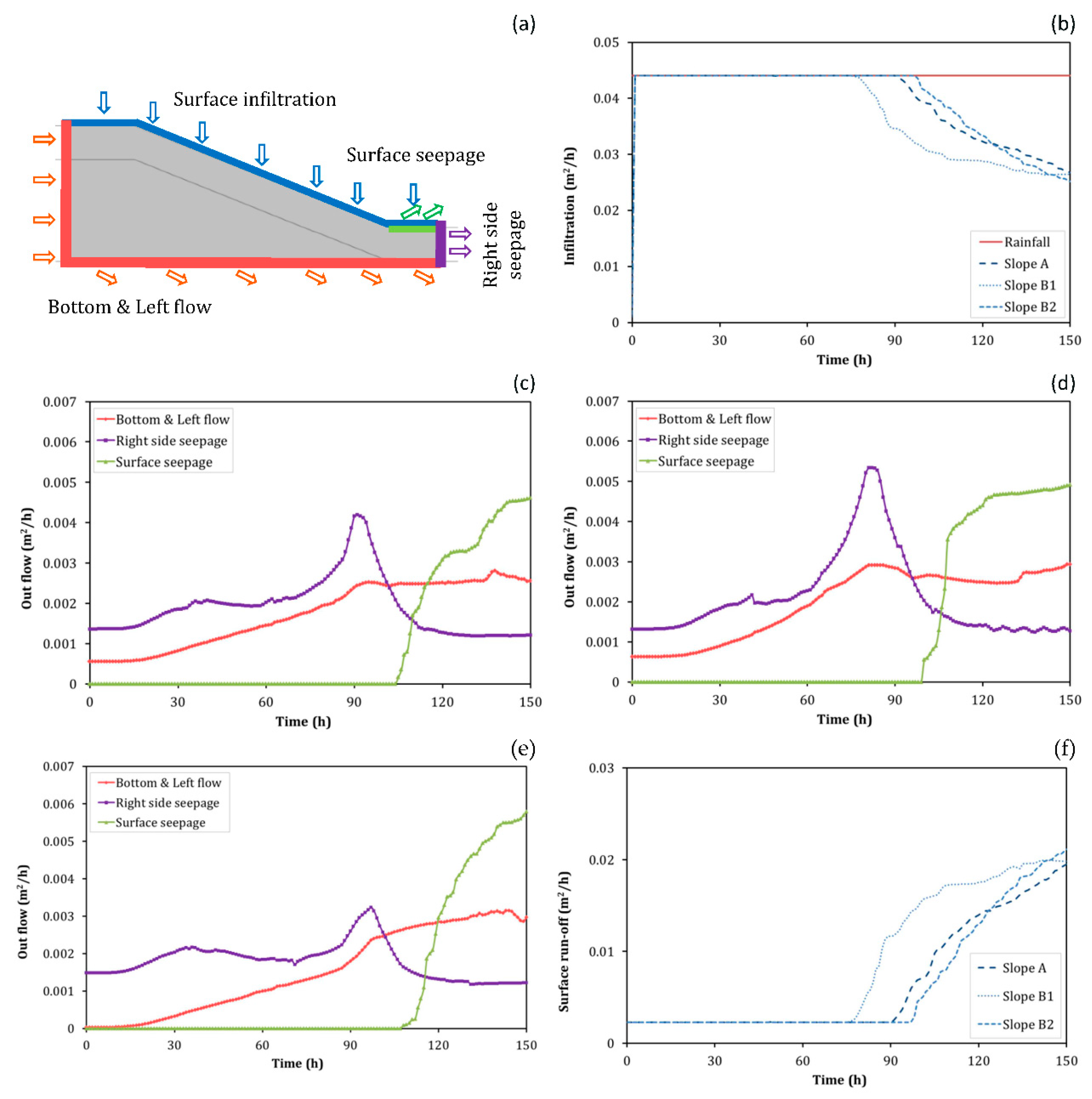
Figure 10 and Figure 11 present the net fluxes into and out of the control area through different boundaries of the model domain for the different slopes and the two rainfall intensities. In the case of the high-intensity rainfall, the net infiltration (inflow−outflow, Figure 10b) along the surface boundary matched the rainfall rate at the start of the simulation. It can also be seen that the infiltration rate for slope A reduced later than for the slopes with variable soil thickness so that the total amount of infiltration was higher for slope A. The difference between the net infiltration and rainfall converts to surface run-off (Figure 10f). Figure 10 also shows that the maximum seepage rate from the right side boundary was larger for slope A but started to increase later when compared to the other two slopes. The outflow from the bottom and left side boundaries of the control area behaved in a similar manner. The difference in the timing of reduced infiltration and the start of the increased outflow is consistent with the water content distribution presented in Figure 8 where saturation occurred earlier and in a larger area of the slopes with a variable soil thickness. The earlier saturation prevented more infiltration and this explains the lower seepage and outflow rates and cumulative amounts for slope B1 and B2. For the case of the low intensity rainfall (Figure 11), the differences in boundary fluxes are much less pronounced. However, the larger extent of the saturated area due to the shallow bedrock near the slope toe in slope B1 resulted in an earlier reduction of net infiltration (Figure 11b) and an earlier surface seepage (Figure 11d).
In summary, these simulations show that bedrock topography and soil layering define the groundwater level and the water content distribution of the soil and, thus, the saturation-prone areas along the slopes. However, the position and extent of the saturated areas was found to depend strongly on the rainfall intensity. The part of the slopes with thinner soil tended to get saturated earlier than other parts of the slopes in the case of high-intensity rainfall due to the dominance of vertical flow. For low-intensity rainfall, lateral redistribution of water played a more important role and areas with shallow bedrock did not saturate earlier than other parts of the slopes. The increased importance of lateral flow also resulted in a higher sensitivity to the position of bedrock features along the slopes.
The difference in the water content development of the 2D slopes also resulted in different LFS predictions. The temporal evolution of the LFS for these slopes is shown in Figure 12 and Figure 13 for the high-intensity and low-intensity rainfall event, respectively. The black contour lines indicate the near-surface zone with an LFS below 1. It can be seen in Figure 12 that the shape and location of the potentially unstable zone were different in slope A, B1, and B2 for the high-intensity rainfall. The potential time of failure initiation was also earlier for slope B1 and B2. In slope A with constant soil thickness, the failure prone zone developed from the slope toe and expanded upward with an increasing water content of the top layer. In contrast, the failure-prone zones of slopes with variable bedrock topography initiated directly within regions with shallow soil as well as the slope toe where high saturation and pore water pressure appeared first. The potential failure area with LFS < 1.0 was higher for slope B1 and B2 than for slope A at all times of the intensive rainfall event even though the overall area of the top soil layer and soil water storage was the same in all slopes. These simulation results clearly illustrate that bedrock topography influenced the water content development and stress distribution. In particular, the vulnerable zone appeared faster in the slopes with variable bedrock topography and occurred at locations associated with a thin soil cover. For the low intensity rainfall, the lateral redistribution of subsurface flow played a more important role and provided a rather similar water content distribution along the slopes surfaces that consequently resulted in a similar size and position of failure-prone areas in all three slopes. In this scenario, the potential failure zone initiated and developed at the slopes toe and the depth to bedrock did not strongly influence this area. Comparing the area of the potential failure zone for each slope (see Figure 12 and Figure 13) shows that, for the same amount of rainfall, the more intensive rainfall (20 mm per hour) caused a bigger unstable zone, which is consistent with the results of Schiliro et al. [17]. However, in contrast to previous studies [36], these simulation results suggest that instability is not initiated in bedrock macro-topographic depressions. The more intensive rainfall first influenced the pore pressure of the near surface areas and areas with shallow soil and the vulnerable zones expanded into the area with bedrock depressions from this region. Less intensive rainfall resulted in more dominant lateral flow along the bedrock interface, which disconnected the occurrence of failure-prone zones from the bedrock topography. Preferential flow was not considered in this case. We anticipate that the main findings presented here would be similar if preferential flow is assumed to be prevalent along the entire hillslopes (as in Shao et al. [35]). However, if preferential flow mainly occurs in areas with bedrock depressions and would be able to directly bypass the soil and reach the bedrock quickly, this could have a significant impact on the results presented in this paper.
4.3. Results of the 3D Numerical Experiments
Figure 14 compares the simulated water content distribution for the 2D slope with a variable layer thickness (slope B1) with the mid-slope cross-sections of the two 3D slopes (slope C and D). It can be seen that the initial extent of the saturated area obtained after a spin-up period is highest in the 2D slope B1 (Figure 14a, t = 0) while the extent of the saturated area at t = 0 h is lowest in Slope D with the smaller-sized bedrock depression (Figure 14g). After the start of the high-intensity rainfall event, the top layer was saturated first in the region with a shallow bedrock for all three slopes. However, the fully saturated area appeared first in the 2D model (slope B1), which was followed by slope C and D, respectively. Figure 15 compares the simulated water content distribution for slope A and cross-section II of slope C (see Figure 5a). Although the initial water content distribution at t = 0 h is nearly the same, the saturated area appeared faster and showed a larger extent in the cross-section of slope C. The magnitude of the fluxes through the boundaries of the control area of Slope B1 and D, which showed the biggest differences in water content development, are presented in Figure 16. Infiltration into the control area of slope B1 started to decrease earlier than for slope D and the total amount of infiltration is smaller for slope B1. In addition, seepage from the surface and outflow from the other boundaries of the control area started earlier in slope B1. Since less water was infiltrated into the saturated slope B1 (Figure 16b), the overall amount of outflow is lower than for slope D. These differences are related to the fact that water can flow around the convex bedrock outcrop in the 3D simulations, which is clearly not possible in the 2D model. The lack of flow divergence in the 2D slope caused the control area of slope B1 to saturate faster, which caused more flow out of the control area. For the 3D simulations, the flow divergence around the bedrock outcrop caused an increase in the extent of the saturated area in cross-section II.
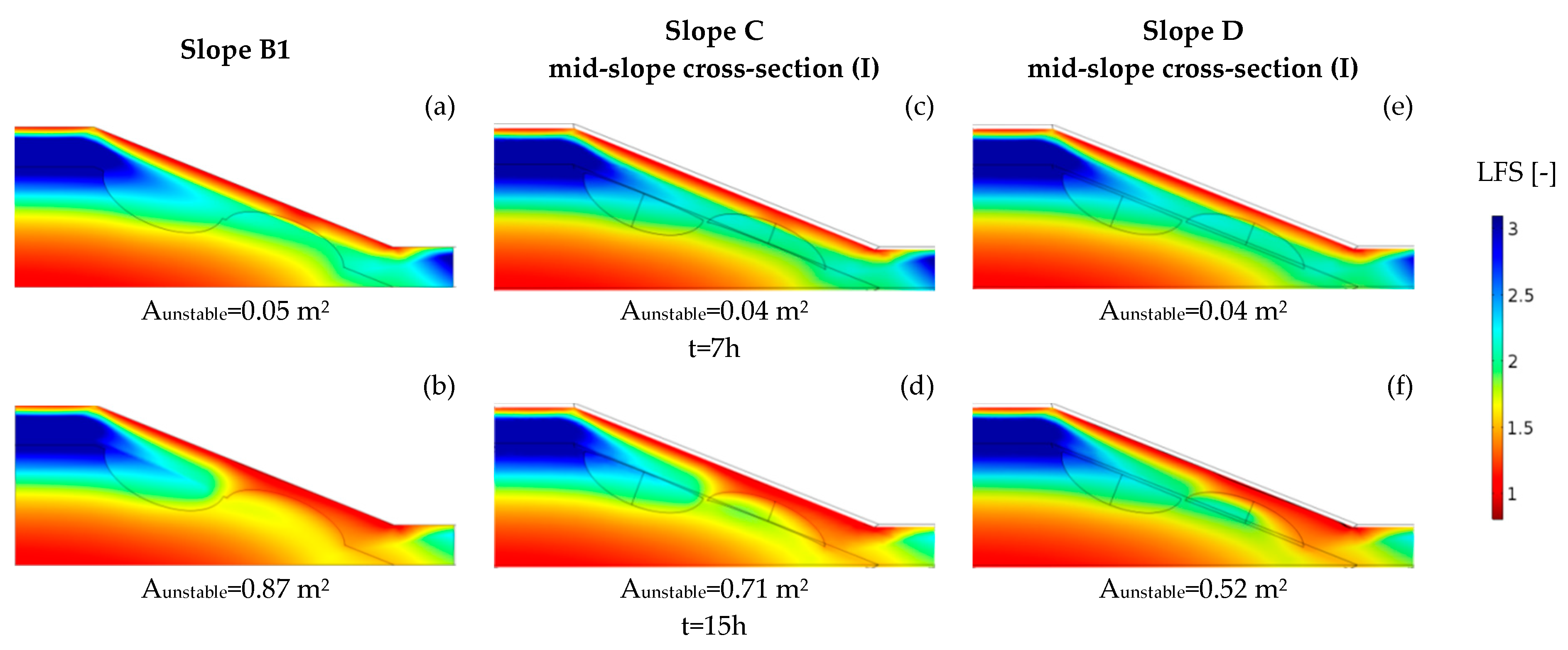
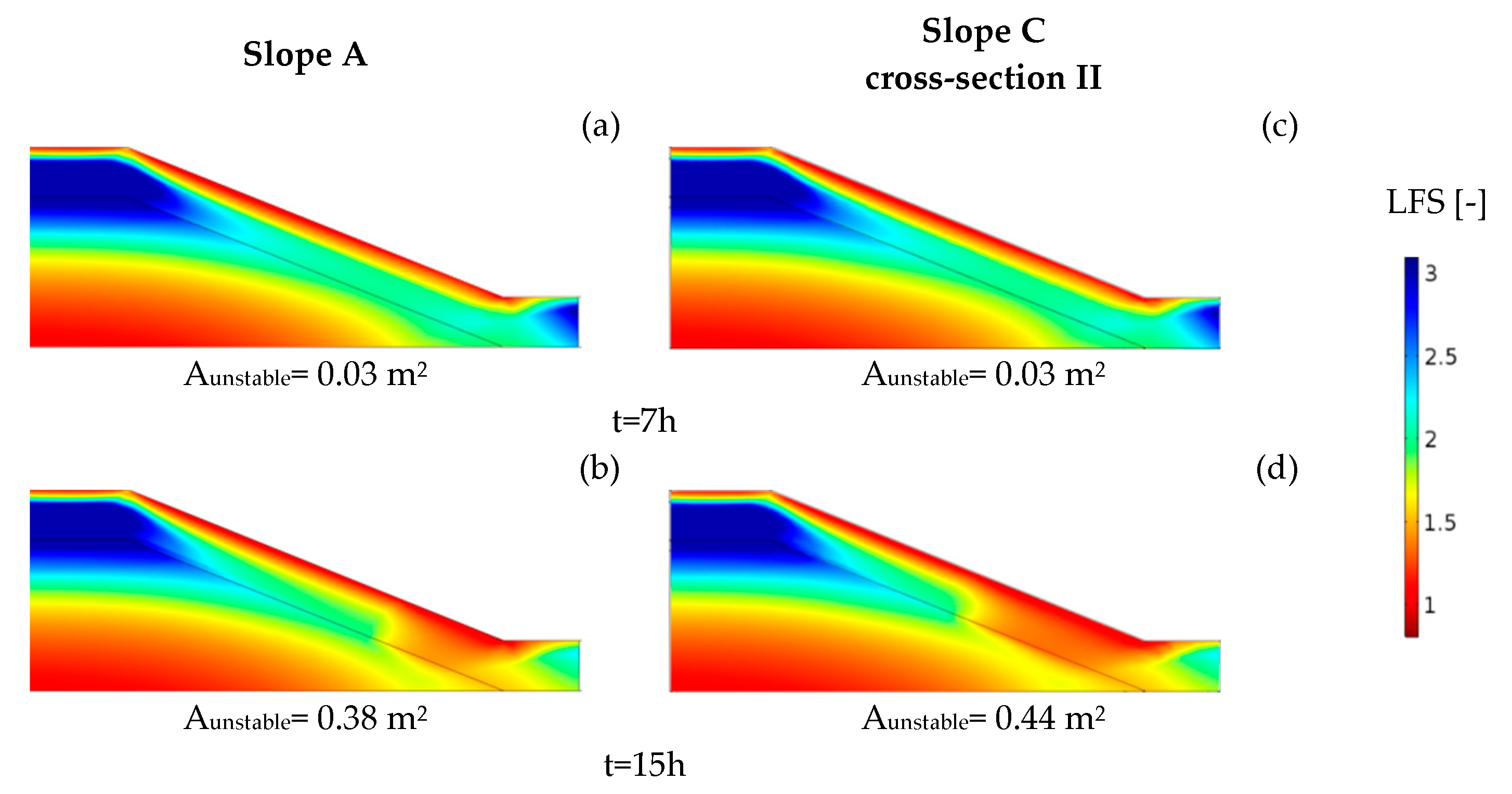
In Figure 17, the predicted LFS of the 2D slope B1 and the mid-slope cross-section I of the 3D slopes C and D are compared. It can be seen that the most vulnerable zones appeared first above the shallow bedrock for all three slopes as well as at the slope toe. In terms of timing, the vulnerable zones initiated first in the 2D slope B1 and afterwards in slope C and in slope D. The extent of the unstable area at the end of the intensive rainfall (t = 15 h) was also the largest for the 2D slope B1. It is also of interest to compare the development of the LFS distribution for the 2D slope A and cross-section II of the 3D slope C (Figure 18). In this scenario, it can be seen that flow divergence in the 3D model led to a larger unstable area when compared to the 2D model. These results clearly show how 2D and 3D simulations of hydromechanical processes may result in different stability assessments depending on the slope morphology and layering within the soil domain. However, the stability of actual 3D slopes may be higher than shown here because of the importance of the mechanical boundary conditions for the end faces in the z-direction. In addition, the direction of the shear stress tensor has not been considered in this case and could lead to additional differences in failure surfaces for 2D and 3D models.
5. Conclusions
Slope stability is governed by coupled hydrological and mechanical processes. Most available models describing these coupled hydro-mechanical processes either rely on 1D or 2D representations of hydrological and mechanical properties and processes, which is a strong simplification in many applications. In this study, both 2D and 3D coupled hydromechanical models using the local factor of safety concept were implemented in COMSOL Multiphysics. These coupled models were used to study the effect of bedrock topography on the subsurface flow and the resulting stability of hillslopes for different rainfall intensities. The simulation results for 2D slopes with constant and variable bedrock topography showed that bedrock topography is an important control on the spatial and temporal distribution of the potentially unstable zones and that the importance of bedrock topography increases with rainfall intensity. In particular, simulations with a high rainfall intensity showed that potential failure zones developed faster in slopes with variable bedrock topography and were initiated in areas that saturated earlier (i.e., at the slope toe and regions with a thinner soil). In the case of low-intensity rainfall events, lateral flow played a more important role and the position of potentially unstable areas was disconnected from the bedrock topography and occurred mainly at the slope toe. These results clearly highlight the importance of considering the interactions between bedrock topography and slope hydrological processes in slope stability evaluations.
In the next step, 2D and 3D simulations were compared for the case of high-intensity rainfall. In this scenario, it was found that the position of bedrock features along the slopes as well as slopes width (in 3D models) and the topography of the surrounding bedrock can have a considerable impact on the development of the soil water content and, therefore, the stability of that specific point. For example, water flow around a zone of shallow bedrock or the amount of collected water in a bedrock depression for a specific amount of rainfall will depend on the size of the inhomogeneity in three dimensions. Overall, we believe that the importance of 3D simulations of slope stability increases for more complex geometries. There also are more challenging aspects to 3D simulations with coupled hydromechanical models. In particular, the need for a spatial discretization with a high resolution near the soil surface leads to much longer simulation times when compared to 2D simulations. Another issue is the proper selection of the mechanical boundary condition at the side faces in the third dimension, which may substantially affect predicted slope stability. Lastly, the general value of the local factor of safety method is still under debate because of concerns about neglecting the inherent tensorial nature of the stress field and this should be investigated in more detail in future studies.
Author Contributions
Conceptualization, S.M. and J.A.H.; Methodology, S.M., J.A.H. and H.C.; Software, S.M.; Resources, J.A.H. and H.V.; Writing-Original Draft Preparation, S.M.; Writing-Review & Editing, S.M., J.A.H., H.C. and H.V.; Visualization, S.M.; Supervision, J.A.H., H.C. and H.V.; Project Administration, J.A.H. and H.V.; Funding Acquisition, J.A.H. and H.C.
Funding
This research was funded by the German Ministry of Education and Research (BMBF) in the framework of the R&D Program GEOTECHNOLOGIEN through the project ‘Characterization, monitoring and modelling of landslide-prone hillslopes (CMM-SLIDE)’ (grant number 03G0849A).
Acknowledgments
We thank the three anonymous reviewers and the associate editor for the constructive reviews that improved the quality of this manuscript.
Conflicts of Interest
The authors declare no conflicts of interest.
References
- Cuomo, S.; Della Sala, M. Large-area analysis of soil erosion and landslides induced by rainfall: A case of unsaturated shallow deposits. J. Mt. Sci. 2015, 12, 783–796. [Google Scholar] [CrossRef]
- Cuomo, S.; Della Sala, M. Rainfall-induced infiltration, runoff and failure in steep unsaturated shallow soil deposits. Eng. Geol. 2013, 162, 118–127. [Google Scholar] [CrossRef]
- Borja, R.I.; White, J.A. Continuum deformation and stability analyses of a steep hillside slope under rainfall infiltration. Acta Geotech. 2010, 5, 1–14. [Google Scholar] [CrossRef]
- Crosta, G.B.; Frattini, P. Rainfall-induced landslides and debris flows—Preface. Hydrol. Process. 2008, 22, 473–477. [Google Scholar] [CrossRef]
- Matsushi, Y.; Matsukura, Y. Rainfall thresholds for shallow landsliding derived from pressure-head monitoring: Cases with permeable and impermeable bedrocks in Boso Peninsula, Japan. Earth Surf. Process. Landf. 2007, 32, 1308–1322. [Google Scholar] [CrossRef] [Green Version]
- Lu, N.; Wayllace, A.; Oh, S. Infiltration-induced seasonally reactivated instability of a highway embankment near the Eisenhower Tunnel, Colorado, USA. Eng. Geol. 2013, 162, 22–32. [Google Scholar] [CrossRef]
- Godt, J.W.; Baum, R.L.; Lu, N. Landsliding in partially saturated materials. Geophys. Res. Lett. 2009, 36. [Google Scholar] [CrossRef] [Green Version]
- Keefer, D.K.; Larsen, M.C. Assessing landslide hazards. Science 2007, 316, 1136–1138. [Google Scholar] [CrossRef] [PubMed]
- Petley, D.N. On the impact of climate change and population growth on the occurrence of fatal landslides in South, East and SE Asia. Q. J. Eng. Geol. Hydrogeol. 2010, 43, 487–496. [Google Scholar] [CrossRef]
- Klose, M.; Maurischat, P.; Damm, B. Landslide impacts in Germany: A historical and socioeconomic perspective. Landslides 2016, 13, 183–199. [Google Scholar] [CrossRef]
- Sidle, R.C.; Ochiai, H. Landslides: Processes, Prediction and Land Use; American Geophysical Union: Washington, DC, USA, 2006. [Google Scholar]
- Lu, N.; Godt, J.W. Hillslope Hydrology and Stability; Cambridge University Press: New York, NY, USA, 2013. [Google Scholar]
- Montgomery, D.R.; Dietrich, W.E. A physically-based model for the topographic control on shallow landsliding. Water Resour. Res. 1994, 30, 1153–1171. [Google Scholar] [CrossRef]
- Kim, M.S.; Onda, Y.; Kim, J.K.; Kim, S.W. Effect of topography and soil parameterisation representing soil thicknesses on shallow landslide modelling. Quat. Int. 2015, 384, 91–106. [Google Scholar] [CrossRef]
- Lehmann, P.; Or, D. Hydromechanical triggering of landslides: From progressive local failures to mass release. Water Resour. Res. 2012, 48. [Google Scholar] [CrossRef] [Green Version]
- Gabet, E.J.; Dunne, T. Landslides on coastal sage-scrub and grassland hillslopes in a severe El Nino winter: The effects of vegetation conversion on sediment delivery. Geol. Soc. Am. Bull. 2002, 114, 983–990. [Google Scholar] [CrossRef]
- Schiliro, L.; Esposito, C.; Mugnozza, G.S. Evaluation of shallow landslide-triggering scenarios through a physically based approach: An example of application in the southern Messina area (northeastern Sicily, Italy). Nat. Hazards Earth Syst. Sci. 2015, 15, 2091–2109. [Google Scholar] [CrossRef]
- Peres, D.J.; Cancelliere, A. Estimating return period of landslide triggering by Monte Carlo simulation. J. Hydrol. 2016, 541, 256–271. [Google Scholar] [CrossRef]
- Stahli, M.; Sattele, M.; Huggel, C.; McArdell, B.W.; Lehmann, P.; Van Herwijnen, A.; Berne, A.; Schleiss, M.; Ferrari, A.; Kos, A.; et al. Monitoring and prediction in early warning systems for rapid mass movements. Nat. Hazards Earth Syst. Sci. 2015, 15, 905–917. [Google Scholar] [CrossRef] [Green Version]
- Lehmann, P.; Gambazzi, F.; Suski, B.; Baron, L.; Askarinejad, A.; Springman, S.M.; Holliger, K.; Or, D. Evolution of soil wetting patterns preceding a hydrologically induced landslide inferred from electrical resistivity survey and point measurements of volumetric water content and pore water pressure. Water Resour. Res. 2013, 49, 7992–8004. [Google Scholar] [CrossRef] [Green Version]
- Srinivasan, K.; Howell, B.; Anderson, E.; Flores, A. A low cost wireles sensor network for landslide hazard monitoring. In Proceedings of the 2012 IEEE International Geoscience and Remote Sensing Symposium, Munich, Germany, 22–27 July 2012; pp. 4793–4796. [Google Scholar]
- Terzaghi, K. Theoretical Soil Mechanics; Wiley: New York, NY, USA, 1943. [Google Scholar]
- Eichenberger, J.; Ferrari, A.; Laloui, L. Early warning thresholds for partially saturated slopes in volcanic ashes. Comput. Geotech. 2013, 49, 79–89. [Google Scholar] [CrossRef] [Green Version]
- Lu, N.; Likos, W.J. Suction stress characteristic curve for unsaturated soil. J. Geotech. Geoenviron. Eng. 2006, 132, 131–142. [Google Scholar] [CrossRef]
- Godt, J.W.; Sener-Kaya, B.; Lu, N.; Baum, R.L. Stability of infinite slopes under transient partially saturated seepage conditions. Water Resour. Res. 2012, 48. [Google Scholar] [CrossRef] [Green Version]
- Baum, R.; Godt, J. Early warning of rainfall-induced shallow landslides and debris flows in the USA. Landslides 2010, 7, 259–272. [Google Scholar] [CrossRef]
- Raia, S.; Alvioli, M.; Rossi, M.; Baum, R.L.; Godt, J.W.; Guzzetti, F. Improving predictive power of physically based rainfall-induced shallow landslide models: A probabilistic approach. Geosci. Model Dev. 2014, 7, 495–514. [Google Scholar] [CrossRef]
- Arnone, E.; Noto, L.V.; Lepore, C.; Bras, R.L. Physically-based and distributed approach to analyze rainfall-triggered landslides at watershed scale. Geomorphology 2011, 133, 121–131. [Google Scholar] [CrossRef]
- Lu, N.; Godt, J. Infinite slope stability under steady unsaturated seepage conditions. Water Resour. Res. 2008, 44. [Google Scholar] [CrossRef]
- Lu, N.; Sener-Kaya, B.; Wayllace, A.; Godt, J.W. Analysis of rainfall-induced slope instability using a field of local factor of safety. Water Resour. Res. 2012, 48. [Google Scholar] [CrossRef] [Green Version]
- Hovland, H.J. Three-dimensional slope stability analysis method. J. Geotech. Eng. Div. 1977, 103, 971–986. [Google Scholar]
- Wong, F.S. Uncertainties in modeling of slope stability. Comput. Struct. 1984, 19, 777–791. [Google Scholar] [CrossRef]
- Rabie, M. Comparison study between traditional and finite element methods for slopes under heavy rainfall. HBRC J. 2014, 10, 160–168. [Google Scholar] [CrossRef]
- Hammah, R.E.; Yacoub, T.E.; Corkum, B.; Curran, J. (2005) A comparison of finite element slope stability analysis with conventional limit-equilibrium investigation. In Proceedings of the 58th Canadian Geotechnical and 6th Joint IAH-CNC and CGS Groundwater Specialty Conferences—GeoSask 2005, Saskatoon, SK, Canada, 18–21 September 2005; pp. 480–487. [Google Scholar]
- Shao, W.; Bogaard, T.A.; Bakker, M.; Greco, R. Quantification of the influence of preferential flow on slope stability using a numerical modelling approach. Hydrol. Earth Syst. Sci. 2015, 19, 2197–2212. [Google Scholar] [CrossRef] [Green Version]
- Lanni, C.; McDonnell, J.; Hopp, L.; Rigon, R. Simulated effect of soil depth and bedrock topography on near-surface hydrologic response and slope stability. Earth Surf. Process. Landf. 2013, 38, 146–159. [Google Scholar] [CrossRef]
- Freer, J.; McDonnell, J.J.; Beven, K.J.; Peters, N.E.; Burns, D.A.; Hooper, R.P.; Aulenbach, B.; Kendall, C. The role of bedrock topography on subsurface storm flow. Water Resour. Res. 2002, 38. [Google Scholar] [CrossRef]
- Tromp-van Meerveld, H.J.; McDonnell, J.J. On the interrelations between topography, soil depth, soil moisture, transpiration rates and species distribution at the hillslope scale. Adv. Water Resour. 2006, 29, 293–310. [Google Scholar] [CrossRef]
- Vereecken, H.; Huisman, J.A.; Franssen, H.J.H.; Bruggemann, N.; Bogena, H.R.; Kollet, S.; Javaux, M.; van der Kruk, J.; Vanderborght, J. Soil hydrology: Recent methodological advances, challenges, and perspectives. Water Resour. Res. 2015, 51, 2616–2633. [Google Scholar] [CrossRef] [Green Version]
- Talebi, A.; Troch, P.A.; Uijlenhoet, R. A steady-state analytical slope stability model for complex hillslopes. Hydrol. Process. 2008, 22, 546–553. [Google Scholar] [CrossRef]
- Tromp-van Meerveld, H.J.; McDonnell, J.J. Threshold relations in subsurface stormflow: 2. The fill and spill hypothesis. Water Resour. Res. 2006, 42. [Google Scholar] [CrossRef] [Green Version]
- Richards, L.A. Capillary conduction of liquids through porous mediums. J. Appl. Phys. 1931, 1, 318–333. [Google Scholar] [CrossRef]
- Mualem, Y. Hysteretical models for prediction of hydraulic conductivity of unsaturated porous-media. Water Resour. Res. 1976, 12, 1248–1254. [Google Scholar] [CrossRef]
- Van Genuchten, M.T. A closed-form equation for predicting the hydraulic conductivity of unsaturated soils. Soil Sci. Soc. Am. J. 1980, 44, 892–898. [Google Scholar] [CrossRef]
- Brooks, R.; Corey, A. Hydraulic Properties of Porous Media; Colorado State University: Fort Collins, CO, USA, 1964. [Google Scholar]
- Oh, S.; Lu, N. Slope stability analysis under unsaturated conditions: Case studies of rainfall-induced failure of cut slopes. Eng. Geol. 2015, 184, 96–103. [Google Scholar] [CrossRef]
- Iverson, R.M.; Reid, M.E. Gravity-driven groundwater-flow and slope failure potential. 1. Elastic effective-stress model. Water Resour. Res. 1992, 28, 925–938. [Google Scholar] [CrossRef]
- Bishop, A.W. The principle of effective stress. Tek. Ukebl. 1959, 106, 859–863. [Google Scholar]
- Greco, R.; Gargano, R. A novel equation for determining the suction stress of unsaturated soils from the water retention curve based on wetted surface area in pores. Water Resour. Res. 2015, 51, 6143–6155. [Google Scholar] [CrossRef] [Green Version]
- Lu, N.; Godt, J.W.; Wu, D.T. A closed-form equation for effective stress in unsaturated soil. Water Resour. Res. 2010, 46. [Google Scholar] [CrossRef] [Green Version]
- Fellenius, W. Erdstatische Berechnungen mit Reibung und Kohäsion (Adhäsion) und unter Annahme Kreiszylindrischer Gleitflächen; W. Ernst & Sohn: Berlin, Germany, 1927. [Google Scholar]
- Zhang, K.; Cao, P.; Liu, Z.Y.; Hu, H.H.; Gong, D.P. Simulation analysis on three-dimensional slope failure under different conditions. Trans. Nonferrous Met. Soc. China 2011, 21, 2490–2502. [Google Scholar] [CrossRef]
- Shen, J.Y.; Karakus, M. Three-dimensional numerical analysis for rock slope stability using shear strength reduction method. Can. Geotech. J. 2014, 51, 164–172. [Google Scholar] [CrossRef]
- Shao, W.; Bogaard, T.; Bakker, M. Third Italian Workshop on Landslides: Hydrological Response of Slopes through Physical Experiments, Field Monitoring and Mathematical Modeling; Picarelli, L., Greco, R., Urciuoli, G., Eds.; Elsevier Science Bv: Amsterdam, The Netherlands, 2014; pp. 83–90. [Google Scholar]
Figure 1.
Workflow of the one-way coupled hydromechanical framework following Lu et al. [30].
Figure 1.
Workflow of the one-way coupled hydromechanical framework following Lu et al. [30].

Figure 2.
Illustration of the concept of the Mohr circle to obtain a scalar field of the local factor of safety (LFS) (from Lu et al. [30]).
Figure 2.
Illustration of the concept of the Mohr circle to obtain a scalar field of the local factor of safety (LFS) (from Lu et al. [30]).
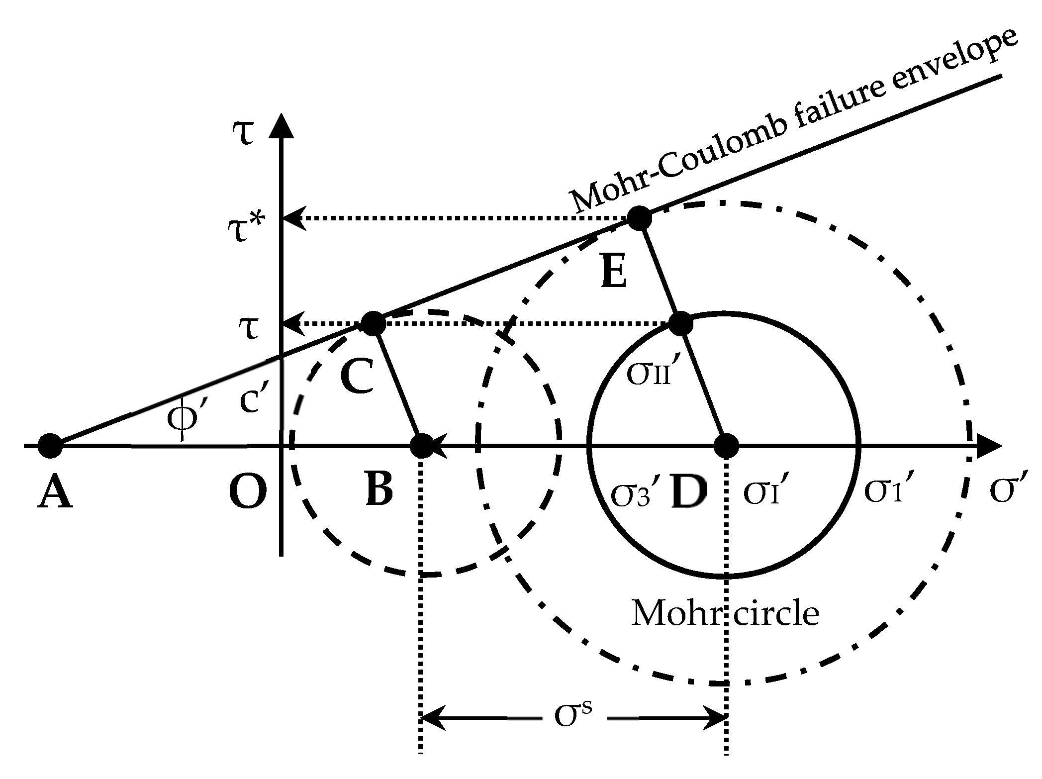
Figure 3.
State of shear stress tensor and the corresponding Mohr circle.
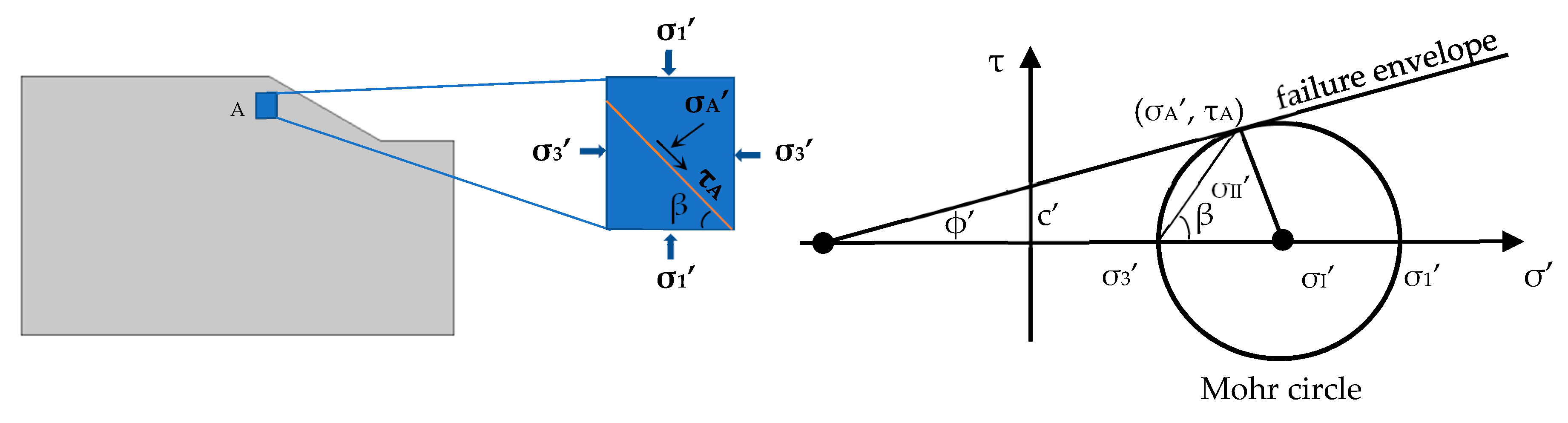
Figure 4.
(a) The geometry, FEM mesh, and boundary conditions of the 2D benchmark model, and (b) the geometry of the 3D benchmark model. The set-up and parameterization of the benchmark model is based on the slope geometry and silty soil used in Lu et al. [30].
Figure 4.
(a) The geometry, FEM mesh, and boundary conditions of the 2D benchmark model, and (b) the geometry of the 3D benchmark model. The set-up and parameterization of the benchmark model is based on the slope geometry and silty soil used in Lu et al. [30].

Figure 5.
The geometry, boundary conditions, and FEM mesh of 2D slopes with two layers of (a) constant layer thickness (Slope A) following Shao et al. (2015) and (b,c) variable layer thickness (Slopes B1 and B2).
Figure 5.
The geometry, boundary conditions, and FEM mesh of 2D slopes with two layers of (a) constant layer thickness (Slope A) following Shao et al. (2015) and (b,c) variable layer thickness (Slopes B1 and B2).

Figure 6.
(a) The surface geometry of the 3D slopes, (b,c), the bedrock topography of the 3D slope C and D, (d) cross-section I through the 3D slope with boundary conditions, and (e) cross-section II through the 3D slope. Arrows are used to indicate dimensions.
Figure 6.
(a) The surface geometry of the 3D slopes, (b,c), the bedrock topography of the 3D slope C and D, (d) cross-section I through the 3D slope with boundary conditions, and (e) cross-section II through the 3D slope. Arrows are used to indicate dimensions.

Figure 7.
The simulated LFS distribution of (a) Lu et al. [30], and our COMSOL implementation in (b) 2D, (c) 3D, and (d) a cross-section through the 3D model.
Figure 7.
The simulated LFS distribution of (a) Lu et al. [30], and our COMSOL implementation in (b) 2D, (c) 3D, and (d) a cross-section through the 3D model.
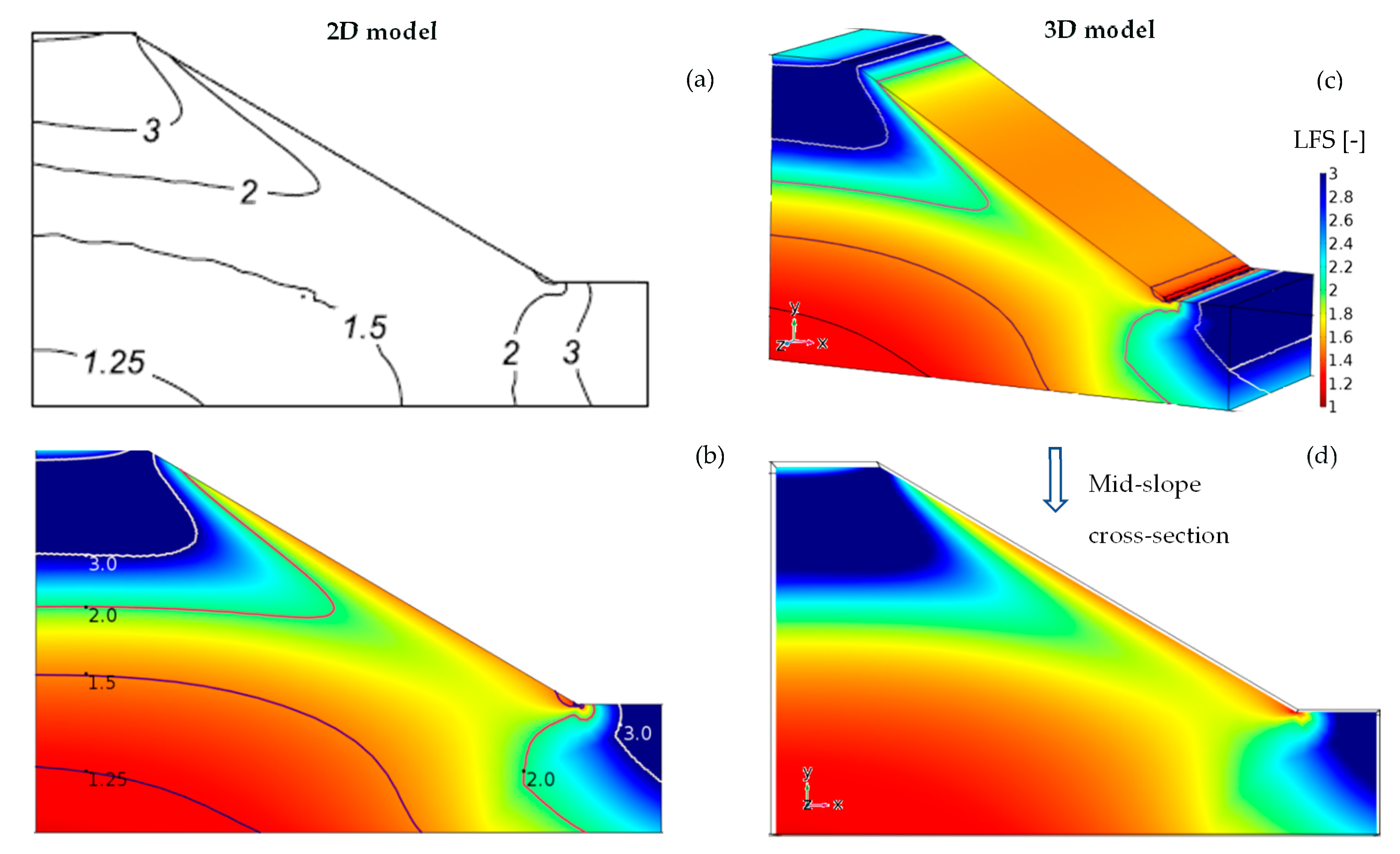
Figure 8.
The temporal development of the soil water content distribution for a 15 h rainfall event with an intensity of 20 mm per hour for the 2D slope with a constant soil depth (slope A) at (a) t = 0 h, (b) t = 7 h, and (c) t = 15 h, and the 2D slopes with variable soil thickness (Slope B1 and B2) at (d,g) t = 0 h, (e,h) t = 7 h, and (f,i) t = 15 h.

Figure 9.
The temporal development of the soil water content distribution for a 150 h rainfall event with an intensity of 2 mm per hour for the 2D slope with a constant soil depth (slope A) at (a) t = 0 h, (b) t = 70 h, and (c) t = 150 h, and the 2D slopes with variable soil thickness (Slope B1 and B2) at (d,g) t = 0 h, (e,h) t = 70 h, and (f,i) t = 150 h.

Figure 10.
(a) Definition of boundaries of the control domain, (b) net infiltration rate into slope A, B1, and B2, (c) outflow at different boundaries of the control area of slope A, (d) outflow at different boundaries of the control area of slope B1, (e) outflow at different boundaries of the control area of slope B2, (f) surface run off of slope A, B1, and B2 as a function of time for the 15-h rainfall event with an intensity of 20 mm per hour.
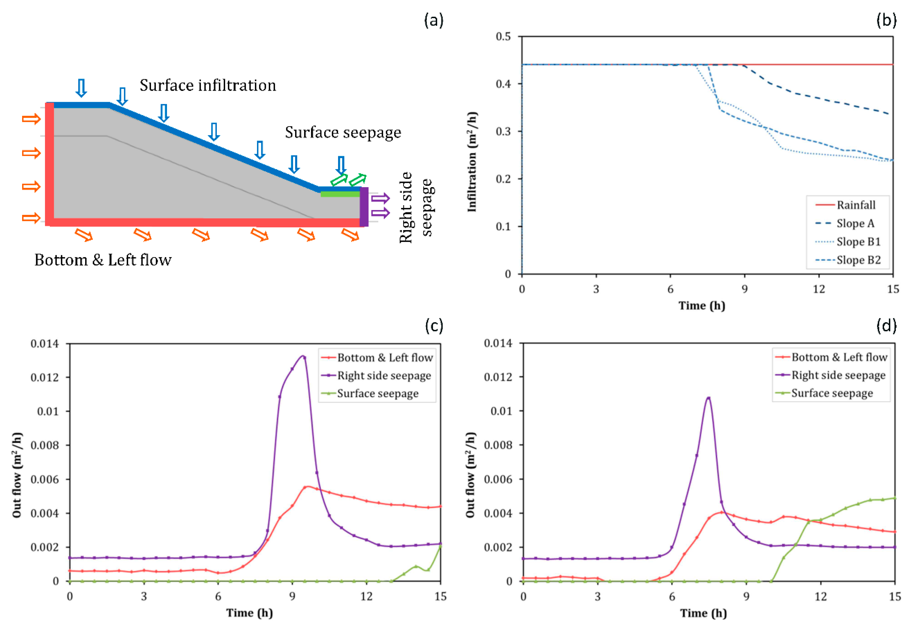

Figure 11.
(a) Definition of boundaries of the control domain, (b) net infiltration rate into slope A, B1, and B2, (c) outflow at different boundaries of the control area of slope A, (d) outflow at different boundaries of the control area of slope B1, (e) outflow at different boundaries of the control area of slope B2, (f) surface run off of slope A, B1, and B2 as a function of time for the 150-h rainfall event with an intensity of 2 mm per hour.

Figure 12.
The temporal development of the LFS distribution for a 15-h rainfall event with an intensity of 20 mm per hour for the 2D slope with a constant soil depth (slope A) at (a) t = 7 h and (b) t = 15 h and the 2D slope with variable soil thickness (Slope B1 and B2) at (c,e) t = 7 h and (d,f) t = 15 h. Black contour lines indicate areas with LFS < 1.0.
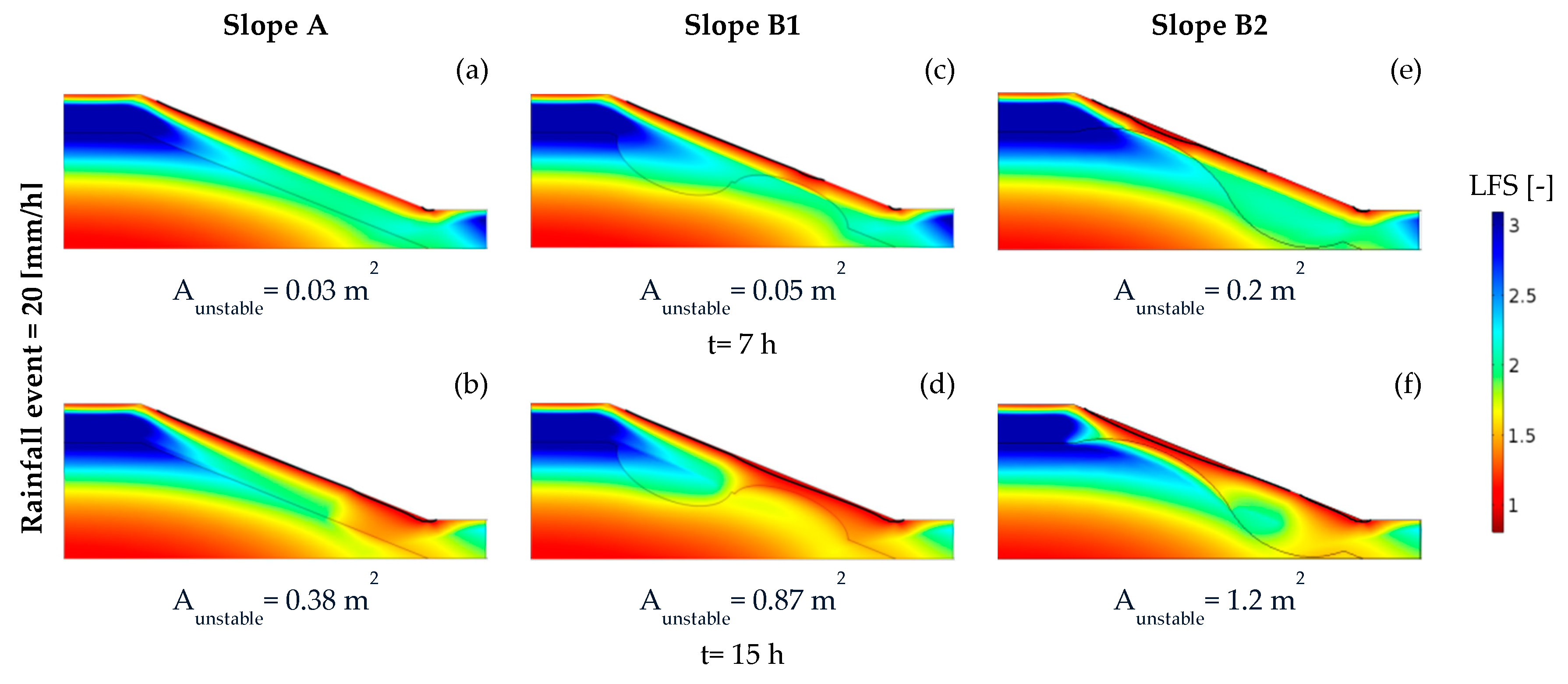
Figure 13.
The temporal development of the LFS distribution for a 150-h rainfall event with an intensity of 2 mm per hour for the 2D slope with a constant soil depth (slope A) at (a) t = 70 h and (b) t = 150 h and the 2D slope with a variable soil thickness (Slope B1 and B2) at (c,e) t = 70 h and (d,f) t = 150 h. Black contour lines indicate areas with LFS < 1.0.
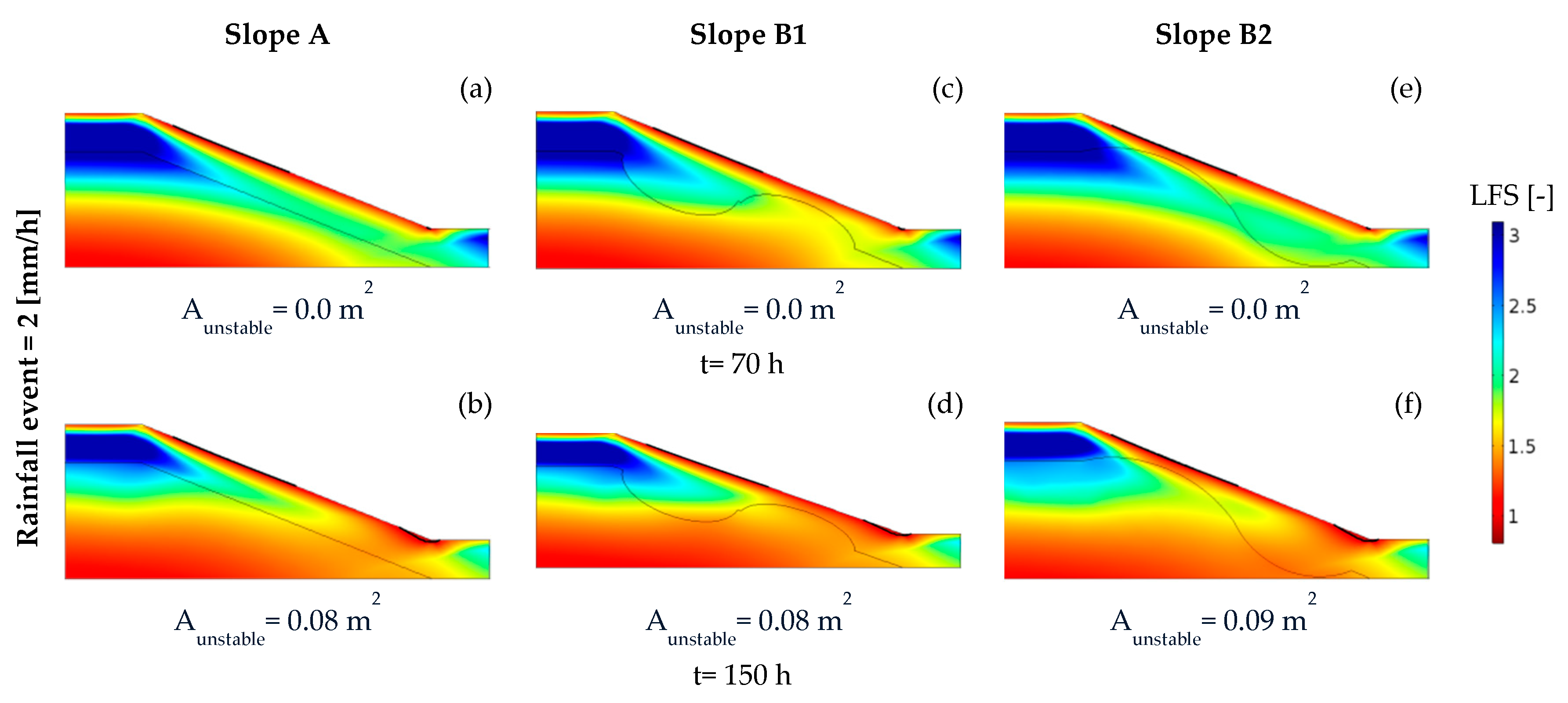
Figure 14.
The temporal development of soil water content of the 2D slope with variable bedrock topography (Slope B1) for (a) t = 0 h, (b) t = 7 h, and (c) t = 15 h, the mid-slope cross-section I of the 3D slope C for (d) t = 0 h, (e) t = 7 h, and (f) t = 15 h and the mid-slope cross-section I of the 3D slope D for (g) t = 0 h, (h) t = 7 h, and (i) t = 15 h after the start of the intensive rainfall event with 20 mm per year.
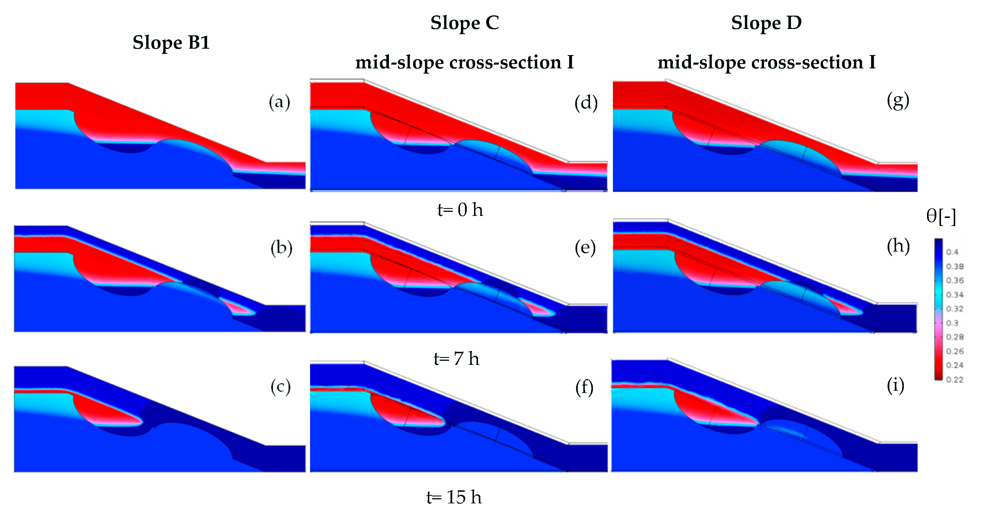
Figure 15.
The temporal development of soil water content for a 15-h rainfall event with an intensity of 20 mm per hour for the 2D slope with a constant soil depth (slope A) at (a) t = 0 h, (b) t = 7 h, and (c) t = 15 h and a cross-section II of slope C, at (d) t = 0 h, (e) t = 7 h, and (f) t = 15 h.
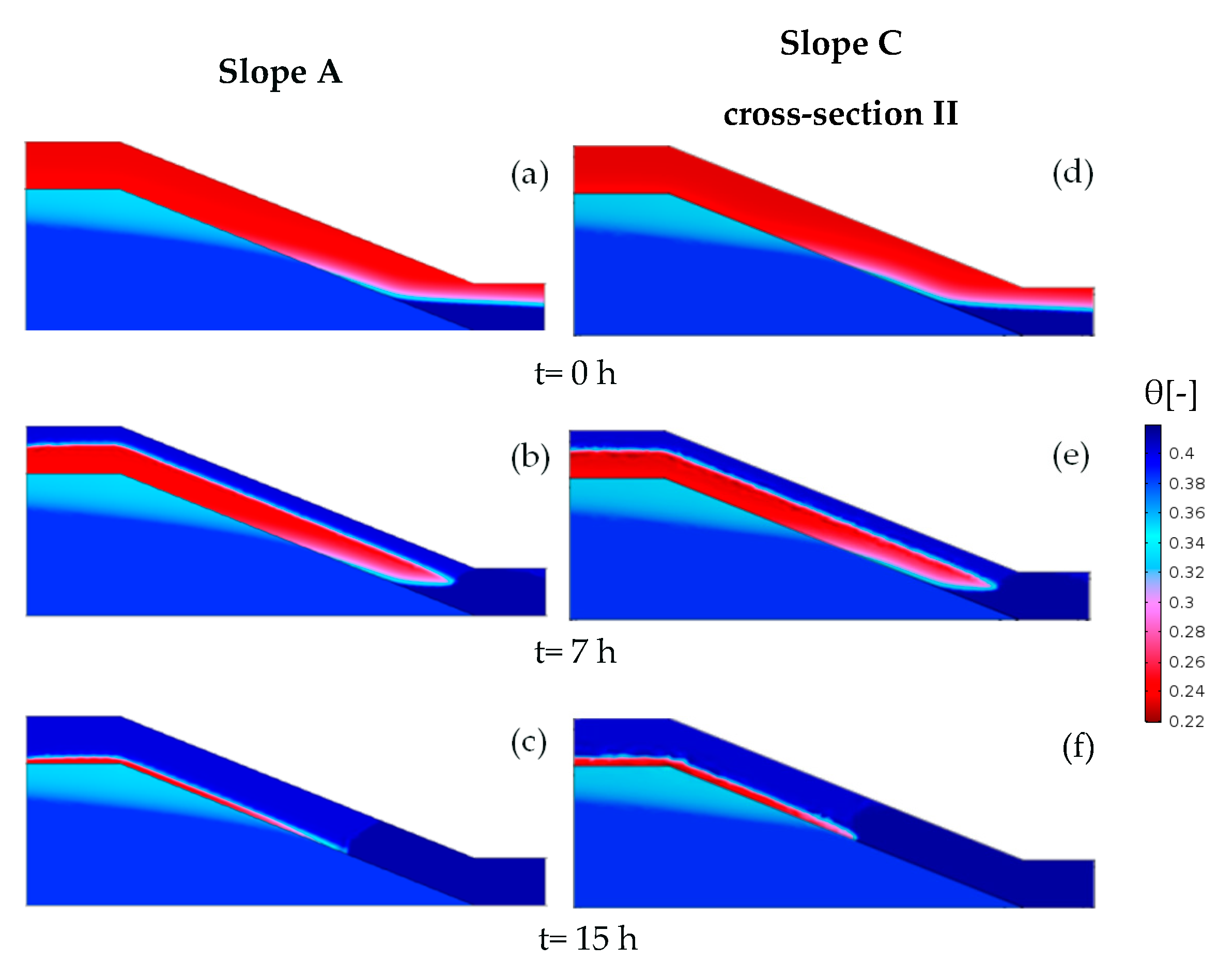
Figure 16.
(a) Definition of boundaries of the control domain, (b) infiltration into 2D slopes B1 and 3D slope D, (c) outflow at different boundaries of the control area of slope B1, and (d) outflow at different boundaries of the control area of slope D as a function of time for the 15-h rainfall event with an intensity of 20 mm per hour.

Figure 17.
The temporal development of the LFS distribution after the start of the intensive rainfall event with 20 mm per hour at t = 7 h and 15 h for (a,b) slope B1 with a variable bedrock topography, (c,d) cross section I of the 3D slope C, and (e,f) cross section I of the 3D slope D.
Figure 17.
The temporal development of the LFS distribution after the start of the intensive rainfall event with 20 mm per hour at t = 7 h and 15 h for (a,b) slope B1 with a variable bedrock topography, (c,d) cross section I of the 3D slope C, and (e,f) cross section I of the 3D slope D.

Figure 18.
The temporal development of the LFS distribution after the start of the intensive rainfall event with 20 mm per hour at t = 7 h and 15 h for (a,b) slope A with a constant soil depth and (c,d) cross-section II of 3D slope C.
Figure 18.
The temporal development of the LFS distribution after the start of the intensive rainfall event with 20 mm per hour at t = 7 h and 15 h for (a,b) slope A with a constant soil depth and (c,d) cross-section II of 3D slope C.


Table 1.
Soil model parameters for the benchmark models.
| Symbol | Parameter Name | Units | Value |
|---|---|---|---|
| Saturated water content | - | 0.46 | |
| Residual water content | - | 0.034 | |
| Ks | Saturated hydraulic conductivity | m s−1 | 1.39 × 10⁻⁶ |
| van Genuchten fitting parameter | m−1 | 1.6 | |
| van Genuchten fitting parameter | - | 1.37 | |
| Dry unit weight | kN m−1 | 20 | |
| E | Young’s modulus | MPa | 10 |
| ν | Poisson’s ratio | - | 0.33 |
| ϕ′ | Friction angle | ° | 30 |
| c′ | Effective cohesion | kPa | 15 |
Table 2.
Soil model parameters for the 2D and 3D numerical experiment (Slope A–D).
| Symbol | Parameter | Units | Value for Top Layer (Sandy Loam) | Value for Bottom Layer (Clay) |
|---|---|---|---|---|
| Saturated water content | - | 0.412 | 0.385 | |
| Residual water content | - | 0.041 | 0.090 | |
| Ks | Saturated hydraulic conductivity | m s−1 | 7.20 × 10⁻⁶ | 1.67 × 10⁻⁷ |
| Brooks-Corey fitting parameter | m−1 | 0.068 | 0.027 | |
| Brooks-Corey fitting parameter | - | 0.322 | 0.131 | |
| Dry unit weight | kN m−1 | 15.5 | 15.5 | |
| E | Young’s modulus | MPa | 10 | 10 |
| ν | Poisson’s ratio | - | 0.35 | 0.35 |
| ϕ′ | Friction angle | ° | 35 | 35 |
| c′ | Effective cohesion | kPa | 5 | 5 |
© 2018 by the authors. Licensee MDPI, Basel, Switzerland. This article is an open access article distributed under the terms and conditions of the Creative Commons Attribution (CC BY) license (http://creativecommons.org/licenses/by/4.0/).
Share and Cite
MDPI and ACS Style
Moradi, S.; Huisman, J.A.; Class, H.; Vereecken, H. The Effect of Bedrock Topography on Timing and Location of Landslide Initiation Using the Local Factor of Safety Concept. Water 2018, 10, 1290. https://doi.org/10.3390/w10101290
AMA Style
Moradi S, Huisman JA, Class H, Vereecken H. The Effect of Bedrock Topography on Timing and Location of Landslide Initiation Using the Local Factor of Safety Concept. Water. 2018; 10(10):1290. https://doi.org/10.3390/w10101290
Chicago/Turabian StyleMoradi, Shirin, Johan Alexander Huisman, Holger Class, and Harry Vereecken. 2018. "The Effect of Bedrock Topography on Timing and Location of Landslide Initiation Using the Local Factor of Safety Concept" Water 10, no. 10: 1290. https://doi.org/10.3390/w10101290
Note that from the first issue of 2016, this journal uses article numbers instead of page numbers. See further details here.