Analysis and Estimation of Geographical and Topographic Influencing Factors for Precipitation Distribution over Complex Terrains: A Case of the Northeast Slope of the Qinghai–Tibet Plateau


Abstract
:1. Introduction
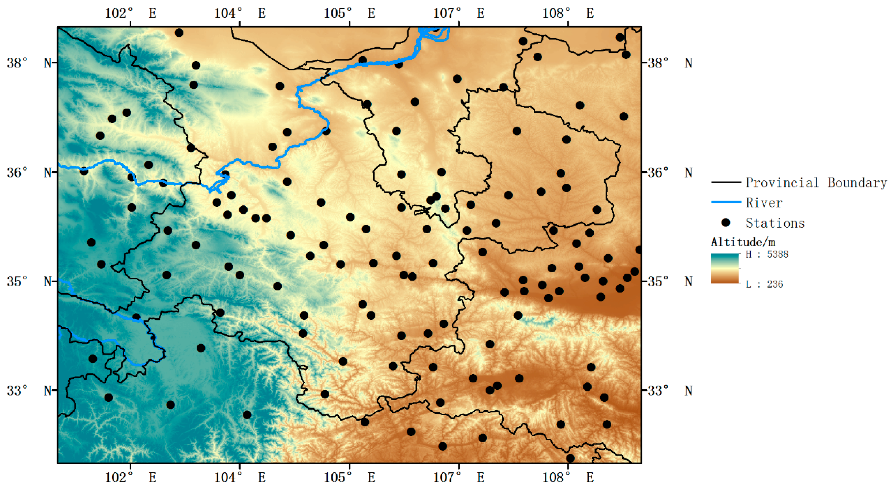
2. Study Area
3. Materials and Methods
3.1. Datasets
3.2. Methods
4. Results
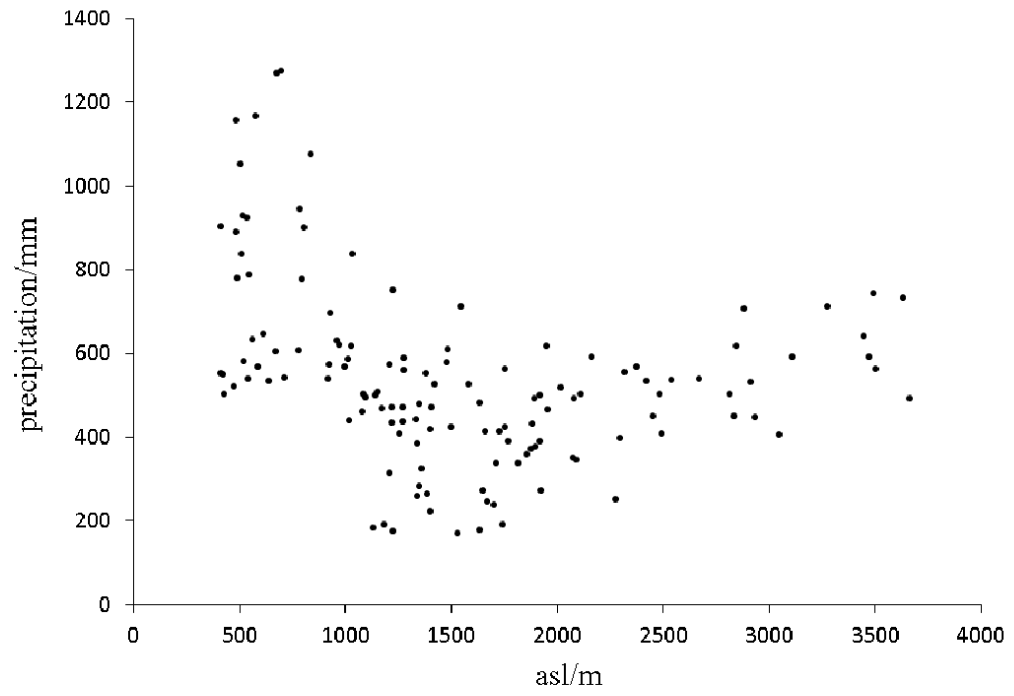
4.1. Precipitation Affecting Factors
4.2. Precipitation Estimating Model
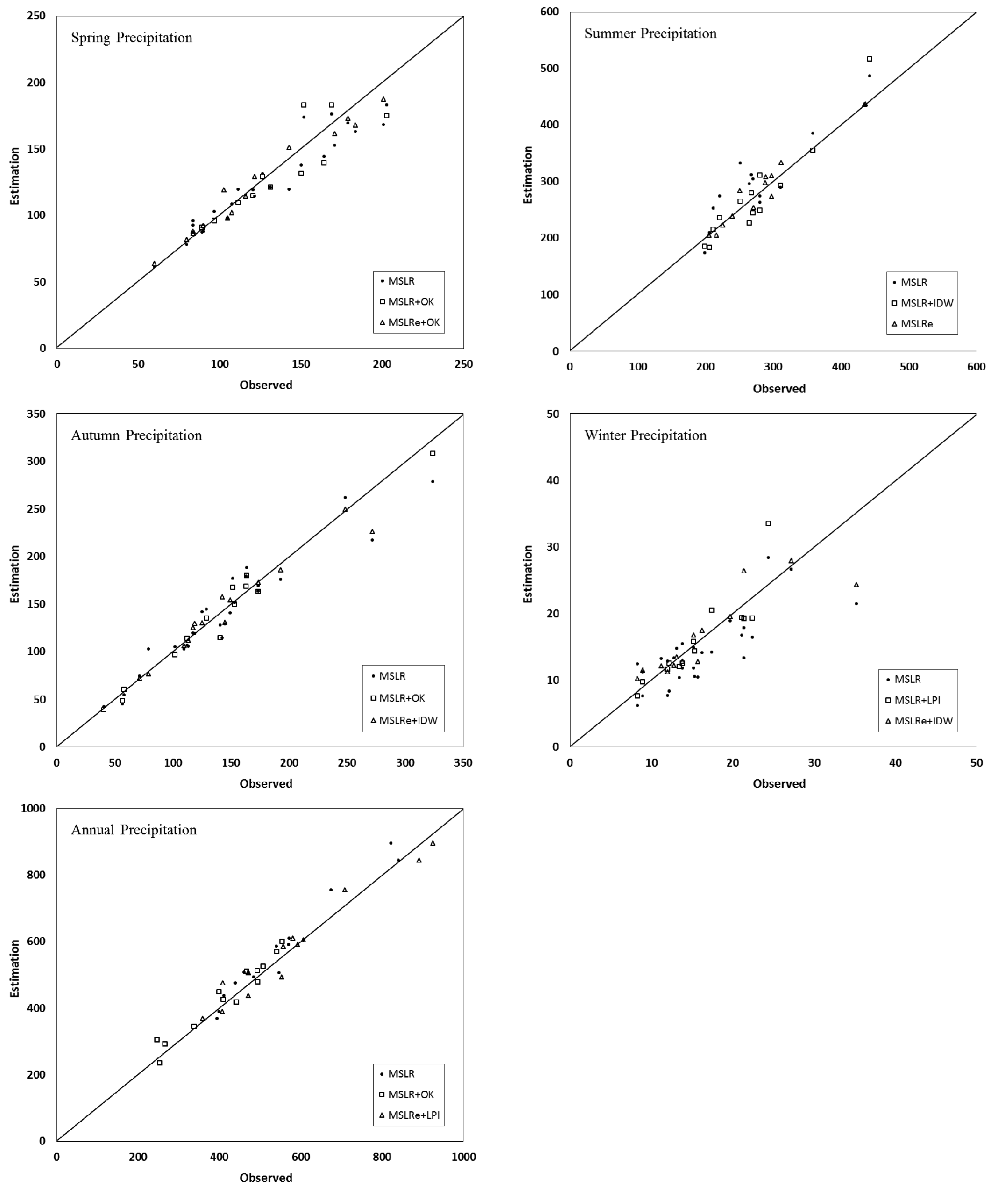
4.3. Precipitation Estimation Verification
5. Discussion
6. Conclusions
Author Contributions
Funding
Conflicts of Interest
References
- Sangati, M.; Borga, M. Influence of rainfall spatial resolution on flash flood modelling. Nat. Hazards Earth Syst. Sci. 2009, 9, 575–584. [Google Scholar] [CrossRef] [Green Version]
- Rana, A.; Uvo, C.B.; Bengtsson, L.; Sarthi, P. Trend analysis for rainfall in Delhi and Mumbai, India. Clim. Dyn. 2012, 38, 45–56. [Google Scholar] [CrossRef]
- Gao, T.; Xie, L. Study on progress of the trends and physical causes of extreme precipitation in China during the last 50 years. Adv. Earth Sci. 2014, 29, 577–589. (In Chinese) [Google Scholar] [CrossRef]
- Wu, G.; Wang, J.; Liu, X.; Liu, Y. Numerical modeling of the influence of eurasian orography on the atmospheric circulation in different seasons. Acta Meteorol. Sin. 2005, 63, 603–612. (In Chinese) [Google Scholar]
- Beniston, M. Mountain weather and climate: A general overview and a focus on climatic change in the Alps. Hydrobiologia 2006, 562, 3–16. [Google Scholar] [CrossRef]
- Zhu, S.; Xu, D.; Xu, M. Structure and Distribution of Rainfall over Mesoscale Mountains in the Asian Summer Monsoon Region. Chin. J. Atmos. Sci. 2010, 34, 71–82. (In Chinese) [Google Scholar]
- Qi, Y.; Fang, S.; Zhou, W. Correlative analysis between the changes of surface solar radiation and its relationship with air pollution, as well as meteorological factor in East and West China in recent 50 years. Acta Phys. Sin. 2015, 64, 089201. (In Chinese) [Google Scholar] [CrossRef]
- Morin, E.; Gabella, M. Radar-based quantitative precipitation estimation over Mediterranean and dry climate regimes. J. Geophys. Res. 2007, 112, 365–371. [Google Scholar] [CrossRef]
- Al-Ahmadi, K.; Al-Ahmadi, S. Spatiotemporal variations in rainfall-topographic relationships in southwestern Saudi Arabia. Arab. J. Geosci. 2014, 7, 3309–3324. [Google Scholar] [CrossRef]
- Saeidabadi, R.; Najafi, M.; Roshan, G.; Fitchett, J.; Abkharabat, S. Modelling spatial, altitudinal and temporal variability of annual precipitation in mountainous regions: The case of the Middle Zagros, Iran. Asia Pac. J. Atmos. Sci. 2016, 52, 437–449. [Google Scholar] [CrossRef]
- Portalés, C.; Boronat, N.; Pardo-Pascual, J.; Balaguer-Beser, A. Seasonal precipitation interpolation at the Valencia region with multivariate methods using geographic and topographic information. Int. J. Clim. 2010, 30, 1547–1563. [Google Scholar] [CrossRef]
- Marquinez, J.; Lastra, J.; Garcia, P. Estimation models for precipitation in mountainous regions: The use of GIS and multivariate analysis. J. Hydrol. 2003, 270, 1–11. [Google Scholar] [CrossRef]
- Shu, S.; Wang, Y.; Xiong, A. Estimation and analysis for geographic and orographic influences on precipitation distribution in China. Chin. J. Geophys. 2007, 50, 1703–1712. (In Chinese) [Google Scholar] [CrossRef]
- Shu, S.; Yu, Z.; Wang, Y.; Bai, M. A statistic model for the spatial distribution of precipitation estimation over the Tibetan complex terrain. Chin. J. Geophys. 2005, 48, 535–542. (In Chinese) [Google Scholar] [CrossRef]
- Zhao, C.; Feng, Z.; Nan, Z. Modelling the Temporal and Spatial Variabil ities of Precipitation in Zulihe River Basin of the Western Loess Plateau. Plateau Meteorol. 2008, 27, 208–214. (In Chinese) [Google Scholar]
- Du, L.; Li, J.; Chen, X.; Shang, K.; Yang, D.; Wang, S. Analysis on Cloud and Vapor Flux in the Northeast of the Qinghai-Tibet Plateau during the Period from 2001 to 2011. Arid Zone Res. 2012, 29, 862–869. (In Chinese) [Google Scholar]
- Zhang, J.; Li, D.; He, J.; Wang, X. Influence of terrain on precipitation distribution in Qingzang tableland in wet and dry years. Adv. Water Sci. 2007, 18, 319–326. [Google Scholar]
- Wei, H.; Li, J.; Liang, T. Study on the esitmation of precipitation resources for rainwater harvesting agriculture in semi-arid land of China. Agric. Water Manag. 2005, 71, 33–45. [Google Scholar] [CrossRef]
- Peng, S.; Zhao, C.; Wang, X.; Xu, Z.; Liu, X.; Hao, H.; Yang, S. Mapping Daily Temperature and Precipitation in the Qilian Mountains of Northwest China. J. Mt. Sci. 2014, 11, 896–905. [Google Scholar] [CrossRef]
- Yu, Y.; Wei, W.; Chen, L.; Yang, L.; Zhang, H. Comparison on the methods for spatial interpolation of the annual average precipitation in the Loess Plateau region. Chin. J. Appl. Ecol. 2015, 26, 999–1006. (In Chinese) [Google Scholar]
- National Meteorological Information Center. Standard Monthly Dataset of Chinese Surface Climate. Available online: http://data.cma.cn (accessed on 5 August 2017).
- Ren, Z.; Xiong, A.; Zou, F. The Quality Control of Surface Monthly Climate Data in China. J. Appl. Meteorol. Sci. 2007, 18, 516–523. (In Chinese) [Google Scholar]
- Liu, W.; Zhang, Q.; Fu, Z. Variation Characteristics of Precipitation and Its Affecting Factors in Northwest China over the Past 55 Years. Plateau Meteorol. 2017, 36, 1533–1545. (In Chinese) [Google Scholar] [CrossRef]
- National Aeronautics and Space Administration (NASA) and National Geospatial-Intelligence Agency (NGA). SRTM Data Set. Available online: http://srtm.csi.cgiar.org/index.asp (accessed on 14 October 2017).
- Donges, J.F.; Petrova, I.; Loew, A.; Marwan, N.; Kurths, J. How complex climate networks complement eigen techniques for the statistical analysis of climatological data. Clim. Dyn. 2013, 45, 2407–2424. [Google Scholar] [CrossRef]
- Diaconescu, E.P.; Gachon, P.; Scinocca, P.; Laprise, R. Evaluation of daily precipitation statistics and monsoon onset/retreat over western Sahel in multiple data sets. Clim. Dyn. 2014, 45, 1325–1354. [Google Scholar] [CrossRef] [Green Version]
- Draper, N.R.; Smith, H. Applied Regression Analysis, 3rd ed.; Wiley: New York, NY, USA, 1998. [Google Scholar]
- Kohavi, R. A study of cross-validation and bootstrap for accuracy estimation and model selection. In Proceedings of the Fourteenth International Joint Conference on Artificial Intelligence, Montreal, QC, Canada, 20–25 August 1995; Morgan Kaufmann: San Mateo, CA, USA, 1995; pp. 1137–1143. [Google Scholar]
- Hastie, T.; Tibshirani, R.; Friedman, J.H. The Elements of Statistical Learning: Data Mining Inference and Prediction; Springer: New York, NY, USA, 2001. [Google Scholar]
- Bartier, P.M.; Keller, C.P. Multivariate interpolation to incorporate thematic surface data using inverse distance weighting. Comput. Geosci. 1996, 22, 795–799. [Google Scholar] [CrossRef]
- Daly, C. Guidelines for assessing the suitability of spatial climate data sets. Int. J. Clim. 2006, 26, 707–721. [Google Scholar] [CrossRef] [Green Version]
- Fatichi, S.; Caporali, E. A comprehensive analysis of changes in precipitation regime in Tuscany. Int. J. Clim. 2009, 29, 1883–1893. [Google Scholar] [CrossRef] [Green Version]
- Francisco, M.; Vilar, J.M. Local polynomial regression estimation with correlated errors. Commun. Stat. 2001, 30, 1271–1293. [Google Scholar] [CrossRef]
- Williams, C.K.I. Prediction with Gaussian Processes: From Linear Regression to Linear Prediction and Beyond; Springer: Dordrecht, The Netherlands, 1989. [Google Scholar]
- Morlier, J.; Chermain, B.; Gourinat, Y. Original statistical approach for the reliability in modal parameters estimation. J. Hazard. Mater. 2009, 114, 240–248. [Google Scholar]
- Hyndman, R.J.; Koehler, A.B. Another look at measures of forecast accuracy. Int. J. Forecast. 2006, 22, 679–688. [Google Scholar] [CrossRef] [Green Version]
- Harris, G.N.; Bowman, K.P.; Shin, D.B. Comparison of freezing-level altitudes from the NCEP reanalysis with TRMM precipitation radar brightband data. J. Clim. 2000, 13, 4137–4148. [Google Scholar] [CrossRef]
- Zhao, A.; Zhang, M.; Sun, M.; Wang, B.; Wang, S.; Wang, Q. Changes in 0 °C isotherm height of Southwest China during 1960–2010. Acta Geogr. Sin. 2013, 68, 994–1006. (In Chinese) [Google Scholar]
- Chen, Z.; Chen, Y.; Li, W. Response of runoff to change of atmospheric 0 °C level height in summer in arid region of Northwest China. Sci. China Earth Sci. 2012, 55, 1533–1544. [Google Scholar] [CrossRef]
- Chen, T.Y.; Li, Z.R.; Chen, Q.; Li, B.Z. The Analysis of Climate Characteristics of Water Vapor Distribution over Northwest China with Water Vapor Field Retrieved from GMS5 Satellite Data. Chin. J. Atmos. Sci. 2005, 29, 864–871. [Google Scholar]
- Wang, X.; Xu, X.; Wang, W. Charateristic of Spatial Transportation of Water Vapor for Northwest China’s Rainfall in Spring and Summer. Plateau Meteorol. 2007, 26, 749–758. (In Chinese) [Google Scholar]
- Zhang, Z.; Zhang, Q.; Zhao, Q.; Zhang, L.; Cai, Y. Radar quantitative precipitation inversion and its application to areal rainfall estimation in the northeastern marginal areas of the Tibetan Plateau. J. Glaciol. Geocryol. 2013, 35, 621–629. (In Chinese) [Google Scholar] [CrossRef]
- Xu, X.; Du, Y.G.; Tang, J.P.; Wang, Y. Variations of temperature and precipitation extremes in recent two decades over China. Atmos. Res. 2011, 101, 143–154. [Google Scholar] [CrossRef]
- Mizukami, N.; Smith, M.B. Analysis of inconsistencies in multi-year gridded quantitative precipitation estimate over complex terrain and its impact on hydrologic modeling. J. Hydrol. 2012, 428–429, 129–141. [Google Scholar] [CrossRef]
- Delbari, M.; Afrasiab, P.; Jahani, S. Spatial interpolation of monthly and annual rainfall in northeast of Iran. Meteorol. Atmos. Phys. 2013, 122, 103–113. [Google Scholar] [CrossRef]
- Gou, Y.; Ma, Y.; Chen, H.; Wen, Y. Radar-derived quantitative precipitation estimation in complex terrain over the eastern Tibetan Plateau. Atmos. Res. 2018, 203, 286–297. [Google Scholar] [CrossRef]
- Henn, B.; Newman, A.J.; Livneh, B.; Daly, C.; Lundquist, J.D. An assessment of differences in gridded precipitation datasets in complex terrain. J. Hydrol. 2018, 556, 1205–1209. [Google Scholar] [CrossRef]
- Colle, B.A.; Mass, C.F.; Westrick, K.J. Mesoscale modeling of precipitation in complex orography along the west coast of North America. In Proceedings of the 8th Conference on Moutain Meteorology, Flagstaff, AZ, USA, 3–7 August 1998. [Google Scholar]
- Junquas, C.; Li, L.; Vera, C.S.; Treut, H.L.; Takahashi, K. Influence of South America orography on summertime precipitation in Southeastern South America. Clim. Dyn. 2016, 46, 3941–3963. [Google Scholar] [CrossRef]
- Fortin, V.; Roy, G.; Donaldson, N.; Mahidjiba, A. Assimilation of radar quantitative precipitation estimations in the Canadian Precipitation Analysis (CaPA). J. Hydrol. 2015, 531, 296–307. [Google Scholar] [CrossRef]
- Rafieeinasab, A.; Norouzi, A.; Seo, D.-J.; Nelson, B. Improving high-resolution quantitative precipitation estimation via fusion of multiple radar-based precipitation products. J. Hydrol. 2015, 531, 320–336. [Google Scholar] [CrossRef]
- Zhao, H.; Yang, B.; Yang, S.; Huang, Y.; Dong, G.; Bai, J.; Wang, Z. Systematical estimation of GPM-based global satellite mapping of precipitation products over China. Atmos. Res. 2018, 201, 206–217. [Google Scholar] [CrossRef]


| Parameters | Units | Resolution |
|---|---|---|
| Latitude (Lat) | Degrees | 0.001° |
| Longitude (Lon) | Degrees | 0.001° |
| Altitude (Alt) | Meters | 250 m |
| Mean altitude within a 5-km radius (Malt) | Meters | 250 m |
| Mean slope within a 5-km radius (Ms) | Degrees | 1° |
| Mean aspect within a 10-km radius (Masp) | Degrees | 1° |
| Tangent of the average aspect within a 10-km radius (Tm) | - | 0.01 |
| Maximum altitude of the eastern sector within a 50-km radius (MaE) | Meters | 250 m |
| Maximum altitude of the southern sector within a 50-km radius (MaS) | Meters | 250 m |
| Maximum altitude of the western sector within a 50-km radius (MaW) | Meters | 250 m |
| Maximum altitude of the northern sector within a 50-km radius (MaN) | Meters | 250 m |
| Parameters | Spring | Summer | Autumn | Winter | Annual |
|---|---|---|---|---|---|
| Lat | −0.88 ** | −0.79 ** | −0.86 ** | −0.72 ** | −0.84 ** |
| Lon | 0.17 | 0.24 ** | 0.37 ** | 0.45 ** | 0.28 ** |
| Alt | −0.19 * | −0.24 * | −0.38 ** | −0.38 ** | −0.28 ** |
| Malt | −0.06 | −0.12 | −0.22 * | −0.31 ** | −0.15 |
| Ms | 0.37 ** | 0.31 ** | 0.32 ** | 0.28 ** | 0.33 ** |
| Tm | 0.19 | 0.18 | 0.17 | 0.16 | 0.18 |
| MaE | 0.11 | 0.01 | −0.09 | −0.25 ** | −0.01 |
| MaS | 0.06 | −0.04 | −0.14 | −0.26 ** | −0.06 |
| MaW | 0.16 | 0.10 | −0.02 | −0.16 | 0.07 |
| MaN | 0.12 | 0.05 | −0.06 | −0.21 * | 0.02 |
| Parameters | Spring | Summer | Autumn | Winter | Annual |
|---|---|---|---|---|---|
| Lat | −0.89 ** | −0.81 ** | −0.87 ** | −0.74 ** | −0.85 ** |
| Lon | 0.30 * | 0.28 * | 0.38 ** | 0.43 ** | 0.32 ** |
| Alt | −0.65 ** | −0.56 ** | −0.70 ** | −0.65 ** | −0.63 ** |
| Malt | −0.22 | −0.23 | −0.31 * | −0.36 ** | −0.26 * |
| Ms | 0.50 ** | 0.47 ** | 0.53 ** | 0.59 ** | 0.51 ** |
| Tm | 0.18 | 0.15 | 0.18 | 0.18 | 0.17 |
| MaE | 0.20 | 0.16 | 0.10 | −0.10 | 0.14 |
| MaS | 0.07 | 0.02 | −0.03 | −0.16 | 0.01 |
| MaW | 0.34 ** | 0.33 ** | 0.25 * | 0.08 | 0.30 * |
| MaN | 0.21 | 0.21 | 0.14 | −0.04 | 0.19 |
| Parameters | Spring | Summer | Autumn | Winter | Annual |
|---|---|---|---|---|---|
| Lat | −0.84 ** | −0.71 ** | −0.87 ** | −0.65 ** | −0.82 ** |
| Lon | −0.24 | −0.21 | −0.22 | 0.18 | −0.21 |
| Alt | 0.52 ** | 0.72 ** | 0.68 ** | 0.47 ** | 0.68 ** |
| Malt | 0.34 * | 0.44 ** | −0.44 ** | 0.11 | 0.42 ** |
| Ms | 0.22 | 0.10 | −0.13 | −0.12 | 0.14 |
| Tm | 0.28 | 0.42 * | −0.31 | 0.26 | 0.37 * |
| MaE | 0.31 | 0.25 | 0.33 * | −0.05 | 0.28 |
| MaS | 0.39 * | 0.35 * | 0.40 * | 0.03 | 0.38 * |
| MaW | 0.26 | 0.30 | 0.33 * | −0.03 | 0.30 |
| MaN | 0.31 | 0.27 | 0.32 | −0.04 | 0.30 |
| Parameter | Spring | Summer | Autumn | Winter | Annual |
|---|---|---|---|---|---|
| (a) Coefficients βn | |||||
| Lat | −23.697 | −54.290 | −32.320 | −3.822 | −115.069 |
| Lon | 7.230 | 23.157 | 15.087 | 1.762 | 50.916 |
| Alt | 0.013 | 0.038 | 0.012 | 0.002 | 0.065 |
| Malt | −0.031 | −0.094 | −0.042 | −0.176 | |
| Ms | 0.983 | ||||
| Tm | 0.613 | ||||
| MaE | 0.010 | 0.010 | 0.003 | 0.026 | |
| MaS | −0.001 | ||||
| MaW | 0.018 | 0.065 | 0.029 | 0.107 | |
| MaN | 0.018 | −0.005 | 0.032 | ||
| (b) Intercept β0 | |||||
| 142.634 | −344.938 | −371.816 | −40.669 | −982.122 | |
| (c) Adjusted coefficient of determination | |||||
| 0.81 | 0.70 | 0.84 | 0.71 | 0.79 | |
| Parameters | Spring | Summer | Autumn | Winter | Annual | Parameters | Spring | Summer | Autumn | Winter | Annual |
|---|---|---|---|---|---|---|---|---|---|---|---|
| (EMB) | (EMA) | ||||||||||
| (a) Coefficients βn | (a) Coefficients βn | ||||||||||
| Lat | −24.655 | −60.277 | −35.136 | −3.487 | −123.561 | Lat | −19.322 | −24.849 | −18.74 | −1.497 | −63.504 |
| Lon | 11.059 | 25.36 | 15.931 | 1.57 | 53.599 | Lon | 1.464 | ||||
| Alt | 0.020 | 0.083 | 0.018 | 0.003 | 0.110 | Alt | 0.012 | 0.063 | 0.025 | 0.006 | 0.099 |
| Malt | −0.04 | −0.164 | −0.069 | −0.007 | −0.237 | Malt | −0.007 | ||||
| Ms | Ms | ||||||||||
| Tm | 0.343 | Tm | |||||||||
| MaE | 0.022 | 0.010 | 0.108 | MaE | −0.024 | −0.010 | −0.037 | −0.024 | |||
| MaS | −0.010 | −0.082 | MaS | ||||||||
| MaW | 0.022 | 0.066 | 0.015 | 0.002 | 0.139 | MaW | |||||
| MaN | 0.056 | 0.023 | MaN | −0.002 | |||||||
| (b) Intercept β0 | (b) Intercept β0 | ||||||||||
| −241.158 | −394.242 | −337.254 | −30.707 | −939.533 | 771.326 | 1066.042 | 747.08 | −95.496 | |||
| (c) Adjusted Coefficient of Determination | (c) Adjusted Coefficient of Determination | ||||||||||
| 0.90 | 0.76 | 0.89 | 0.72 | 0.85 | 0.73 | 0.76 | 0.79 | 0.75 | 0.81 | ||
| (a) | (b) | ||||||||
|---|---|---|---|---|---|---|---|---|---|
| Methods | R | ME/% | MAE/% | RMSE/% | Methods | R | ME/% | MAE/% | RMSE/% |
| Spring | Spring | ||||||||
| MSLR | 0.93 | −0.30 | 8.79 | 10.36 | MSLR | 0.97 | −0.13 | 7.08 | 8.72 |
| MSLR + IDW | 0.92 | −0.30 | 9.44 | 10.92 | MSLR + IDW | 0.87 | 0.40 | 11.67 | 17.19 |
| MSLR + LPI | 0.91 | −0.30 | 8.59 | 11.15 | MSLR + LPI | 0.92 | 0.58 | 10.34 | 13.35 |
| MSLR + OK | 0.93 | −0.03 | 8.29 | 10.23 | MSLR + OK | 0.98 | 0.15 | 5.70 | 6.66 |
| Summer | Summer | ||||||||
| MSLR | 0.91 | 0.86 | 12.69 | 15.29 | MSLR | 0.89 | −0.04 | 8.57 | 11.71 |
| MSLR + IDW | 0.96 | −0.08 | 8.10 | 9.24 | MSLR + IDW | 0.77 | 0.17 | 12.04 | 14.30 |
| MSLR + LPI | 0.93 | 0.02 | 9.60 | 10.88 | MSLR + LPI | 0.80 | 0.81 | 11.88 | 17.78 |
| MSLR + OK | 0.94 | 0.02 | 8.67 | 9.73 | MSLR + OK | 0.82 | 0.58 | 11.64 | 14.90 |
| Autumn | Autumn | ||||||||
| MSLR | 0.97 | 0.05 | 9.32 | 10.86 | MSLR | 0.94 | −0.16 | 9.65 | 12.62 |
| MSLR + IDW | 0.99 | 0.08 | 8.62 | 10.01 | MSLR + IDW | 0.97 | 0.06 | 5.17 | 6.91 |
| MSLR + LPI | 0.99 | −0.28 | 7.21 | 8.77 | MSLR + LPI | 0.97 | 0.14 | 6.18 | 9.55 |
| MSLR +OK | 0.99 | −0.12 | 6.81 | 8.28 | MSLR + OK | 0.92 | 0.28 | 10.29 | 13.48 |
| Winter | Winter | ||||||||
| MSLR | 0.84 | −1.94 | 23.90 | 25.09 | MSLR | 0.84 | −0.01 | 17.36 | 22.50 |
| MSLR + IDW | 0.84 | 0.32 | 14.75 | 18.97 | MSLR + IDW | 0.87 | 0.32 | 12.67 | 16.15 |
| MSLR + LPI | 0.89 | 0.06 | 10.64 | 13.76 | MSLR + LPI | 0.86 | 0.48 | 16.40 | 21.03 |
| MSLR + OK | 0.86 | 0.10 | 11.04 | 15.34 | MSLR + OK | 0.86 | 0.07 | 18.13 | 22.42 |
| Annual | Annual | ||||||||
| MSLR | 0.90 | 0.36 | 12.15 | 14.08 | MSLR | 0.97 | −0.18 | 6.64 | 8.24 |
| MSLR + IDW | 0.88 | 0.91 | 14.32 | 19.77 | MSLR + IDW | 0.89 | 0.04 | 10.29 | 12.23 |
| MSLR + LPI | 0.89 | 1.13 | 12.79 | 18.90 | MSLR + LPI | 0.98 | 0.02 | 5.88 | 7.19 |
| MSLR + OK | 0.97 | 0.54 | 7.73 | 9.61 | MSLR + OK | 0.86 | 0.05 | 11.71 | 15.63 |
© 2018 by the authors. Licensee MDPI, Basel, Switzerland. This article is an open access article distributed under the terms and conditions of the Creative Commons Attribution (CC BY) license (http://creativecommons.org/licenses/by/4.0/).
Share and Cite
Liu, W.; Zhang, Q.; Fu, Z.; Chen, X.; Li, H. Analysis and Estimation of Geographical and Topographic Influencing Factors for Precipitation Distribution over Complex Terrains: A Case of the Northeast Slope of the Qinghai–Tibet Plateau. Atmosphere 2018, 9, 349. https://doi.org/10.3390/atmos9090349
Liu W, Zhang Q, Fu Z, Chen X, Li H. Analysis and Estimation of Geographical and Topographic Influencing Factors for Precipitation Distribution over Complex Terrains: A Case of the Northeast Slope of the Qinghai–Tibet Plateau. Atmosphere. 2018; 9(9):349. https://doi.org/10.3390/atmos9090349
Chicago/Turabian StyleLiu, Weicheng, Qiang Zhang, Zhao Fu, Xiaoyan Chen, and Hong Li. 2018. "Analysis and Estimation of Geographical and Topographic Influencing Factors for Precipitation Distribution over Complex Terrains: A Case of the Northeast Slope of the Qinghai–Tibet Plateau" Atmosphere 9, no. 9: 349. https://doi.org/10.3390/atmos9090349