


Abstract
Urban air pollution remains a major challenge in rapidly growing metropolitan regions, but pollutant behavior and meteorological controls differ substantially among cities. This study compares air-quality trends in Shanghai, Delhi, Paris, Los Angeles, and São Paulo during 2018–2023 using observations of PM2.5, PM10, O3, NO2, and SO2 together with temperature, sea-level pressure, and wind speed. Annual and seasonal means, exceedance frequencies, and pollutant–meteorology relationships were evaluated. PM2.5 declined in Shanghai from 43.52 µg/m3 in 2018 to 27.02 µg/m3 in 2022 before increasing to 30.28 µg/m3 in 2023. Delhi remained the most persistently polluted city, with PM2.5 remaining above 87 µg/m3 throughout the period, whereas Los Angeles maintained substantially lower PM2.5 concentrations. Paris showed declining PM2.5 and NO2, while São Paulo exhibited increasing PM2.5 by 2023. The analysis of the study concerning exceedances showed that Delhi and Shanghai had 2025 and 1881 PM2.5 exceedance days, respectively, as compared to 366 in Los Angeles. For O3, Los Angeles had the highest number of exceedance days, 1973, followed by Shanghai, 1801, then Paris, 1347, and São Paulo, 1196, whereas Delhi had the lowest figure, 571. Moreover, when the influence of meteorological factors on PM2.5 and O3 is examined, it is observed that temperature was negatively correlated with PM2.5 in Delhi (r = −0.66), in Shanghai (r = −0.25), and in Paris (r = −0.21), while Los Angeles (r = 0.16) and São Paulo (r = 0.09) showed a weak positive relationship. Sea-level pressure was most strongly associated with PM2.5 in Delhi (r = 0.65), and wind speed was negatively correlated with PM2.5 in all five cities. Temperature–ozone relationships were strongest in Paris (r = 0.71) and Los Angeles (r = 0.66). These results emphasize strong city-specific differences in pollutant trends and meteorological sensitivity and support locally tailored air-quality management strategies.
1. Introduction
Air pollution in megacities is shaped by the interaction of dense populations, transportation, industrial activity, energy use, atmospheric chemistry, and meteorology. Fine particulate matter with aerodynamic diameters ≤ 2.5 µm (PM2.5) and ≤10 µm (PM10), ozone (O3), nitrogen dioxide (NO2), and sulfur dioxide (SO2) remain important indicators of urban air quality because of their documented effects on human health and ecosystems [1,2,3,4]. Urban growth, changes in energy use and transportation, and the continued expansion of metropolitan regions can alter both emissions and local atmospheric processes.
Megacities are particularly important for air-quality research because large emissions and dense populations produce substantial exposure, while their atmospheric influence can extend beyond municipal boundaries through regional transport. Their complex-built environments, land-use patterns, and urban heat-island effects can also modify circulation, atmospheric mixing, and pollutant dispersion [5,6].
Previous work has shown that global urban PM2.5 and NO2 trends vary strongly by region, while O3 exposure has increased in many urban areas [2,7]. These trends also differ by pollutant. PM2.5 and NO2 may respond comparatively directly to controls on combustion and transportation emissions, whereas O3 is formed through nonlinear photochemical reactions involving nitrogen oxides and volatile organic compounds. Consequently, reductions in primary pollutants or individual ozone precursors do not necessarily produce corresponding reductions in ambient O3. Megacities are especially useful for comparative analysis because they combine high emissions with distinctive topography, climate, transportation systems, regulatory histories, and regional pollution transport [5,8,9]. The COVID-19 period introduced an unusual disruption in transportation, industrial activity, and other anthropogenic emissions: restrictions on transportation and industrial activity reduced several primary pollutants in many locations, while O3 responses were often more complex because of nonlinear photochemistry and reduced NO titration [10,11,12]. O3 responses were more heterogeneous because of nonlinear precursor chemistry, changes in NO titration, and meteorological variability [10,11,12]. The period therefore requires cautious interpretation rather than direct attribution of all 2020 changes to lockdown restrictions.
Meteorological conditions strongly influence pollutant accumulation and removal. Low wind speeds, high-pressure stagnation, shallow boundary layers, and winter inversions can increase particulate concentrations, whereas stronger winds, precipitation, and enhanced vertical mixing can reduce near-surface PM2.5 [13,14,15]. Ozone generally responds differently because photochemical production is enhanced by sunlight and temperature, although the magnitude and even strength of this relationship depend on precursor emissions and chemical regime. The direction and strength of pollutant–meteorology relationships can therefore differ among cities because of variations in topography, emissions, atmospheric chemistry, seasonal circulation, and regional transport. Moreover, individual meteorological variables frequently covary with one another and with seasonal emissions. Statistical correlations should consequently be interpreted as indicators of association rather than direct evidence of causality.
Although numerous studies have examined air pollution within individual megacities, direct comparisons across cities remain difficult because of differences in monitoring systems, pollutant sources, climatic regimes, seasonal cycles, urban form, and regulatory history. Global trend studies provide broad geographical coverage but may not capture the combination of annual trends, seasonal behavior, threshold exceedances, and pollutant–meteorology relationships within individual urban environments. Conversely, city-specific studies provide greater local details but do not always show how the observed relationships compare across contrasting megacities. A common comparative framework can help identify which features are broadly shared and which are strongly dependent on local emissions and meteorology.
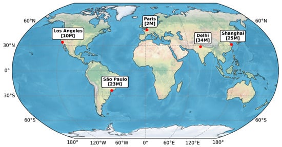
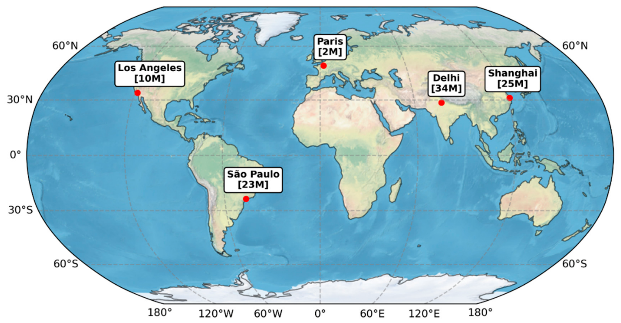
This study compares five megacities—Shanghai, Delhi, Paris, Los Angeles, and São Paulo—chosen to span different climatic regions, pollutant emissions profiles, policy environments, and stages of air-quality management (Figure 1). Shanghai and Delhi represent densely populated Asian megacities with substantial particulate pollution but different coastal, continental, and seasonal influences. Paris represents a European city with strong transportation-focused controls and declining concentrations of several primary pollutants. Los Angeles provides a coastal-basin environment with a long history of emissions regulation and persistent photochemical ozone formation. São Paulo provides a Southern Hemisphere subtropical comparison influenced by transportation emissions, urban expansion, and regional biomass burning. The cities were also selected because pollutant and meteorological records were available for the common 2018–2023 study period. The analysis addresses three questions: (1) how did major pollutant concentrations change from 2018 through 2023; (2) how frequently did PM2.5 and O3 exceed the thresholds used in the analysis; and (3) how were PM2.5 and O3 related to temperature, sea-level pressure, wind speed, and season?
Figure 1.
Locations of the five megacities included in the study. The city population (in million) is provided in parentheses.
By applying a common analytical framework, the study seeks to identify shared and city-specific patterns in pollutant trends, seasonal variability, and meteorological associations. It does not attempt to quantify the effectiveness of individual policies or establish causal relationships between meteorology and pollutant concentrations.
2. Data and Methods
2.1. Study Cities and Datasets
The analysis covers five megacities—Shanghai (China), Delhi (India), Paris (France), Los Angeles (USA), and São Paulo (Brazil)—over 2018–2023. The cities were selected to represent contrasting socioeconomic settings, emission profiles, meteorological regimes, and air-quality management approaches. The study period also spans the COVID-19 pandemic, providing an opportunity to examine pollutant behavior during an interval of unusually large changes in transportation and other anthropogenic activities [16].
Shanghai (31.2304° N, 121.4737° E) is a densely populated coastal megacity in eastern China in the Yangtze River Delta, characterized by a humid subtropical monsoon climate. Rapid industrialization, traffic, and high energy demand have historically contributed to particulate pollution. Its air quality is influenced by emissions from transportation, industry, power generation, residential energy use, construction, and regional transport within the Yangtze River Delta. Seasonal meteorology strongly affects pollutant accumulation and removal. Wintertime stagnation, lower boundary-layer heights, and weaker atmospheric mixing can favor PM2.5 accumulation, whereas stronger ventilation and precipitation during the summer monsoon generally enhance pollutant removal. In contrast, warm-season temperature and solar radiation can promote photochemical O3 formation. Regional transport and interactions between PM2.5 and O3 further complicate the interpretation of local trends. Shanghai has implemented industrial, energy, and vehicle-emission controls, but cold-season particulate pollution and warm-season O3 remain important management challenges [17,18]. At the same time, the city has implemented the Shanghai Air Pollution Control Action Plan, expanded air-quality monitoring, tightened vehicle and industrial emission standards, and promoted cleaner-energy and electric-vehicle transitions. Cold-season pollution episodes remain an important challenge [17].
Delhi (28°36′36″ N, 77°13′48″ E) (a metropolitan population of approximately 35 million in 2025) represents a very different pollution environment. Its air quality reflects dense traffic, industry, construction dust, and strong seasonal influences, including crop-residue burning in surrounding regions. Delhi is a landlocked megacity located within the Indo-Gangetic Plain. Its particulate pollution reflects a combination of local and regional sources, including transportation, industrial and power-sector emissions, construction and road dust, residential fuel combustion, waste burning, and seasonal agricultural-residue burning in surrounding states. Pollution is generally severe during the post-monsoon and winter periods, when lower temperatures, shallow boundary layers, weak winds, and persistent atmospheric stagnation restrict vertical and horizontal dispersion. Agricultural burning and festival-related emissions can intensify individual autumn episodes, but they occur within a broader pollution regime influenced by year-round local emissions and regional transport. Summer and monsoon conditions typically provide stronger mixing and wet removal, although dust can remain important during the pre-monsoon period [9,19,20,21]. Air-quality interventions in Delhi have included the Odd-Even traffic scheme, the Graded Response Action Plan (GRAP), expansion of the metro network, anti-smog measures, and efforts to reduce agricultural-residue burning [21,22].
Paris covers approximately 105.4 km2 and had a population of approximately 2.10 million in 2023, with an air-quality management strategy strongly centered on transportation. Paris is situated within the relatively open terrain of the Île-de-France region and experiences a temperate oceanic climate characterized by prevailing westerly winds, frequent frontal passages, and precipitation. These conditions often support atmospheric ventilation, although stable anticyclonic conditions can produce winter particulate episodes. Road transportation and residential heating are important urban sources of NOx and particulate matter, with the highest NO2 concentrations generally occurring near major roadways. O3 behaves differently because it is formed regionally through photochemical reactions involving NOx and volatile organic compounds. Warm, sunny, stagnant summer conditions favor O3 formation, while chemical titration by freshly emitted NO can reduce O3 within the dense urban core and shift higher concentrations toward suburban and downwind locations. Long-term reductions in NO2 and particulate matter have therefore not necessarily been accompanied by comparable improvement in O3. Low-emission zones, the Paris Climate Plan, expansion of public transportation, incentives for electric vehicles, pedestrianization, and cycling infrastructure have been used to reduce traffic-related emissions, particularly NO2. Heat waves and persistent traffic-related emissions continue to complicate urban air-quality management in Paris [23].
Los Angeles (approximately 34°03′ N, 118°15′ W) provides a long-regulated North American comparison. The Los Angeles study region had a population of approximately 10.0 million in 2020, and its air quality is influenced by high traffic density, basin topography, coastal meteorology, and persistent photochemical ozone formation [24]. Decades of vehicle, industrial, and power-sector emission controls under the Clean Air Act have substantially improved several pollutants, while ozone and episodic stagnation remain continuing concerns [25,26]. Still, transportation remains an important source of NOx and other ozone precursors, although decades of vehicle, fuel, industrial, and power-sector emission controls have substantially reduced many primary pollutants. High temperatures and solar radiation continue to favor O3 formation, particularly during warm and stagnant conditions. PM2.5 is influenced by routine urban emissions and secondary aerosol production as well as episodic wildfire smoke, which can temporarily offset longer-term improvements in anthropogenic emissions [24,25,26].
Greater São Paulo is the largest South American metropolitan region included in this study, covering approximately 8000 km2 and having an estimated population of 22.8 million in 2024. Vehicular emissions, urban expansion, waste-related sources, and episodic regional wildfires influence its air quality. Air-quality and transportation policies in São Paulo have included expansion of public transportation, congestion-control measures, promotion of flex-fuel vehicles, and improvements in waste management, recycling, and composting [27]. O3 formation remains an important concern because of abundant precursor emissions, photochemical activity, and the distinctive atmospheric chemistry associated with an ethanol-influenced vehicle fleet. Long-range transport of smoke from regional fires can also elevate PM2.5 during individual episodes [27,28,29].
These five cities provide contrasting settings for examining pollutant–meteorology relationships. Shanghai and Delhi experience substantial particulate pollution but differ in coastal influence, monsoon behavior, and the relative importance of regional transport and winter stagnation. Paris generally benefits from stronger oceanic ventilation but remains affected by roadway NO2 and warm-season O3. Los Angeles combines coastal circulation with basin topography, strong photochemistry, and episodic wildfire influence. São Paulo adds a Southern Hemisphere subtropical environment with an ethanol-influenced vehicle fleet and seasonal exposure to regional biomass-burning emissions. These differences provide the physical and emissions context for interpreting the annual and seasonal relationships examined in this study; they do not constitute a quantitative source-apportionment analysis.
Air-quality observations for Shanghai, Delhi, Paris, and São Paulo were obtained from the World Air Quality Index Project, whereas Los Angeles observations were obtained from the U.S. Environmental Protection Agency. The datasets used in this study included daily mean PM2.5 and PM10 values, 8 h O3 values, and hourly NO2 and SO2 values. PM2.5, PM10, O3, and NO2 were available for all five cities; SO2 was included for Shanghai, Delhi, and Los Angeles but was not listed for Paris or São Paulo. Meteorological observations—temperature, precipitation, sea-level pressure (SLP), and wind speed—were obtained from Visual Crossing Weather Data for all five cities. These observational datasets were subsequently aggregated to annual and seasonal timescales for the comparative analyses described below.
2.2. Data Processing, Temporal Aggregation, and Exceedance Analysis
The air-quality records were organized by city and pollutant for the six-year period 2018–2023. The daily mean PM2.5 and PM10 observations were used, together with an 8 h averaging basis for O3 and hourly observations for NO2 and SO2. These source observations were aggregated to annual means to compare long-term pollutant behavior among cities. The annual analysis included PM2.5, PM10, O3, and NO2 in all five cities; SO2 was evaluated for Shanghai, Delhi, and Los Angeles, where it was listed as available in the source dataset.
Seasonal means were then calculated from the same observational records to evaluate intra-annual variability. For Shanghai, Delhi, Paris, and Los Angeles, winter was defined as December–February (DJF), spring as March–May (MAM), summer as June–August (JJA) and fall as September–November (SON). Because São Paulo is in the Southern Hemisphere, the seasonal labels were shifted so that DJF represented summer, MAM fall, JJA winter, and SON spring. The seasonal analysis focused primarily on PM2.5 and O3, allowing comparison of particulate pollution and photochemical ozone across contrasting climatic regimes.
The 2018–2023 study interval encompasses pre-pandemic conditions, the 2020 COVID-19 disruption, and the subsequent recovery period. This study treats the 2018–2023 interval as a comparative observational record rather than as a formal intervention experiment. Consequently, year-to-year changes, especially those occurring in 2020, are described as temporal anomalies or shifts in concentration, but they are not attributed quantitatively to lockdown restrictions without separate emissions or counterfactual analysis.
In addition to annual and seasonal mean concentrations, the number of days exceeding the relevant WHO air quality guideline values was calculated for PM2.5 and O3. For each city, daily 24 h mean PM2.5 concentrations were compared with the WHO guideline value of 15 µg/m3 for PM2.5 and 60 µg/m3 (~30 ppb) for O3 for the daily maximum 8 h mean concentration. The resulting exceedance frequencies were used to characterize the occurrence and persistence of elevated air pollution levels across the five cities, complementing the information provided by annual and seasonal mean concentrations.
2.3. Meteorological Variables and Statistical Analyses
Meteorological observations consisted of temperature (°C), precipitation (mm), sea-level pressure (SLP; hPa), and wind speed (km/h), obtained from Visual Crossing Weather Data for each megacity. Daily meteorological observations were aggregated over the same study interval used for the pollutant records. Although precipitation was included in the downloaded meteorological dataset, the principal statistical relationships reported were PM2.5 versus temperature, SLP, and wind speed, together with O3 versus temperature; precipitation was not presented in the main correlation tables.
Bivariate scatter analyses were used to characterize the direction and strength of pollutant–meteorology relationships for each city. Pearson correlation coefficients (r) were calculated to describe linear association, and linear regression slopes (β) were reported to quantify the change in pollutant concentration associated with a one-unit change in the meteorological predictor. The annual PM2.5 analysis therefore provides three complementary measures of meteorological sensitivity—temperature, SLP, and wind speed—while the annual O3 analysis focuses on temperature because of its direct relevance to photochemical ozone formation.
Temperature analysis at the seasonal scale for PM2.5 and O3 was performed. Seasonal correlations were calculated separately for winter, spring, summer, and fall and were used to identify whether an annual relationship was persistent throughout the year or was dominated by particular seasons. This distinction is especially important in cities such as Delhi, where winter stagnation and summer/monsoonal conditions produce very different particulate regimes, and in cities where ozone formation is strongest during warm, high-radiation periods. Statistical significance was denoted at p < 0.05.
2.4. Cross-City Comparability and Data-Quality Considerations
The study combines observations from different monitoring systems: the World Air Quality Index Project for Shanghai, Delhi, Paris, and São Paulo and the U.S. Environmental Protection Agency for Los Angeles. This broadens the geographic comparison but introduces potential differences in monitor type, station siting, spatial representativeness, data completeness, quality-control procedures, and averaging conventions.
3. Results
The 2018–2023 record reveals substantial differences in both the magnitude and temporal behavior of urban air pollution among Shanghai, Delhi, Paris, Los Angeles, and São Paulo. The results are presented in four complementary ways: (1) annual mean pollutant concentrations, (2) frequency of threshold exceedances, (3) relationships between pollutant concentrations and meteorological variables, and (4) seasonal variability. Examining these metrics together is important because annual averages alone can obscure persistent high-pollution days and opposing seasonal responses. In addition, the 2020–2021 period overlaps with COVID-19-related changes in transportation and economic activity, so abrupt changes during those years are interpreted cautiously rather than attributed solely to long-term control policies.
3.1. Annual Trends in Criteria Pollutants
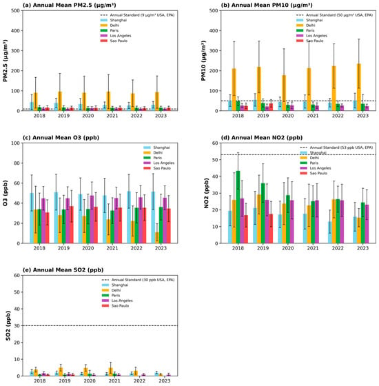
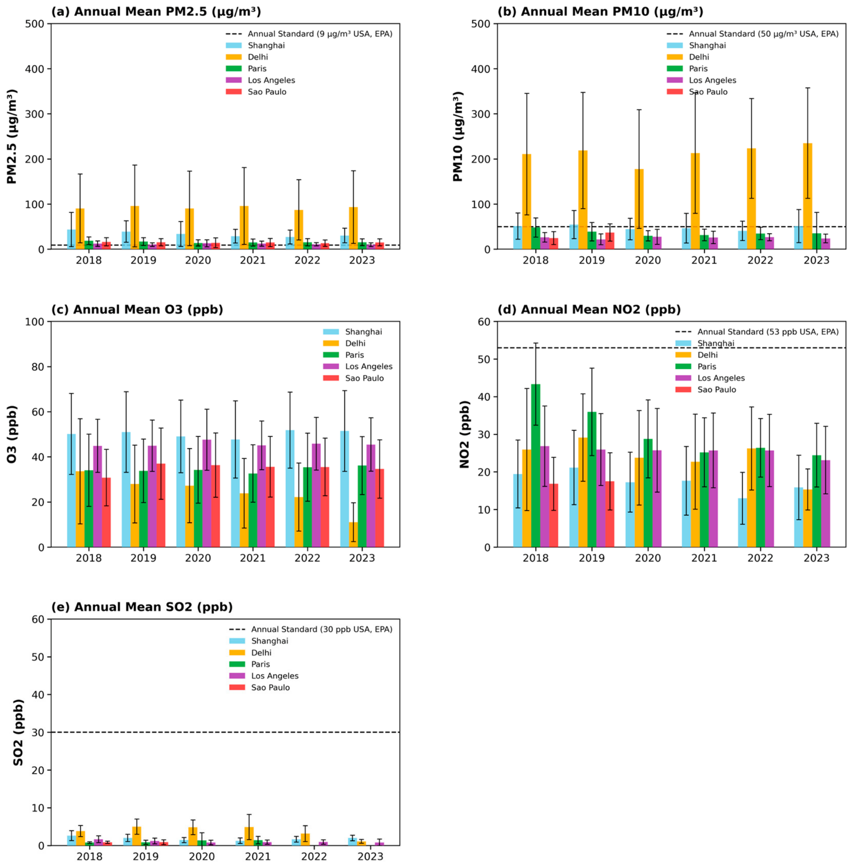
Annual mean concentrations of PM2.5, PM10, O3, NO2, and SO2 show that the five megacities followed markedly different trajectories (Figure 2). The contrast is strongest for PM2.5. Shanghai and Delhi remained substantially more polluted than Los Angeles throughout the study period, whereas Paris and São Paulo occupied an intermediate range. The multi-pollutant view also shows that reductions in primary pollutants did not necessarily coincide with comparable reductions in ozone, underscoring the different controls on directly emitted and secondary pollutants.
Figure 2.
Annual mean concentrations of (a) PM2.5, (b) PM10, (c) O3, (d) NO2, and (e) SO2 for Shanghai, Delhi, Paris, Los Angeles, and São Paulo during 2018–2023. The error bars for pollutant concentration represent one standard deviation.
Shanghai showed a clear but non-monotonic improvement in PM2.5. The annual mean decreased from 43.52 µg/m3 in 2018 to 27.02 µg/m3 in 2022, followed by a partial rebound to 30.28 µg/m3 in 2023. NO2 also declined from 19.43 in 2018 to 12.97 in 2022 before rising to 15.86 in 2023, while SO2 decreased from 2.61 in 2018 to 1.27 in 2021 and then increased to 1.98 in 2023. These simultaneous declines in PM2.5, NO2, and SO2 are consistent with broad reductions in combustion-related pollution; however, the 2023 increases indicate that the improvements were not uniformly sustained. O3 changed much less than the primary pollutants, suggesting that ozone responded to a different combination of precursor emissions, atmospheric chemistry, and meteorology.
Delhi was the most consistently polluted city in terms of annual PM2.5 levels. PM2.5 showed no steady trend, staying between 87.06 and 95.96 µg/m3 throughout the period, with no clear drop in 2020. PM10 fell to 177.61 µg/m3 in 2020 before rising to 235.00 µg/m3 by 2023. The 2020 decline in PM10 coincides with pandemic-related restrictions and so cannot be seen as a purely regulatory effect. Nitrogen dioxide (NO2) fell from 25.96 to 15.32 ppb and SO2 from 3.82 to 1.09 ppb between 2018 and 2023, showing that reductions in some precursor or combustion emissions were not enough to produce a similar sustained decrease in PM2.5.
Paris showed a more coherent long-term reduction in particulate and nitrogen dioxide concentrations. PM2.5 decreased from 18.80 µg/m3 in 2018 to 15.41 µg/m3 in 2023, PM10 fell sharply through 2020 and then stabilized, and NO2 declined from 43.31 to 24.44 over the study period. O3, however, remained comparatively stable. This divergence is important: successful reduction in NO2 and particulate matter does not automatically imply proportional reductions in O3 because ozone production depends nonlinearly on NOx, volatile organic compounds, photochemistry, and meteorological conditions.
Los Angeles had by far the lowest annual PM2.5 concentrations among the five cities. PM2.5 decreased from 12.19 µg/m3 in 2018 to 10.10 µg/m3 in 2019, rose to 13.06 µg/m3 in 2020, and then declined to 9.90 µg/m3 by 2023. The 2020 increase contrasts with the pandemic-era reductions evident in several other urban pollutant records and indicates that regional episodic sources and meteorology can outweigh reductions in routine urban activity. PM10 showed a similar 2020 increase, while NO2 and SO2 declined over the six-year period.
São Paulo differed from Shanghai, Paris, and Los Angeles because PM2.5 changed little over the study period. Concentrations decreased from 16.36 µg/m3 in 2018 to 13.26 µg/m3 in 2022 before rising to 15.09 µg/m3 in 2023. NO2 was available only for 2018 and 2019 (16.81 and 17.49 ppb, respectively), while O3 increased from 30.79 ppb in 2018 to 36.95 ppb in 2019 and then declined gradually to 34.62 ppb in 2023. The São Paulo record therefore illustrates that urban air-quality changes during 2018–2023 were not uniformly improving and that city-specific emissions and meteorological variability remain critical.
3.2. Persistence of PM2.5 and O3 Exceedances
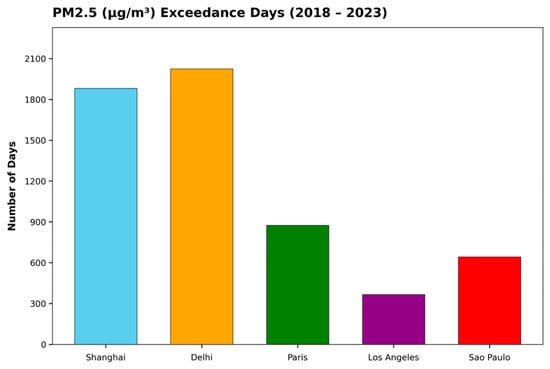
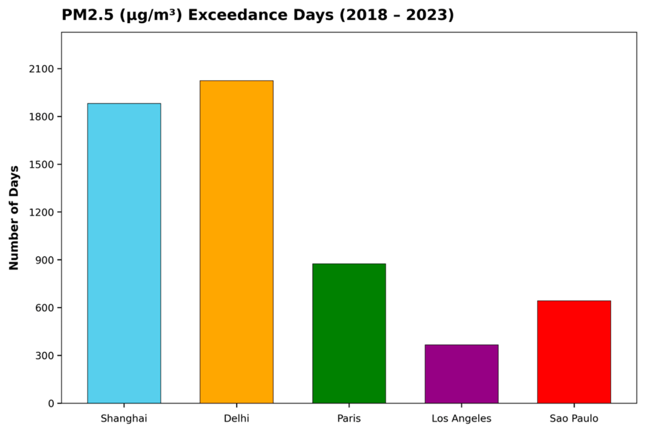
Exceedance frequency provides a complementary measure of pollution burden because a declining annual mean can coexist with many days above a health-based or regulatory threshold. Delhi recorded 2025 PM2.5 exceedance days during 2018–2023 and Shanghai recorded 1881, compared with 875 in Paris, 643 in São Paulo, and 366 in Los Angeles (Figure 3). Thus, the annual-mean improvement in Shanghai did not translate into a comparable reduction in the frequency of high-PM2.5 days. Delhi likewise remained characterized by persistent rather than episodic particulate pollution.
Figure 3.
Cumulative PM2.5 exceedance days during 2018–2023 for the five megacities.
The contrast between Los Angeles and the other cities is large. Even allowing for differences in monitoring networks and threshold definitions, the source analysis identifies a fundamentally different pollution regime. Los Angeles experiences occasional PM2.5 exceedances, whereas Shanghai and Delhi are above the selected threshold on most monitored days. Paris and São Paulo also show substantial persistence, despite lower annual PM2.5 levels than Shanghai and Delhi.
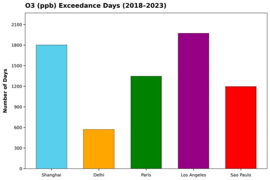
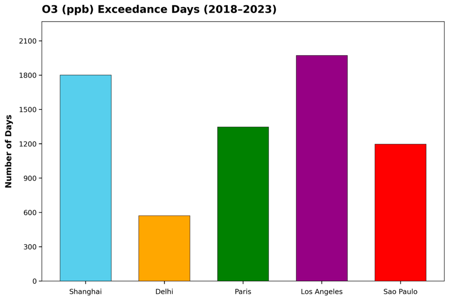
O3 exceedance frequency presents a different ranking (Figure 4). Los Angeles has the largest cumulative number of O3 exceedance days, with 1973, followed closely by Shanghai 1801, Paris 1347, and São Paulo 1196. Delhi has a smaller total of 571. The high ozone-exceedance frequency in Los Angeles despite pronounced reductions in NO2 and PM2.5 illustrates why ozone requires separate treatment from primary pollutants. O3 is produced photochemically and responds nonlinearly to changes in precursor emissions. Therefore, reductions in NO2 alone are not expected to yield a one-to-one decline in O3.
Figure 4.
Cumulative O3 exceedance days during 2018–2023 for the five megacities.
3.3. Meteorological Controls on PM2.5
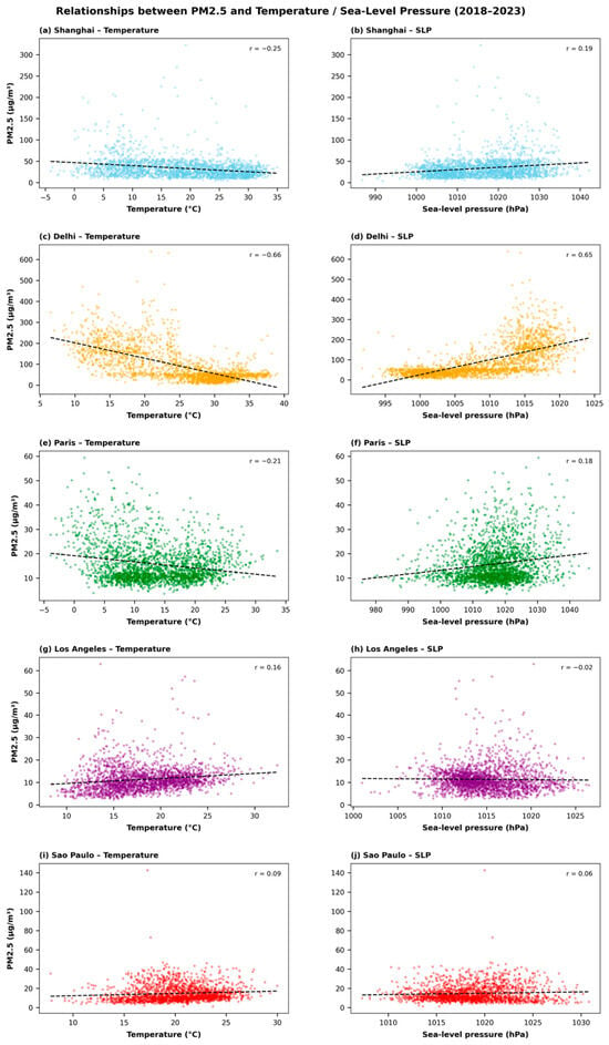
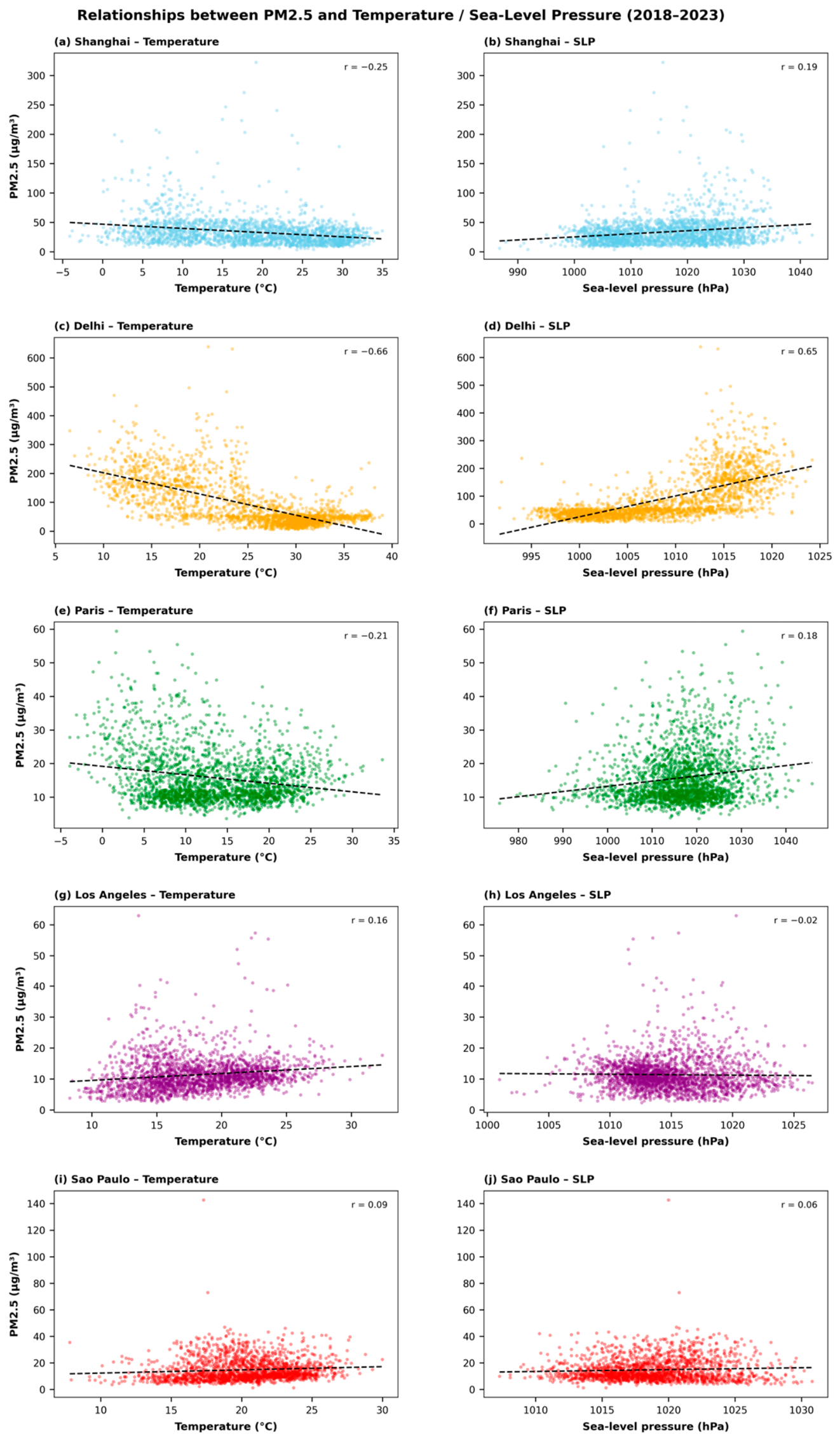
The meteorological regressions (Figure 5) show that PM2.5 does not respond uniformly to temperature, sea-level pressure (SLP), or wind speed across the five cities. The strongest relationships occur in Delhi, where temperature and SLP both indicate a pronounced seasonal/stagnation control on particulate pollution. In contrast, several relationships in Shanghai, Paris, Los Angeles, and São Paulo are weak, implying that meteorology explains only part of the observed PM2.5 variability.
Figure 5.
Relationships between temperature and Sea Level Pressure with PM2.5 for (a,b) Shanghai, (c,d) Delhi, (e,f) Paris, (g,h) Los Angeles, and (i,j) São Paulo during 2018–2023.
3.3.1. Temperature and Sea Level Pressure—PM2.5 Relationships
Temperature was negatively correlated with PM2.5 in Shanghai (r = −0.25), Delhi (r = −0.66), and Paris (r = −0.21), but weakly positively correlated in Los Angeles (r = 0.16) and São Paulo (r = 0.09). Delhi exhibits both the strongest correlation and the steepest slope, indicating that high-PM2.5 conditions are strongly associated with lower temperatures. This relationship should not be interpreted as a simple direct temperature effect. In Delhi, temperature covaries with wintertime boundary-layer depth, synoptic stagnation, humidity, seasonal emissions, and regional transport; temperature therefore acts partly as an indicator of a broader seasonal pollution regime.
Shanghai and Paris show the same sign but much weaker relationships, suggesting that temperature alone explains relatively little of the day-to-day PM2.5 variability. The weak positive relationship in Los Angeles indicates that temperature alone explains little of the PM2.5 variability, including warm-season secondary aerosol formation and episodic regional sources. São Paulo also shows only a weak positive relationship, consistent with the influence of multiple meteorological and emissions factors.
SLP provides additional evidence for the importance of stagnation in Delhi. The correlation between SLP and PM2.5 is 0.65 in Delhi, substantially stronger than in Shanghai (0.19), Paris (0.18), São Paulo (0.06), or Los Angeles (−0.02). High-pressure conditions are commonly associated with weaker synoptic ventilation and more stable lower-atmospheric conditions, so the strong positive relationship in Delhi is consistent with enhanced accumulation during stagnant episodes. When considered together with the negative temperature correlation, the results identify a coherent meteorological regime in which colder, higher-pressure conditions coincide with elevated PM2.5.
The near-zero SLP relationship in Los Angeles indicates that sea-level pressure alone is not a useful predictor of particulate concentrations there. Likewise, the weak positive correlations in Shanghai, Paris, and São Paulo suggest that SLP may modulate pollution episodes but is not the dominant control. These inter-city differences caution against transferring meteorology–pollution relationships derived for one megacity directly to another.
3.3.2. Wind Speed–PM2.5 Relationships
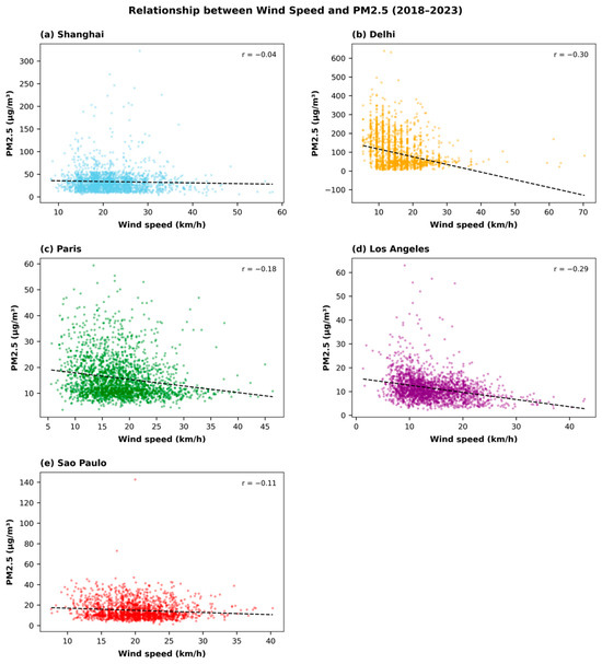
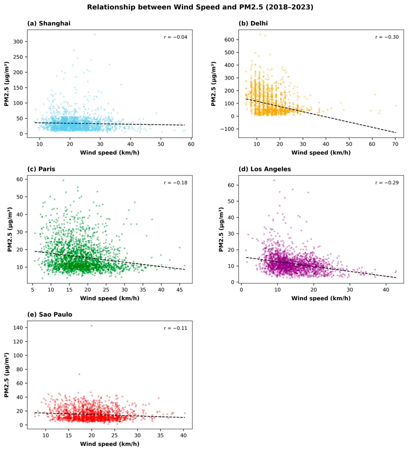
Wind speed is negatively correlated with PM2.5 in all five cities (Figure 6), consistent with enhanced dilution and ventilation at higher wind speeds. The magnitude of the relationship is largest in Delhi (r = −0.30), followed by Los Angeles (−0.29) and Paris (−0.18), and is weak in São Paulo (−0.11) and Shanghai (−0.04). The common negative sign is physically consistent with dispersion, but the relatively small correlation coefficients show that wind speed alone explains only a modest fraction of PM2.5 variability. Emission strength, atmospheric mixing depth, precipitation, humidity, chemical production, and regional transport remain important contributors.
Figure 6.
Relationships between wind speed and PM2.5 for (a) Shanghai, (b) Delhi, (c) Paris, (d) Los Angeles, and (e) São Paulo during 2018–2023.
The meteorological results therefore provide a more nuanced interpretation than a simple city ranking. Delhi is distinguished by a strong combined signature of low temperature and high pressure, whereas Los Angeles shows its clearest meteorological response to wind speed. Shanghai, Paris, and São Paulo generally show weaker one-variable relationships, indicating that their particulate variability likely emerges from interacting meteorological and emissions controls.
3.4. Temperature Dependence of Ozone
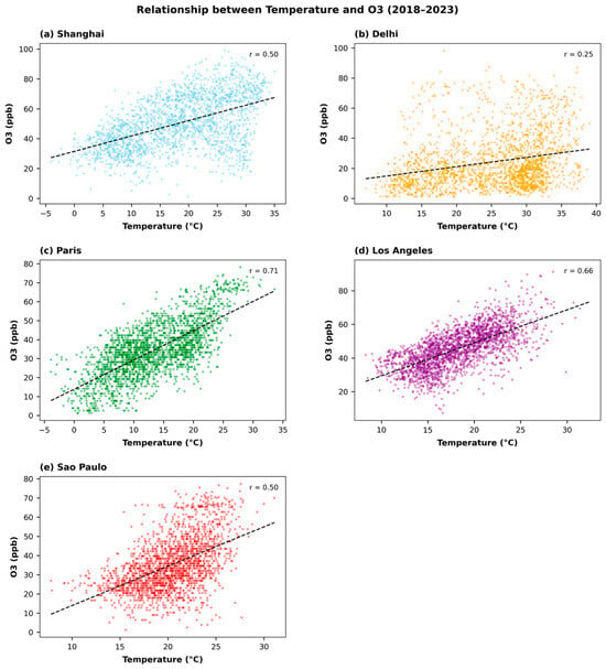
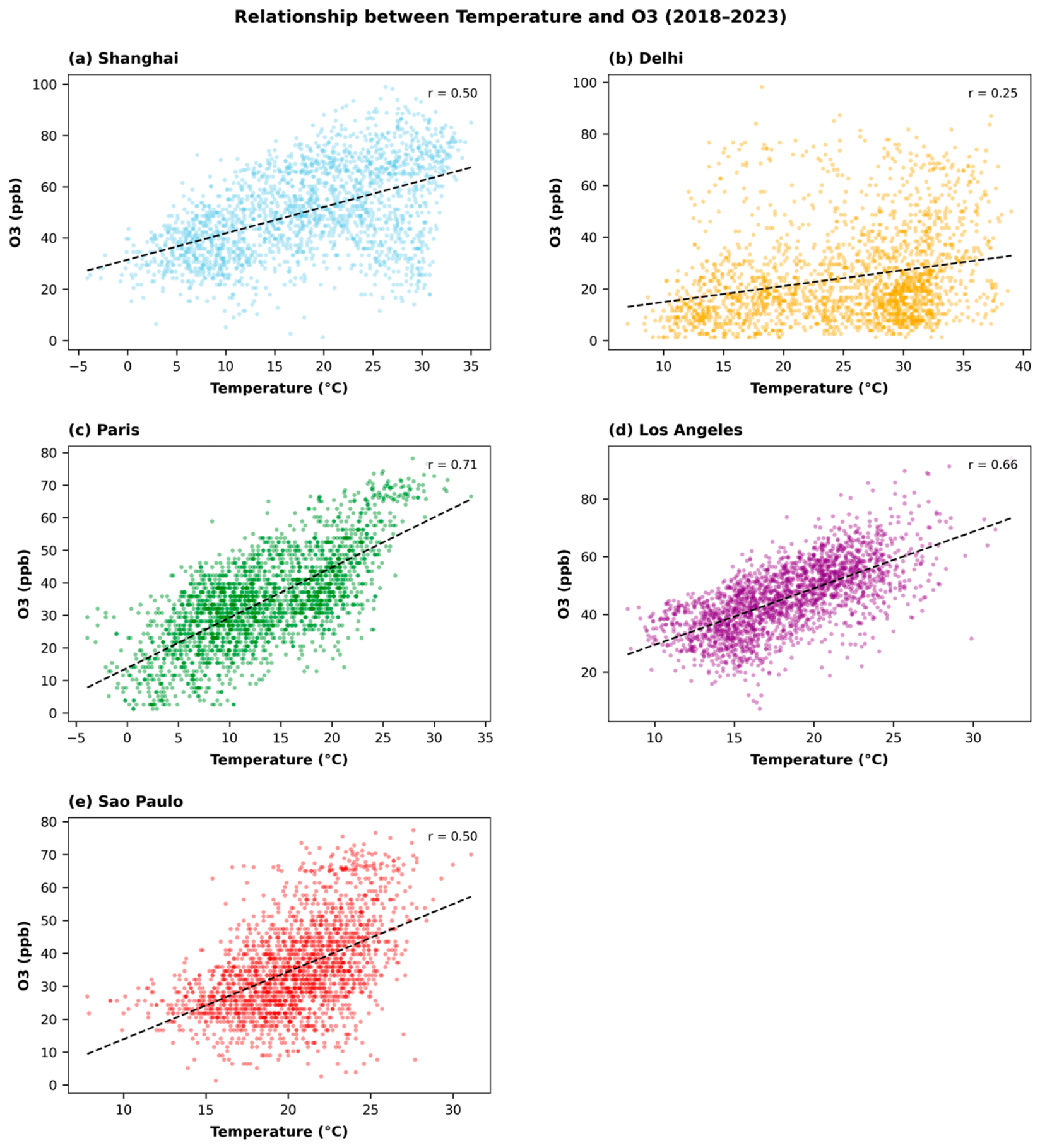
The temperature response of O3 (Figure 7) differs from that of PM2.5. Temperature is positively correlated with O3 in all five cities, with the strongest relationships in Paris (r = 0.71), Los Angeles (r = 0.66), and Shanghai and São Paulo sharing the same correlation (r = 0.50). Delhi shows a weaker positive relationship (r = 0.25). This positive response is consistent with increased photochemical ozone production under warmer, sunnier conditions, although temperature also covaries with radiation, boundary-layer dynamics, biogenic emissions, and regional transport.
Figure 7.
Relationships between temperature and O3 for (a) Shanghai, (b) Delhi, (c) Paris, (d) Los Angeles, and (e) São Paulo during 2018–2023.
Paris is particularly notable because its annual NO2 concentration declines substantially while O3 remains comparatively stable and strongly temperature sensitive. This combination suggests that changes in precursor emissions and photochemistry need to be interpreted together. Los Angeles similarly shows a strong temperature–O3 correlation despite relatively stable annual ozone concentrations, indicating that seasonal meteorology continues to organize ozone variability even where long-term mean concentrations change little.
The contrast between PM2.5 and O3 provides one of the clearest cross-pollutant results of the study. In Delhi, high PM2.5 is associated with colder, high-pressure conditions, whereas O3 tends to increase with temperature. Thus, the meteorological conditions that favor particulate accumulation are not the same as those that favor ozone formation. Effective air-quality management must therefore account for pollutant-specific chemistry and meteorology rather than relying on a single seasonal mitigation framework.
3.5. Seasonal Variability of PM2.5
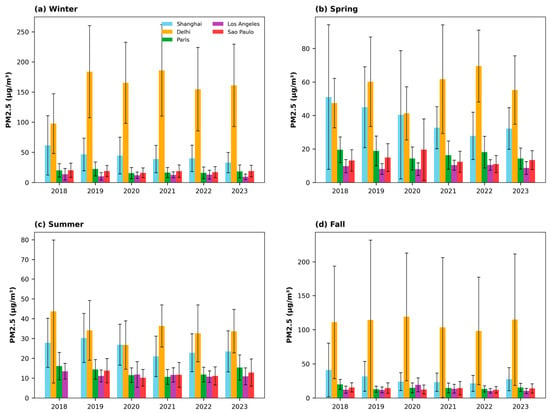
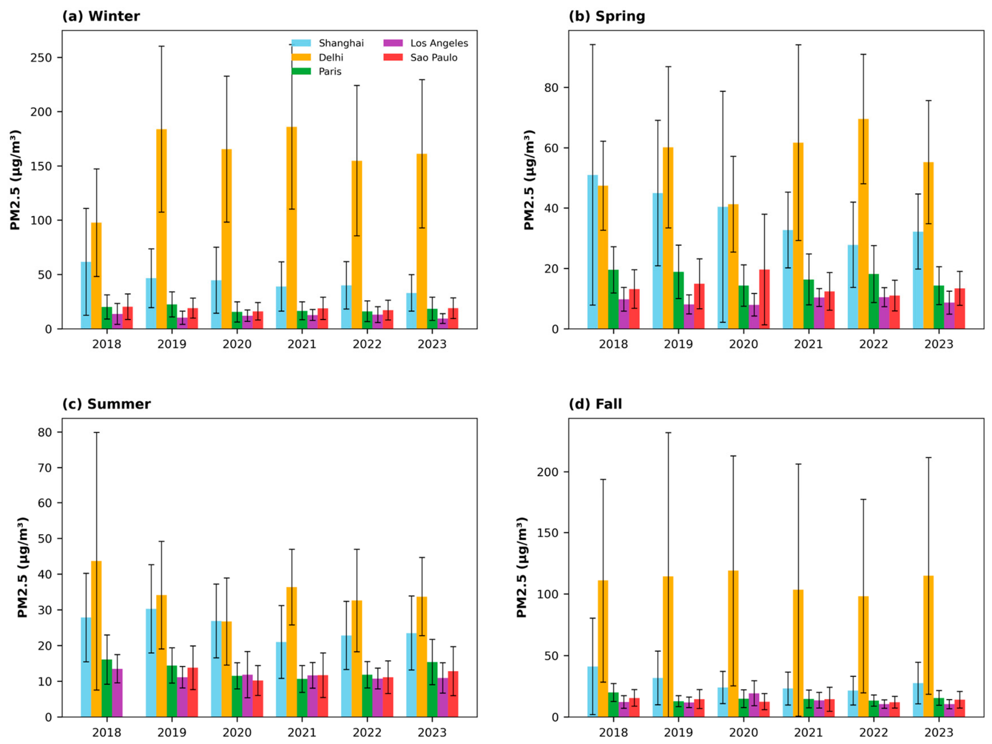
Seasonal averaging exposes patterns that are muted in annual means. Shanghai shows improvement across all seasons (Figure 8). Winter PM2.5 decreases from 61.61 µg/m3 in 2018 to 32.97 µg/m3 in 2023, spring from 51 to 32.21 µg/m3, summer from 27.84 to 23.48 µg/m3, and fall from 41.13 to 27.53 µg/m3. Despite the multi-season decline, winter and spring remain consistently more polluted than summer, indicating that seasonality persists even as the overall concentration level falls.
Figure 8.
Seasonal mean PM2.5 concentrations for the five megacities during 2018–2023. Seasons are defined as winter (December–February), spring (March–May), summer (June–August), and fall (September–November); for São Paulo, seasons are reversed to reflect the Southern Hemisphere (winter = June–August, summer = December–February). The error bars for pollutant concentration represent one standard deviation.
Delhi exhibits the strongest seasonal contrast. Winter PM2.5 is extremely high throughout the record, beginning at 97.68 µg/m3 in 2018 and reaching 161.09 µg/m3 in 2023, with a maximum of 185.95 µg/m3 in 2021. Summer concentrations are much lower, falling from 43.70 µg/m3 in 2018 to 26.72 µg/m3 in 2020 before increasing to 33.69 µg/m3 in 2023. Fall remains highly polluted, reaching 114.95 µg/m3 in 2023. The persistence of severe winter and fall pollution explains why the annual PM2.5 burden remains high despite reductions during selected seasons.
Paris shows lower seasonal PM2.5 after 2018–2019, with a particularly evident decrease during summer. Los Angeles remains much lower overall but shows an important fall anomaly in 2020, when PM2.5 reaches 19.29 µg/m3 compared with 10.46 to 13.55 µg/m3 in 2021 to 2023. This seasonal excursion is largely obscured in the annual mean and demonstrates the value of retaining seasonal diagnostics. São Paulo shows fluctuating winter and fall concentrations rather than the systematic decline seen in Shanghai; winter decreases from 20.23 µg/m3 in 2018 to 18.79 µg/m3 by 2021, while fall also remains elevated.
The cross-city comparison therefore indicates that “improvement” depends strongly on season. A city may show a favorable annual trend while retaining a recurrent high-risk season. For policy evaluation, seasonal maxima and frequency of high-concentration episodes are therefore at least as important as annual mean changes.
3.6. Seasonal Variability of Ozone
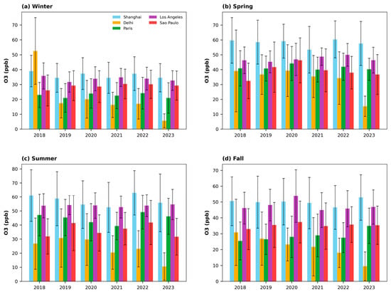
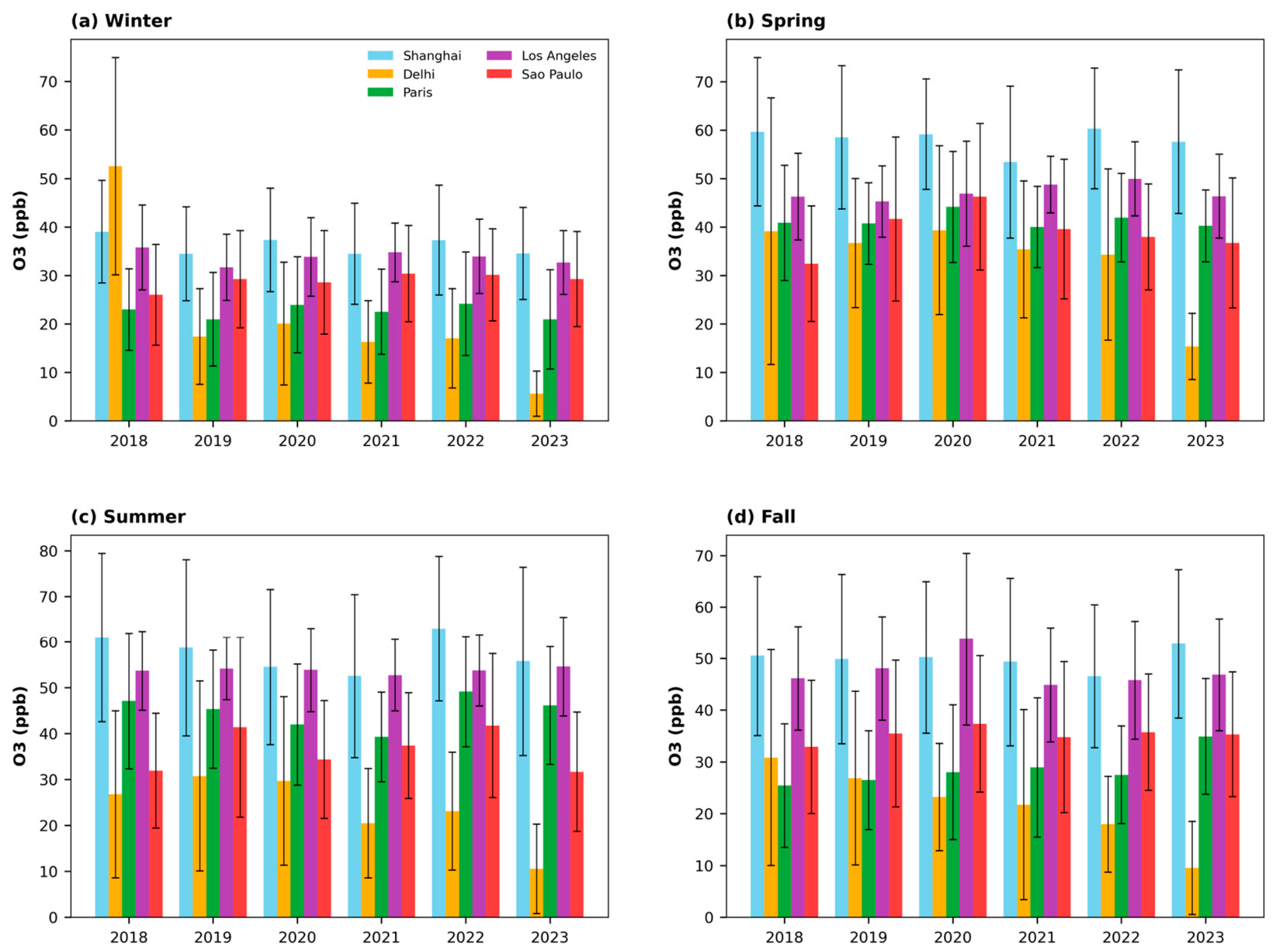
O3 exhibits a seasonal structure that is generally opposite to that of PM2.5 (Figure 9). In Shanghai, winter O3 remains near the lower end of the seasonal distribution, whereas spring and summer O3 are substantially higher. Summer concentrations begin at 60.98 in 2018, reach 62.92 in 2022, and decline to 55.78 in 2023. The warm-season maximum is consistent with stronger photochemical production under increased temperature and solar radiation.
Figure 9.
Seasonal mean O3 concentrations for the five megacities during 2018–2023. Seasons are defined as winter (December–February), spring (March–May), summer (June–August), and fall (September–November); for São Paulo, seasons are reversed to reflect the Southern Hemisphere (winter = June–August, summer = December–February). The error bars for pollutant concentration represent one standard deviation.
Delhi has more variation from year to year: in winter, the ozone level falls from 52.52 ppb in 2018 to 17.40 ppb in 2019 and stays around that figure until 2022, while in spring, it ranges between 34.32 and 39.36 ppb; in summer, the ozone level reaches a peak of 30.75 ppb in 2019 before then decreasing. In 2023, ozone drops sharply in all seasons, reaching 5.57 ppb in winter, 15.33 ppb in spring and 10.54 ppb in summer. This indicates that temperature alone is not enough to explain the ozone levels in Delhi; precursor emissions, the timing of the monsoon, cloudiness, transport, and NO titration are likely to be responsible for the observed variability.
In the warm season, Los Angeles exhibits the clearest and steadiest pattern; during winter, the O3 levels are between 31.65 and 35.77 ppb, in spring, about 45.28 to 49.97 ppb, and in summer, about 52.71 to 54.58 ppb. The consistency of this pattern lends support to the idea that photochemical seasonality remains the primary factor in determining the situation even though there is little variation in the annual average. As for São Paulo, the seasons of the Southern Hemisphere should be used, which is why its seasonal peaks occur at different times of the year than those in the cities of the Northern Hemisphere.
3.7. Integrated Interpretation of Annual, Meteorological, and Seasonal Patterns
Considered together, the annual and seasonal results show that the five megacities did not follow a single trajectory of air-quality improvement. Shanghai exhibited broad reductions in PM2.5 and several primary pollutants over much of the study period, although elevated cold-season concentrations remained evident. Delhi continued to experience the greatest particulate burden, with pronounced winter and post-monsoon enhancement. Paris showed comparatively consistent reductions in PM2.5 and NO2, whereas O3 exhibited less evidence of improvement. Los Angeles maintained substantially lower PM2.5 concentrations than the other cities but remained affected by episodic particulate enhancement and warm-season photochemical pollution. São Paulo showed a less consistent PM2.5 trajectory, distinguishing it from cities with clearer downward trends.
Seasonal analysis provided information that was not apparent from the annual means alone. Delhi and Shanghai experienced higher PM2.5 concentrations during colder periods, consistent with the combined influence of seasonal emissions and meteorological conditions unfavorable for dispersion. Paris also remained susceptible to particulate accumulation during winter stagnation, while its O3 burden was more strongly associated with warmer and sunnier conditions. Los Angeles showed a clear warm-season photochemical context together with occasional particulate episodes that may reflect wildfire smoke and other regional influences. In São Paulo, seasonal interpretation followed the Southern Hemisphere cycle, with particulate accumulation occurring more prominently during cooler and drier conditions.
The pollutant–meteorology relationships also differed among the five cities. In Delhi, the combination of a negative temperature–PM2.5 relationship and a positive sea-level-pressure–PM2.5 relationship was consistent with enhanced particulate accumulation during colder, more stagnant conditions. In Los Angeles, the wind-speed relationship suggested a comparatively stronger role for atmospheric ventilation. The weaker one-variable relationships in Shanghai, Paris, and São Paulo indicated that temperature, pressure, or wind speed alone explained only part of the observed PM2.5 variability. O3 was positively associated with temperature, although the strength of this relationship differed among the cities.
Annual means alone did not capture the seasonal and meteorological differences among the cities. Improvement in annual mean PM2.5 does not necessarily eliminate recurrent high-pollution seasons, and reductions in primary pollutants do not guarantee corresponding reductions in O3.
4. Discussion
The comparison demonstrates that urban air-quality trajectories cannot be described by a single global pattern. Differences between the five megacities reflect interactions among emissions, atmospheric chemistry, meteorology, seasonality, topography, regional transport, and regulatory history. Shanghai improved substantially in PM2.5 over 2018–2022 but experienced a 2023 rebound, indicating that long-term reductions can coexist with interannual variability. Delhi remained an extreme particulate-pollution environment despite declines in NO2 and SO2, emphasizing that reductions in selected primary pollutants do not necessarily translate into rapid PM2.5 improvement when regional burning, dust, secondary aerosol formation, and adverse winter meteorology remain important. These results are consistent with the literature identifying Delhi’s wintertime meteorology and regional emissions as major contributors to severe particulate episodes [19,20,30].
Paris and Los Angeles illustrate different stages of long-term pollution control, but different meteorological and chemical environments. Paris showed clear declines in PM2.5 and NO2 but persistent ozone behavior, underscoring the difficulty of controlling a secondary pollutant governed by nonlinear chemistry. Los Angeles maintained the lowest PM2.5 levels and fewest exceedance days, consistent with decades of vehicle and industrial emission controls, yet its relatively strong temperature–ozone correlation indicates continuing photochemical sensitivity. Basin topography, coastal circulation, high temperatures, stagnation, and wildfire smoke can all influence pollution episodes in Southern California. These patterns agree with studies highlighting air-quality benefits from emission regulation and vehicle electrification in California [26,31]. In both cities, the persistence of O3 despite reductions in some primary pollutants illustrates the nonlinear response of secondary pollution to precursor emissions and meteorological conditions.
São Paulo’s increase in PM2.5 by 2023 contrasts with the improvement in several other cities and reflects changes in emissions, meteorology, transported smoke, or secondary aerosol formation, but their individual contributions were not quantified. Prior work on São Paulo similarly emphasizes the continuing importance of secondary pollutants even after substantial reductions in primary emissions [28,29]. However, the present analysis cannot quantify the contribution of these individual factors. São Paulo consequently provides an important contrast to the assumption that particulate concentrations decline uniformly as urban emissions controls mature.
The meteorological analysis reinforces the importance of local atmospheric context. Delhi’s strong positive SLP–PM2.5 relationship and negative temperature–PM2.5 relationship are consistent with winter stagnation, shallow mixing, and pollutant accumulation. Negative wind–PM2.5 relationships across all cities reflect the expected role of ventilation and dispersion. In contrast, positive temperature–O3 relationships—especially in Paris and Los Angeles—are consistent with enhanced photochemical production under warmer conditions. Because correlations do not isolate causal mechanisms, these relationships should be interpreted as indicators of meteorological sensitivity rather than direct source attribution.
The 2018–2023 period also spans COVID-19 restrictions and subsequent recovery. The temporary perturbation in activity levels likely contributed to some 2020 anomalies, but the magnitude and direction of changes differed by pollutant and city. This is consistent with global COVID-19 studies showing widespread reductions in NO2 and particulate pollution but more heterogeneous ozone responses because of changes in precursor chemistry [11,12].
The cross-city comparison also indicates that air-quality priorities must reflect local pollutant mixtures and seasonal behavior. For Shanghai, continued reductions in combustion-related emissions should be accompanied by attention to cold-season particulate episodes and regional transport. Delhi requires coordinated year-round action on transportation, combustion, industry, dust, and waste burning, together with regional measures addressing agricultural burning and severe winter episodes. Paris must continue reducing traffic- and heating-related emissions while also considering the regional and nonlinear chemistry of warm-season O3. Los Angeles requires continued control of O3 precursors together with planning for heat, stagnation, and wildfire-smoke episodes. In São Paulo, vehicle-emission controls should be considered alongside secondary aerosol formation and regionally transported biomass-burning smoke. These implications are based on the observed patterns and supporting literature; the present study does not directly quantify the effectiveness of individual policies.
5. Strengths, Limitations, and Future Research Needs
This study applies a common analytical framework to multiple pollutants across five global megacities representing different climatic regions, emissions environments, seasonal cycles, and air-quality management histories. Rather than relying exclusively on annual mean concentrations, the analysis considers annual trends, seasonal variability, exceedance frequency, and pollutant–meteorology relationships. The inclusion of cities from Asia, Europe, North America, and South America also allows comparison across Northern and Southern Hemisphere settings. In addition, the 2018–2023 period captures conditions before, during, and after the COVID-19 disruption, providing a useful record of substantial interannual variability, although the study was not designed to isolate the effect of the pandemic.
These strengths should be considered together with several limitations that affect the interpretation and direct comparability of the results.
First, the analysis combines air-quality observations obtained from different monitoring systems. Data for Shanghai, Delhi, Paris, and São Paulo were obtained from the World Air Quality Index Project, whereas the Los Angeles data were obtained from the U.S. Environmental Protection Agency. Differences among these systems in station siting, instrument type, quality-control procedures, spatial coverage, data completeness, and reporting conventions may affect direct inter-city comparability. The observed differences should therefore be interpreted as contrasts among the datasets and urban monitoring environments represented here rather than as definitive rankings of population-wide exposure.
Second, city-level air quality is spatially heterogeneous. Concentrations measured at an individual station or a limited group of stations may not represent conditions across an entire metropolitan region. Traffic-oriented, industrial, urban-background, suburban, and regional-background stations can produce substantially different pollutant records. The geographical definitions used for the five cities also differ, ranging from central municipalities to larger metropolitan or monitoring regions. Consequently, differences among cities may partly reflect the spatial domain and monitoring locations represented in each dataset.
Third, temporal aggregation may obscure shorter pollution episodes and spatially localized events. Annual means provide a useful measure of long-term behavior but can conceal seasonal extremes, short-duration episodes, and differences in the number of valid observations. Seasonal averages and exceedance frequencies provide complementary information, but they remain sensitive to missing data, valid-day requirements, and the selected averaging periods. The use of a common health-based threshold facilitates comparison among cities but should not be interpreted as an assessment of compliance with the legally applicable air-quality standards in each country.
Fourth, the statistical analyses identify associations rather than causal relationships. Temperature, sea-level pressure, and wind speed covary with season, boundary-layer structure, humidity, precipitation, emissions, atmospheric chemistry, and regional transport. Bivariate correlations cannot isolate the independent effect of an individual meteorological variable or determine whether an observed pollutant change resulted from meteorology, emissions, policy interventions, or their combined influence. The relationships reported here should therefore be interpreted as indicators of meteorological sensitivity rather than direct measures of causation.
Fifth, several potentially important explanatory variables were not included in the statistical analysis. These include relative humidity, precipitation, solar radiation, planetary boundary-layer height, atmospheric stability, wildfire and agricultural-burning activity, emissions inventories, and regional air-mass transport. Their omission limits the ability to explain individual pollution episodes and to distinguish locally emitted pollution from secondary formation and transported contributions.
Future research should build on this comparative framework by using longer observational records, consistent station classifications, explicit data-completeness criteria, and spatially resolved monitoring information. Multivariable statistical or process-based modeling could help separate the effects of meteorology, emissions, atmospheric chemistry, and regional transport. Incorporating emissions inventories, boundary-layer characteristics, air-mass trajectories, satellite observations, and source-apportionment information would support a more mechanistic comparison among megacities. Despite its limitations, the present study analyzes cross-city contrasts and provides a basis for developing more detailed investigations of the processes governing particulate matter and ozone in different urban environments. Future studies can test these cross-city differences using consistent station classifications, longer records, emissions inventories, and atmospheric-transport analyses.
6. Conclusions
This study compared annual and seasonal air-quality patterns and their meteorological associations across Shanghai, Delhi, Paris, Los Angeles, and São Paulo during 2018–2023. The results demonstrate that the five megacities did not follow a uniform trajectory of air-quality change. Shanghai showed an overall reduction in PM2.5 and several primary pollutants, although seasonal particulate pollution remained evident. Delhi continued to experience the most persistent particulate burden, particularly during colder and more stagnant periods. Paris showed reductions in PM2.5 and NO2 but less improvement in O3, while Los Angeles maintained comparatively low PM2.5 concentrations but remained affected by photochemical O3 and episodic particulate pollution. São Paulo exhibited a less consistent PM2.5 trend, emphasizing that improvements observed in some cities cannot be generalized across different urban environments.
The comparison further shows that annual mean concentrations alone do not fully characterize urban air quality. Seasonal variability, elevated-pollution episodes, and meteorological conditions provide important complementary information, while the differing behavior of PM2.5 and O3 demonstrates the need for pollutant-specific interpretation. Effective air-quality management must therefore account for local emissions, atmospheric chemistry, climate, seasonality, topography, and regional transport. Longer and more spatially consistent observational records, combined with emissions information and multivariable or process-based analyses, will be needed to distinguish the effects of policy, meteorology, and regional transport more clearly across megacities.
Author Contributions
V.P.A., S.S. and I.A. contributed to the study conception and design. Material preparation, data collection, and analysis were performed by I.A., V.P.A. and S.S. All authors have read and agreed to the published version of the manuscript.
Funding
This research received no external funding.
Institutional Review Board Statement
Not applicable.
Informed Consent Statement
Not applicable.
Data Availability Statement
Air-quality data sources are described in Section 2.1.
Acknowledgments
We would like to thank the Kingdom of Saudi Arabia for providing one of the co-authors (I.A.) with the Kingdom of Saudi Arabia Fellowship.
Conflicts of Interest
The authors declare no conflicts of interest.
References
- Uttamang, P.; Aneja, V.P.; Hanna, A.F. Assessment of gaseous criteria pollutants in the Bangkok Metropolitan Region, Thailand. Atmos. Chem. Phys. 2018, 18, 12581–12593. [Google Scholar] [CrossRef] [Scilit]
- Uttamang, P.; Campbell, P.C.; Aneja, V.P.; Hanna, A.F. A multi-scale model analysis of ozone formation in the Bangkok Metropolitan Region, Thailand. Atmos. Environ. 2020, 229, 117433. [Google Scholar] [CrossRef] [Scilit]
- Vilcins, D.; Christofferson, R.C.; Yoon, J.-H.; Nazli, S.N.; Sly, P.D.; Cormier, S.A.; Shen, G. Updates in air pollution: Current research and future challenges. Ann. Glob. Health 2024, 90, 9. [Google Scholar] [CrossRef] [Scilit] [PubMed]
- Landrigan, P.J.; Fuller, R.; Acosta, N.J.R.; Adeyi, O.; Arnold, R.; Basu, N.; Baldé, A.B.; Bertollini, R.; Bose-O’Reilly, S.; Boufford, J.I.; et al. The Lancet Commission on pollution and health. Lancet 2018, 391, 462–512, Erratum in Lancet 2018, 391, 430. [Google Scholar] [CrossRef] [Scilit] [PubMed]
- Molina, M.J.; Molina, L.T. Megacities and atmospheric pollution. J. Air Waste Manag. Assoc. 2004, 54, 644–680. [Google Scholar] [CrossRef] [Scilit] [PubMed]
- Baklanov, A.; Molina, L.T.; Gauss, M. Megacities, air quality and climate. Atmos. Environ. 2016, 126, 235–249. [Google Scholar] [CrossRef] [Scilit]
- Sicard, P.; Agathokleous, E.; Anenberg, S.C.; De Marco, A.; Paoletti, E.; Calatayud, V. Trends in urban air pollution over the last two decades: A global perspective. Sci. Total Environ. 2023, 858, 160064. [Google Scholar] [CrossRef] [Scilit] [PubMed]
- Aneja, V.P.; Yoder, G.T.; Arya, S.P. Ozone in the urban southeastern United States. Environ. Pollut. 1992, 75, 39–44. [Google Scholar] [CrossRef] [Scilit] [PubMed]
- Kumar, P.; Khare, M.; Harrison, R.M.; Bloss, W.J.; Lewis, A.; Coe, H.; Morawska, L. New directions: Air pollution challenges for developing megacities like Delhi. Atmos. Environ. 2015, 122, 657–661. [Google Scholar] [CrossRef] [Scilit]
- Bray, C.D.; Nahas, A.; Battye, W.H.; Aneja, V.P. Impact of lockdown during the COVID-19 outbreak on multi-scale air quality. Atmos. Environ. 2021, 254, 118386. [Google Scholar] [CrossRef] [Scilit] [PubMed]
- Gkatzelis, G.I.; Gilman, J.B.; Brown, S.S.; Eskes, H.; Gomes, A.R.; Lange, A.C.; McDonald, B.C.; Peischl, J.; Petzold, A.; Thompson, C.R.; et al. The global impacts of COVID-19 lockdowns on urban air pollution: A critical review and recommendations. Elem. Sci. Anthr. 2021, 9, 00176. [Google Scholar]
- Liu, F.; Wang, M.; Zheng, M. Effects of COVID-19 lockdown on global air quality and health. Sci. Total Environ. 2021, 755, 142533. [Google Scholar] [CrossRef] [Scilit] [PubMed]
- He, J.; Gong, S.; Yu, Y.; Yu, L.; Wu, L.; Mao, H.; Song, C.; Zhao, S.; Liu, H.; Li, X.; et al. Air pollution characteristics and their relation to meteorological conditions during 2014–2015 in major Chinese cities. Environ. Pollut. 2017, 223, 484–496. [Google Scholar] [CrossRef] [Scilit] [PubMed]
- Zhao, D.; Chen, H.; Sun, X.; Shi, Z. Spatio-temporal Variation of PM2.5 Pollution and its Relationship with Meteorology among Five Megacities in China. Aerosol Air Qual. Res. 2018, 18, 2318–2331. [Google Scholar] [CrossRef] [Scilit]
- Zhang, H.; Wang, Y.; Hu, J.; Ying, Q.; Hu, X. Relationships between meteorological parameters and criteria air pollutants in three megacities in China. Environ. Res. 2015, 140, 242–254. [Google Scholar] [CrossRef] [Scilit] [PubMed]
- Alvim, D.S.; Herdies, D.L.; Corrêa, S.M.; Basso, L.S.; Khalid, B.; Silva, G.F.; Oyerinde, G.; de Carvalho, N.A.; Coelho, S.M.; Figueroa, S.N. COVID-19 Pandemic: Impacts on Air Quality during Partial Lockdown in the Metropolitan Area of São Paulo. Remote Sens. 2023, 15, 1262. [Google Scholar] [CrossRef] [Scilit]
- Chen, Z.; Chen, D.; Zhao, C.; Kwan, M.; Cai, J.; Zhuang, Y.; Zhao, B.; Wang, X.; Chen, B.; Yang, J.; et al. Influence of meteorological conditions on PM2.5 concentrations across China: A review of methodology and mechanism. Environ. Int. 2020, 139, 105558. [Google Scholar] [CrossRef] [Scilit] [PubMed]
- Liu, N.; Zhou, S.; Liu, C.; Guo, J. Synoptic circulation pattern and boundary layer structure associated with PM2.5 during wintertime haze pollution episodes in Shanghai. Atmos. Res. 2019, 228, 186–195. [Google Scholar] [CrossRef] [Scilit]
- Singh, B.P.; Singh, D.; Kumar, K.; Jain, V.K. Study of seasonal variation of PM2.5 concentration associated with meteorological parameters at residential sites in Delhi, India. J. Atmos. Chem. 2021, 78, 161–176. [Google Scholar] [CrossRef] [Scilit]
- Guttikunda, S.K.; Dammalapati, S.K.; Pradhan, G.; Krishna, B.; Jethva, H.T.; Jawahar, P. What Is Polluting Delhi’s Air? A Review from 1990 to 2022. Sustainability 2023, 15, 4209. [Google Scholar] [CrossRef] [Scilit]
- Kajino, M.; Ishijima, K.; Ching, J.; Yamaji, K.; Ishikawa, R.; Kajikawa, T.; Singh, T.; Nakayama, T.; Matsumi, Y.; Kojima, K.; et al. Impact of post monsoon crop residue burning on PM2.5 over North India: Optimizing emissions using a high-density in situ surface observation network. EGUsphere 2024, 2024, 1–40. [Google Scholar] [CrossRef] [Scilit]
- Gurjar, B.R. Air pollution in India: Major issues and challenges. Energy Future, 5 April 2021.
- Salama, A.M.; Patil, M.P.; MacLean, L. Urban resilience and sustainability through and beyond crisis – evidence-based analysis and lessons learned from selected European cities. Smart Sustain. Built Environ. 2023, 13, 444–470. [Google Scholar] [CrossRef] [Scilit]
- Jury, M.R. Meteorology of air pollution in Los Angeles. Atmos. Pollut. Res. 2020, 11, 1226–1237. [Google Scholar] [CrossRef] [Scilit]
- Li, Y.; Ravi, V.; Heath, G.; Zhang, J.; Vahmani, P.; Lee, S.-M.; Zhang, X.; Sanders, K.T.; Ban-Weiss, G.A. Air quality and public health co-benefits of 100% renewable electricity adoption and electrification pathways in Los Angeles. Environ. Res. Lett. 2024, 19, 34015. [Google Scholar] [CrossRef] [Scilit]
- Mousavinezhad, S.; Choi, Y.; Khorshidian, N.; Ghahremanloo, M.; Momeni, M. Air quality and health co-benefits of vehicle electrification and emission controls in the most populated United States urban hubs: Insights from New York, Los Angeles, Chicago, and Houston. Sci. Total Environ. 2024, 912, 169577. [Google Scholar] [CrossRef] [Scilit] [PubMed]
- Chiquetto, J.B.; Ynoue, R.Y.; Ibarra-Espinosa, S.A.; Ribeiro, F.N.D.; Cabral-Miranda, W.; Silva, M.E.S. Ozone Pollution and Urban Mobility Scenarios in the São Paulo Megacity. Ambiente Soc. 2020, 23, e00082. [Google Scholar] [CrossRef] [Scilit]
- Chiquetto, J.B.; Silva, M.E.S.; Cabral-Miranda, W.; Ribeiro, F.N.D.; Ibarra-Espinosa, S.A.; Ynoue, R.Y. Air Quality Standards and Extreme Ozone Events in the São Paulo Megacity. Sustainability 2019, 11, 3725. [Google Scholar] [CrossRef] [Scilit]
- Andrade, M.d.F.; Kumar, P.; de Freitas, E.D.; Ynoue, R.Y.; Martins, J.; Martins, L.D.; Nogueira, T.; Perez-Martinez, P.; de Miranda, R.M.; Albuquerque, T.; et al. Air quality in the megacity of São Paulo: Evolution over the last 30 years and future perspectives. Atmos. Environ. 2017, 159, 66–82. [Google Scholar] [CrossRef] [Scilit]
- Sanyal, S.; Wuebbles, D.J. The potential impact of a clean energy society on air quality. Earth’s Future 2022, 10, e2021EF002558. [Google Scholar] [CrossRef] [Scilit]
- Skipper, T.N.; Lawal, A.S.; Hu, Y.; Russell, A.G. Air quality impacts of electric vehicle adoption in California. Atmos. Environ. 2023, 294, 119492. [Google Scholar] [CrossRef] [Scilit]
Disclaimer/Publisher’s Note: The statements, opinions and data contained in all publications are solely those of the individual author(s) and contributor(s) and not of MDPI and/or the editor(s). MDPI and/or the editor(s) disclaim responsibility for any injury to people or property resulting from any ideas, methods, instructions or products referred to in the content. |
© 2026 by the authors. Licensee MDPI, Basel, Switzerland. This article is an open access article distributed under the terms and conditions of the Creative Commons Attribution (CC BY) license.