Abstract
The 27-day oscillation in total electron content (TEC) is analysed by means of world maps of TEC. The TEC maps are derived from measurements of the ground receiver network of the Global Navigation Satellite System (GNSS) and are provided by the International GNSS Service (IGS). The observed 27-day oscillation in TEC is mainly due to the 27-day solar rotation period, which induces a 27-day oscillation in extreme ultraviolet radiation (EUV) of the Sun. Analysing the time interval from 2003 to 2020, cross-correlation of the 27-day oscillation of the solar MgII-index of the Solar Radiation and Climate Experiment (SORCE) and the 27-day oscillation in TEC shows an average time delay of about 1.1 days for the ionospheric response with respect to the solar EUV variation. The average correlation coefficient of the solar and the ionospheric variation is 0.85. The cross-correlation of the 27-day oscillation in solar radio flux F10.7 and the 27-day oscillation in TEC gives a time lag of about 1.3 days and an average correlation coefficient of 0.78. The world maps of the amplitude of the 27-day oscillation in TEC are discussed for the TEC data from 1998 to 2024. Finally, TEC composites are derived for F10.7 enhancement events and geomagnetic storms.
1. Introduction
The ionospheric plasma of the Earth strongly depends on the ionisation of atmospheric oxygen, O2, NO, and other molecules by the extreme ultraviolet (EUV) radiation of the Sun. Temporal variations of EUV are partly mirrored in the variability of the electron density of the ionosphere. One of the most pronounced variations of the EUV radiation is the 27-day oscillation, which is related to the mean solar rotation period of about 27.3 days. Active regions of the Sun are associated with the occurrence of faculae and limb brightening. The active regions rotate within a period of about 27 days and induce a periodic increase and decrease of EUV. Over the past few decades, the total electron content (TEC) of the Earth’s ionosphere has been monitored by the worldwide network of ground-based receivers for radio signals of the Global Navigation Satellite System (GNSS). Afraimovich et al. [1] introduced the parameter global electron content (GEC) in order to track the solar activity in EUV. They found that the 11-year and 27-day oscillations of GEC are closely related to those of EUV. The variations of GEC usually lag 2 days after those of solar radio flux F10.7 cm or EUV (e.g., estimated by the solar activity proxy MgII index). Other studies indicated that the electron content of the ionosphere not only depends on the Sun but also on transport processes, dynamic and electrodynamic processes, atmospheric composition changes, and geomagnetic activity of the Earth’s system [2,3].
Simulations of Ren et al. [3] show that the time delay between the EUV variation and the associated TEC variation is between 0.5 and 0.8 days. The time delay of the TEC response to solar EUV variation is mainly due to the time delays of the thermospheric temperature and the composition ratio of O to N2, which influence the loss of ions by recombination. There is a tendency for the time delay to be a bit larger at higher geographic latitudes. The authors also obtained a good agreement with observations from the CHAMP satellite with time delays between 0.8 and 1.0 days. Observational time delays in the past literature are from 0.15 days to 4 days [3]. A new observational study [4] reported a time delay of 1 day for the 27-day oscillation of TEC with respect to the EUV variation. Another observational study by [5] mostly show time delays between 1 and 2 days. However, the time delays observed for the electron density variation in the Southern Hemisphere is 1 day larger compared to those of the Northern Hemisphere. Such a large asymmetry between the time lag of the hemispheres was not simulated by [3]. A new study of [6] emphasised that the time delays of the thermospheric parameter temperature and N2 is larger by half a day and longer compared to the response of O. Since the ionospheric electron density also depends on the ratio between O and N2, the response of the ionosphere–thermosphere system to EUV variations requires a detailed study, as conducted by [6].
The past observational studies of the time delay of TEC gave different results and some of the results such as the asymmetric response of the ionosphere in the Northern and Southern Hemispheres have not been understood yet. Thus, it is important to conduct more data analyses of the observations in order to be sure which effects are real and which effects might be due to limited accuracies of observation or data analysis. In the present study, the worldwide TEC observations from 1998 to 2024 are evaluated. The correlations and time delays are derived with respect to F10.7 and the MgII index. The characteristics of the 27-day oscillation in TEC are derived for the time interval from 1998 to 2024. Besides the cross-correlation technique, we also apply the composite analysis in order to find the peak response of TEC with respect to EUV enhancements. For comparison, the peak response of TEC to geomagnetic storms is derived.
Section 2 describes the datasets and data analysis methods which are used in the present study. Section 3 presents the results about correlation, time delay, and characteristics of the 27-day oscillations in TEC and EUV as well as the results of the composite analysis. Section 4 contains the discussion of the results. Conclusions are given in Section 5.
2. Datasets and Data Analysis
2.1. GNSS TEC Maps
The ground stations of the Global Navigation Satellite System (GNSS) receive the GNSS satellite radio signals. The ionospheric dispersion of the radio signals with different frequencies allow the derivation of TEC along the radio path. The International GNSS Service (IGS) processes world maps of TEC since June 1998. The spatial resolution of the TEC maps is 5 degrees in longitude and 2.5 degrees in latitude, while the time resolution is 2 h. The final TEC maps of IGS are based on TEC estimations from different independent analytical centres worldwide, which have slightly different retrieval software [7]. The present study utilises TEC data from the time between June 1998 and October 2024. The calculation and the error estimation of the TEC maps are described in [7]. Cross-validation with coincident satellite altimeter observations showed that the relative error of of the TEC maps of IGS is less than 20% [7].
The long-term time series of the TEC maps of IGS is approriate for studies of the solar cycle effect on TEC [2]. Lean et al. [2] emphasised that the the quality of the regular IGS TEC maps is weekly controlled by comparison of the slant TEC results from the individual data centres for a subset of permanent GNSS stations. Further intercomparisons of IGS TEC with TEC from satellite altimeters ensure in addition that possible inhomogeneities in the IGS TEC series due to changing algorithms of the data processing and changes of technical instruments are revealed and minimised. Of course, it remains a question if the IGS TEC series is sufficiently homogeneous for a trend study of TEC. A recent study by [8] derived a negative TEC trend (without solar EUV effect) using the IGS TEC series from 1999 to 2023. A negative TEC trend would align with the greenhouse effect hypothesis. The present study only focuses on the average behaviour of the 27-day oscillation of TEC. We do not derive a trend of the 27-day oscillation of TEC.
2.2. Solar EUV Proxies
An accurate measurement of solar EUV with a high temporal resolution and over a long time interval is still a challenge. Here, we utilise the long-term series of 10.7 cm solar radio flux F10.7, which is a good proxy for solar activity and solar EUV [9]. F10.7 is measured about three times around noon at the Dominion Radio Astrophysical Observatory in British Columbia. Noon corresponds there to a universal time of 20:00 UTC. We take the daily values of F10.7, which are distributed by NASA’s Omniweb, and add the 20:00 UTC information about the exact measurement time, which is not provided in the Omniweb data files. Then, we bandpass-filtered the series of daily values of F10.7 and obtained the 27-day oscillation of TEC with a sampling time of 1 day. For a better determination of the time delay by cross-correlation, the 27-day oscillation of F10.7 is linearly interpolated to the time grid of the 2 hourly TEC measurements. Since the bandpass-filtered 27-day oscillation of the daily values contains no high frequency noise, we can be sure that the interpolation process does not produce artificial maxima. The interpolation process cannot avoid a timing error due to the coarse sampling of the original F10.7 data. However, since the phase of the 27-day oscillation in F10.7 is variable from one solar activity event to the next, we assume that the undesired effect of the timing error (imperfect determination of the exact position of the maximum of 27-day oscillation in F10.7) is smoothed out in the long-term average of the time delay between the 27-day oscillation in F10.7 and TEC. The derived average value of the time delay should be accurate since the cross-correlation is computed over a long time interval (e.g., 2003–2020) with many different solar activity events.
A higher time resolution of a solar EUV proxy is provided by about 1.3 hourly data of the solar MgII index estimated from observations of the SOlar Radiation and Climate Experiment (SORCE) [10]. This data series is limited to the time interval from 5 March 2003 to 24 February 2020. We took this time interval for the correlation analyses of TEC with respect to both F10.7 and the MgII index of SORCE.
2.3. Data Analysis
The correlation coefficients and the time delays are determined by means of cross-correlation analysis between the bandpass-filtered 27-day variations of solar EUV and TEC. The digital non-recursive, finite impulse response bandpass filter is run in forward and reverse directions, so that zero-phase filtering is ensured. The filter uses a Hamming window. The number of filter coefficients is equal to a time window of three times of the central period. Thus, the bandpass filter has a fast response time to temporal changes in the data series. The bandpass cut-off frequencies are at the frequency of 1/27.3 days ± 20% (27.3 days is the Carrington solar rotation period). The calculation of the envelope of the 27.3-day oscillation amplitude of the filtered ΔTEC series and details of the bandpass filtering technique were described by Studer et al. [11].
The composite analysis is performed by the selection of local maxima or local minima in the time series of F10.7 and in the time series of the geomagnetic storm time index Dst, respectively. Dst is obtained from NASA’s Omniweb with a time resolution of 1 h. The time positions of the local maxima are utilised as timing marks for the superposed epoch analysis. The composites are restricted to moderate and strong events (Dst < −60 nT, F10.7 > 100 sfu).
3. Results
3.1. Results of the FFT and Cross-Correlation Analysis
The 27-day oscillation is visible as a broad peak in the FFT amplitude spectrum of F10.7 in Figure 1a. The broad peak is due to the differential rotation of the Sun with short rotation periods at the equator and long rotation periods at high latitudes. Further, the episodic occurrence of active regions on the Sun over short intervals (about 30 to 60 days) contributes to the broadening of the 27.3-day spectral line. Figure 1b shows the 27.3 day spectral peak of TEC observed over Ecuador (0° N, 80° W). Both FFT spectra are taken for the time interval from July 1998 to October 2024. The grey shaded area shows the range of the bandpass filter and the central period of the bandpass is indicated by the dashed vertical red line at 1/(27.3 days).
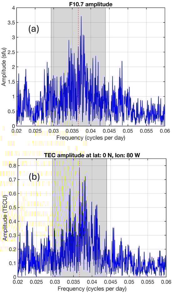
Figure 1.
FFT amplitude spectra: broad spectral peaks of the 27-day oscillation in (a) solar radio flux at 10.7 cm (F10.7) and (b) TEC above Ecuador (0° N, 80° W) for the time interval July 1998 to October 2024. The shaded region shows the selected band pass width with a central period of 27.3 days (vertical red dashed line).
The cross-correlation is calculated between the bandpass-filtered TEC series and those of F10.7 and the MgII index. Maximal correlation occurs at a certain time lag where the correlation coefficient has the maximum. The time lag for the maximal correlation corresponds to the time delay of the TEC response with respect to the 27-day variation of F10.7 or the MgII index. Figure 2 shows the world maps of maximal correlation. The correlation of TEC with respect to F10.7 in Figure 2a is smaller than those of TEC with respect to the MgII index in Figure 2b. The global average of the correlation coefficient is 0.78 for TEC and F10.7 and 0.85 for TEC and the MgII index. Generally, the correlation is higher at low latitudes than at high latitudes.
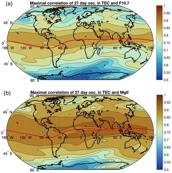
Figure 2.
Maximal correlation of the 27-day oscillations in TEC and F10.7 (a) and in TEC and the MgII index (b) for the time interval from March 2003 to February 2020. The red line indicates the geomagnetic equator.
The time delay of TEC with respect to F10.7 is 1.3 days for the global average in Figure 3a. The minimal lag is 0.75 days while the average at low latitudes (10 S to 10 N) is 1.0 days. The maximal time delay is 2.5 days. The time delay of TEC with respect to the MgII index is 1.1 days for the global average in Figure 3b. The minimal lag is 0.7 days while the average at low latitudes is 0.9 days. The maximal lag is 2.1 days. It is obvious that for both, F10.7 and the MgII index, the time delay in the Southern Hemisphere is greater than in the Northern Hemisphere. In the case of TEC and the MgII index, the time lag is 1.3 days in the Southern Hemisphere and 1.0 days in the Northern Hemisphere. In the case of TEC and F10.7, the time lag is 1.5 days in the Southern Hemisphere and 1.1 days in the Northern Hemisphere.
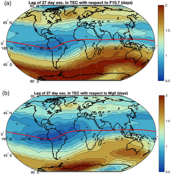
Figure 3.
Lag of the 27-day oscillations in TEC with respect to those of F10.7 (a) or the MgII index (b) for the time interval from March 2003 to February 2020. The red line indicates the geomagnetic equator.
The amplitude series of the 27-day oscillation in F10.7 and TEC (over Kenya) are shown in Figure 4. The curves are modulated by the 11-year solar cycle. The TEC amplitude are between 1 and 7 TECU and can rapidly change on time scales of about an half year. A correlation between the amplitude series of F10.7 and TEC is present.
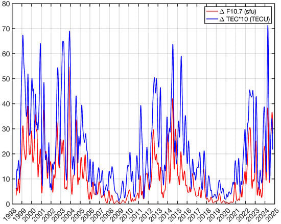
Figure 4.
Amplitude of the 27-day oscillation in F10.7 (red) and TEC (blue). The TEC amplitude series is for Kenya (0° N, 40° E). The TEC amplitude can reach 6 to 7 TECU.
As an example, we show the world map of the amplitude of the 27-day oscillation in TEC (temporal average for November and December 2003, which is centred at 1 December 2003) in Figure 5 when the 27-day oscillation reached values of about 8 TECU over the Asian and Australian longitude sector.
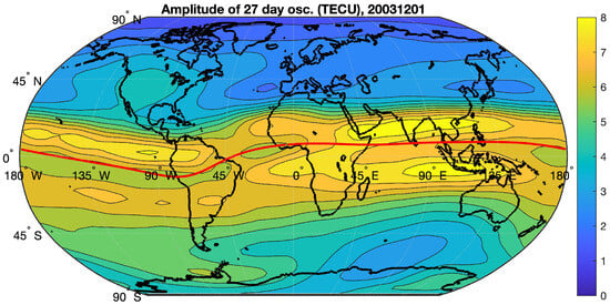
Figure 5.
World map of the amplitude of the 27-day oscillation in TEC (average for November and December 2003) when the 27-day oscillation was strong. The red line indicates the geomagnetic equator.
The mean amplitude of the 27-day oscillation in TEC in Figure 6 is less than 3 TECU averaged for the time interval from 1998 to 2024. The absolute values are strong around the equatorial ionisation anomaly (EIA).
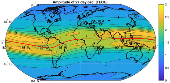
Figure 6.
World map of the mean amplitude of the 27-day oscillation in TEC averaged for the time interval from 1998 to 2024. The red line indicates the geomagnetic equator.
A different impression is obtained in Figure 7, which shows the relative amplitude of the 27-day oscillation in TEC with respect to the TEC average at each grid point (averaged for the interval from 1998 to 2024). High amplitude values of about 10% are reached in the polar zones at high geomagnetic latitudes.
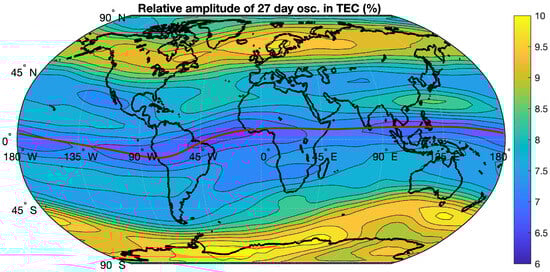
Figure 7.
World map of the mean relative amplitude of the 27-day oscillation in TEC averaged for the time interval from 1998 to 2024 (with respect to mean TEC at latitude and longitude of the grid point). The red line indicates the geomagnetic equator.
The composite analysis of the TEC response with respect to strong enhancements in F10.7 is performed for 88 local maxima of F10.7, which are indicated by red dots in Figure 8. The time positions of the red dots are taken as timing marks for the epoch time in the composites of F10.7 and global mean TEC.
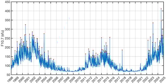
Figure 8.
Solar radio flux F10.7 from 1998 to 2024. The red points indicate the selected 88 local maxima of strong enhancements of F10.7. These time points are taken as timing marks for the epoch time of the composite analysis.
3.2. Results of the Composite Analysis
The composites of F10.7 and TEC for the 88 events are shown in Figure 9. It is strange that the spike in F10.7 at epoch time 0 induces no clear spike in global mean TEC. For each IGS TEC map, a global mean TEC value is derived by the area-weighted averaging of the zonal means. The zonal means are weighted by a factor where is the latitude.
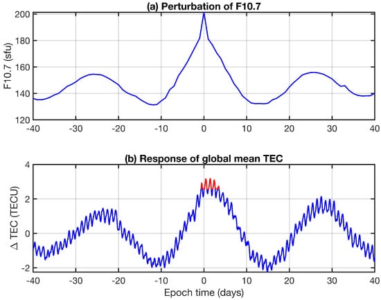
Figure 9.
Composites of the perturbation of F10.7 (a) and the response in global mean TEC (b). 88 events from 1998 to 2024. Line part in red color is used for determination of the time delay of the TEC response.
For the TEC composite, we removed all variations with periods larger than a half year by means of high pass filtering. Diurnal variations are included in the composite of TEC and are obviously present in Figure 9b. This indicates that a stronger response of TEC happens if the solar EUV enhancement occurs at a certain universal time. If the centre of mass is computed for all TEC values greater than TECmax (red values in Figure 9b), then a time lag of 1.4 days is obtained for the TEC response to solar EUV enhancements. However, the time lag of the TEC response is not well defined since there is no clear spike in TEC.
It has been reported that the time lag of TEC with respect to the solar EUV variation is often extended by geomagnetic activity [3]. In order to quantify the TEC response to geomagnetic storms, we calculated the composite of 389 events with Dst nT. The mean perturbation of Dst is shown in Figure 10a with a sharp negative spike at epoch time 0, indicating the end of the main phase of the geomagnetic storm and the beginning of the recovery phase. Again, we high-pass-filtered the Dst series to remove variations with periods greater than half a year. The diurnal variations are included in all composites. At high latitudes (magnetic latitude degrees) in Figure 10b in the Southern Hemisphere, one can see that a contribution of the diurnal variation is present in the TEC composite (red line). We noticed that the diurnal variation in the composite becomes stronger for extreme ionospheric storms. This may indicate a coupling between the storm’s main phase and universal time.
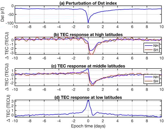
Figure 10.
Composites of the geomagnetic storm time index Dst (a) and the corresponding response in TEC at (b) high latitudes (absolute value of magnetic latitude greater than 60°), (c) middle magnetic latitudes (30 to 60 degrees in NH and SH), and (d) low magnetic latitudes (absolute value less than 30°).
At high latitudes in Figure 10b, a decrease of TEC is present about 0.5 days after the main phase. The TEC decrease is a negative storm effect, which is due to the transport of molecules to upper altitudes. Since molecular ions have a faster recombination rate than atomic ions, the electron density and TEC decrease when the ratio of O to N2 decreases. The TEC decrease is more than 3 TECU in the Southern Hemisphere. At middle magnetic latitudes (30 to 60 degrees in the Northern and Southern Hemispheres), a TEC decrease occurs about 0.6 days after the end of the main phase of the storm. The TEC decrease is more than 2 TECU. In the Northern Hemisphere, a positive storm effect (TEC increase) is present before epoch time 0. This can be due to vertical plasma transport, e.g., induced by prompt penetration electric fields (PPEFs; associated with the geomagnetic storm). At low magnetic latitudes (), a clear TEC increase of about 3 TECU occurs at epoch time 0. This positive ionospheric storm effect is associated with electrodynamic lifting of the plasma due to the storm-induced electric fields. The plasma is lifted to higher altitudes where the recombination rate is smaller. Thus, a TEC increase can be observed at low latitudes. The composite analysis showed that geomagnetic storms can induce average TEC changes of several TECU. Though the correlation between solar EUV variation and geomagnetic storms is small, it cannot be excluded that the correlation results between the 27-day oscillations of solar EUV and TEC are partly disturbed by geomagnetic activity.
4. Discussion
The 26-years long time series of TEC from IGS is valuable for determining the time delay between the 27-day oscillations of solar EUV (as represented by the proxies F10.7 and the MgII index) and the ionospheric TEC. Past observations and cross-correlation indicated that the TEC response can be delayed by 0 to 4 days [3]. There is a tendency that most observations indicate a time delay of 1 to 2 days [4]. However, simulations and observations by the CHAMP satellite favoured time delays of about 0.5 to 1 day. The present study shows that the time delay varies from 0.7 to 2.5 days depending on latitude and hemisphere. The global average of the time delay is 1.3 days for correlation with F10.7 and 1.1 days for correlation with the MgII index from SORCE. These results show that at some locations, the time delay is less than 1 day, as indicated by [3]. The global averages of the time delays (1.1 to 1.3 days) of the present study are in agreement with the observational study of [4]. A smaller time delay of about 1 day was reported by [12] for the 27-day variations of solar EUV and global mean TEC while a time delay of 2 days was reported by [1] for global mean TEC.
It is an open question why at some locations time delays of up to 2.1 (MgII) to 2.5 days (F10.7) can be reached. The simulations of [3] also showed an increase in the time delay with latitude and possible reasons such as solar zenith angle change, geomagnetic activity, and change in thermospheric circulation and O/N2 ratio were considered. In agreement with the observations by [5], we observed that the time delay is larger in the Southern Hemisphere than in the Northern Hemisphere. While Lee et al. reported an increase in the time delay by 1 day in the Southern Hemisphere, the present study finds that the time delay in the Southern Hemisphere is about 0.3 to 0.4 days greater than in the Northern Hemisphere. The simulations of [3] show a weaker asymmetry of the time delay in the hemispheres but with 0.1–0.2 days more time delay in the Southern Hemisphere (Figure 6e in [3]). However, Ren et al. [3] did not discuss this small difference of the time delays in the two hemispheres. In the present study, the interhemispheric asymmetry is particularly strong in the American longitude sector and the Asian–Australian sector (Figure 3). In both sectors, there are enough GNSS receivers in both hemispheres to ensure reliable TEC estimations. Thus, it would be worth considering an understanding of the observed asymmetry effect. One reason could be that geomagnetic activity effects are stronger in the Southern Hemisphere than in the Northern Hemisphere. Han et al. [13] found that large-scale travelling ionospheric disturbances were stronger in the Southern Hemisphere than in the Northern Hemisphere during the geomagnetic superstorm of May 2024. They also reported that during the geomagnetic storm, the O/N2 ratio in the Asian–Australian sector increased significantly, intensifying the hemispherical disparities, while the American sector exhibited a weaker asymmetry.
In agreement with past observational studies, we find that the correlation coefficient of TEC with F10.7 is a bit weaker than for TEC with the MgII index. This confirms the statement that the MgII index is a better proxy for solar EUV variations than F10.7 [14]. However, the MgII index series of SORCE is limited in time and also has a data gap. In spite of this, we took the SORCE series since the universal times of the MgII data are clearly given for SORCE and the time resolution is about 1.3 h. The hours of the universal times of the MgII composite of the University of Bremen are not or somehow unclearly documented in the daily values at https://www.iup.uni-bremen.de/UVSAT/data/ (accessed on 1 December 2025). However, we observed a time delay of 1.2 days for the MgII composite of the University of Bremen, which is close to the time delay of 1.1 days for the SORCE data. The correlation coefficient is 0.87 for TEC and Bremen data, which is a bit greater than for SORCE (0.85).
A second aim of the present study is the characterisation of the 27-day oscillation in TEC. We show that the amplitude can vary between 1 and 8 TECU. This variation can happen within half a year. The absolute variation of the TEC amplitude is largest at low latitudes. The mean amplitude of the 27-day oscillation is between 0.5 and 3 TECU over the globe with maxima at low geomagnetic latitudes at the place of the EIA. The amplitude is larger over Asia and Pacific ocean and a bit smaller above Africa and the Atlantic ocean. The relative mean amplitude of the 27-day oscillation in TEC is largest at high latitudes where it reaches mean values of up to 10% in both polar regions. To our limited knowledge, there are no reports in the literature yet about these characteristics of the 27-day oscillation in TEC.
Finally, we performed a composite analysis in order to study the TEC response with respect to solar EUV enhancements and to geomagnetic storms. The mean TEC response (Figure 9) is rather broad and relatively small (<3 TECU) with respect to the large spike in F10.7. With some effort, we can identify a time delay of 1.4 days for the TEC response but this value is not well defined because of the broad peak in TEC. Simulations of the TEC response to large spikes in F10.7 are not present in the literature. At the moment, one can only speculate that there are ionospheric–thermospheric processes which suppress a strong reaction of TEC to a strong solar EUV peak (from 140 to 200 sfu).
In order to quantify the mean TEC response with respect to geomagnetic storms, composite analysis was performed. Figure 10 shows that the TEC response can range from TECU (low magnetic latitudes) to TECU (high and middle magnetic latitudes). The positive TEC response at low latitudes is due to the prompt penetration electric field (PPEF), which is induced by the solar wind perturbation during the main phase of the geomagnetic storm. Buonsanto [15] divided ionospheric storms into positive storms and negative storms. The positive TEC change can be due to the upwelling of the ionospheric plasma to higher altitudes where the recombination rate is smaller. The negative TEC change can be due to a change in the O/N2 ratio, for example, when molecule-rich air from the lower thermosphere is transported into the middle and upper thermosphere. TEC will decrease in this case since the recombination is much faster for molecular ions than for atomic ions [16]. An extended composite analysis of the TEC response was performed by [17] who separated the dataset for seasons and degree of the geomagnetic storm.
Since the magnitude of the TEC response to geomagnetic storms is of the same order as those for solar EUV enhancements, it cannot be excluded that geomagnetic activity sometimes affects the correlation results of the solar EUV and TEC series. The correlation between solar EUV and geomagnetic activity is small but there is a relation between solar flares and solar wind speed. The solar wind speed near the Earth peaks about 2.5 days after the solar X-ray burst [18], and the solar wind speed closely correlates with geomagnetic activity.
5. Conclusions
We found time delays between TEC and the solar EUV proxy range from 0.7 to 2.5 days. The global average of the time delay was between 1.1 days (SORCE) and 1.3 days (F10.7). The time delay in the Southern Hemisphere was about 0.3 to 0.4 days longer than in the Northern Hemisphere. This agrees qualitatively with a former study by [5]. The reason of this hemispheric asymmetry of the TEC response is not clear yet. The simulation study by [3] shows a smaller difference between the time delays in both hemispheres (Figure 6e in [3]) but also with a greater time delay in the Southern Hemisphere. However, Ren et al. [3] did not discuss this effect.
The present study also shows the mean characteristics and the variability of the 27-day oscillation in TEC as a function of latitude and longitude. The mean amplitude of the 27-day oscillation is between 0.5 and 3 TECU over the globe with maxima at low geomagnetic latitudes at the place of the EIA. The relative mean amplitude of the 27-day oscillation in TEC reaches highest values of up to 10% in both polar regions.
The composite analysis provided the surprising result that a F10.7 peak of about 60 sfu just induces a broad TEC peak of about 3 TECU. The magnitude of this TEC perturbation is comparable to the TEC response to geomagnetic storms, but in the case of geomagnetic storms, the induced TEC peaks are much sharper.
Author Contributions
Conceptualisation and data curation, K.H. and G.M.; methodology, K.H.; software, K.H. and G.M.; formal analysis, K.H. and G.M.; writing—original draft preparation, K.H.; writing—review and editing, K.H. and G.M. All authors have read and agreed to the published version of the manuscript.
Funding
Open access funding was provided by the University of Bern.
Institutional Review Board Statement
Not applicable.
Informed Consent Statement
Not applicable.
Data Availability Statement
The TEC maps of the IGS are available at CDDIS, NASA’s archive of space geodesy data (https://cddis.nasa.gov/ (accessed on 1 December 2025)). The IGS is calculating these TEC maps [7]. The F10.7 and Dst data are provided by NASA’s Omniweb (https://omniweb.gsfc.nasa.gov/ (accessed on 1 December 2025). The MgII index of SORCE is distributed at https://lasp.colorado.edu/lisird/data/sorce_mg_index (accessed on 1 December 2025).
Acknowledgments
The International GNSS Service (IGS), NASA’s Omniweb, the Dominion Radio Astrophysical Observatory, University of Bremen and the SORCE mission are thanked for measurements and data. We thank the reviewers and the editor for their work in correcting and improving the manuscript. Open access funding was provided by the University of Bern.
Conflicts of Interest
The authors declare no conflicts of interest.
References
- Afraimovich, E.L.; Astafyeva, E.I.; Oinats, A.V.; Yasukevich, Y.V.; Zhivetiev, I.V. Global electron content: A new conception to track solar activity. Ann. Geophys. 2008, 26, 335–344. [Google Scholar] [CrossRef]
- Lean, J.L.; Meier, R.R.; Picone, J.M.; Sassi, F.; Emmert, J.T.; Richards, P.G. Ionospheric total electron content: Spatial patterns of variability. J. Geophys. Res. Space Phys. 2016, 121, 10367–10402. [Google Scholar] [CrossRef]
- Ren, D.; Lei, J.; Wang, W.; Burns, A.; Luan, X.; Dou, X. Does the Peak Response of the Ionospheric F2 Region Plasma Lag the Peak of 27-Day Solar Flux Variation by Multiple Days? J. Geophys. Res. Space Phys. 2018, 123, 7906–7916. [Google Scholar] [CrossRef]
- Schmölter, E.; Berdermann, J.; Codrescu, M. The Delayed Ionospheric Response to the 27-day Solar Rotation Period Analyzed With GOLD and IGS TEC Data. J. Geophys. Res. Space Phys. 2021, 126, e2020JA028861. [Google Scholar] [CrossRef]
- Lee, C.K.; Han, S.C.; Bilitza, D.; Seo, K.W. Global characteristics of the correlation and time lag between solar and ionospheric parameters in the 27-day period. J. Atmos. Sol.-Terr. Phys. 2012, 77, 219–224. [Google Scholar] [CrossRef]
- Ren, D.; Lei, J.; Wang, W.; Burns, A.; Luan, X.; Dou, X. Different Peak Response Time of Daytime Thermospheric Neutral Species to the 27-Day Solar EUV Flux Variations. J. Geophys. Res. Space Phys. 2020, 125, e2020JA027840. [Google Scholar] [CrossRef]
- Hernández-Pajares, M.; Juan, J.M.; Sanz, J.; Orus, R.; Garcia-Rigo, A.; Feltens, J.; Komjathy, A.; Schaer, S.C.; Krankowski, A. The IGS VTEC maps: A reliable source of ionospheric information since 1998. J. Geod. 2009, 83, 263–275. [Google Scholar] [CrossRef]
- Natali, M.P.; Urutti, A.; Castaño, J.M.; Zossi, B.S.; Duran, T.; Meza, A.; Elias, A.G. Long Term Global Ionospheric Total Electron Content Trend Analysis. Geophys. Res. Lett. 2024, 51, e2024GL112248. [Google Scholar] [CrossRef]
- Tapping, K.F. The 10.7 cm solar radio flux (F10.7). Space Weather 2013, 11, 394–406. [Google Scholar] [CrossRef]
- Snow, M.; Machol, J.; Viereck, R.; Woods, T.; Weber, M.; Woodraska, D.; Elliott, J. A Revised Magnesium II Core-to-Wing Ratio From SORCE SOLSTICE. Earth Space Sci. 2019, 6, 2106–2114. [Google Scholar] [CrossRef]
- Studer, S.; Hocke, K.; Kämpfer, N. Intraseasonal oscillations of stratospheric ozone above Switzerland. J. Atmos. Sol.-Terr. Phys. 2012, 74, 189–198. [Google Scholar] [CrossRef]
- Jacobi, C.; Jakowski, N.; Schmidtke, G.; Woods, T.N. Delayed response of the global total electron content to solar EUV variations. Adv. Radio Sci. 2016, 14, 175–180. [Google Scholar] [CrossRef]
- Han, T.; Le, H.; Yang, Y.; Li, W.; Sun, W.; Ma, H.; Zhou, Y.; Liu, B.; Du, R.; Liu, L.; et al. Characteristics of Large-Scale Traveling Ionospheric Disturbances During the 10 May 2024 Geomagnetic Storm. Space Weather 2025, 23, e2024SW004283. [Google Scholar] [CrossRef]
- Viereck, R.; Puga, L.; McMullin, D.; Judge, D.; Weber, M.; Tobiska, W.K. The Mg II index: A proxy for solar EUV. Geophys. Res. Lett. 2001, 28, 1343–1346. [Google Scholar] [CrossRef]
- Buonsanto, M.J. Ionospheric Storms—A Review. Space Sci. Rev. 1999, 88, 563–601. [Google Scholar] [CrossRef]
- Hargreaves, J.K. The Solar-Terrestrial Environment: An Introduction to Geospace-the Science of the Terrestrial Upper Atmosphere, Ionosphere, and Magnetosphere; Cambridge Atmospheric and Space Science Series; Cambridge University Press: Cambridge, UK, 1992. [Google Scholar] [CrossRef]
- Shinbori, A.; Otsuka, Y.; Sori, T.; Tsugawa, T.; Nishioka, M. Statistical Behavior of Large-Scale Ionospheric Disturbances From High Latitudes to Mid-Latitudes During Geomagnetic Storms Using 20-yr GNSS-TEC Data: Dependence on Season and Storm Intensity. J. Geophys. Res. Space Phys. 2022, 127, e2021JA029687. [Google Scholar] [CrossRef]
- Hocke, K. Oscillations of global mean TEC. J. Geophys. Res. Space Phys. 2008, 113. [Google Scholar] [CrossRef]
Disclaimer/Publisher’s Note: The statements, opinions and data contained in all publications are solely those of the individual author(s) and contributor(s) and not of MDPI and/or the editor(s). MDPI and/or the editor(s) disclaim responsibility for any injury to people or property resulting from any ideas, methods, instructions or products referred to in the content. |
© 2025 by the authors. Licensee MDPI, Basel, Switzerland. This article is an open access article distributed under the terms and conditions of the Creative Commons Attribution (CC BY) license (https://creativecommons.org/licenses/by/4.0/).