Abstract
Operational ensemble numerical weather prediction models are typically underspread near the land surface, with the Australian Bureau of Meteorology’s (BoM) global system being a typical example. In this study, land surface fraction values, representing the estimated proportions of various land cover types, are perturbed with the aim of increasing the ensemble spread at the surface. The perturbations are achieved by multiplying the existing land surface fraction estimates by spatially correlated random error structures that represent the uncertainties in these estimates. The methodology was trialed over a 75-day period during the Australian summer of 2017–2018 when both perturbed and unperturbed forecasting cycling experiments were run. The results showed that land surface fraction perturbations increased surface temperature, sensible heat flux, and latent heat flux ensemble spread significantly, especially in the tropics and over the Australian region. The screen-level temperature ensemble spread also increased, albeit by a relatively smaller magnitude compared to the surface temperature ensemble spread. Root-mean square error values—as measured relative to reanalysis data—were also found to be smaller in the perturbed runs, leading to significantly improved spread-to-skill ratio values.
1. Introduction
Ensemble numerical weather prediction models aim to quantify forecast uncertainties due to uncertainties in initial conditions, model parameters, and other model forcings such as sea surface temperatures and ancillaries. They accomplish this by running multiple simulations with initial conditions and parameter values sampled from these uncertainties [1]. Ensemble model forecasts provide improved guidance for end users in the form of probabilistic forecasting products that can be used for purposes such as risk management [2]. Short-range ensemble forecasts are also used by deterministic models to improve the characterization of error statistics for data assimilation [3,4,5,6].
Two key metrics in ensemble forecasting are ensemble skill and spread. Ensemble skill is a measure of the mean forecast error, while spread is a measure of the variability within the ensemble. Ideally, the spread–skill ratio in an ensemble forecast should be close to one [7,8,9,10,11,12], with some allowance made for uncertainty in the reference analyses. However, in practice, many ensemble forecasting systems are underspread [13,14]. Ensemble forecasts that are underspread have spread–skill ratios significantly less than one, meaning that the spread is much smaller than the mean forecasting error. This implies that the ensemble is unable to capture the full extent of the forecasting errors; in other words, the forecast is too confident. This problem is particularly acute at and near the surface of many atmospheric ensemble models [15,16,17,18]. This issue is likely related to the lack of variability within the land surface schemes that are used to represent the fluxes at the surface [19,20,21,22].
Figure 1 shows the spread–skill ratio of temperature at three vertical levels (500 hPa, 850 hPa, and the surface) in the Australian Bureau of Meteorology’s operational Australian Community Climate and Earth System Simulator Global Ensemble (ACCESS-GE) model [23] for the period between 16 and 31 January 2021. The ensemble underspread problem is shown clearly in this figure with values of the spread–skill ratio below 1 over all levels and forecast lead times. The spread–skill ratio is greatest for the mid-atmosphere (although below one) and drops through the lower atmosphere to the surface, most likely due to the lack of spread in modeled surface processes as alluded to above. The spread–skill ratios do, however, increase with lead time as ensemble members increasingly diverge due to the intrinsic nonlinearity of atmospheric motions.
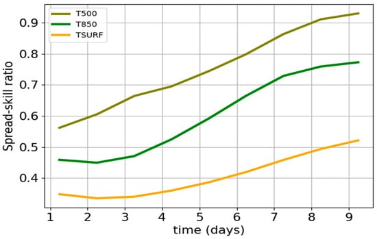
Figure 1.
Spread–skill ratio of temperature at three different heights (TSURF for surface temperature, T500 for 500 hPa pressure level, and T850 for 850 hPa pressure level) as obtained from the operational ACCESS-GE ensemble model for forecasting cycles averaged over the period 16 January–31 January 2021.
Previous studies have focused on a variety of strategies to address the surface underspread problem. Using regional ensemble models, Lavaysse et al. [19] and Bouttier et al. [20] perturbed several surface parameters such as vegetation fraction, leaf-area index, and albedo, as well as fields such as soil moisture and sea surface temperature. They used multiplicative perturbations for most parameters, although additive perturbations were used for some fields, such as sea surface temperature. They found significantly increased spread and skill in several near-surface fields such as screen-level temperature, particularly when perturbing soil moisture, albedo, leaf-area index, and sea surface temperature. However, Gehne et al. [21], using a global ensemble system, only reported “modest” increases in screen-level temperature skill when perturbing soil fields and various surface parameters such as roughness lengths, hydraulic conductivity, stomatal resistance, vegetation fraction, and albedo. They hypothesized that the low spread–skill ratio at the surface is caused more by temperature biases (resulting in large mean errors) rather than a lack of spread at the surface. Draper [22], on the other hand, using the United States National Centers for Environmental Prediction (NCEP)’s operational Global Ensemble Forecasting System (GEFS), found that vegetation fraction perturbations yield the most realistic impact on screen-level temperature spread compared to directly perturbing soil fields. This effect was conjectured as being caused by vegetation fraction perturbations directly affecting the fluxes between the land surface and the atmosphere, creating physically consistent perturbations in both components.
Given the mixed results obtained in previous studies, this study re-examines the effects of imposing surface perturbations with a focus on improving the Bureau’s global ensemble model, ACCESS-GE. Motivated by Draper’s results [22], only the land surface fractions, including both vegetation and non-vegetation fractions such as bare soil fractions, are perturbed herein. These fractions are multiplicatively perturbed with spatially correlated random error structures as described further in Section 2. In Section 3, the results obtained from the perturbed run are verified against ERA5 reanalysis data for selected surface fields and compared to a control run without surface perturbations. Section 4 contains a summary and discussion of the results, and Section 5 is the conclusion.
2. Materials and Methods
2.1. Model Description
A research version of the Bureau’s operational global ensemble model, ACCESS-GE, was used to perform the experiments in this study. This version of ACCESS-GE was run at a coarser resolution (about 60 km in the midlatitudes) compared to the operational version (about 30 km in the midlatitudes) and 70 vertical levels. The ACCESS-GE ensemble is centered on analyses of a higher resolution deterministic model, ACCESS-G, which, in the current study, was run at a resolution of about 40 km in the midlatitudes (compared to 12 km in the operational version). ACCESS-G3/GE3 is based on the UK Met Office GA6/GL6 atmosphere/land model configurations [24].
The number of members in the ensemble was 18, which is the same as in the operational version. The ACCESS-GE control member (Member 0) is initialized from a lower-resolution (~60 km) version of the ACCESS-G analysis. This analysis is obtained from a Hybrid 4DVar data assimilation scheme [3]. The Hybrid 4DVar scheme combines the error estimates obtained from the ensemble and climatology to generate the covariance matrix that is needed to create the analysis. Each component of the covariance matrix is given a weight that is determined empirically based on the forecasting skill of the ensuing system. In ACCESS-G, the ensembles contribute 30% to the hybrid error covariance matrix, while climatology provides the remaining 70%. Observations that are used include aircraft, radiosonde, and various surface and satellite observations. Perturbed members are initialized using the Local Ensemble Transform Kalman Filter data assimilation (LETKF) scheme [25,26]. The LETKF uses a transform matrix to generate ensemble initial conditions; the transform matrix is computed from a set of observations that are locally bound to mitigate spurious long-range correlations arising from an insufficient number of ensemble members. In ACCESS-GE, the bounding radius defining the length scale at which long-range correlations are ignored is about 5000 km [27]. The perturbations generated by LETKF need to be inflated because, as they currently stand, they tend to underestimate observed error growth. The inflation is computed by an adaptive scheme that is based on observed error growth rates from previous cycles.
Models run at coarse resolutions, such as ACCESS-GE (~60 km in this study), require parameterization schemes to account for unresolved processes such as convection, which occur at much smaller scales (<<10 km) [28]. ACCESS-G/GE employs a mass flux convection parameterization scheme based on Gregory and Rowntree [29] with various extensions to include down draughts [30] and convective momentum transport. Such parameterization schemes are inevitably associated with significant uncertainties, and therefore, ensemble members in ACCESS-GE are randomly perturbed at every model timestep to account for these uncertainties [31,32].
ACCESS-GE uses Sea Surface Temperatures (SSTs) to provide initial conditions over oceans. In this study, SSTs from the UK Met Office Operational SST and Sea-Ice Analysis (OSTIA) system [33] were used. Perturbations are also added to the SSTs to account for uncertainties, and these are different for each ensemble member [34]. Over land, the Joint UK Land Environment Simulator (JULES) [35] is used to model land surface processes. Soil temperature and moisture perturbations [34] are added to ensemble members to model uncertainties in the latest surface analysis obtained from ACCESS-G. This analysis is computed using the Simplified Extended Kalman Filter [36] data assimilation scheme to optimally combine JULES model outputs with surface and near-surface observations [37]. JULES uses nine land cover types to model surface fluxes, namely five vegetation cover types (broadleaf trees, needleleaf trees, C3 grass, C4 grass, and shrubs) and four non-vegetation cover types (urban, inland water, bare soil, and ice). Each land cover type describes a “tile” within the model with different surface fluxes, temperatures, and other relevant parameters. The net surface flux and temperature are therefore determined by the sum of the contributions from each land cover tile. In the operational version of ACCESS-GE and in the control experiment in this study, these land cover type fractions (or tile fractions) are treated as precise parameters and are therefore the same for each ensemble member. In reality, there is considerable uncertainty related to these fractions. They are based on International Geosphere-Biosphere Programme (IGBP) maps [38], which have various sources of uncertainty [39]. One source of uncertainty, for example, is the conversion from the 17 IGBP land cover types to the 9 cover types used in JULES, which is performed using look-up tables [40]. Additionally, vegetation fractions obtained from different maps, such as from the European Space Agency Climate Change Initiative (CCI) [41], can have significant differences compared to fractions from IGBP (see, for example, Figure 2 of Menon et al. [42]), which further illustrates the uncertainty associated with these ancillaries.
2.2. Land Surface Fraction Perturbations
As alluded to above, there is considerable uncertainty associated with the land surface fraction parameters, especially the vegetation cover types, and therefore it is of interest to understand the effect of perturbing these parameters. Multiplicative perturbations are used in this study as follows. Let be the unperturbed fraction for land type at the location with latitude and longitude . Then, the perturbed land surface fraction for ensemble member is calculated as
Here is a normalization factor that ensures that the perturbed fractions summed over all land surface types equal 1 and
is a coherent (spatially correlated) random scaling factor; (*) is a Gaussian filtering operation at the location (; and is a vector field of uncorrelated random scaling factors at all grid points in the domain. The uncorrelated scaling factors are obtained from the vector field of uncorrelated random numbers that are uniformly distributed in the range by the operation , which is a form of logarithmic sampling as further discussed in Appendix A; is treated as a tunable parameter and determines the amplitude of the random numbers . The index is a random selection from the land surface fraction types Gaussian filtering of the random perturbations is performed to create coherent (smoothed) error structures as shown in Equation (2). It is not clear, a priori, whether the degree of smoothing—if any—is required, so the degree of smoothing (i.e., the correlation length scale of the error structure) is treated as another tunable parameter in this study. Figure 2a shows an example of the unperturbed land fraction used in this study, namely the broadleaf tree vegetation fraction. Figure 2b shows a single realization of the corresponding perturbed land surface fraction with smoothing length scale corresponding to two grid lengths. The choice of multiplicative perturbations in this study was partly motivated by the observation that tile fractions close to 0 and 1 generally have the least uncertainty, and intermediate values are more uncertain [21]. For example, regions such as Antarctica, which are clearly covered by ice, have ice fractions of 1 and will not be perturbed by the scheme. The multiplicative perturbations in Equation (1) possess this desired property since there will be no perturbations when for land surface type ; that is, in that case. When , on the other hand, all other land surface types with different will have since fractions sum to one. Hence, the normalization factor and Equation (1) will then precisely yield , so tile fractions of 1 will not get perturbed either. The perturbed fractions used by Draper [22] also have this property, which in their case is accomplished by a scaling factor applied to the perturbations (their Equation (2)) designed to yield zero values when the tile fractions are 0 and 1.
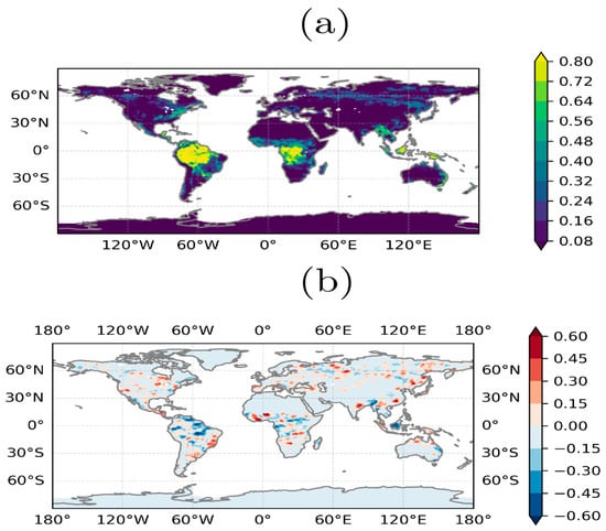
Figure 2.
(a) Broadleaf tree vegetation type base fraction and (b) difference between broadleaf tree perturbed vegetation fraction and base fraction.
2.3. Parameter Sensitivity Study
An initial parameter sensitivity study was conducted to determine suitable parameter values. The trial period for these ACCESS-GE runs was from 1 December 2017 to 20 December 2017. During this period, ACCESS-GE forecasts out to 192 h (8 days) lead time were produced every 6 h (at 0000Z, 0600Z, 1200Z, and 1800Z) by assimilating observations over a 6 h window centered at these base times, as is the practice operationally. These are referred to as forecasting cycles thereafter in this paper. The parameters varied were the random perturbation amplitude, , and the error structure correlation length scale, . These parameter values are shown in Table 1. A control ACCESS-GE experiment without land surface perturbations was also run to assess the effect of the perturbations in addition to the 12 experiments listed in Table 1.

Table 1.
Values of used to create random land surface fraction perturbations for different correlation length scales as described in Section 2.2.
Figure 3a shows the average screen-temperature spread difference percentage (relative to the control run) obtained for each experiment as a function of for three different smoothing length scales, namely, no smoothing ( km), moderate smoothing km), and large smoothing ( km). This plot shows that, as expected, the ensemble spread increases with increasing . The spread also appears to increase with increased smoothing. Because it is not completely clear how these parameters are related to the average perturbation size after normalization in Equation (1), the average perturbation size was determined for each experiment by computing the root mean square deviation of the perturbations, averaged over all land surface types. Figure 3b shows the spread percentage difference as a function of the average perturbation size. This shows that the spread increases with land surface fraction and average perturbation size, and that the rate of increase depends on the degree of smoothing. Without smoothing, the spread increases very slowly with increasing perturbation size, while with smoothing, the spread increases more rapidly. The increase in spread is approximately quadratic when smoothing is applied. With very high values (~5), numerical instability developed in the model runs after being run for several weeks, and so the smaller value (with large smoothing) was chosen as the target experiment in this study.
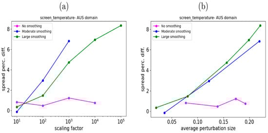
Figure 3.
(a) Spread percentage difference as a function of and (b) average perturbation size over the Australian domain.
2.4. Verification Method
ACCESS-GE control forecasts (with unperturbed land surface fractions) and experimental forecasts (with perturbed land surface fractions) were verified against ERA5 reanalysis data. ERA5 is a global reanalysis dataset of atmospheric climate variables on a regular grid at a resolution of approximately 30 km with 137 vertical levels from the surface up to approximately 80 km and a temporal frequency of 1 h. ERA5 uses the 4DVar data assimilation scheme to blend observations from over 200 satellite and conventional instruments with forecasts from ECMWF’s world-leading Integrating Forecasting System (IFS) over a 12 h window [43]. The following metrics were used to perform the verification: spread (computed as the square root of the spatial mean ensemble variance), root mean square error of the ensemble mean (RMSE), and spread–skill ratio (computed as the ratio of spread/RMSE). The focus of the verification was on surface and near-surface fields, namely surface temperature, screen-level temperature, sensible heat flux, and latent heat flux. The verification was performed at a resolution of 1.5° over land only and at lead times of 24 h, 48 h, 72 h, …, 192 h. The following regions were considered: global, tropics (i.e., between 23.5° N and 23.5° S), and Australia (longitudes 112–154° E, latitudes 10–40° S), the latter being of interest because of its importance to Bureau operations.
2.5. Trial Details
Extended ACCESS-GE control and experiment runs were performed from 1 December 2017 until 22 February 2018, corresponding to the Australian summer when the effect of land surface perturbations is expected to be maximal over the Australian continent due to increased solar insolation and leaf cover. In the control run, no land surface fraction perturbations were applied, while in the experiment, land surface perturbations with and km, as alluded to in Section 2.3, were used. Both the control and experiment were sampled for 75 days starting from 10 December 2017, and the output fields were verified against ERA5 data, the results of which are presented below.
3. Results
3.1. Global Domain Verification
Figure 4 shows the surface temperature, screen-level temperature, sensible heat flux, and latent heat flux spread–skill ratios for the unperturbed and perturbed runs as a function of lead time, as verified over the whole globe after averaging over all forecasting cycles in the 75-day trial. The surface temperature spread–skill ratio in the perturbed run is seen to increase slightly (by about 5% at short lead times), indicating a small improvement to the ensemble at the surface. However, the screen-level temperature spread–skill ratio improvement is much smaller compared to the surface and appears to be largely neutral overall. The surface flux spread–skill ratios do, however, appear to increase significantly because of the perturbations, indicating an improvement to the ensemble.
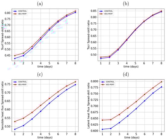
Figure 4.
Spread–skill ratios computed over the global domain for the unperturbed control run (blue) and perturbed run (red). Spread–skill ratios for four different fields are shown: (a) surface temperature, (b) screen-level temperature, (c) sensible heat flux, and (d) latent heat flux.
3.2. Tropical Domain Verification
Figure 5 shows the same plots as in Figure 4 but calculated over the tropics only. This figure reveals that the increases in spread–skill ratios are significantly larger in the tropics. The surface temperature spread–skill ratio increases by over 25% in this region, from about 0.4 to over 0.5. The screen-level temperature spread–skill ratio also increases in this region, albeit by a lesser margin (~15%). Surface flux spread–skill ratios are also improved. It should be noted that the spread–skill ratio increases are associated with both increased spread and reduced ensemble-mean errors. For example, for surface temperature, the ensemble spread increased by about 0.3 K, and the ensemble-mean RMSE reduced by about 0.05 K.
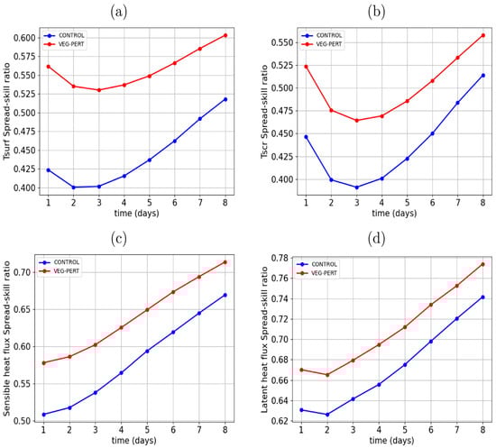
Figure 5.
Spread–skill ratios computed over the tropical domain for the unperturbed control run (blue) and perturbed run (red). Spread–skill ratios for four different fields are shown: (a) surface temperature, (b) screen-level temperature, (c) sensible heat flux, and (d) latent heat flux.
3.3. Australian Domain
Spread–skill ratios for selected surface fields were also calculated over Australia. The overall trends in the spread–skill ratios are similar to those calculated over the globe and tropics, and demonstrate improvements in all four surface fields considered, with magnitudes of improvements somewhere in between those obtained for the globe and those obtained for the tropics. For this region, the verification statistics were further subdivided according to the time of day. Since only forecasts at times 0000Z, 0600Z, 1200Z, and 1800Z were considered, the first two times were classified as ‘day’ and the last two times as ‘night’, which is accurate over most of Australia. Spread–skill ratios computed separately for these periods of the day are shown in Figure 6. It can be seen that spread–skill ratios for different surface fields increase during both day and night, albeit by different amounts. Surface temperature and latent heat improvements are greatest during the day. The sensible heat flux shows about the same level of improvement during the day and night. However, relative improvements for screen-level temperature are greatest during the night. Since the screen-level temperature is computed by interpolating the surface and lowest model level temperatures, this suggests that changes in surface temperature, such as those induced by land surface perturbations, influence the lower atmosphere more during the night.
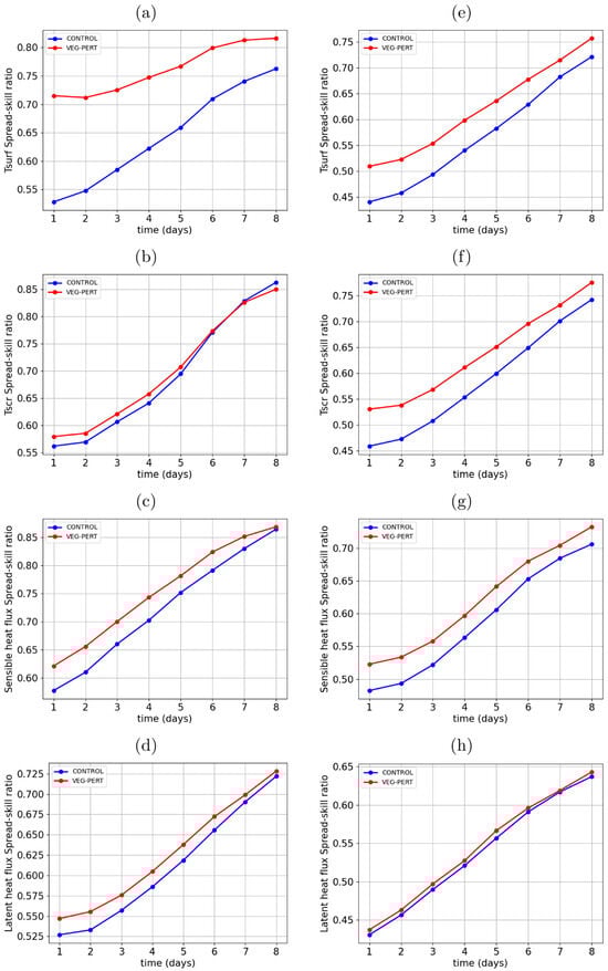
Figure 6.
Spread–skill ratios computed over the Australian domain for the unperturbed control run (blue) and perturbed run (red). Left panels (a–d) show spread–skill ratios for surface temperature, screen-level temperature, sensible heat flux, and latent heat flux, respectively, during the day, while right panels (e–h) show the same fields during the night.
Several observational studies have confirmed that surface temperatures are generally better correlated with screen-level temperatures during the night [44,45]. This effect also appears to be a robust feature of both the ACCESS-GE4 model and ERA5 reanalyses. We have confirmed that screen-level temperatures are better correlated with surface temperatures during the night compared to during the day in both ACCESS-GE and ERA5, even without surface perturbations in the former. Figure 7 demonstrates the diurnal variation of the mean pattern correlation between the surface and screen-level temperature as a function of lead time of all 0000Z basetimes during December 2017. This mean pattern correlation follows a cyclic pattern, with lows during the day and highs during the night over the Australian domain. The cyclic pattern is seen in both perturbed and unperturbed experiments. ERA5 reanalysis data also display this diurnal pattern.
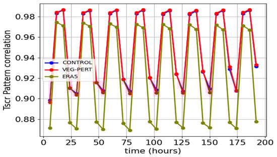
Figure 7.
Mean pattern correlation between surface and screen-level temperatures computed over the Australian domain as a function of lead time (in 6 h intervals) of all base 0000Z basetimes in December 2017. The plot demonstrates the diurnal variation of the pattern correlation between the surface and screen-level temperatures. Lead times of 24 h, 48 h, 72 h… as well as 6 h, 30 h, 54 h… occur during the day in this domain. Lead times of 12 h, 36 h, 60 h… and 18 h, 42 h, 66 h… occur during the night. Mean pattern correlations are shown for unperturbed ACCESS-GE ensemble mean (CONTROL), perturbed ACCESS-GE ensemble mean (VERG-PERT), and ERA5 reanalysis (ERA5).
Figure 8 shows the differences between 24 h perturbed and unperturbed surface and screen-level temperature ensemble standard deviation forecasts over the Australian domain during the 20171210T0000Z and 20171210T1200Z cycles, which are the first two cycles in the 75-day period used to verify the forecasts. The 20171210T0000Z + 24 h valid time occurs during the day in this domain, while the 20171210T1200Z + 24 h valid time occurs during the night. Land surface fraction perturbations are seen to increase surface and screen-level temperature ensemble spread during both day and night, albeit with differing amounts. The surface temperature ensemble spread increases by at least 2 K over most of the Australian continent during the day, as shown in Figure 8a. During the night [Figure 8b], the increase in spread is smaller in magnitude, except over north-central Australia. Screen-level temperature spread also increases, albeit by smaller amounts. Additionally, the increase in screen-level temperature spread is greater during the night [Figure 8d] compared to during the day [Figure 8c]. Surface temperature spread differences between day and night reflect higher surface temperature values during the day compared to the night due to differences in solar insolation. Differences in screen-level temperature spread also reflect different boundary layer processes during the day and night. During the night, the screen-level temperature is better correlated with the surface temperature compared to during the day, as shown in the pattern correlation values in Figure 7 and by visually comparing the patterns in Figure 8.
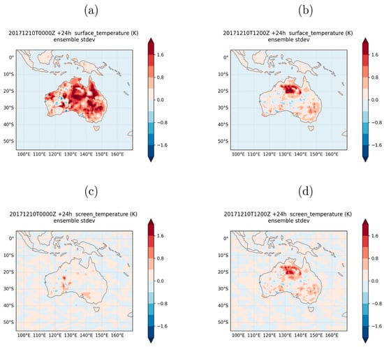
Figure 8.
Difference between perturbed and unperturbed ensemble standard deviations during the day panels (a,c) and night panels (b,d) over Australia. The top panels (a,b) show surface temperatures, while the bottom panels (c,d) show screen-level temperatures. The day and night forecasts are valid at 0000Z and 1200Z, respectively, on 2 December 2017 (in Coordinated Universal Time).
4. Discussion
In this study, a technique for perturbing land surface fraction parameters in an ensemble model (ACCESS-GE) was presented, and the results were evaluated against a control run without land surface perturbations during the Australian summer of 2017. The nine intrinsic tile fraction parameters were perturbed multiplicatively by a random number field and then normalized to generate a new set of tile fraction parameters for each ensemble member. A convenient feature of multiplicative perturbations is that tiles with fractions of 0 and 1 do not become perturbed, which is consistent with the observation that the greatest uncertainty occurs in tile fractions with intermediate values [21]. The perturbations were dependent on two free parameters, namely, the maximum amplitude and the correlation length scale of the random field. A sensitivity study was performed for the first 3 weeks of the trial period to understand the response of the system to different values of these parameters. It was found (not surprisingly) that larger maximum random amplitudes yielded greater model responses (i.e., bigger ensemble spread). However, numerical instabilities also developed in some of the larger amplitude runs, and so a maximum random amplitude value of 3 was chosen for the long 75-day trial to create a compromise between model response and numerical instability. It was also found that random fields with larger correlation length scales (120 km) yielded better model responses than uncorrelated random fields and random fields with smaller correlation length scales (60 km), hence the selection of the larger 120 km correlation length scale in the longer 75-day trial. It should be noted that Lavaysse et al. [19] employed even larger correlation length scales in their study, namely 500–1000 km. Correlation length scales that large were not trialed in this study, but given that the increase in spread between the runs with correlation length scales of 60 km and 120 km was relatively modest (see Figure 3b), it is not clear whether substantially increasing the length scale will be beneficial.
Selected surface field forecasts over land from the longer trial period of 75 days using perturbed tile fractions were verified against ERA5 reanalysis data and compared to forecasts from the corresponding control run with unperturbed tile fractions. Three verification domains were used, namely, global, tropical, and Australia. The results showed that the strongest model response to tile fraction perturbations occurred in the tropical domain. The Australia domain also demonstrated significant model response, but the overall global response to perturbations was relatively small, especially for the screen-level temperature field, which is an interpolation of surface and lowest atmospheric-level temperature fields. These patterns reflect seasonal variations in solar insolation and leaf coverage. The tropics are characterized by nearly constant solar insolation and significant leaf coverage throughout the year, which results in a stronger response to land surface fraction perturbations. During the December–February period, the southern hemisphere experiences significantly higher insolation and leaf production compared to the northern hemisphere, which explains the stronger response seen over Australia and the weaker global response patterns. The northern parts of Australia are also located in the tropics, which partly explains the significant response in this region. It is expected that during the Australian winter, the response over the southern parts of Australia would be weaker due to reduced solar insolation and leaf cover. It should be noted that these geographical patterns in model response to land surface perturbations are consistent with those found by Gehne et al. [21].
In all domains considered, there was an increase in surface temperature and (sensible and latent) heat flux spread when employing the surface perturbations. The ensemble-mean RMSE—as measured relative to ERA5 data—was also reduced, indicating better skill in the perturbed run (in agreement with the results of Lavaysse et al. [19]). The spread–skill ratio consequently increased at the surface, exceeding 25% in tropical regions, indicating better ensemble forecasting capability overall compared to not employing the surface perturbations. The screen-level temperature spread also increased, albeit by a smaller amount. Since screen-level temperature is an interpolation of surface and lower atmosphere temperature, this suggests that changes in screen-level spread were dominated by changes in surface spread rather than changes in the lower atmosphere spread. It is not clear why the increased surface flux spread was not propagated to the lower atmosphere to a greater extent within the ACCESS-GE model. Future work with convection-permitting regional models could help address this question; however, it should be noted that using a convection-permitting high-resolution model, Bouttier et al. [20] obtained broadly similar results to those obtained with coarser-resolution models, so it is not clear to what extent the model response would differ if surface perturbation were employed in a high-resolution model. The screen-level temperature spread increase in the tropics was about 0.3 K, which is comparable to the 0.4 K value reported by Gehne et al. [21], although in that study the increased spread was obtained by perturbing multiple land surface variables, not just the vegetation fraction.
The diurnal variation of the increased spread was also examined in the Australian domain. This revealed, as expected, bigger changes in surface temperature and flux spreads during the day compared to during the night, presumably due to differences in solar insolation. However, screen-level temperature spread changed more during the night than during the day. Further analysis was performed to understand the diurnal variation of the coupling between surface and lower-atmosphere temperatures by computing the pattern correlation between surface and screen-level temperatures. This revealed that the screen-level temperature is always better correlated with the surface temperature during the night than during the day. This cyclic pattern was seen not only in the perturbed and unperturbed ACCESS-GE models but also in the ERA5 reanalysis data. Hence, the greater response of the ACCESS-GE screen-level temperature to surface perturbations during the night compared to during the day could be explained by the intrinsically stronger coupling of the lower atmosphere to the surface during the night that is exhibited by the models. Increased screen-level temperature spread during the night compared to during the day was also reported by Gehne et al. [21] in the context of a different atmospheric model (GEFS), with perturbing vegetation fractions, which further suggests that it is a common feature of different atmospheric models that reflects the diurnal variation in the interaction between the surface and the lower atmosphere.
In agreement with the results of Lavaysse et al. [19], Gehne et al. [21], and Draper [22], the results obtained from this study demonstrate that perturbing land surface tile fractions is an effective way of ameliorating the ensemble underspread at and near the surface in ensemble numerical weather prediction models. The perturbations represent uncertainties in the estimation of the tile fractions. They also represent, to an extent, uncertainties due to unresolved physical processes in modeling surface fluxes of heat and moisture. Hence, in this study, a tuning approach was followed in specifying the amplitude and spatial structure of the perturbations rather than attempting to estimate the uncertainties directly. The perturbations were tuned to yield significant increases in ensemble spread while maintaining numerical stability. As alluded to above, however, the surface perturbations did not appear to significantly influence the lower atmosphere. Future studies should be focused on better understanding this phenomenon and finding solutions to allow greater model responses in the lower atmosphere to the surface perturbations.
5. Conclusions
Land surface tile fractions representing proportions of various vegetative and non-vegetative surfaces in the ACCESS-GE global ensemble model were perturbed using random multiplicative factors and the results compared to a control run without land surface perturbations during a 75-day trial in December–February 2017. The results showed that ensemble spread and spread-to-skill ratios of surface temperature and heat fluxes increased in the perturbed run, indicating improved ensemble quality, especially in the tropics and in the Australian region. Screen-level temperature spread and spread-to-skill ratios also increased, but by relatively smaller amounts compared to the surface.
Author Contributions
Conceptualization, M.J.Z., P.J.S., and I.D.; methodology, M.J.Z., P.J.S., and I.D.; software, M.J.Z.; validation, M.J.Z., P.J.S., and I.D.; formal analysis, M.J.Z., P.J.S., and I.D.; investigation, M.J.Z., P.J.S., and I.D.; resources, M.J.Z., P.J.S., and I.D.; data curation, M.J.Z.; writing—original draft preparation, M.J.Z., P.J.S., and I.D.; writing—review and editing, M.J.Z., P.J.S., and I.D.; visualization, M.J.Z. All authors have read and agreed to the published version of the manuscript.
Funding
This research received no external funding.
Institutional Review Board Statement
Not applicable.
Informed Consent Statement
Not applicable.
Data Availability Statement
Data are available upon request.
Acknowledgments
We would like to acknowledge Jin Lee, formerly of the Bureau of Meteorology, for building and maintaining the research version of the ACCESS-GE suite on the National Computing Infrastructure (NCI) facility on which the experiments reported herein were conducted. We would also like to acknowledge Craig H. Bishop, from the University of Melbourne, for suggesting experimentation with spatially correlated error structures. Chun-Hsu Su and Andrew Frost, from the Bureau of Meteorology, reviewed the manuscript and provided useful suggestions. This work was undertaken with the assistance of computational resources and services from NCI, which is supported by the Australian Government. NCI provides a replication of the ERA5 dataset used in this work. ERA5 is produced by ECMWF and distributed via Copernicus Climate Change Service (C3S).
Conflicts of Interest
The authors declare no conflicts of interest.
Abbreviations
The following abbreviations are used in this manuscript:
| NCI | National Computing Infrastructure |
| ACCESS | Australian Community Climate and Earth System Simulator |
| GE | Global ensemble |
Appendix A. Logarithmic Sampling
As alluded to in Section 2.2, a logarithmic sampling approach was used to generate the spatially uncorrelated scaling factors in Equation (2), where the index represents the land surface type and represents the ensemble member (i.e., a sample); the bold notation signifies that different scaling factors are computed at each grid point. To simplify the discussion in this section, consider a single grid point and land surface type and denote these scaling factors by . The motivation for the logarithmic approach was to ensure that the perturbed land surface fractions remain centered on the unperturbed land surface values derived from the IGBP dataset (see Section 2.1); this requires the values to be centered on 1. To accomplish this, values of need to be sampled as frequently as values of Since , this implies that the distribution must be skewed, with number of samples in the range [0, 1] roughly equal to the number of samples in the range [1, R], where R is the specified maximum value of the scaling factor, assumed to be greater than 1. To facilitate symmetric logarithmic sampling, a further restriction is imposed, namely that the sample range is [1/R, R] rather than [0, R], so that in logarithmic space, is in the range . Once is sampled, the scaling factors are obtained by inverting this relationship, namely .
Figure A1 shows the difference between these two sampling approaches when R = 2, using 1000 samples. Panel (a) shows the frequency distribution with uniform sampling (without transforming into logarithmic space). The frequency distribution is approximately uniform as expected, and values greater than 1.0 are sampled roughly twice as frequently as values less than 1.0. Should this sampling method be used, the ensemble would clearly be biased towards higher land surface fraction values. On the other hand, if the uniform sampling is performed in logarithmic space as in Panel (b), a different distribution emerges. This logarithmically sampled distribution is skewed towards values less than 1.0, and values less than 1.0 are sampled roughly at the same frequency as values greater than 1.0. That means the ensemble will roughly remain centered on the unperturbed value when using this sampling method.

Figure A1.
Frequencies of 1000 sampled scaling factor values in the range [0.5, 2.0] for (a) uniform sampling and (b) logarithmic sampling.
References
- Gneiting, T.; Raftery, A.E. Weather forecasting with ensemble methods. Science 2005, 310, 248–249. [Google Scholar] [CrossRef]
- Palmer, T.N. The economic value of ensemble forecasts as a tool for risk assessment: From days to decades. Q. J. R. Meteorol. Soc. 2002, 128, 747–774. [Google Scholar] [CrossRef]
- Clayton, A.; Lorenc, A.; Barker, D. Operational implementation of a hybrid ensemble/4D-Var global data assimilation system at the Met Office. Q. J. R. Meteorol. Soc. 2013, 139, 1445–1461. [Google Scholar] [CrossRef]
- Wang, X.; Parrish, D.; Kleist, D.; Whitaker, J. GSI 3DVar-based ensemble–variational hybrid data assimilation for NCEP Global Forecast System: Single-resolution experiments. Mon. Weather. Rev. 2013, 141, 4098–4117. [Google Scholar] [CrossRef]
- Kleist, D.T.; Ide, K. An OSSE-based evaluation of hybrid variational–ensemble data assimilation for the NCEP GFS. Part I: System description and 3D-hybrid results. Mon. Weather. Rev. 2015, 143, 433–451. [Google Scholar] [CrossRef]
- Buehner, M.; McTaggart-Cowan, B.A.R.; Charette, C.; Garand, L.; Heilliette, S.; Lapalme, E.; Laroche, S.; Macpherson, S.; Morneau, J.; Zadra, A. Implementation of deterministic weather forecasting systems based on ensemble–variational data assimilation at Environment Canada. Mon. Weather. Rev. 2015, 143, 2532–2559. [Google Scholar] [CrossRef]
- Palmer, T.; Buizza, R.; Hagedorn, R.; Lawrence, A.; Leutbecher, M.; Smith, L. Ensemble prediction: A pedagogical perspective. ECMWF Newsl. 2006, 106, 10–17. [Google Scholar]
- Leutbecher, M.; Palmer, T. Ensemble forecasting. J. Comput. Phys. 2008, 227, 3315–3539. [Google Scholar] [CrossRef]
- Fortin, V.; Abaza, M.; Anctil, F.; Turcotte, R. Why should ensemble spread match the RMSE of the ensemble mean? J. Hydrometeorol. 2014, 15, 1708–1713. [Google Scholar] [CrossRef]
- Haiden, T.; Janousek, M.; Vitart, F.; Bouallegue, Z.; Ferranti, L.; Prates, F.; Richardson, D. Evaluation of ECMWF Forecasts, Including the 2018 Upgrade; European Centre for Medium Range Weather Forecasts: Reading, UK, 2018. [Google Scholar]
- Rodwell, M.; Richardson, D.; Parsons, D.; Wernli, H. Flow-dependent reliability: A path to more skillful ensemble forecasts. Bull. Am. Meteorol. Soc. 2018, 99, 1015–1026. [Google Scholar] [CrossRef]
- Roberts, C.; Leutbacher, M. Unbiased calculation, evaluation, and calibration of ensemble forecast anomalies. Q. J. R. Meteorol. Soc. 2025, 151, e4993. [Google Scholar] [CrossRef]
- Buizza, R.; Barkmeijer, J.; Palmer, T.N.; Richardson, D.S. Current status and future developments of the ECMWF Ensemble Prediction System. Meteorol. Appl. 2000, 7, 163–175. [Google Scholar] [CrossRef]
- Palmer, T.N.; Shutts, G.J.; Hagedorn, R.; Doblas-Reyes, F.J.; Jung, T.; Leutbecher, M. Representing model uncertainty in weather and climate prediction. Annu. Rev. Earth Planet. Sci. 2005, 33, 163–193. [Google Scholar] [CrossRef]
- Mullen, S.L.; Buizza, R. Quantitative precipitation forecasts over the United States by the ECMWF ensemble prediction system. Mon. Weather. Rev. 2001, 129, 638–663. [Google Scholar] [CrossRef]
- Hamill, T.M.; Whitaker, J.S. Ensemble calibration of 500-hPa geopotential height and 850-hPa and 2-m temperatures using reforecasts. Mon. Weather. Rev. 2007, 135, 3273–3280. [Google Scholar] [CrossRef]
- Flowerdew, J.; Bowler, N.E. Improving the use of observations to calibrate ensemble spread. Q. J. R. Meteorol. Soc. 2011, 137, 467–482. [Google Scholar] [CrossRef]
- Flowerdew, J.; Bowler, N.E. On-line calibration of the vertical distribution of ensemble spread. Q. J. R. Meteorol. Soc. 2013, 139, 1863–1874. [Google Scholar] [CrossRef]
- Lavaysse, C.; Carrera, S.; Belair, N.; Gagnon, R.; Frenette, M.; Yau, M. Impact of surface parameter uncertainties within the Canadian Regional Ensemble Prediction System. Mon. Weather. Rev. 2013, 141, 1506–1526. [Google Scholar] [CrossRef]
- Bouttier, F.; Raynaud, L.; Nuissier, O.; Ménétrier, B. Sensitivity of the AROME ensemble to initial and surface perturbations during HyMeX. Q. J. R. Meteorol. Soc. 2016, 142, 390–403. [Google Scholar] [CrossRef]
- Gehne, M.; Hamill, T.; Bates, G.T.; Pegion, P.; Kolczynski, W. Land surface parameter and state perturbations in the Global Ensemble Forecast System. Mon. Weather. Rev. 2019, 147, 1319–1340. [Google Scholar] [CrossRef]
- Draper, C. Accounting for Land Model Uncertainty in Numerical Weather Prediction Ensemble Systems: Toward Ensemble-Based Coupled Land–Atmosphere Data Assimilation. J. Hydrometeorol. 2021, 22, 2089–2104. [Google Scholar]
- Bureau of Meteorology. APS3 Upgrade of the ACCESS-G/GE Numerical Weather Prediction System; Operations Bulletin Number 125; Bureau of Meteorology National Operational Centre: Melbourne, Australia, 2019.
- Walters, D.B.I.; Brooks, M.; Melvin, T.; Stratton, R.; Vosper, S.; Wells, H.; Williams, K.; Wood, N.; Allen, T.; Bushell, A. The Met Office unified model global atmosphere 6.0/6.1 and JULES global land 6.0/6.1 configurations. Geosci. Model Dev. 2017, 10, 1487–1520. [Google Scholar] [CrossRef]
- Bishop, C.; Etherton, B.; Majumdar, S. Adaptive sampling with the ensemble transform Kalman filter. Part I: Theoretical aspects. Mon. Weather. Rev. 2001, 129, 420–436. [Google Scholar] [CrossRef]
- Hunt, B.; Kostelich, E.; Szunyogh, I. Efficient data assimilation for spatiotemporal chaos: A local ensemble transform Kalman filter. Phys. D Nonlinear Phenom. 2007, 230, 112–126. [Google Scholar] [CrossRef]
- Zidikheri, M.J.; Steinle, P.J.; Xiao, Y.; Villardon, E.A. An objective evaluation of the Bureau’s ACCESS-GE4 global ensemble model. Aust. Bur. Meteorol. Melb. 2024, 137, 1717–1720. [Google Scholar]
- Yano, J.; Ziemiański, M.; Cullen, M.; Termonia, P.; Onvlee, J.; Bengtsson, L.; Carrassi, A.; Davy, R.; Deluca, A.; Gray, S.; et al. Scientific challenges of convective-scale numerical weather prediction. Bull. Am. Meteorol. Soc. 2018, 99, 699–710. [Google Scholar] [CrossRef]
- Gregory, D.; Rowntree, P.R. A mass flux convection scheme with representation of cloud ensemble characteristics and stability-dependent closure. Mon. Weather. Rev. 1990, 118, 1483–1506. [Google Scholar] [CrossRef]
- Gregory, D.; Allen, S. The effect of convective scale downdraughts upon NWP and climate simulations. In Proceedings of the 9th Conference on Numerical Weather Prediction, Denver, CO, USA, 14–18 October 1991; pp. 122–123. [Google Scholar]
- Bowler, N.; Arribas, A.; Mylne, K.; Robertson, K.; Beare, S. The MOGREPS short-range ensemble prediction system. Q. J. R. Meteorol. Soc. 2008, 134, 703–722. [Google Scholar] [CrossRef]
- Bowler, N.; Arribas, A.; Beare, S.; Mylne, K.; Shutts, G. The local ETKF and SKEB: Upgrades to the MOGREPS short-range ensemble prediction system. Q. J. R. Meteorol. Soc. 2009, 135, 767–776. [Google Scholar] [CrossRef]
- Donlon, C.; Martin, M.; Stark, J.; Roberts-Jones, J.; Fiedler, E.; Wimmer, W. The operational sea surface temperature and sea ice analysis (OSTIA) system. Remote Sens. Environ. 2012, 116, 140–158. [Google Scholar]
- Tennant, W.; Beare, S. New schemes to perturb sea-surface temperature and soil moisture content in MOGREPS. Q. J. R. Meteorol. Soc. 2013, 140, 1150–1160. [Google Scholar] [CrossRef]
- Best, M.; Pryor, M.; Clark, D.; Rooney, G.; Essery, R.; Ménard, C.; Edwards, J.; Hendry, M.; Porson, A.; Gedney, N.; et al. The Joint UK Land Environment Simulator (JULES), model description–Part 1: Energy and water fluxes. Geosci. Model Dev. 2011, 4, 677–699. [Google Scholar] [CrossRef]
- De Rosnay, P.; Drusch, M.; Vasiljevic, D.; Balsamo, G.; Albergel, C.; Isaksen, L. A simplified extended Kalman filter for the global operational soil moisture analysis at ECMWF. Q. J. R. Meteorol. Soc. 2013, 139, 1199–1213. [Google Scholar] [CrossRef]
- Gómez, B.; Charlton-Pérez, C.; Lewis, H.; Candy, B. The Met Office Operational Soil Moisture Analysis System. Remote Sens. 2020, 12, 3691. [Google Scholar] [CrossRef]
- Loveland, T.; Belward, A. The IGBP-DIS global 1km land cover data set, DISCover: First results. Int. J. Remote Sens. 1997, 18, 3289–3295. [Google Scholar] [CrossRef]
- Zhang, M.; Ma, M.; De Maeyer, P.; Kurban, A. Uncertainties in classification system conversion and an analysis of inconsistencies in global land cover products. ISPRS Int. J. Geo-Inf. 2017, 6, 112. [Google Scholar] [CrossRef]
- Wiltshire, A.; Rojas, M.D.; Edwards, J.; Gedney, N.; Harper, A.; Hartley, A.; Hendry, M.; Robertson, E.; Smout-Day, K. JULES-GL7: The Global Land configuration of the Joint UK Land Environment Simulator version 7.0 and 7.2. Geosci. Model Dev. 2020, 13, 483–505. [Google Scholar] [CrossRef]
- Poulter, B.; MacBean, N.; Hartley, A.; Khlystova, I.; Betts, A.O.R.; Bontemps, S.; Boettcher, M.; Brockmann, C.; Defourny, P.; Hagemann, S. Plant functional type classification for earth system models: Results from the European Space Agency’s Land Cover Climate Change Initiative. Geosci. Model Dev. 2015, 8, 2315–2328. [Google Scholar] [CrossRef]
- Menon, A.; Turner, A.; Volonte, A.; Taylor, C.; Webster, S.; Martin, G. The role of mid-tropospheric moistening and land-surface wetting in the progression of the 2016 Indian monsoon. Q. J. R. Meteorol. Soc. 2022, 148, 3033–3055. [Google Scholar] [CrossRef]
- Hersbach, H.; Coauthors, A. The ERA5 global reanalysis. Q. J. R. Meteorol. Soc. 2020, 146, 1999–2049. [Google Scholar] [CrossRef]
- Good, E. An in situ-based analysis of the relationship between land surface “skin” and screen-level air temperatures. J. Geophys. Res. Atmos. 2016, 121, 8801–8819. [Google Scholar] [CrossRef]
- Good, E.; Ghent, D.; Bulgin, C.; Remedios, J. A spatiotemporal analysis of the relationship between near-surface air temperature and satellite land surface temperatures using 17 years of data from the ATSR series. J. Geophys. Res. Atmos. 2017, 122, 9185–9210. [Google Scholar] [CrossRef]
Disclaimer/Publisher’s Note: The statements, opinions and data contained in all publications are solely those of the individual author(s) and contributor(s) and not of MDPI and/or the editor(s). MDPI and/or the editor(s) disclaim responsibility for any injury to people or property resulting from any ideas, methods, instructions or products referred to in the content. |
© 2025 by the authors. Licensee MDPI, Basel, Switzerland. This article is an open access article distributed under the terms and conditions of the Creative Commons Attribution (CC BY) license (https://creativecommons.org/licenses/by/4.0/).