Seasonal and Spatial Variations of Atmospheric Ammonia in the Urban and Suburban Environments of Seoul, Korea

Abstract

Atmospheric ammonia is a significant pollutant throughout the year, necessitating standardized measurement and identification of emission factors. We performed a quantized evaluation of ammonia concentrations at various locations in and around Seoul, South Korea. The established testing methods of the Radiello Passive Sampler were used for ammonia sampling, and the method was validated using annular denuder sampling. Urban and suburban areas were studied to gain a deeper understanding of the factors responsible for ammonia pollution. This study aimed to establish the fluctuations in concentration over one year, by analyzing the seasonal and regional variation in ammonia concentration. Livestock and agricultural areas recorded the highest concentration of ammonia among all sites, with the highest concentration recorded in autumn. However, at most of the other studied sites, the highest and lowest ammonia concentrations were recorded during summer and winter, respectively. This study attempted to establish a correlation between ammonia concentration and temperature, as well as ammonia concentration and altitude.

1. Introduction

Ammonia is an important constituent of trace particles in the atmosphere, and forms aerosols during reactions with pollutants such as sulfuric and nitric acid [1]. It is a colorless alkaline chemical compound and has a pungent smell [2]. Ammonia is highly soluble in water with solubility of 31% w/w [3]. Ammonia exists in a gaseous state under atmospheric conditions and can be liquefied at 25 °C and 8–10 atm. It typically has an atmospheric lifetime of approximately 1 day, with a concentration range in the troposphere of less than 1 part per billion volume (ppbv) to several parts per million volume (ppmv) [4]. Ammonia can also be produced in the laboratory [5]. Extensive research has been conducted on the industrial production of ammonia, as well as on its use in agricultural fertilizers to triple production between 1950 and 2000 [6]. Its significant influence on agriculture has also been observed in many South Asian countries, including India and Bangladesh [7]. Using fertilizers to increase productivity is a modern agricultural practice, and the global production of fertilizer is estimated to exceed 100 million metric tons per year [8]. However, increased soil volatility leads to increased ammonia production, which adversely affects soil fertility and the atmosphere. Ammonia production is also a natural result of forest fires, as well as animal and human excreted material [9,10], with ammonia and hydrogen sulfide being two of the most dangerous gases emitted by livestock [11,12]. Therefore, animal husbandry and its large-scale industrialization are significant sources of industrial emissions of ammonia [13]. Vehicle and agricultural emissions significantly contribute to ammonia pollution in major urban areas [14,15,16,17]. Ammonia also plays a primary role in the deterioration of atmospheric visibility and the deposition of nitrogen in the atmosphere [18]. Humans and land animals are at a low risk of contracting illnesses due to ammonium consumption. However, the risk is much higher in aquatic animals that are generally unable to excrete ammonium toxins. Marine fishes are prone to ammonia related illnesses and are at high risk of a potentially fatal toxic build-up of ammonia in organ tissues [19]. An increase in ammonia concentration contributes to PM_2.5 formation in the atmosphere [20], and the contribution of ammonia to atmospheric aerosols affects human health, which can lead to increase in the likelihood of hospitalization. Air pollution affects the respiratory and cardiovascular systems of the body and is one of the causes of high mortality in South Korea [21]. The presence of ammonium sulfate and ammonium nitrate in aerosols significantly impacts climatic conditions [22] as these aerosols absorb solar radiation, further heating the atmosphere and contributing to climate change [23]. Ammonia is highly reactive and soluble in atmospheric concentrations, although it has been demonstrated that ammonia concentrations vary with altitude [24,25,26]. Therefore, analyzing and detecting ammonia concentration in real time is difficult due to significant spatial and temporal variations. Owing to the influence of ammonia on various atmospheric phenomena, quantifying emissions is necessary to study its effect on climate change and living beings.

A study by Saraga et al. (2017) presented a respirable particulate matter (RPM) method to measure ammonia in an indoor environment, with 90% of the respirable matter demonstrating the utility of the method in ammonia detection [27]. The authors studied 16 different locations by using passive samplers and conducted a qualitative comparison to analyze the presence of RPM. A study by Butler et al. (2016) presented an ammonia monitoring network using Radiello passive samplers to analyze ammonia concentration [28]. In the study conducted by Hayashi et al. (2013), passive samplers do not provide real-time analysis of ammonia [29], but are effective for large-scale and long-term data collection [30]. Global satellite monitoring of ammonia is a more efficient method for measuring atmospheric ammonia, and satellite-based measurements of ammonia have been made using a geostationary remote sensing instrument (GCIRI) in geostationary (GEO) and low earth orbits (LEO). Remote sensing observations have also been conducted by Zhu et al. (2015) to monitor the concentration of ammonia and aerosols for air quality assessment [31]. A study by Volten et al. (2011) calculated ambient ammonia concentrations using miniDOAS, an optical instrument used to perform active differential optical absorption spectroscopy [32]. One limitation of miniDOAS is that it was prone to modifying the concentration levels of ammonia while operating in open air. Another study by Manap et al. (2009) presented the possibility of using an instrument that measures ammonia in the middle level of the ultraviolet range, with a detection limit of 1 ppb, by preventing the inlet surfaces from absorbing ammonia [33]. A study by Sindhwani et al. (2015) estimated ammonia emissions produced by transportation services using the emission factor and activity-based approach [34]. The risk of mortality and morbidity due to air pollution in New Delhi, India, was demonstrated by Nagpure et al. (2014) with an Ri-MAP spreadsheet model which can model and map ammonia concentrations with high accuracy [35]. There are several methods for measuring atmospheric concentrations of ammonia. However, there are no current studies done in Seoul Metropolitan Area of South Korea by using passive sampler. We used a passive sampler this study because of their external energy-free design, quick installation, and its reliability for long-term ammonia measurements. Additionally, previous studies have not considered the ammonia concentration measurement with respect to region, season, temperature, and altitude in several locations across the northeastern regions of South Korea.

In this study, we studied the variation in ammonia concentration with region, season, temperature, distance, and altitude in several locations across the northeastern regions of South Korea from 2020 to 2021.

2. Experimental Setup and Methods

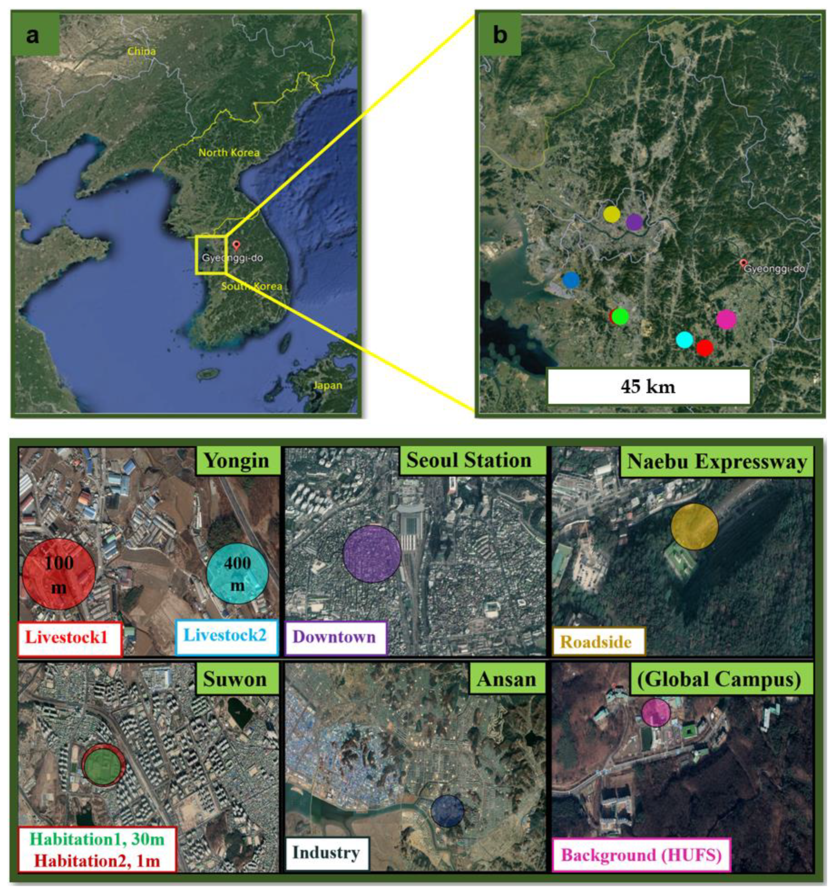
2.1. Site Description

The Seoul Metropolitan Area is the most populated region in South Korea accommodating approximately 50% of the country’s population, with a large presence of industrial, agricultural, and other human activities, due to which the ammonia emissions in these regions are comparatively higher than those in other regions across South Korea [36]. Changes in ammonia concentration depend on the weather, location, seasons, manner in which animals are bred, structural development, and operating method of management systems [4]. Due to the presence of both urban and rural areas in the Seoul metropolitan area, different types of locations were selected for measurements of ammonia concentration. A Background site, Hankuk University of Foreign Studies Global Campus (HUFS), was selected to establish the background ammonia concentration, and seven studied sites were chosen to measure the variation in ammonia concentration (Figure 1). Five sites were in the Gyeonggi province surrounding the capital city of Seoul, which is the most populated province in South Korea. Livestock 1 and 2 were two rural-agriculture sites in a northeastern region in Yongin (situated upwind from the source), 7 km from the Background (HUFS) site and 100 and 400 m from the ammonia source, respectively. Two suburban sites (Habitation 1 and 2) were chosen in Suwon, approximately 22 km from the HUFS; the sites were in the same building but at an elevation of 30 and 1 m, respectively. An industrial site (Industry) in Ansan was situated approximately 40 km from the HUFS. The majority of the industries in the Industry site are the manufacturers of electronics products, displays, chemicals, and medicines. Two studied sites in Seoul City were also studied. Seoul Station (Downtown) is in the heart of the city and has a very high density of traffic and population throughout the year.

The other Seoul City site was situated on one of the longest roads (Naebu expressway) in a tunnel through the Bukhan Mountain, a mountain located on the northern periphery of Seoul.

Table 1. Summary of studied sites with their location.

Site Name	Type	Latitude	Longitude	Sampler Type
Livestock 1 (at 100 m distance)	Rural-agricultural	37.31°	127.22°	Passive
Livestock 2 (at 400 m distance)	Rural-agricultural	37.31°	127.22°	Passive
Roadside	Suburban	37.61°	126.97°	Passive
Seoul Station	Urban	37.55°	126.98°	Passive
Industry	Industrial	37.27°	126.86°	Passive
Habitation 1 (at 30 m height)	Suburban	37.30°	126.96°	Passive
Habitation 2 (at 1 m height)	Suburban	37.30°	126.96°	Passive
Background (HUFS)	Rural	37.34°	127.26°	Passive/URG

Ammonia sampling was conducted for one year (March 2020–March 2021) at all studied sites.

presents a summary of the studied sites, describing the type of site and their longitude and latitude.

It has been shown from the type of sampler used, that ambient ammonia plays a key role in ammonia pollution by acting as a precursor in aerosol formation with atmospheric NO_x and SO₂ [37,38,39]. Therefore, it is essential to identify areas that have a higher concentration of ammonia emissions. Livestock regions were chosen because fertilizers and animal waste products generally emit ammonia [10,40,41,42]. Thus, measurements at these sites were used to validate the findings of previous studies.

2.2. Sample Collection and Lab Preparation

Seasonal and spatial variations in ammonia concentration were measured using a Radiello passive ammonia sampler (developed by Sigma-Aldrich, St. Louis, MO, USA) and an annular denuder (developed by University Research Glassware, Corp. Chapel Hill, NC, USA) (Supplementary Figure S1). The sampler consisted of a microporous polyethylene cylindrical cartridge (60 mm long and 4.8 mm wide) that was infused with phosphoric acid (H₃PO₄) to adsorb ammonia (part number (p/n): Sigma-Aldrich RAD168). The sampler consisted of a microporous cylindrical blue diffusive body, having a length of 60 mm, a diameter of 16 mm, a thickness of 1.7 mm, and an average porosity value of 25 μm, which was used to control the rate of diffusion (p/n: Sigma-Aldrich RAD1201). A polycarbonate plate (p/n: Sigma-Aldrich RAD 121) supported the blue diffusive body, and a vertical adapter (p/n: Sigma-Aldrich RAD 122) was used to fit the diffusive body with the supporting plate in a vertical or horizontal position. During preparation, all samplers were mounted outdoors at approximately 2 m above ground level in an inverted position with a rain shelter (p/n: Sigma-Aldrich RAD 196), as shown in Figure S2. All samplers were developed in the laboratory at the HUFS with new adsorption cartridges that were sealed in the factory during manufacturing. This was done on an ammonia-free laminar flow clean bench (model number (m/n): VS-1400 LVN), which was manufactured and sold by Vision. The sampler was placed inside the outer blue diffusive body, and an aluminum foil was used to wrap the outer body. The assembled sample was then placed into a 50 mL centrifuge tube, which was later sealed in a plastic bag with phosphoric acid-soaked paper towels on both surface and bottom to eliminate any traces of ammonia in the lock and lock box. The lock and lock box was stored in a moving box along with temperature and RH sensors, which were transported to the sampling site. The Radiello samplers were attached to the shelter every Monday for weekly ammonia sample collection between 30 March 2020 and 29 March 2021. We used a _1/2AA battery-operated temperature sensor (Lascar Electronics EasyLog USB, m/n: EL-USB-2-LCD+) for the passive sampler (Figure S3), to measure the temperature and relative humidity as the ammonia concentration was hypothesized to be affected by these factors. These sensors were mounted at the same height as each of the ammonia passive samplers. Ammonia concentrations were obtained by collecting samples across all eight studied sites continuously over one year, spanning four different seasons in Korea. After the sampling period, the samples were sealed in a 50 mL centrifuge tube in a plastic bag with a phosphoric acid-soaked paper towel in a lock and lock box, and placed in an ammonia-free clean freezer at a temperature between −15 and 0 °C. These were sent back to the laboratory at 4-week intervals from the sampling site. Using the same transportation methods [43], samples were returned to the laboratory where they were placed in a clean ammonia-free freezer until the cartridge was extracted. The blue diffusive bodies were cleaned with 18.2 MΩ cm deionized water (DI) and sonicated twice at 20 min intervals for more than 40 min after every use. This was done to reduce contamination of the passive sampler.

The denuders were developed in the HUFS lab a day before installation on the site. They were stored separately in a sealed plastic bag in a refrigerator at 2–6 °C overnight before installation.

2.3. Passive Sampler

Passive ammonia samplers have been used in various studies to measure concentration because of their external energy-free design, quick installation, and reliability [43,44,45,46,47]. The samplers consisted of a cylindrical outer surface that acted as a diffusive membrane, allowing gaseous molecules to travel in a direction parallel to the adsorbent bed that was cylindrical and coaxial to the diffusive surface. The cartridge was injected with phosphoric acid (H₃PO₄) [48].

The ammonia concentration was determined by considering the passive sampler characteristics and the rate of ammonia diffusion in the air. The diffusion index (${\mathrm{Diff}}_{{\mathrm{NH}}_3}$), which is a function of local temperature ($\mathrm{Temp}$) and ambient pressure ($\mathrm{Pres}$), can be represented using Equation (1) as:

$${\mathrm{D}}_{\mathrm{iff}}\left(\mathrm{Temp}, \mathrm{Pres}\right)={\mathrm{D}}_{\mathrm{iff}0,1}\times \left(\frac{{\mathrm{Pres}}_0}{\mathrm{Pres}}\right)\times {\left(\frac{\mathrm{Temp}}{{\mathrm{Temp}}_0}\right)}^{1.81}$$

(1)

where ${\mathrm{Diff}}_{0,1}$ = 0.1978 cm²/s, with subscript 0 being the ${\mathrm{Temp}}_0$ value (273 K (0 °C)) and subscript 1 being the Pres₀ value (1 atm) [49]. The local pressure was determined using the height of the site above sea level, while the temperature was obtained using a temperature sensor. The rate of flow of diffusion (${\mathrm{QF}}_{\mathrm{rate}})$ within the ammonia passive sampler was determined using Equation (2) [50]:

$${\mathrm{QF}}_{\mathrm{rate}}={\mathrm{Diff}}_{{\mathrm{NH}}_3}\left(\mathrm{Temp}, \mathrm{Pres}\right)\times \frac{\mathrm{A}}{\mathsf{\Delta }\mathrm{x}}$$

(2)

where A is the cross-sectional area of the passive sampler, and $\mathsf{\Delta }\mathrm{x}$ is the distance of diffusion in the passive sampler in this experiment. A/$\mathsf{\Delta }\mathrm{x}$ represents the constant value for the flow in the radial section of the ammonia passive sampler and has been noted to have a value of 14.2 cm, which is based on experimental measurements. The ammonia concentration present in the surrounding air (${\mathrm{C}}_{{\mathrm{NH}}_3}$) was determined using Equation (3) from the rate of flow of diffusion (${\mathrm{QF}}_{\mathrm{rate}}$) in mL/min, the time taken for sampling (t) in minutes, and the total amount of ammonia deposited on the cartridge (${\mathrm{m}}_{{\mathrm{NH}}_3}$) in $\mathsf{\mu }\mathrm{g}$ [50]:

$${\mathrm{C}}_{{\mathrm{NH}}_3}\left({\mu \mathrm{g} \mathrm{m}}^{-3}\right)=\frac{{\mathrm{m}}_{{\mathrm{NH}}_3\left(\mu \mathrm{g}\right)} }{\mathrm{t}\times {\mathrm{QF}}_{\mathrm{rate}}}$$

(3)

Final concentrations were recorded in µg m⁻³ and converted into ppb by using Equation (4):

$${\mathrm{C}}_{{\mathrm{NH}}_3}\left(\mathrm{ppb}\right)=22.41\times \left(\frac{\mathrm{Temp}}{{\mathrm{Temp}}_0}\right)\times \frac{{\mathrm{Pres}}_0}{17.031}\times {\mathrm{C}}_{{\mathrm{NH}}_3}\left(\mu \mathrm{g} {\mathrm{m}}^{-3}\right)$$

(4)

where 22.41 is the volume of an ideal gas (L mol⁻¹) at standard temperature and pressure (STP), Temp is the ambient temperature in °C, Temp₀ = 273.15 K (0 °C), Pres₀ is the atmospheric standard pressure (1 atm), 17.031 is the molecular weight of ammonia, and ${\mathrm{C}}_{{\mathrm{NH}}_3}$ is the ammonia concentration in μg m⁻³.

2.4. Annular Denuder

An annular denuder was installed at the Background (HUFS) site to measure the concentration of gaseous ammonia on a weekly basis for a correctness study [51]. The denuder was coated with a denuder coating solution of a mixture of 10 g phosphoric acid (H₃PO₃ 80%), 100 mL deionized water (DI) (ULTiMA DUO, RO, and UP System), and 900 mL methanol (CH₃OH 99.75%). The denuder was filled with 15 mL of the prepared solution and, once the solution dissolved into the denuder, it was left to stand for 30 min until a coating formed on it. Using a Rotameter, the denuder was attached to a URG glass-drying manifold and connected to a nitrogen gas tank with a 6 PSI flow rate, for a minimum of 90 min. The denuder was turned upside down every 15 min during drying [48]. Once the denuder was dried, a polyvinylidene fluoride (PVDF) inlet tubing line was connected to it. PVDF was used because of its low ammonia adsorption quality [52]. Atmospheric ammonia was collected using a PVDF inlet tubing with a diameter of 6.35 mm and a Teflon filter pack (PTFE membrane, pore size 0.45 µm, Advantech Pall Corporation) with a diameter of 47 mm, through which the air passed. During the air passage, fine particles were also collected on the H₃PO₃-coated denuder to collect any extra ammonia from the ammonium salt particles deposited on the Teflon filter [53]. Both the denuder and passive samples were simultaneously changed at the Background (HUFS) site. Airflow was provided using a Thomas Piston Pump 2660 Series vacuum pump, which was controlled using a straight 0.4 mm orifice fitting, designed to fix the airflow rate by restricting it with a significantly smaller orifice on the threaded side of the fitting. It had a 4 mm push-in fitting on one side and a 9.728 mm male threaded port on the other side. The push-in fitting provided an easy connection with the tubing. The tube was pushed in, and the fitting was fixed using stainless steel clamps. The pump was also suitable for vacuum applications at a pressure of −1 bar (−14.5 psi) and had nitrile butadiene rubber (NBR) seals (Pisco 0.4 mm Orifice, Tameson) that made it suitable for applications within a temperature range of 0–60 °C. A portable gas flow meter (SIARGO, m/n: MF5706), which had a wide application range with fewer constraints on power, temperature, and pressure consumption, was installed between the denuder and orifice to provide a continuous rate of air flow. The sample flow read by the portable gas flow meter was corrected to ambient conditions by matching the pressure drop through the denuder and filter. The annular denuder and related sampling components were set up in the lab with the annular denuder mounted on a clamp stand are shown in (Figure S4). The constant total flow rate through the systems was approximately 1.35 L per min (LPM), which was calculated using Equation (5):

$${\mathrm{QF}}_{\mathrm{v}}\left(\mathrm{LPM}\right)={\mathrm{QF}}_{\mathrm{s}}\left(\mathrm{SLPM}\right)\times \left(\frac{{\mathrm{P}}_{\mathrm{s}}}{{\mathrm{P}}_{\mathrm{i}}}\right)\times \left(\frac{{\mathrm{T}}_{\mathrm{i}}}{{\mathrm{T}}_{\mathrm{s}}}\right)$$

(5)

where QF_v (LPM) is the desired ambient volumetric flow rate, QF_s (SLPM) is the flow rate under standard conditions, P_i is the ambient pressure, P_s is the standard condition pressure, T_s is the standard condition temperature, and T_i is the ambient temperature. The annular denuder established a standard of comparison for assessing the effectiveness of the ammonia passive samplers. This method has been used in previous studies because of its verified efficiency in gas and particle sampling [48,54,55]. Finally, the ammonia denuder concentration (µg m⁻³) was calculated using Equation (6):

$${\mathrm{C}}_{{\mathrm{NH}}_3}\left({\mu \mathrm{g} \mathrm{m}}^{-3}\right)=\frac{\left(0.994\times {\mathrm{C}}_{{\mathrm{NH}}_4^{+}}\left(\mathsf{\mu }\mathrm{N}\right)\times {\mathrm{V}}_{\mathrm{ext}}\left(\mathrm{L}\right)\times {\mathrm{MW}}_{{\mathrm{NH}}_4^{+}}\right)}{{\mathrm{V}}_{\mathrm{act}.\mathrm{air}}\left({\mathrm{m}}^3\right)}$$

(6)

where ${\mathrm{C}}_{{\mathrm{NH}}_3}$ is the calculated ammonia concentration (μg m⁻³), where g represents gram-equivalent and ${\mathrm{C}}_{{\mathrm{NH}}_4^{+}}$ $\left(\mathsf{\mu }\mathrm{N}\right)$ is the ammonium concentration measured during the extraction from the denuder. The volume for extraction (V_ext) was 0.01 L, and ${\mathrm{MW}}_{{\mathrm{NH}}_4^{+}}$ is the molecular weight of NH₄⁺. The ratio of molecular weights of NH₃ and NH₄⁺ (0.994) was used to convert the measured amounts of NH₃ and NH₄⁺ [54,56].

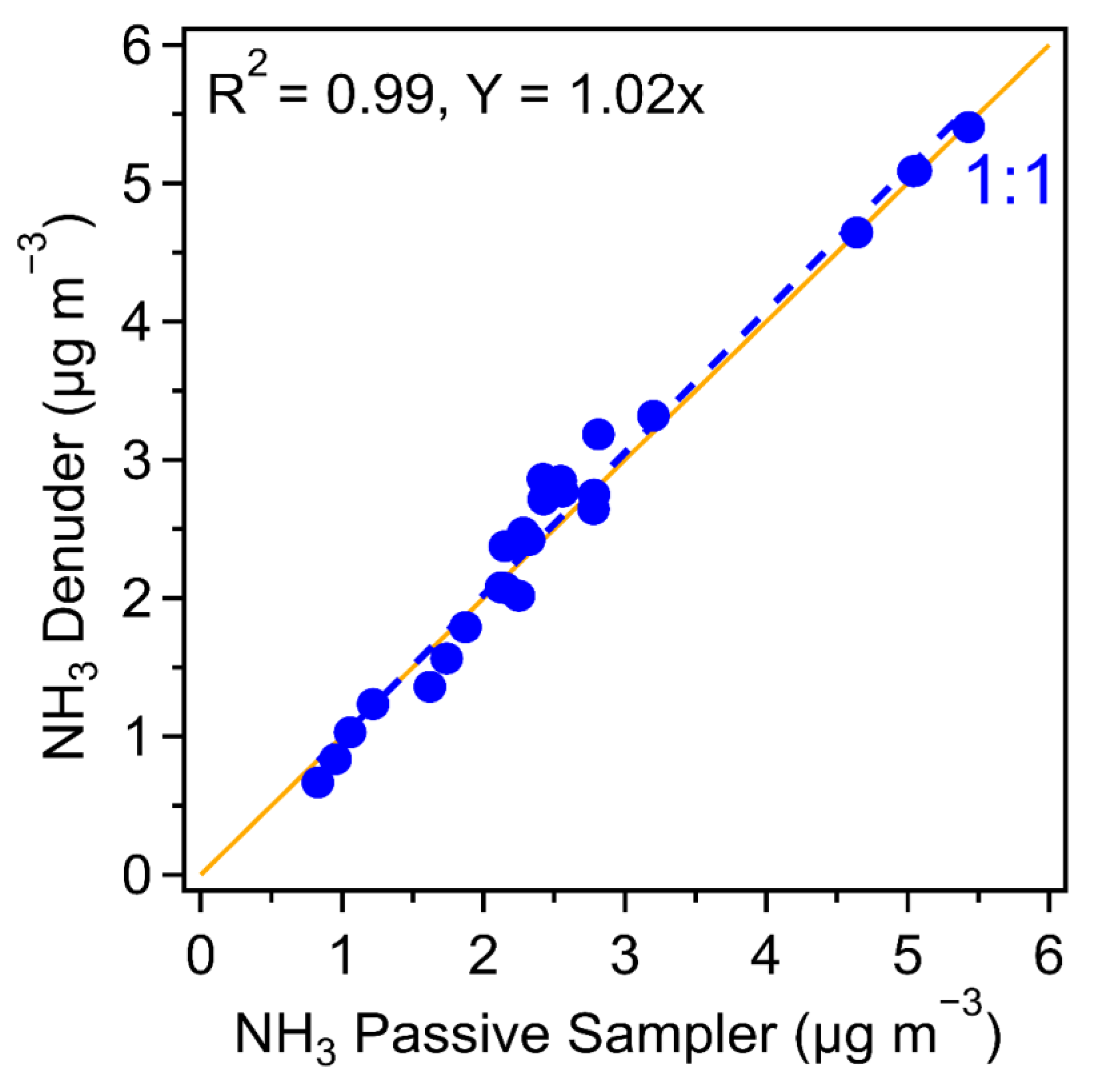
2.5. Qualitative and Quantitative Analysis

Annular denuders and ammonia passive samplers were obtained from the laboratory at the HUFS. Samples were extracted from the annular denuder by adding 18.2 MΩ cm deionized water (DI) and then hand-rotating them continuously for 60 min before they were stored in a 10 mL falcon tube. The samples were analyzed using ion chromatography, and the ammonia passive sampler cartridges were extracted with a power sonic (Hwashintech, 510 sonicate instrument) for a total duration of 55 min in 10 mL DI. Ion chromatography was used to analyze the passive sampler. The cations present in the samples were segregated using 20 mM methane sulfonic acid (CH₃SO₃H) solvent (1 mL min⁻¹) on a Dionex Aquion, CS12A column, Dionex ion Pac CG12A guard column, ion-exchange chromatography column configured with a 100 $\mu$L sample loop, and a 4 mm Dionex CERS 500 suppressor using a Dionex conductivity detector and a 2014 ICS-1100 Autosampler.

Ion chromatography, passive quality control, and quality assurance tests were performed on the sampler to accurately measure the concentration. Accuracy was measured by calculating the difference obtained between the concentration of the standard solution (Kanto Chemical Co. Ltd., Tokyo, Japan) of the analyte and the concentration of the analyte solution calculated using ion chromatography. Accuracy is a measure of error, which can be defined in two ways. The absolute error is the difference between the measured and standard values of the solution concentration. The relative error, expressed in the form of a ratio, is the second measure of error. Formulae for measuring both accuracy values are shown in Supplementary Equations (S1) and (S2), respectively. Precision is defined as the deviation from the standard solution measurement and was obtained by continuously repeating the measurement; it was higher if the ratio of the deviation value to the measured value (as measured by ion chromatography) was lower. Precision can be measured using two methods: analytical precision, which is the ratio of the deviation value to the measured value of the standard solution, and measurement precision, which is the deviation of the measured value from the experimental value of the entire sample. The formulae used to measure the precision values are given in Equations (S3) and (S4), respectively. To measure both accuracy and precision, an additional ammonium 200 ppb standard solution was analyzed at frequent intervals during sample analysis. Ammonia concentration was measured as follows: Replicated Radiello ammonia passive samplers were collected from all eight studied sites to measure the performance of the ammonia passive samplers under varying conditions and sampling periods. The experimental value for accuracy (the absolute error value) was 0.20 ppb, and the relative error value was 0.10%. The analytical precision was 0.95%, with a pooled relative standard deviation (RSD) of 3.8% (N = 212), indicating a strong correlation between the 1st and 2nd replicate samples (R² = 0.999 and slope = 0.998), as shown in (Figure S5). The weekly ammonia concentrations collected by the passive samplers at the Background (HUFS) site, indicated a strong correlation coefficient (R² = 0.99, slope = 1.02) for the sample data (N = 25) obtained from the annular denuder located at the same site (Figure 2). A high R² value signified a reliable design for measuring ammonia concentration and high accuracy at the studied sites. Blanks from the field and laboratory were sampled for 1 year and were used to determine the minimum detection limit (MDL) by using (Equation (S5)). The concentration of ammonia in the blanks ranged from 0.015 to 0.19 ppb, with a mean value of 0.08 ppb and a standard deviation of 0.04 ppb. Field blanks were used to calculate the MDL, which was found to be 0.07 ppb for a Radiello passive ammonia sample collected over a week. (Figure S6) shows a graph of the measured values used to calculate the accuracy and MDL. The detailed QC/QA analysis values and calculations are presented in Supplementary Table S1.

3. Results and Discussion

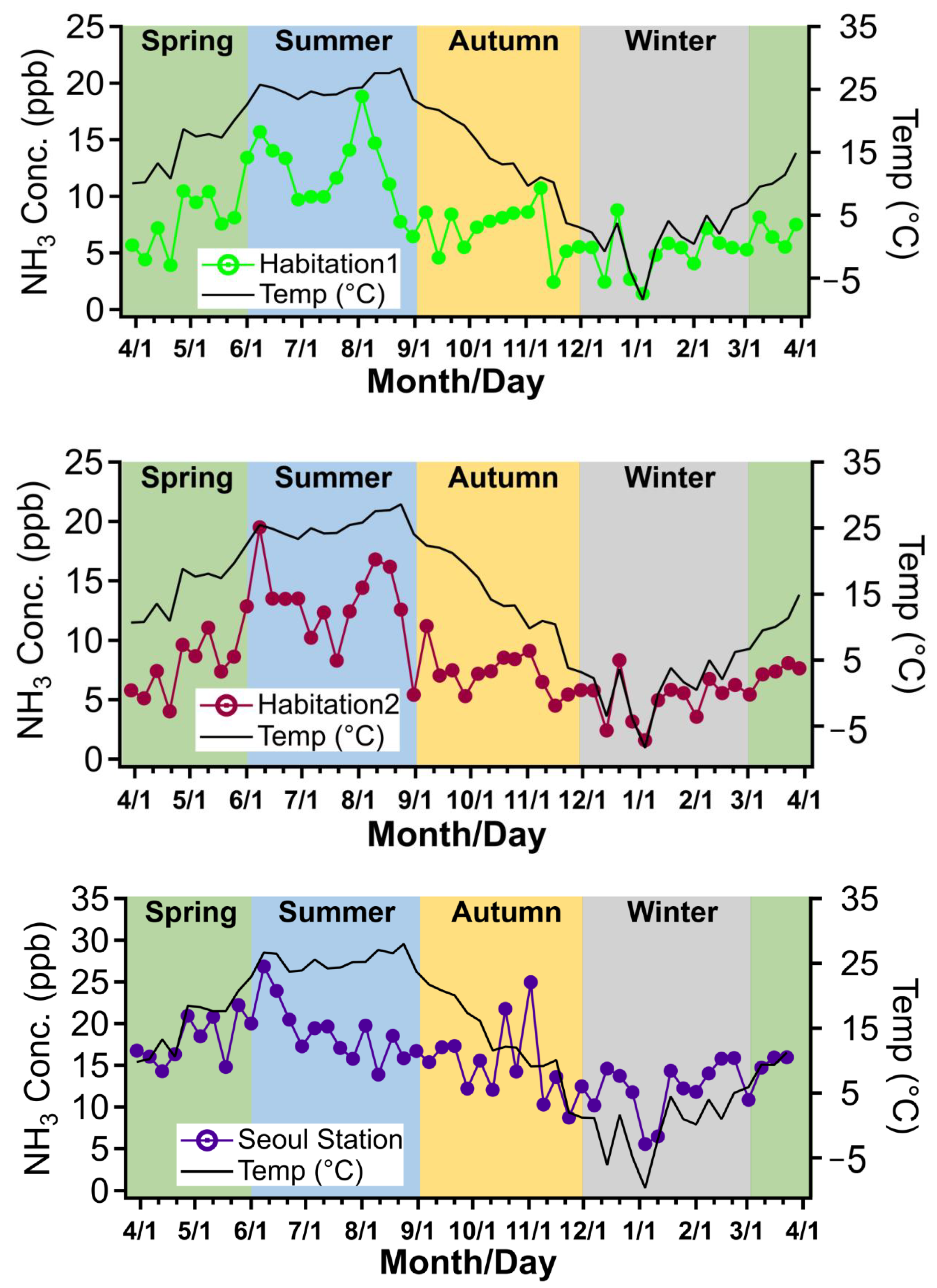
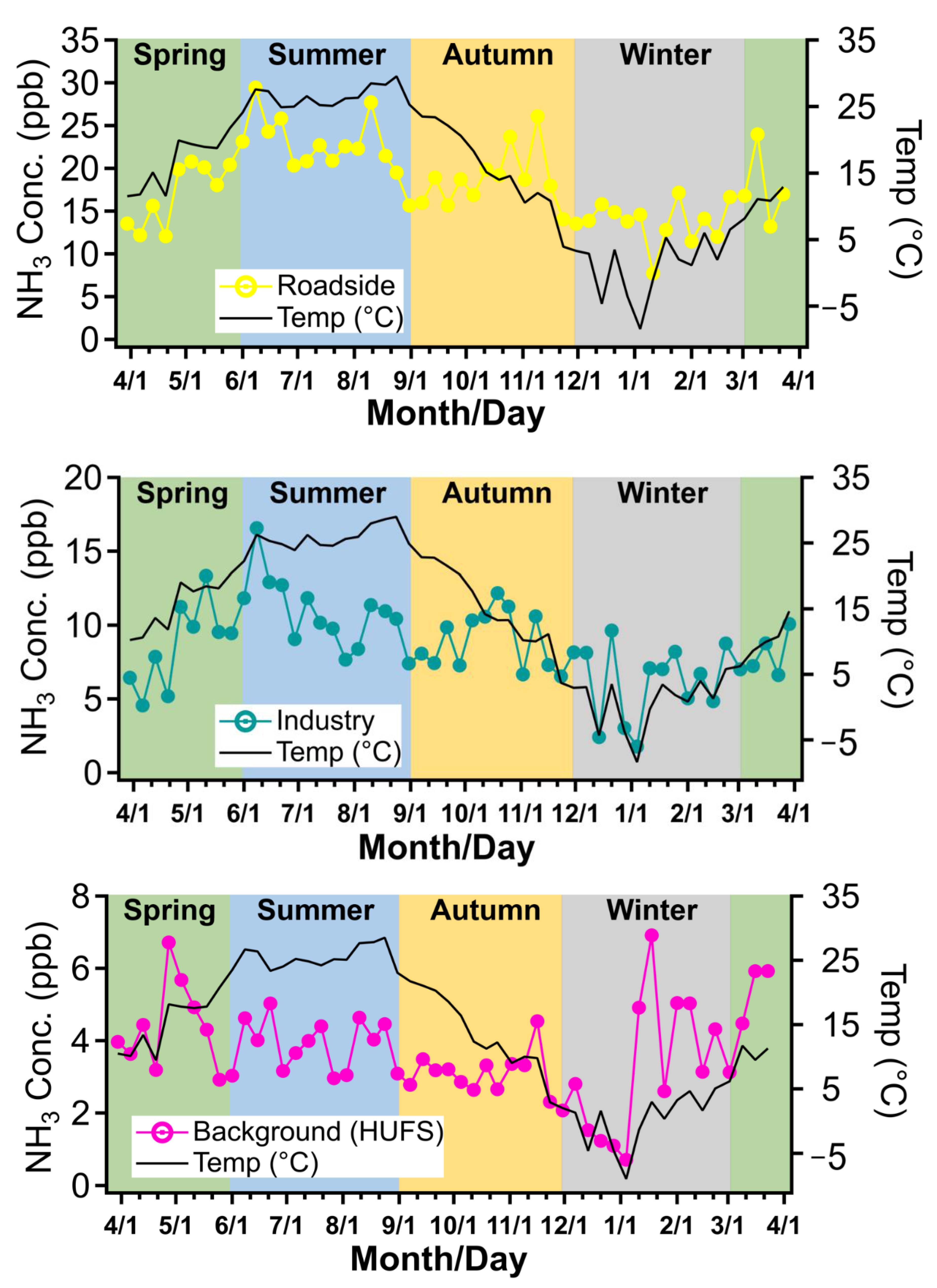
3.1. Seasonal Variation in Ammonia Concentration

Atmospheric ammonia concentrations are largely associated with ammonia emissions from local regions [57]. The results from this study identified a relationship between seasonal variations in ammonia concentration and multiple atmospheric conditions. The average seasonal ammonia concentrations at the studied sites are shown in Table S2 and Figure 3; the variation in concentration with temperature and relative humidity is shown in Supplementary Figure S7.

Figure 3 shows that during all four seasons, the Livestock 1 and 2 sites had notably higher concentrations than any other studied sites, with maximum concentrations during the autumn. Studies have indicated that emissions from animals during summer are almost twice as high as those in winter due to temperature increases and manure processing during summer and autumn. The high autumn ammonia concentrations were mostly likely due to low rainfall, which did not dilute or leach nitrogen from the soil slurry in the farming regions [58]. In addition, the increased use of fertilizers [59] and manure processing in the farm fields [6,17] during this time also likely resulted in a high ammonia concentration. Studies have also shown that the daily emission rate of ammonia is highest in the autumn–winter period, due to more pig fattening at this time, and that agricultural floors with daily manure removal have significantly lower emissions than concrete agricultural floors [60]. Ammonia concentration is also affected by the age and weight of the animals, the amount of urea in their urine, and amount of undigested nitrogen in the pig feces [61]. The pH of manure is another factor that affects the release of ammonia, with lower concentrations when the pH drops below 7 [62]. Therefore, the livestock regions contributed heavily to ammonia emissions in northeastern South Korea during the autumn.

Ammonia emissions, which plays a crucial role in particulate matter formation, were less dependent on the season in urban locations, which may be crucial for affecting the particulate matter concentrations. The two sites in Seoul city (Seoul Station and Roadside), had similar ammonia concentrations which peaked during the summer [63]. High concentrations of ammonia in summer can be attributed to the greater usage of personal vehicles [64]. Ammonia concentration at the Industry site was also peaked during summer; however, overall, the seasonal ammonia concentration was lower than at the Livestock and Seoul city sites. Ammonia concentration varied at the Habitation 1 and 2 sites, peaking during summer but also increasing with an increase in temperature, humidity, and air velocity [61,65]. However, there was no relationship between the increase in ammonia concentration during winter and domestic heating; thus, household gas combustion was not considered to be an emission source.

The Background (HUFS) site recorded the lowest ammonia concentrations due to its rural location, with negligible industrial or agricultural activities in the surrounding area.

With the exception of the Background (HUFS) site, all of the studied sites recorded the lowest ammonia concentrations during winter, which agrees with the findings of previous ammonia measurement studies [66]. This decrease in ammonia concentration during the winter has been linked to the formation of NH₄NO₃ (ammonium nitrate) particulates [6,67,68,69].

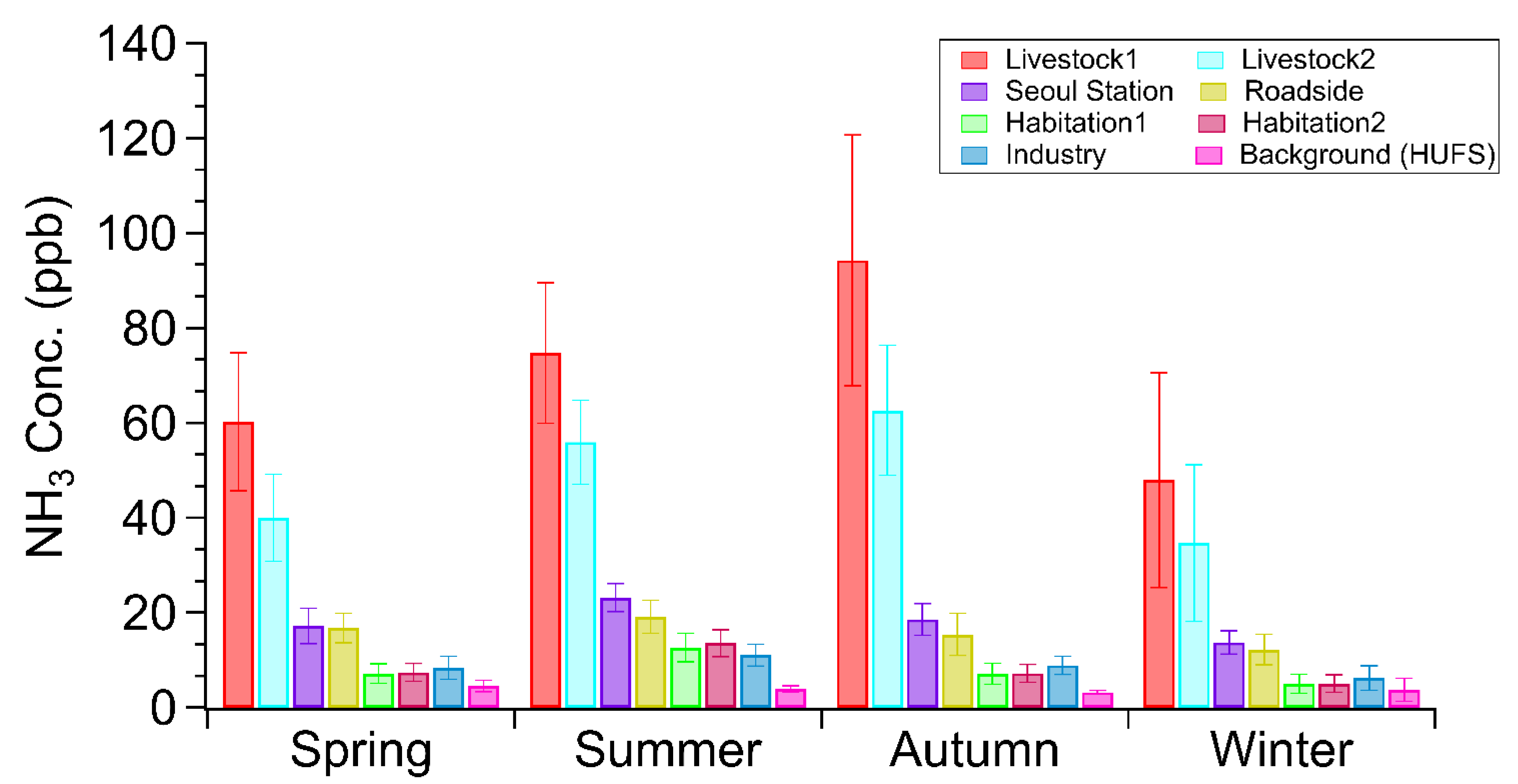
3.2. Spatial Distribution of Ammonia Concentration

Table 2. Annual average concentration and standard deviation of ammonia (ppb) at studied sites.

Sites	Average	Standard Deviation
Livestock 1	69.3	26.3
Livestock 2	48.3	16.7
Seoul Station	18.2	4.6
Roadside	15.9	4.3
Habitation 1	8.0	3.6
Habitation 2	8.3	3.8
Industry	8.6	2.8
Background (HUFS)	3.8	1.5

shows the annual average ammonia concentration, and Figure 4 shows the annual variation in ammonia concentration and temperature at all of the studied sites; the annual ammonia concentrations in the regions surrounding Seoul are shown in Figure S8. High ammonia concentrations in livestock regions show that the agricultural use of fertilizers and emissions from animals were the primary sources of ammonia in these regions. Surprisingly, ammonia emissions in the densely populated areas of Seoul were lower than in the livestock regions, suggesting that vehicles do not produce as much ammonia as livestock. Industries in the Ansan region also had low ammonia concentrations, signifying that these industries do not contribute much to atmospheric ammonia emissions. Ammonia concentrations in Seoul City municipal sites were much greater than those in suburban Habitation 1 and 2 sites. This is supported by research that identified high ammonia concentrations in municipalities with high population and traffic density in the heart of crowded areas and high-rise buildings. Ammonia emissions from road traffic, uncovered decomposing trash dumps, and domestic burning could also contribute to this trend [70]. The Background site is in a mountainous region surrounded by relatively dense forests and had the lowest ammonia concentration among all the studied sites.

When ammonia enters the atmosphere it reacts with air pollutants, primarily nitrogen and sulfuric oxide molecules from nearby automobiles, power plants, and factories, to generate PM_2.5, which can travel great distances. Hence, ammonia emissions from one region of the country can affect air quality in other regions [71]. As vegetation emits very small amounts of ammonia, increased emissions seen during the spring are more likely to be linked to agricultural operations such as premature fertilizer application or seasonal variations in cattle feed availability and the accompanying emissions [72,73]. Furthermore, several studies have confirmed that in livestock areas, the ammonia concentration in summer is nearly double the concentration in winter [74,75,76,77].

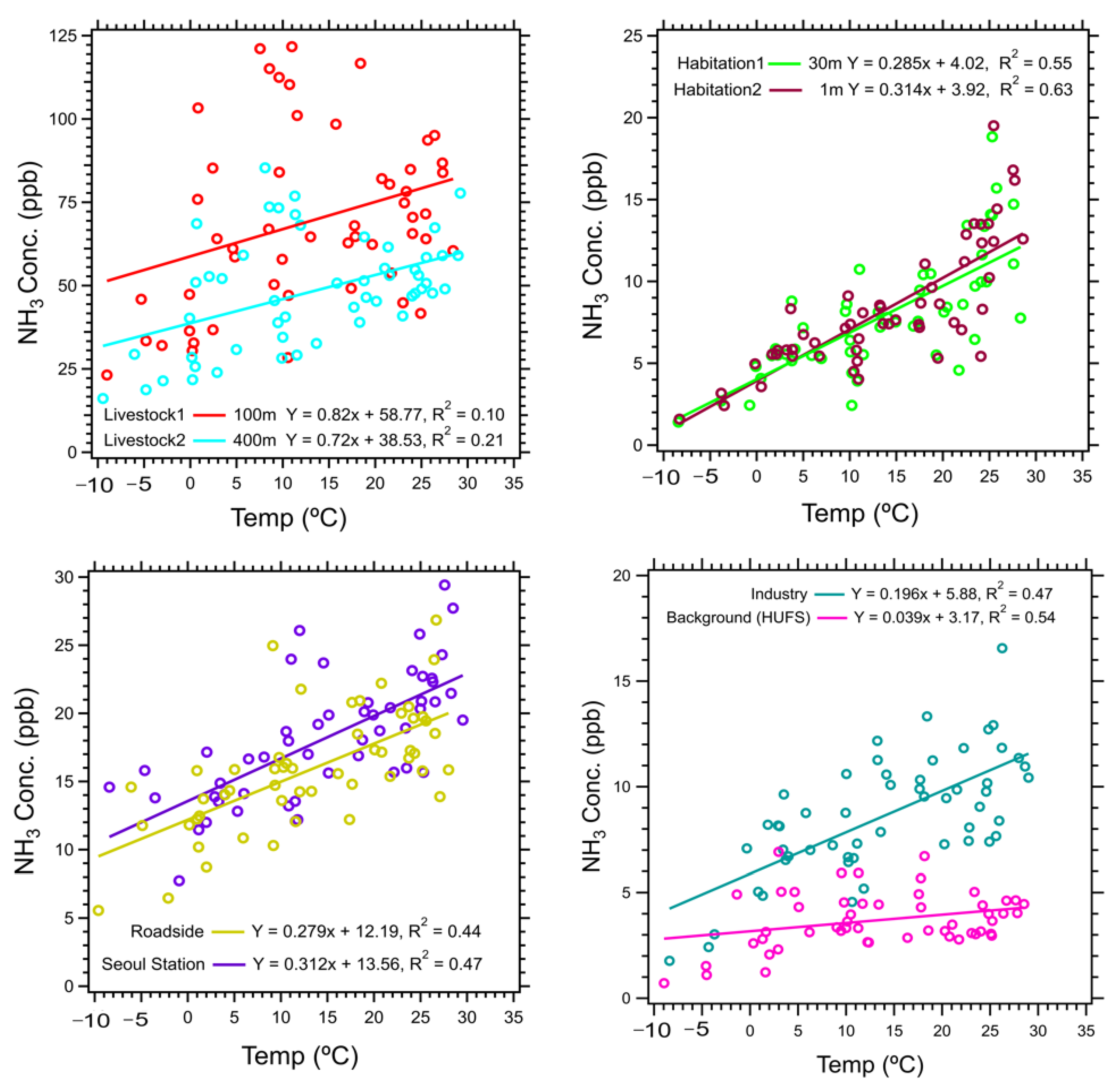
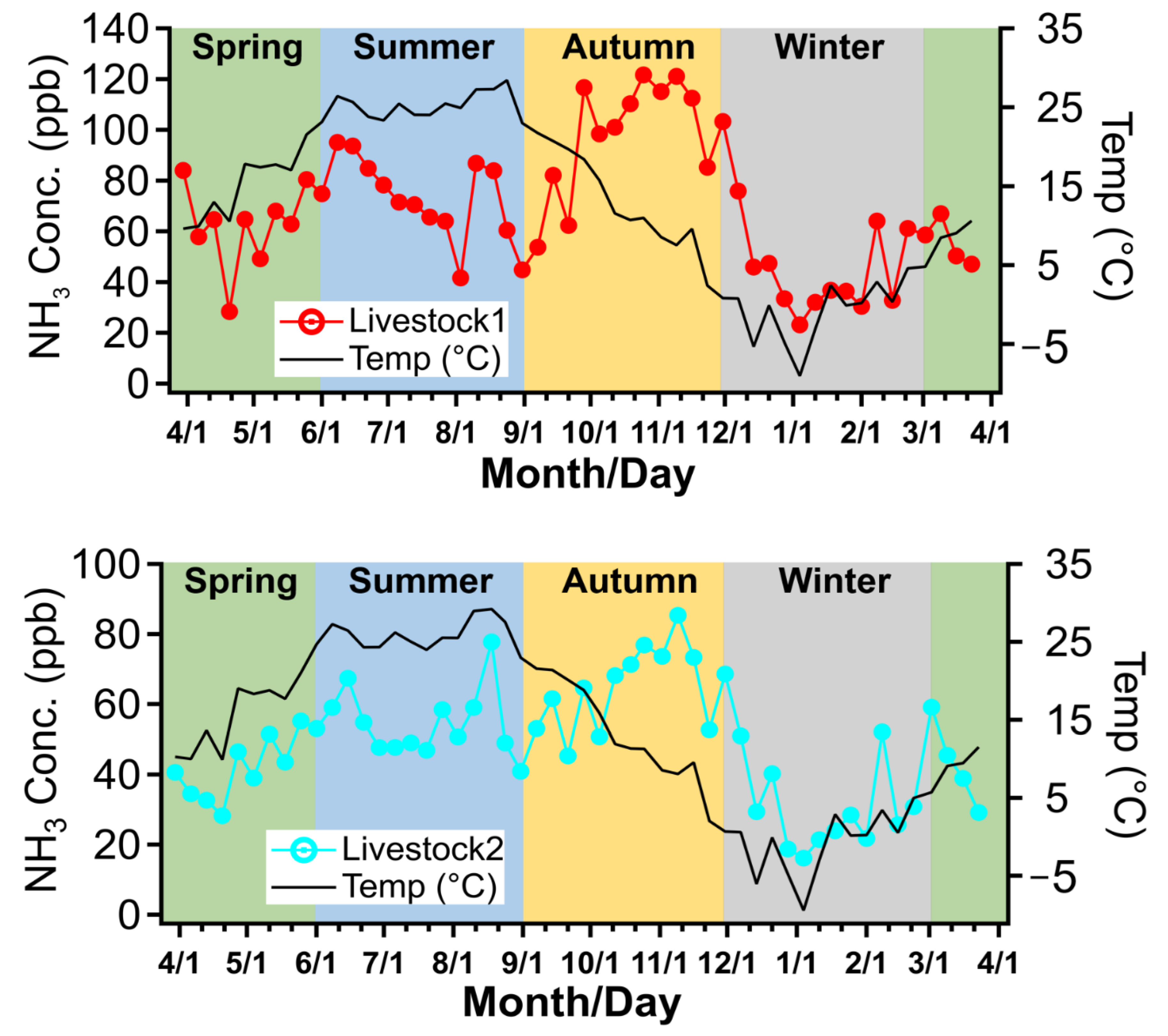
3.3. Correlation between Ammonia Concentration and Temperature

Figure 5 shows the variation in ammonia concentration with temperature and the coefficient correlation (R²) values of all studied sites. The R² values at the Livestock 1 and 2 sites were 0.10 and 0.21, respectively. The R² values at the Seoul station and Roadside sites were 0.47 and 0.44, respectively. The industrial region in Ansan had an R² value of 0.47, and the Habitation 1 and 2 sites had R² values of 0.55 and 0.63, respectively. Finally, the Background site had an R² value of 0.54. Many of the sites had R² values of approximately 0.5 or higher, indicating that temperature played a significant role in ammonia concentration, particularly at the Seoul station, Roadside, and Habitation 1 and 2 sites.

There have been many studies that have shown a correlation between ammonia concentration and temperature. Pederson et al. (2021) found that if the ground was moist, there was a positive correlation between ambient temperature and ammonia emissions [77]. Wang et al. (2020) also found a positive correlation between ammonia concentration and ambient temperatures in urban areas, leading to particularly high ammonia concentrations during summer [78]. A similar effect was observed by Li et al. (2017), but only at high altitudes [48]. Laboratory experiments to establish a correlation between temperature and ammonia emissions from cow manure and fertilizers also found that ammonia emissions were greater at higher temperatures [79]. This agrees with our finding that in livestock regions ammonia emissions are higher in summer, compared to that at the other studied sites. It has also been found that higher concentrations of atmospheric ammonia are emitted in agricultural areas due to the chemical instability of the ammonium nitrate compound which is used to produce fertilizers [80].

These previous studies show that ammonia concentration is dependent on ambient temperature, and our study further establishes that an increase in the ambient temperature leads to an increase in the ammonia concentration. Therefore, an increase in temperature is a key factor influencing ammonia pollution. Vehicular pollution, agricultural fertilizers, and animal husbandry are common primary sources of ammonia, and these activities must be monitored, especially during periods of high temperatures.

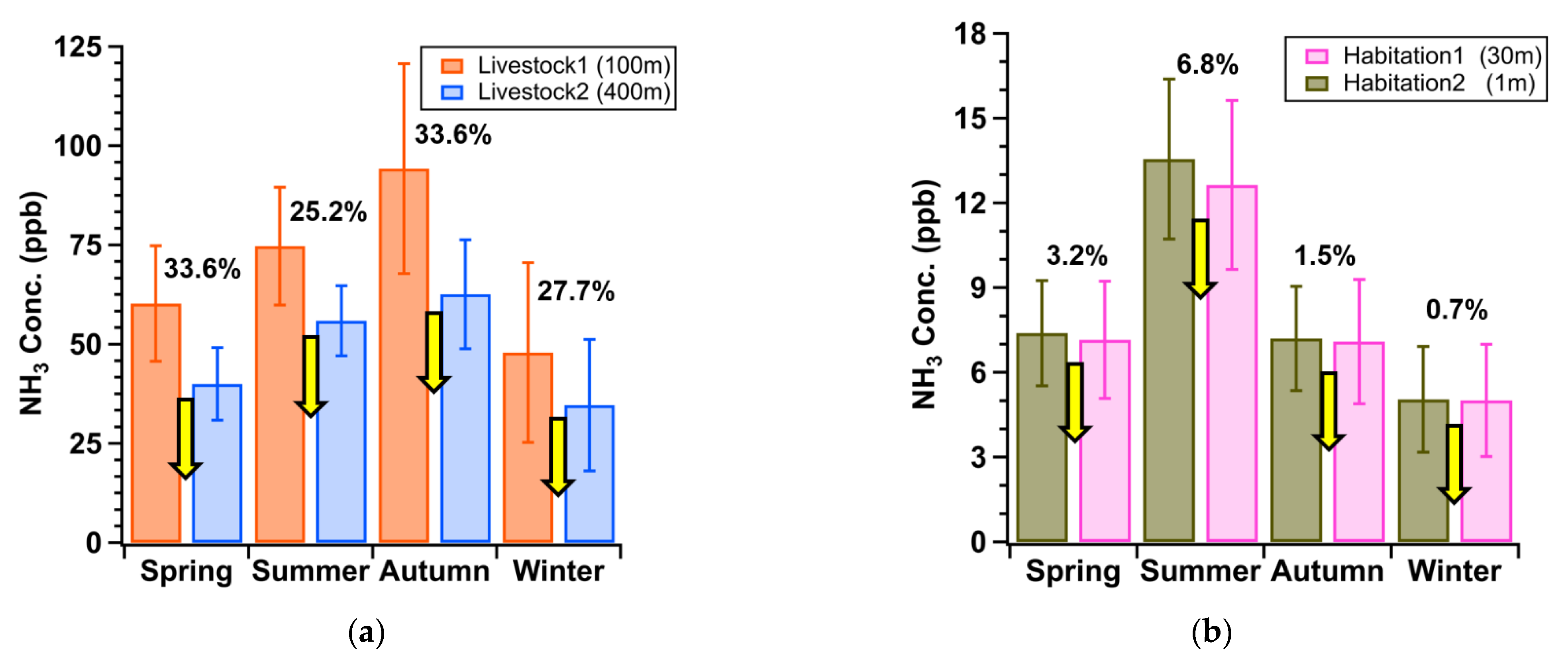
3.4. Habitation and Livestock Region Analysis

While only one sampler was installed at most of the studied sites, the Livestock and Habitation sites had two samplers each because two separate measurements were done at both of these sites. This was done to analyze the variation in ammonia concentration with distance from the pig farm and height above the ground. Livestock site data were collected at 100 and 400 m from the pig farm, and Habitation site data were collected at heights of 1 and 30 m above ground level. Figure 6 shows the ratio of change in concentration to the change in height for the Habitation site and the ratio of change in concentration to change in distance for the Livestock site.

It has been reported that ammonia concentration increases with an increase in temperature above a specific height and is usually unaffected at ground level [48]. This generally agrees with our findings, wherein Habitation sites 1 and 2 had similar ammonia concentrations. However, Habitation 2 (1 m) did have a slightly higher ammonia concentration than Habitation 1 (30 m). This difference is likely due to the higher temperature and human activity at ground level. Furthermore, the change in ammonia concentration with altitude varied by 1–3% depending on the season.

Livestock 1 (100 m) and 2 (400 m) had significantly different ammonia concentrations, despite being located relatively close to each other, with Livestock 1 exhibiting a significantly higher ammonia concentration as it was closer to the pig farms. Furthermore, the change in the ammonia concentration with distance from the pig farm varied by 28–34% depending on the season, as the distance from the emission source increased by approximately 300 m.

4. Conclusions

This study verified seasonal and regional variations in ammonia concentrations and demonstrated that regions with high agricultural activities result in increased ammonia emissions. This highlights the need to reduce the usage of ammonia-based fertilizers, in order to reduce the harmful effects of ammonia pollution on the population in and around these regions. Ammonia concentrations in the densely inhabited parts of Seoul and in the industrial areas were significantly lower than the emissions from the livestock zones. Among all the studied sites, the HUFS had the lowest ammonia concentration due to its rural location, which was less densely populated and had negligible agricultural or industrial activity in the surroundings.

Studies have indicated that emissions from animals during summer are almost twice as high as those in winter due to temperature increases and manure processing during summer and autumn. In this study, most of the sites recorded peak ammonia concentrations during summer, indicating that high temperatures are responsible for high ammonia concentrations. This study observed a unique trend, with the highest ammonia concentrations in livestock regions with prevalent agricultural and animal husbandry activities being observed during autumn. Low rainfall led to increase in ammonia concentrations, since rainfall causes nitrogen leaching and removes the ammonia from the soil. The ammonia emission rate is also affected by pig fattening, which is high during fall and winter and low during summer and spring. Other key influencing factors on the ammonia concentration are the concrete agricultural floor, the animal’s age and weight, urea content in urine, and undigested nitrogen in feces. The ammonia concentration also increases when the pH of the manure is greater than 8.

This study highlights that agricultural activities are one of the leading causes of the increase in ammonia pollution in the Seoul metropolitan region. It has also been shown that increased ammonia levels and residential heating during winter were unrelated. Thus, there is a need to monitor activities such as vehicle emissions, agricultural fertilizers, and animal husbandry during high-temperature periods, to minimize the effect of ammonia emissions on humans and the environment [50].

References

1. Pio, C.A.; Nunes, T.V.; Leal, R.M. Kinetic and thermodynamic behavior of volatile ammonium compounds in industrial and marine atmospheres. Atmospheric Environment. Part A Gen. Top. 1992, 26, 505–512. [Google Scholar] [CrossRef]
2. Huang, R.-J.; Duan, J.; Li, Y.; Chen, Q.; Chen, Y.; Tang, M.; Yang, L.; Ni, H.; Lin, C.; Xu, W.; et al. Effects of NH3 and alkaline metals on the formation of particulate sulfate and nitrate in wintertime Beijing. Sci. Total Environ. 2020, 717, 137190. [Google Scholar] [CrossRef]
3. Budavari, S. The Merck Index: An Encyclopedia of Chemicals, Drugs, and Biologicals, 12th ed.; Merck: Rahway, NJ, USA, 1996. [Google Scholar]
4. Pinder, R.W.; Gilliland, A.B.; Dennis, R.L. Environmental impact of atmospheric NH3emissions under present and future conditions in the eastern United States. Geophys. Res. Lett. 2008, 35. [Google Scholar] [CrossRef]
5. Haber, F. The Haber Process. Nature 1923, 111, 101–102. [Google Scholar]
6. Paulot, F.; Jacob, D.J.; Pinder, R.W.; Bash, J.O.; Travis, K.; Henze, D.K. Ammonia emissions in the United States, European Union, and China derived by high-resolution inversion of ammonium wet deposition data: Interpretation with a new agricultural emissions inventory (MASAGE_NH3). J. Geophys. Res. Atmos. 2014, 119, 4343–4364. [Google Scholar] [CrossRef]
7. Nelson, A.R.L.E.; Ravichandran, K.; Antony, U. The impact of the Green Revolution on indigenous crops of India. J. Ethn. Foods 2019, 6, 8. [Google Scholar] [CrossRef] [Green Version]
8. Randive, K.; Raut, T.; Jawadand, S. An overview of the global fertilizer trends and India’s position in 2020. Miner. Econ. 2021, 34, 371–384. [Google Scholar] [CrossRef]
9. Bray, C.; Battye, W.; Aneja, V.; Tong, D.; Lee, P.; Tang, Y. Impact of Wildfires on Atmospheric Ammonia Concentrations in the US: Coupling Satellite and Ground Based Measurements. In Proceedings of the 1st International Electronic Conference on Atmospheric Sciences, Online, 16–31 July 2016; p. 1. [Google Scholar]
10. Groenestein, C.; Hutchings, N.; Haenel, H.; Amon, B.; Menzi, H.; Mikkelsen, M.; Misselbrook, T.; van Bruggen, C.; Kupper, T.; Webb, J. Comparison of ammonia emissions related to nitrogen use efficiency of livestock production in Europe. J. Clean. Prod. 2019, 211, 1162–1170. [Google Scholar] [CrossRef]
11. Maasikmets, M.; Teinemaa, E.; Kaasik, A.; Kimmel, V. Measurement and analysis of ammonia, hydrogen sulphide and odour emissions from the cattle farming in Estonia. Biosyst. Eng. 2015, 139, 48–59. [Google Scholar] [CrossRef]
12. Shi, Z.; Sun, X.; Lu, Y.; Xi, L.; Zhao, X. Emissions of ammonia and hydrogen sulfide from typical dairy barns in central China and major factors influencing the emissions. Sci. Rep. 2019, 9, 13821. [Google Scholar] [CrossRef] [PubMed] [Green Version]
13. Van Damme, M.; Clarisse, L.; Whitburn, S.; Hadji-Lazaro, J.; Hurtmans, D.; Clerbaux, C.; Coheur, P.-F. Industrial and agricultural ammonia point sources exposed. Nature 2018, 564, 99–103. [Google Scholar] [CrossRef]
14. Elser, M.; El-Haddad, I.; Maasikmets, M.; Bozzetti, C.; Wolf, R.; Ciarelli, G.; Slowik, J.G.; Richter, R.; Teinemaa, E.; Hüglin, C.; et al. High contributions of vehicular emissions to ammonia in three European cities derived from mobile measurements. Atmos. Environ. 2018, 175, 210–220. [Google Scholar] [CrossRef]
15. Berner, A.H.; Felix, J.D. Investigating ammonia emissions in a coastal urban airshed using stable isotope techniques. Sci. Total Environ. 2020, 707, 134952. [Google Scholar] [CrossRef]
16. Chang, Y.; Zou, Z.; Zhang, Y.; Deng, C.; Hu, J.; Shi, Z.; Dore, A.J.; Collett, J.L. Assessing Contributions of Agricultural and Nonagricultural Emissions to Atmospheric Ammonia in a Chinese Megacity. Environ. Sci. Technol. 2019, 53, 1822–1833. [Google Scholar] [CrossRef] [PubMed]
17. Zhou, C.; Zhou, H.; Holsen, T.M.; Hopke, P.K.; Edgerton, E.S.; Schwab, J.J. Ambient Ammonia Concentrations across New York State. J. Geophys. Res. Atmos. 2019, 124, 8287–8302. [Google Scholar] [CrossRef] [Green Version]
18. Wang, S.; Nan, J.; Shi, C.; Fu, Q.; Gao, S.; Wang, D.; Cui, H.; Saiz-Lopez, A.; Zhou, B. Atmospheric ammonia and its impacts on regional air quality over the megacity of Shanghai, China. Sci. Rep. 2015, 5, 15842. [Google Scholar] [CrossRef] [PubMed] [Green Version]
19. Franklin, D.; Edward, L.L. Ammonia toxicity and adaptive response in marine fishes. Indian J. Geo-Mar. Sci. 2019, 48, 273–279. [Google Scholar]
20. Wu, Y.; Gu, B.; Erisman, J.W.; Reis, A.; Fang, Y.; Lu, X.; Zhang, X. PM2.5 pollution is substantially affected by ammonia emissions in China. Environ. Pollut. 2016, 218, 86–94. [Google Scholar] [CrossRef] [Green Version]
21. Hwang, J.; Kwon, J.; Yi, H.; Bae, H.-J.; Jang, M.; Kim, N. Association between long-term exposure to air pollutants and cardiopulmonary mortality rates in South Korea. BMC Public Health 2020, 20, 1402. [Google Scholar] [CrossRef] [PubMed]
22. Pye, H.; Liao, H.; Wu, S.; Mickley, L.J.; Jacob, D.J.; Henze, D.K.; Seinfeld, J.H. Effect of changes in climate and emissions on future sulfate-nitrate-ammonium aerosol levels in the United States. J. Geophys. Res. Space Phys. 2009, 114. [Google Scholar] [CrossRef]
23. Tian, P.; Zhang, L.; Cao, X.; Sun, N.; Mo, X.; Liang, J.; Li, X.; Gao, X.; Zhang, B.; Wang, H. Enhanced Bottom-of-the-Atmosphere Cooling and Atmosphere Heating Efficiency by Mixed-Type Aerosols: A Classification Based on Aerosol No sphericity. J. Atmos. Sci. 2018, 75, 113–124. [Google Scholar] [CrossRef]
24. Tevlin, A.G.; Li, Y.; Collett, J.L.; McDuffie, E.E.; Fischer, E.V.; Murphy, J.G. Tall Tower Vertical Profiles and Diurnal Trends of Ammonia in the Colorado Front Range. J. Geophys. Res. Atmos. 2017, 122, 12468. [Google Scholar] [CrossRef]
25. Wang, Q.; Zhang, Q.; Ma, Z.; Ge, B.; Xie, C.; Zhou, W.; Zhao, J.; Xu, W.; Du, W.; Fu, P.; et al. Temporal characteristics and vertical distribution of atmospheric ammonia and ammonium in winter in Beijing. Sci. Total Environ. 2019, 681, 226–234. [Google Scholar] [CrossRef]
26. Nguyen, D.V.; Sato, H.; Hamada, H.; Yamaguchi, S.; Hiraki, T.; Nakatsubo, R.; Murano, K.; Aikawa, M. Symbolic seasonal variation newly found in atmospheric ammonia concentration in urban area of Japan. Atmos. Environ. 2021, 244, 117943. [Google Scholar] [CrossRef]
27. Saraga, D.; Maggos, T.; Sadoun, E.; Fthenou, E.; Hassan, H.; Tsiouri, V.; Karavoltsos, S.; Sakellari, A.; Vasilakos, C.; Kakosimos, K. Chemical Characterization of Indoor and Outdoor Particulate Matter (PM2.5, PM10) in Doha, Qatar. Aerosol Air Qual. Res. 2017, 17, 1156–1168. [Google Scholar] [CrossRef] [Green Version]
28. Butler, T.; Vermeylen, F.; Lehmann, C.; Likens, G.; Puchalski, M. Increasing ammonia concentration trends in large regions of the USA derived from the NADP/AMoN network. Atmos. Environ. 2016, 146, 132–140. [Google Scholar] [CrossRef] [Green Version]
29. Hayashi, K.; Mano, M.; Ono, K.; Takimoto, T.; Miyata, A. Four-year monitoring of atmospheric ammonia using passive samplers at a single-crop rice paddy field in central Japan. J. Agric. Meteorol. 2013, 69, 229–241. [Google Scholar] [CrossRef] [Green Version]
30. Clark, L.P.; Sreekanth, V.; Bekbulat, B.; Baum, M.; Yang, S.; Baylon, P.; Gould, T.R.; Larson, T.V.; Seto, E.Y.W.; Space, C.D.; et al. Developing a Low-Cost Passive Method for Long-Term Average Levels of Light-Absorbing Carbon Air Pollution in Polluted Indoor Environments. Sensors 2020, 20, 3417. [Google Scholar] [CrossRef] [PubMed]
31. Zhu, L.; Henze, D.K.; Bash, J.; Cady-Pereira, K.E.; Shephard, M.W.; Luo, M.; Capps, S.L. Sources and Impacts of Atmospheric NH3: Current Understanding and Frontiers for Modeling, Measurements, and Remote Sensing in North America. Curr. Pollut. Rep. 2015, 1, 95–116. [Google Scholar] [CrossRef] [Green Version]
32. Volten, H.; Bergwerff, J.B.; Haaima, M.; Lolkema, D.E.; Berkhout, A.J.C.; van der Hoff, G.R.; Potma, C.J.M.; Kruit, R.J.W.; van Pul, W.A.J.; Swart, D.P.J. Two instruments based on differential optical absorption spectroscopy (DOAS) to measure accurate ammonia concentrations in the atmosphere. Atmos. Meas. Tech. 2012, 5, 413–427. [Google Scholar] [CrossRef] [Green Version]
33. Manap, H.; Dooly, G.; O’Keeffe, S.; Lewis, E. Ammonia Detection in the UV Region Using an Optical Fiber Sensor; Sensors IEEE: Piscataway, NJ, USA, 2009; pp. 140–145. [Google Scholar]
34. Sindhwani, R.; Goyal, P.; Kumar, S.; Kumar, A. Anthropogenic Emission Inventory of Criteria Air Pollutants of an Urban Agglomeration—National Capital Region (NCR), Delhi. Aerosol Air Qual. Res. 2015, 15, 1681–1697. [Google Scholar] [CrossRef] [Green Version]
35. Nagpure, A.; Gurjar, B.R.; Martel, J. Human health risks in national capital territory of Delhi due to air pollution. Atmos. Pollut. Res. 2014, 5, 371–380. [Google Scholar] [CrossRef] [Green Version]
36. Kim, E.; Kim, B.-U.; Kim, H.C.; Kim, S. Sensitivity of fine particulate matter concentrations in South Korea to regional ammonia emissions in Northeast Asia. Environ. Pollut. 2021, 273, 116428. [Google Scholar] [CrossRef]
37. Bauer, S.E.; Koch, D.; Unger, N.; Metzger, S.M.; Shindell, D.T.; Streets, D.G. Nitrate aerosols today and in 2030: A global simulation including aerosols and tropospheric ozone. Atmos. Chem. Phys. Discuss. 2007, 7, 5043–5059. [Google Scholar] [CrossRef] [Green Version]
38. Buzek, F.; Čejkova, B.; Hellebrandova, L.; Jackova, I.; Lollek, V.; Lnenickova, Z.; Matolakova, R.; Veselovsky, F. Isotope composition of NH3, NOx and SO2 air pollution in the Moravia-Silesian region, Czech Republic. Atmos. Pollut. Res. 2017, 8, 221–232. [Google Scholar] [CrossRef]
39. Liu, L.; Zhang, X.; Xu, W.; Liu, X.; Li, Y.; Lu, X.; Zhang, Y.; Zhang, W. Temporal characteristics of atmospheric ammonia and nitrogen dioxide over China based on emission data, satellite observations and atmospheric transport modeling since 1980. Atmos. Chem. Phys. Discuss. 2017, 17, 9365–9378. [Google Scholar] [CrossRef] [Green Version]
40. Shen, J.; Liu, X.; Zhang, Y.; Fangmeier, A.; Goulding, K.; Zhang, F. Atmospheric ammonia, and particulate ammonium from agricultural sources in the North China Plain. Atmos. Environ. 2011, 45, 5033–5041. [Google Scholar] [CrossRef] [Green Version]
41. Schrade, S.; Zeyer, K.; Gygax, L.; Emmenegger, L.; Hartung, E.; Keck, M. Ammonia emissions and emission factors of naturally ventilated dairy housing with solid floors and an outdoor exercise area in Switzerland. Atmos. Environ. 2012, 47, 183–194. [Google Scholar] [CrossRef]
42. Brouček, J.; Čermák, B. Emission of Harmful Gases from Poultry Farms and Possibilities of Their Reduction. Ekológia 2015, 34, 89–100. [Google Scholar] [CrossRef] [Green Version]
43. Day, D.; Chen, X.; Gebhart, K.; Carrico, C.; Schwandner, F.M.; Benedict, K.; Schichtel, B.; Collett, J. Spatial and temporal variability of ammonia and other inorganic aerosol species. Atmos. Environ. 2012, 61, 490–498. [Google Scholar] [CrossRef]
44. Thöni, L.; Seitler, E.; Blatter, A.; Neftel, A. A passive sampling method to determine ammonia in ambient air. J. Environ. Monit. 2003, 5, 96–99. [Google Scholar] [CrossRef]
45. Namieśnik, J.; Zabiegała, B.; Kot-Wasik, A.; Partyka, M.; Wasik, A. Passive sampling and/or extraction techniques in environmental analysis: A review. Anal. Bioanal. Chem. 2004, 381, 279–301. [Google Scholar] [CrossRef]
46. Wilson, S.M.; Serre, M.L. Use of passive samplers to measure atmospheric ammonia levels in a high-density industrial hog farm area of eastern North Carolina. Atmos. Environ. 2007, 41, 6074–6086. [Google Scholar] [CrossRef]
47. Puchalski, M.A.; Sather, M.E.; Walker, J.T.; Lehmann, C.M.B.; Gay, D.A.; Mathew, J.; Robarge, W.P. Passive ammonia monitoring in the United States: Comparing three different sampling devices. J. Environ. Monit. 2011, 13, 3156–3167. [Google Scholar] [CrossRef]
48. Li, Y.; Thompson, T.M.; Van Damme, M.; Chen, X.; Benedict, K.B.; Shao, Y.; Day, D.; Boris, A.; Sullivan, A.P.; Ham, J.; et al. Temporal and spatial variability of ammonia in urban and agricultural regions of northern Colorado, United States. Atmos. Chem. Phys. 2017, 17, 6197–6213. [Google Scholar] [CrossRef] [Green Version]
49. Massman, W. A review of the molecular diffusivities of H2O, CO2, CH4, CO, O3, SO2, NH3, N2O, NO, and NO2 in air, O2 and N2 near STP. Atmos. Environ. 1998, 32, 1111–1127. [Google Scholar] [CrossRef]
50. Pan, Y.; Gu, M.; Song, L.; Tian, S.; Wu, D.; Walters, W.W.; Yu, X.; Lü, X.; Ni, X.; Wang, Y.; et al. Systematic low bias of passive samplers in characterizing nitrogen isotopic composition of atmospheric ammonia. Atmos. Res. 2020, 243, 105018. [Google Scholar] [CrossRef]
51. Sutton, M.A.; Tang, Y.S.; Miners, B.; Fowler, D. Water, Air and Soil Pollution: Focus; Springer Verlag: Heidelberg, Germany, 2001; pp. 145–156. [Google Scholar]
52. Vaittinen, O.; Metsälä, M.; Persijn, S.; Vainio, M.; Halonen, L. Adsorption of ammonia on treated stainless steel and polymer surfaces. Appl. Phys. 2013, 115, 185–196. [Google Scholar] [CrossRef]
53. Osada, K.; Ueda, S.; Egashira, T.; Takami, A.; Kaneyasu, N. Measurements of Gaseous NH3 and Particulate NH4+ in the Atmosphere by Fluorescent Detection after Continuous Air–water Droplet Sampling. Aerosol Air Qual. Res. 2011, 11, 170–178. [Google Scholar] [CrossRef] [Green Version]
54. Lee, T.; Kreidenweis, S.M.; Collett, J.L. Aerosol ion characteristics during the Big Bend Regional Aerosol and Visibility Observational study. J. Air Waste Manag. Assoc. 2004, 54, 585–592. [Google Scholar] [CrossRef] [PubMed] [Green Version]
55. Beem, K.B.; Raja, S.; Schwandner, F.M.; Taylor, C.; Lee, T.; Sullivan, A.P.; Carrico, C.M.; McMeeking, G.; Day, D.; Levin, E.; et al. Deposition of reactive nitrogen during the Rocky Mountain Airborne Nitrogen and Sulfur (RoMANS) study. Environ. Pollut. 2010, 158, 862–872. [Google Scholar] [CrossRef]
56. Skoog, D.A.; Holler, F.J.; Nieman Crouch, S.R. Appendix I: Evaluation of Analytical Data. In Principles of Instrumental Analysis, 7th ed.; CENGAGE: Seoul, Korea, 2016. [Google Scholar]
57. Tang, Y.S.; Braban, C.F.; Dragosits, U.; Dore, A.J.; Simmons, I.; van Dijk, N.; Poskitt, J.; Pereira, G.D.S.; Keenan, P.O.; Conolly, C.; et al. Drivers for spatial, temporal, and long-term trends in atmospheric ammonia and ammonium in the UK. Atmos. Chem. Phys. Discuss. 2018, 18, 705–733. [Google Scholar] [CrossRef] [Green Version]
58. Smith, K.A.; Beckwith, C.P.; Chalmers, A.G.; Jackson, D.R. Nitrate leaching following autumn and winter application of animal manures to grassland. Soil Use Manag. 2006, 18, 428–434. [Google Scholar] [CrossRef]
59. Sigurdarson, J.J.; Svane, S.; Karring, H. The molecular processes of urea hydrolysis in relation to ammonia emissions from agriculture. Rev. Environ. Sci. Bio/Technol. 2018, 17, 241–258. [Google Scholar] [CrossRef] [Green Version]
60. Ivanova-Peneva, S.G.; Aarnink, A.J.; Verstegen, M.W. Ammonia emissions from organic housing systems with fattening pigs. Biosyst. Eng. 2008, 99, 412–422. [Google Scholar] [CrossRef]
61. Webb, J.; Broomfield, M.; Jones, S.; Donovan, B. Ammonia and odor emissions from UK pig farms and nitrogen leaching from outdoor pig production. A Review. Sci. Total Environ. 2014, 470–471, 865–875. [Google Scholar] [CrossRef] [PubMed]
62. Rotz, C.A.; Oenema, J. Predicting Management Effects on Ammonia Emissions from Dairy and Beef Farms. Trans. ASABE 2006, 49, 1139–1149. [Google Scholar] [CrossRef]
63. Phan, N.-T.; Kim, K.-H.; Shon, Z.-H.; Jeon, E.-C.; Jung, K.; Kim, N.-J. Analysis of ammonia variation in the urban atmosphere. Atmos. Environ. 2013, 65, 177–185. [Google Scholar] [CrossRef]
64. Chang, Y.; Zou, Z.; Deng, C.; Huang, K.; Collett, J.L.; Lin, J.; Zhuang, G. The importance of vehicle emissions as a source of atmospheric ammonia in the megacity of Shanghai. Atmos. Chem. Phys. Discuss. 2016, 16, 3577–3594. [Google Scholar] [CrossRef] [Green Version]
65. Aarnink, A.; Elzing, A. Dynamic model for ammonia volatilization in housing with partially slatted floors, for fattening pigs. Livest. Prod. Sci. 1998, 53, 153–169. [Google Scholar] [CrossRef]
66. Puchalski, M.A.; Rogers, C.M.; Baumgardner, R.; Mishoe, K.P.; Price, G.; Smith, M.J.; Watkins, N.; Lehmann, C.M. A statistical comparison of active and passive ammonia measurements collected at Clean Air Status and Trends Network (CASTNET) sites. Environ. Sci. Process. Impacts 2015, 17, 358–369. [Google Scholar] [CrossRef] [PubMed]
67. Huang, X.; Song, Y.; Li, M.; Li, J.; Huo, Q.; Cai, X.; Zhu, T.; Hu, M.; Zhang, H. A high-resolution ammonia emission inventory in China. Glob. Biogeochem. Cycles 2012, 26. [Google Scholar] [CrossRef]
68. Sun, K.; Tao, L.; Miller, D.J.; Pan, D.; Golston, L.; Zondlo, M.A.; Griffin, R.J.; Wallace, H.W.; Leong, Y.J.; Yang, M.M.; et al. Vehicle Emissions as an Important Urban Ammonia Source in the United States and China. Environ. Sci. Technol. 2017, 51, 2472–2481. [Google Scholar] [CrossRef] [PubMed]
69. Nair, A.; Yu, F. Quantification of Atmospheric Ammonia Concentrations: A Review of Its Measurement and Modeling. Atmosphere 2020, 11, 1092. [Google Scholar] [CrossRef]
70. Nnadozie, C.F.; Nkwoada, A.U.; Akagha, C.I. Ammonia Variations in Owerri Metropolis and Ecological Impact. J. Atmos. 2020, 3, 15–22. [Google Scholar]
71. Bae, C.; Kim, B.-U.; Kim, H.C.; Yoo, C.; Kim, S. Long-Range Transport Influence on Key Chemical Components of PM2.5 in the Seoul Metropolitan Area, South Korea, during the Years 2012–2016. Atmosphere 2019, 11, 48. [Google Scholar] [CrossRef] [Green Version]
72. Guenther, A.B.; Jiang, X.; Heald, C.L.; Sakulyanontvittaya, T.; Duhl, T.; Emmons, L.K.; Wang, X. The Model of Emissions of Gases and Aerosols from Nature version 2.1 (MEGAN2.1): An extended and updated framework for modeling biogenic emissions. Geosci. Model Dev. 2012, 5, 1471–1492. [Google Scholar] [CrossRef] [Green Version]
73. Hristov, A.N.; Oh, J.; Firkins, J.L.; Dijkstra, J.; Kebreab, E.; Waghorn, G.; Makkar, H.P.S.; Adesogan, A.T.; Yang, W.; Lee, C.; et al. Special Topics—Mitigation of methane and nitrous oxide emissions from animal operations: I. A review of enteric methane mitigation options. J. Anim. Sci. 2013, 91, 5045–5069. [Google Scholar] [CrossRef] [Green Version]
74. Bari, A.; Ferraro, V.; Wilson, L.R.; Luttinger, D.; Husain, L. Measurements of gaseous HONO, HNO3, SO2, HCl, NH3, particulate sulfate and PM2.5 in New York, NY. Atmos. Environ. 2003, 37, 2825–2835. [Google Scholar] [CrossRef]
75. Todd, R.W.; Cole, N.A.; Clark, R.N.; Flesch, T.K.; Harper, L.A.; Baek, B.H. Ammonia emissions from a beef cattle feed yard on the southern High Plains. Atmos. Environ. 2008, 42, 6797–6805. [Google Scholar] [CrossRef]
76. Rhoades, M.B.; Parker, D.B.; Cole, N.A.; Todd, R.W.; Caraway, E.A.; Auvermann, B.W.; Topliff, D.R.; Schuster, G.L. Continuous Ammonia Emission Measurements from a Commercial Beef Feedyard in Texas. Trans. ASABE 2010, 53, 1823–1831. [Google Scholar] [CrossRef]
77. Pedersen, J.; Nyord, T.; Feilberg, A.; Labouriau, R. Analysis of the effect of air temperature on ammonia emission from band application of slurry. Environ. Pollut. 2021, 282, 117055. [Google Scholar] [CrossRef] [PubMed]
78. Wang, M.; Kong, W.; Marten, R.; He, X.-C.; Chen, D.; Pfeifer, J.; Heitto, A.; Kontkanen, J.; Dada, L.; Kürten, A.; et al. Rapid growth of new atmospheric particles by nitric acid and ammonia condensation. Nature 2020, 581, 184–189. [Google Scholar] [CrossRef]
79. Mohammed-Nour, A.; Al-Sewailem, M.; El-Naggar, A.H. The Influence of Alkalization and Temperature on Ammonia Recovery from Cow Manure and the Chemical Properties of the Effluents. Sustainability 2019, 11, 2441. [Google Scholar] [CrossRef] [Green Version]
80. Warner, J.X.; Dickerson, R.R.; Wei, Z.; Strow, L.L.; Wang, Y.; Liang, Q. Increased atmospheric ammonia over the world’s major agricultural areas detected from space. Geophys. Res. Lett. 2017, 44, 2875–2884. [Google Scholar] [CrossRef]
Figure 1. (a) Satellite map of South Korea with relative locations of each of the sites (shown on top). (b) Satellite image of the ammonia concentration studied sites in Northeastern South Korea. (Livestock 1: 100 m from source; Livestock 2: 400 m from source; Habitation 1: 30 m above ground level; Habitation 2: 1 m above ground level) (shown on bottom).
Atmosphere 12 01607 g001
Figure 2. Comparison of ammonia concentrations between the Radiello passive samplers and Denuder samplers in the laboratory at Background (HUFS) site (N = 25).
Atmosphere 12 01607 g002
Figure 3. Seasonal variation of the ammonia concentration over 1 year (2020–2021).
Atmosphere 12 01607 g003
Figure 4. Qualitative representation of the measured ammonia concentrations at various studied sites (Livestock 1, Livestock 2, Habitation 1, Habitation 2, Seoul Station, Roadside, Industry, Background (HUFS)) (Table 1) with year (2020–2021) measured on a weekly basis.
Atmosphere 12 01607 g004aAtmosphere 12 01607 g004bAtmosphere 12 01607 g004c
Figure 5. Correlation plots between ammonia concentrations and temperature at all studied sites.
Atmosphere 12 01607 g005
Figure 6. (a) Change in concentrations as compared to the distance of the region plot from the livestock source. (b) Change in concentration as compared to the height from the ground at which sampling was done in the habitation regions. (Arrow depicts seasonal percentage change in concentration).
Atmosphere 12 01607 g006