
Study on the Ground-Based FTS Measurements at Beijing, China and the Colocation Sensitivity of Satellite Data


 ,
,
Abstract
:1. Introduction
2. Materials and Methods
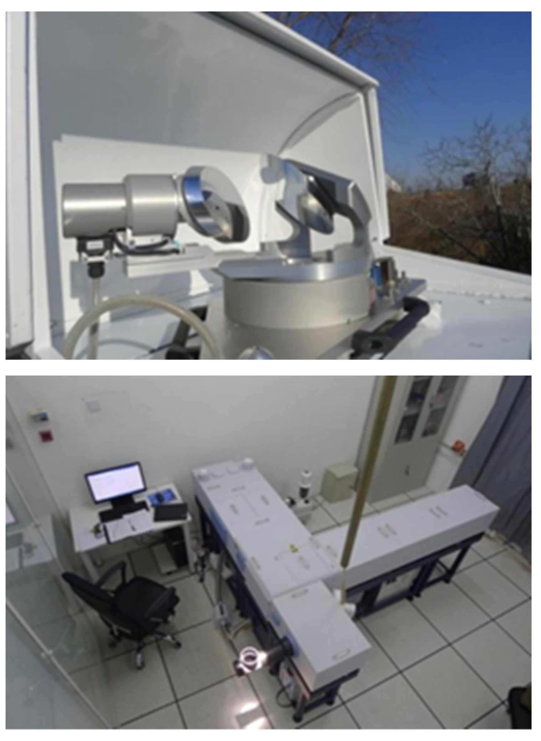
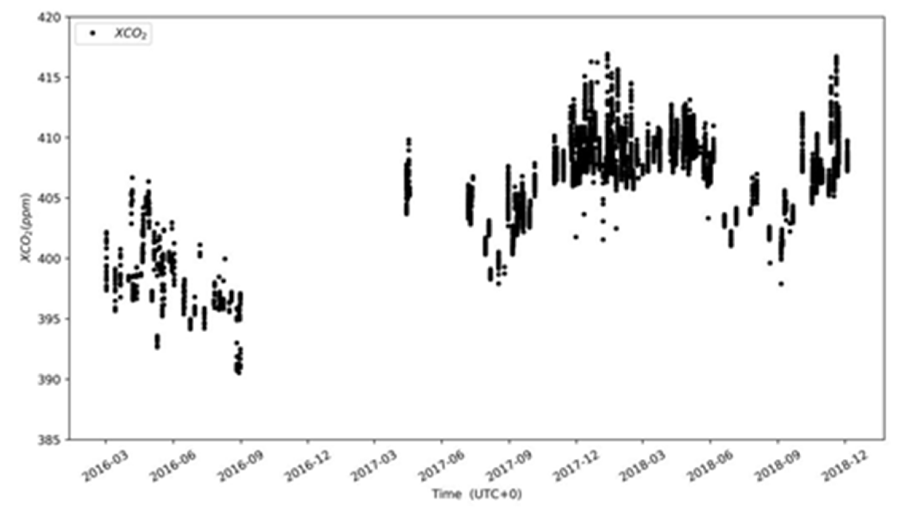
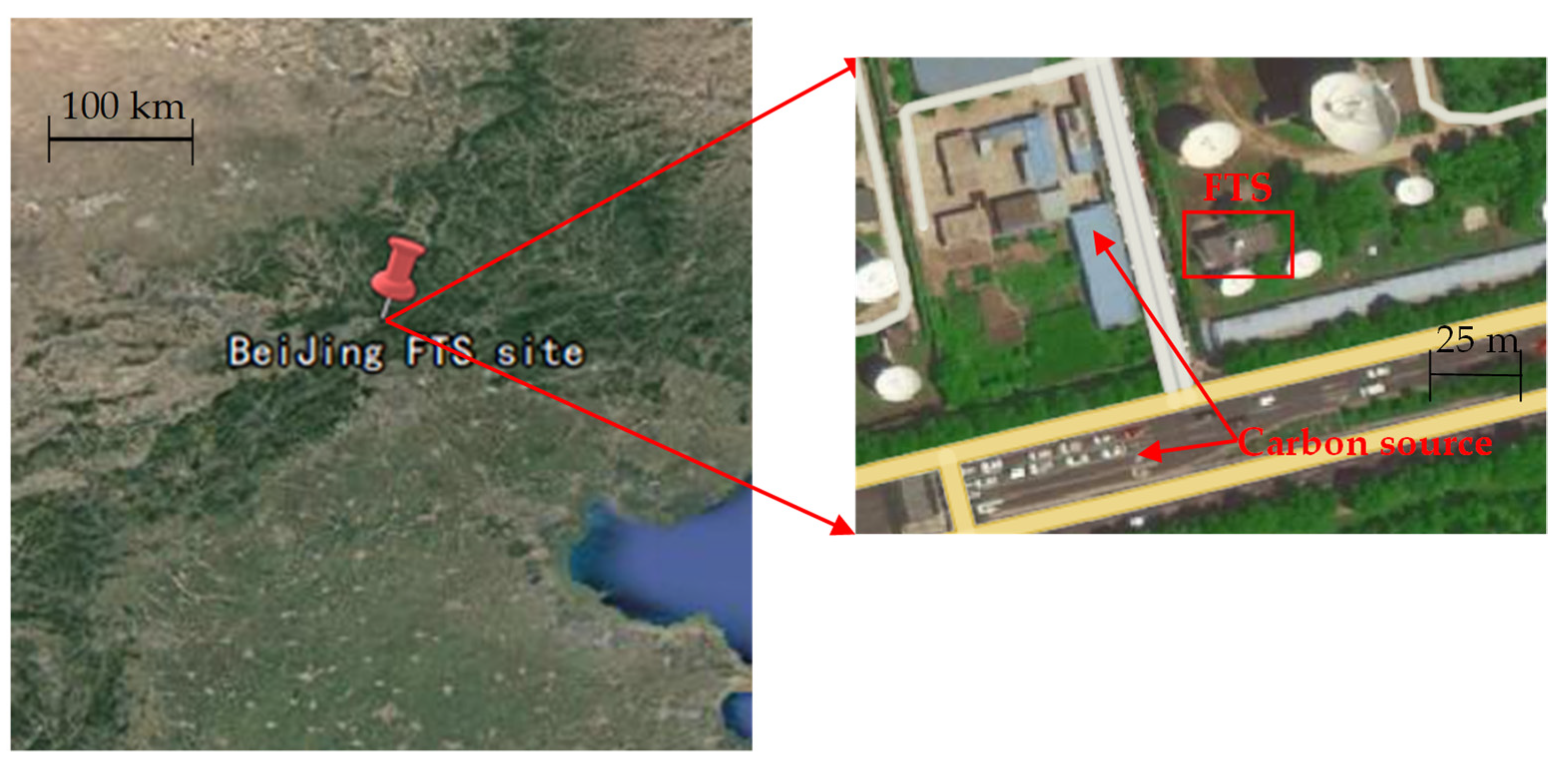
2.1. Site FTS Measurements and Retrieval Method
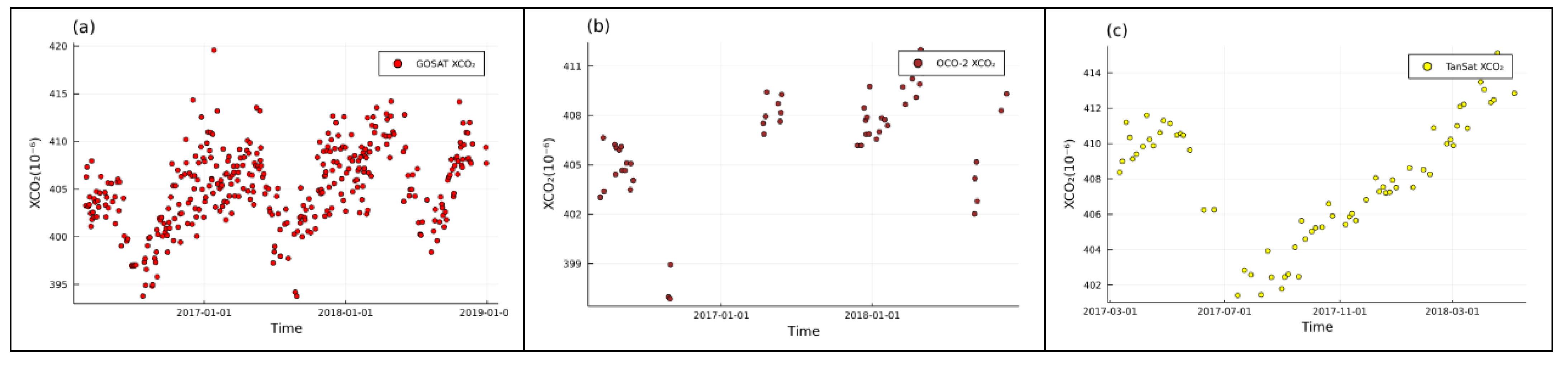
2.2. Satellite Data
2.2.1. GOSAT Data
2.2.2. OCO-2 Data
2.2.3. TanSat Data
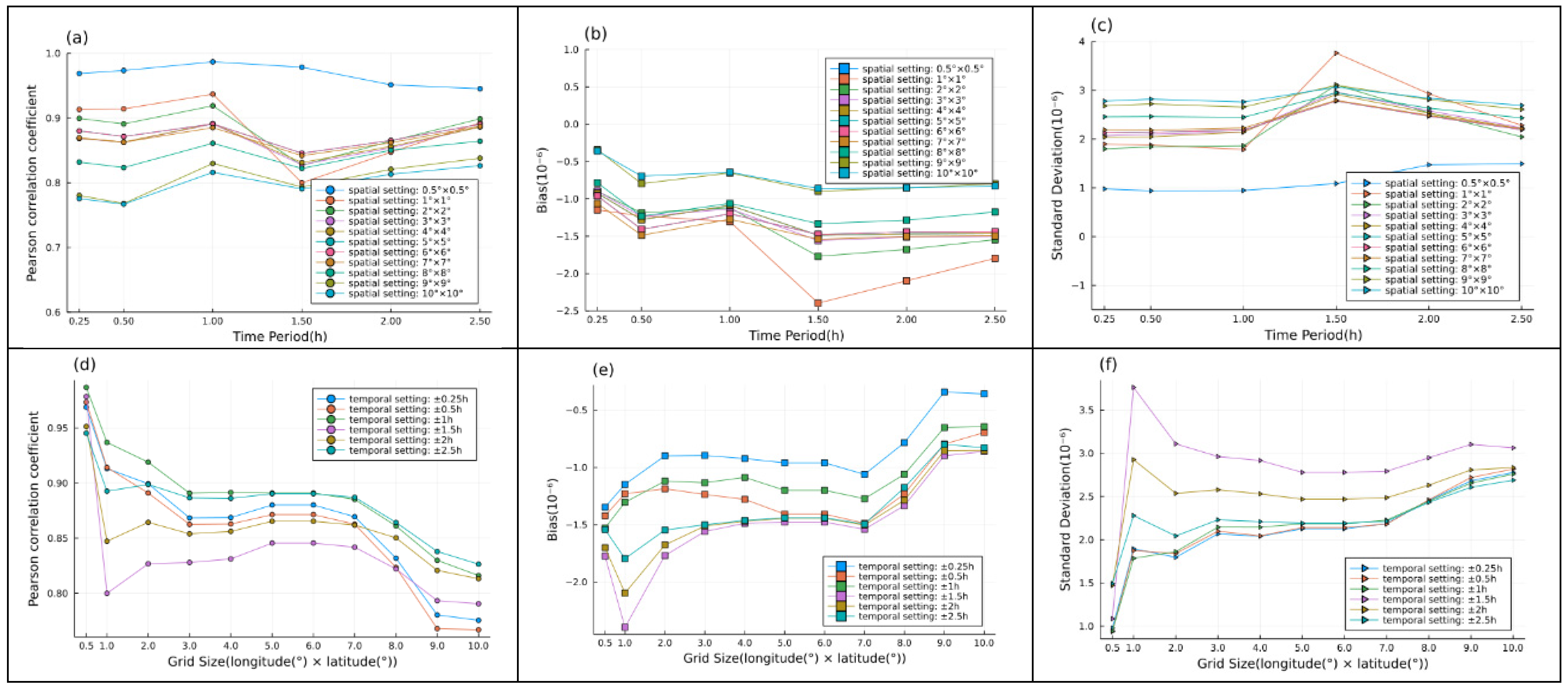
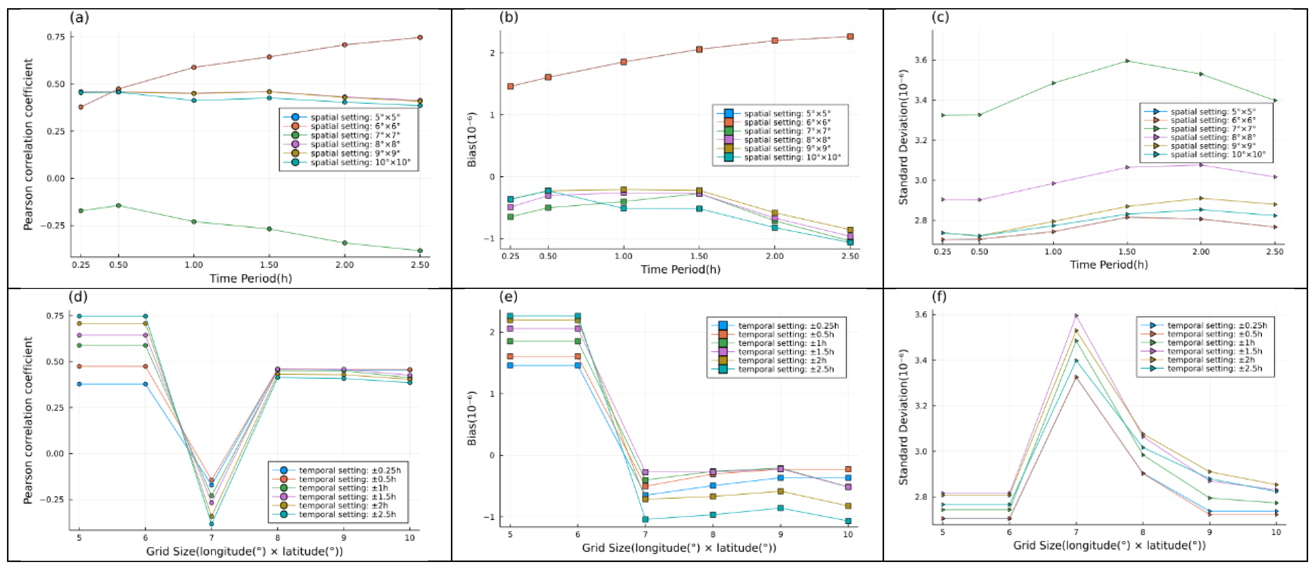
2.3. Methods
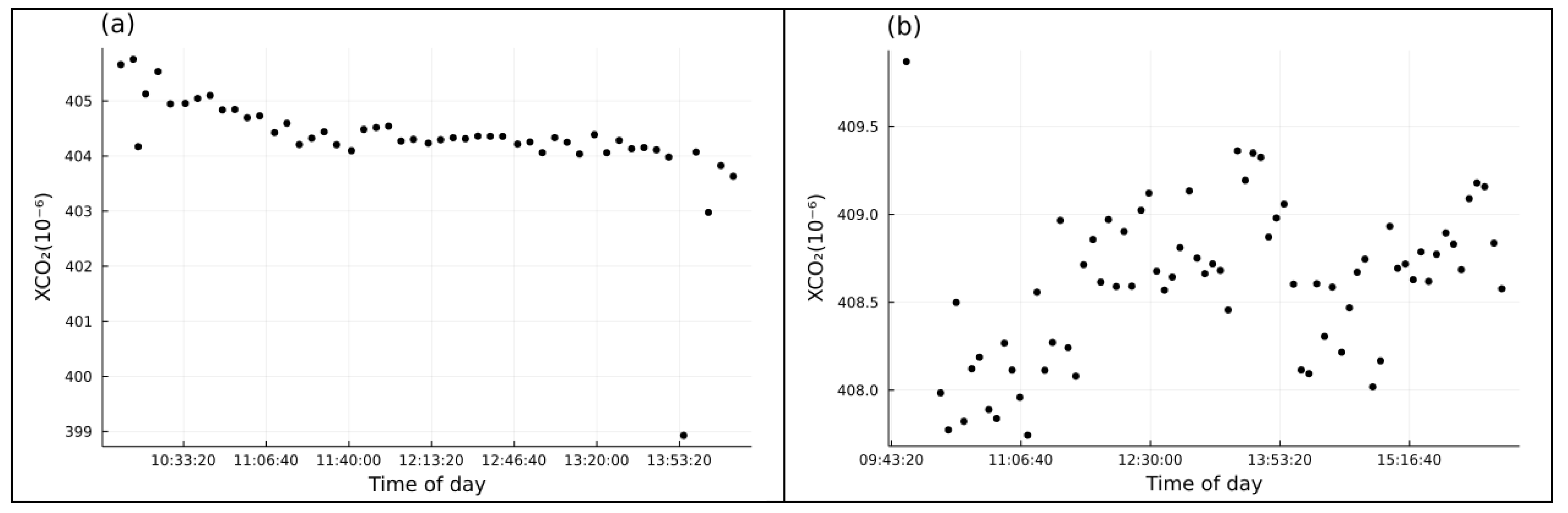
3. Results
4. Discussion
Author Contributions
Funding
Institutional Review Board Statement
Informed Consent Statement
Data Availability Statement
Acknowledgments
Conflicts of Interest
References
- Josep, G.; Canadell, J.G.; Monteiro, P.M.S.; Costa, M.H.; Cotrim da Cunha, L.; Cox, P.M.; Eliseev, A.V.; Henson, S.; Ishii, M.; Jaccard, S.; et al. Global Carbon and other Biogeochemical Cycles and Feedbacks. In Climate Change 2021: The Physical Science Basis. Contribution of Working Group I to the Sixth Assessment Report of the Intergovernmental Panel on Climate Change; Masson-Delmotte, V., Zhai, P., Pirani, A., Connors, S.L., Péan, C., Berger, S., Caud, N., Chen, Y., Goldfarb, L., Gomis, M.I., et al., Eds.; Cambridge University Press: Cambridge, UK, 2021; in press. [Google Scholar]
- WMO. WMO Greenhouse Gas Bulletin (GHG Bulletin)—No.17: The State of Greenhouse Gases in the Atmosphere Based on Global Observations through 2020. 2021. Available online: https://public.wmo.int/en/media/press-release/greenhouse-gas-bulletin-another-year-another-record (accessed on 10 November 2021).
- Krings, T.; Neininger, B.; Gerilowski, K.; Krautwurst, S.; Buchwitz, M.; Burrows, J.P.; Lindemann, C.; Ruhtz, T.; Schüttemeyer, D.; Bovensmann, H. Airborne remote sensing and in situ measurements of atmospheric CO2 to quantify point source emissions. Atmos. Meas. Tech. 2018, 11, 721–739. [Google Scholar] [CrossRef] [Green Version]
- Chevallier, F. Impact of correlated observation errors on inverted CO2 surface fluxes from OCO measurements. Geophys. Res. Lett. 2007, 34. [Google Scholar] [CrossRef]
- Rayner, P.J.; O’Brien, D.M. The utility of remotely sensed CO2 concentration data in surface source inversions. Geophys. Res. Lett. 2001, 28, 175–178. [Google Scholar] [CrossRef] [Green Version]
- Feng, L.; Palmer, P.I.; Bösch, H.; Parker, R.J.; Webb, A.J.; Correia, C.S.C.; Deutscher, N.M.; Domingues, L.G.; Feist, D.G.; Gatti, L.V.; et al. Consistent regional fluxes of CH4 and CO2 inferred from GOSAT proxy XCH4: XCO2 retrievals, 2010–2014. Atmos. Chem. Phys. 2017, 17, 4781–4797. [Google Scholar] [CrossRef] [Green Version]
- Bovensmann, H.; Buchwitz, M.; Burrows, J.P.; Reuter, M.; Krings, T.; Gerilowski, K.; Schneising, O.; Heymann, J.; Tretner, A.; Erzinger, J. A remote sensing technique for global monitoring of power plant CO2 emissions from space and related applications. Atmos. Meas. Tech. 2010, 3, 781–811. [Google Scholar] [CrossRef] [Green Version]
- Pagano, T.S.; Picard, R.H.; Chahine, M.T.; Schäfer, K.; Comeron, A.; Fetzer, E.J.; van Weele, M. The Atmospheric Infrared Sounder (AIRS) on the NASA Aqua Spacecraft: A general remote sensing tool for understanding atmospheric structure, dynamics, and composition. In Proceedings of the Remote Sensing of Clouds and the Atmosphere XV, Toulouse, France, 21–23 September 2010. [Google Scholar]
- Beer, R. TES on the aura mission: Scientific objectives, measurements, and analysis overview. IEEE Trans. Geosci. Remote Sens. 2006, 44, 1102–1105. [Google Scholar] [CrossRef]
- Goldberg, M.D.; Blumstein, D.; Bloom, H.J.; Tournier, B.; Cayla, F.R.; Huang, A.H.; Ardanuy, P.E.; Phulpin, T.; Fjortoft, R.; Buil, C.; et al. In-flight performance of the infrared atmospheric sounding interferometer (IASI) on METOP-A. In Proceedings of the Atmospheric and Environmental Remote Sensing Data Processing and Utilization III: Readiness for GEOSS, San Diego, CA, USA, 27–28, 30 August 2007. [Google Scholar]
- Wang, J.S.; Kawa, S.R.; Collatz, G.J.; Sasakawa, M.; Gatti, L.V.; Machida, T.; Liu, Y.; Manyin, M.E. A Global Synthesis Inversion Analysis of Recent Variability in CO2 Fluxes Using GOSAT and In Situ Observations. Atmos. Chem. Phys. 2018, 18, 11097–11124. [Google Scholar] [CrossRef] [Green Version]
- Basu, S.; Baker, D.F.; Chevallier, F.; Patra, P.K.; Liu, J.; Miller, J.B. The impact of transport model differences on CO2 surface flux estimates from OCO-2 retrievals of column average CO2. Atmos. Chem. Phys. 2018, 18, 7189–7215. [Google Scholar] [CrossRef] [Green Version]
- Yang, D.; Liu, Y.; Feng, L.; Wang, J.; Yao, L.; Cai, Z.; Zhu, S.; Lu, N.; Lyu, D. The First Global Carbon Dioxide Flux Map Derived from TanSat Measurements. Adv. Atmos. Sci. 2021, 38, 1433–1443. [Google Scholar] [CrossRef]
- Butler, J.J.; Xiong, X.; Gu, X.; Crisp, D. Measuring atmospheric carbon dioxide from space with the Orbiting Carbon Observatory-2 (OCO-2). In Proceedings of the Earth Observing Systems XX, San Diego, CA, USA, 9–13 August; 2015. [Google Scholar]
- Ran, Y.; Li, X. TanSat: A new star in global carbon monitoring from China. Sci. Bull. 2019, 64, 284–285. [Google Scholar] [CrossRef] [Green Version]
- Taylor, T.E.; Eldering, A.; Merrelli, A.; Kiel, M.; Somkuti, P.; Cheng, C.; Rosenberg, R.; Fisher, B.; Crisp, D.; Basilio, R.; et al. OCO-3 early mission operations and initial (vEarly) XCO2 and SIF retrievals. Remote Sens. Environ. 2020, 251, 112032. [Google Scholar] [CrossRef]
- Li, Z.Q.; Xie, Y.S.; Gu, X.F.; Li, D.H.; Li, K.T.; Zhang, X.Y.; Wu, J.; Xiong, W. Atmospheric column CO2 measurement from a new automatic ground-based sun photometer in Beijing from 2010 to 2012. Atmos. Meas. Tech. Discuss. 2012, 5, 8313–8341. [Google Scholar] [CrossRef]
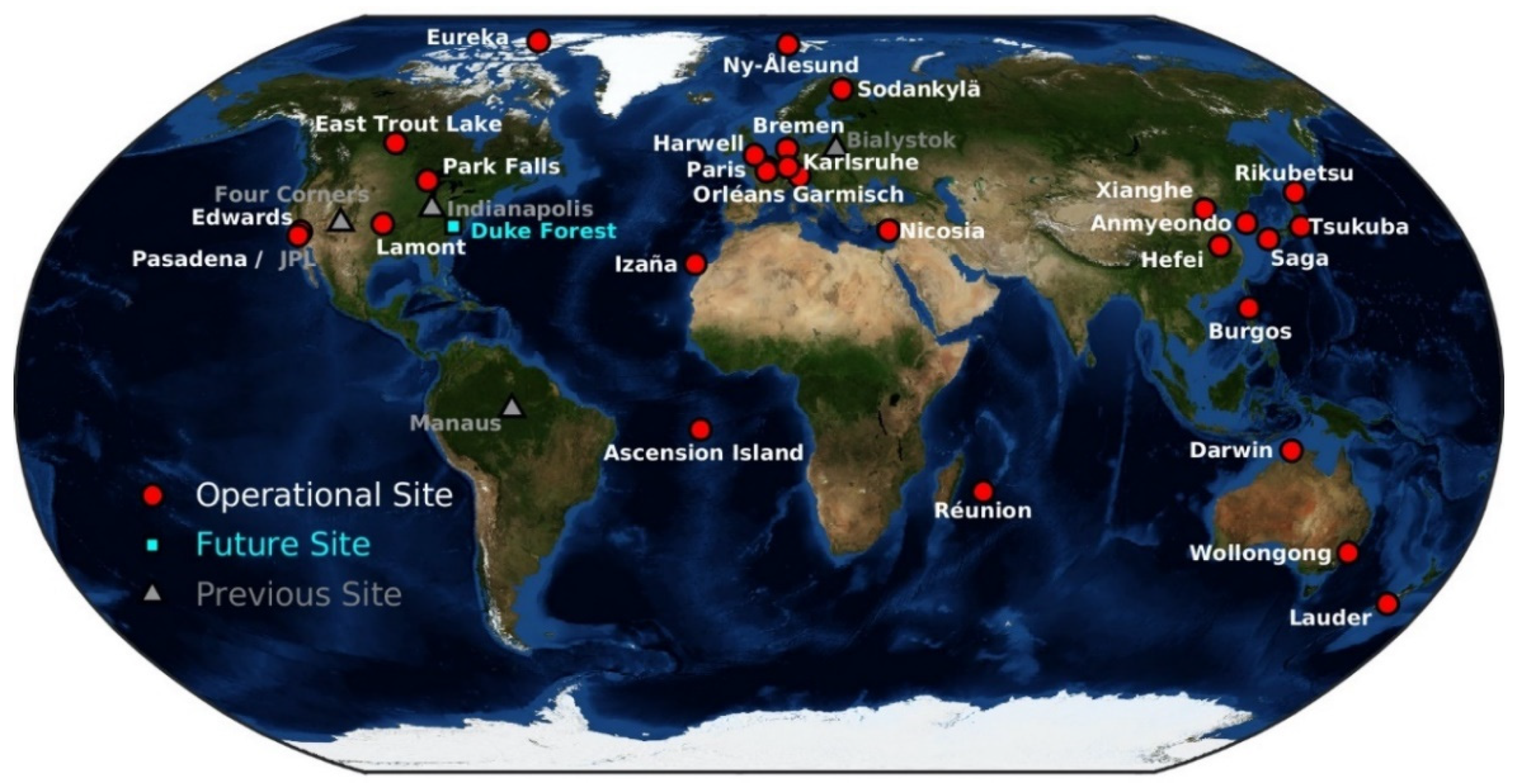
- Wunch, D.; Toon, G.C.; Blavier, J.F.; Washenfelder, R.A.; Notholt, J.; Connor, B.J.; Griffith, D.W.; Sherlock, V.; Wennberg, P.O. The total carbon column observing network. Philos. Trans. A Math. Phys. Eng. Sci. 2011, 369, 2087–2112. [Google Scholar] [CrossRef] [Green Version]
- Morino, I.; Uchino, O.; Inoue, M.; Yoshida, Y.; Yokota, T.; Wennberg, P.O.; Toon, G.C.; Wunch, D.; Roehl, C.M.; Notholt, J.; et al. Preliminary validation of column-averaged volume mixing ratios of carbon dioxide and methane retrieved from GOSAT short-wavelength infrared spectra. Atmos. Meas. Tech. Discuss. 2010, 3, 5613–5643. [Google Scholar] [CrossRef] [Green Version]
- Cogan, A.J.; Boesch, H.; Parker, R.J.; Feng, L.; Palmer, P.I.; Blavier, J.F.L.; Deutscher, N.M.; Macatangay, R.; Notholt, J.; Roehl, C.; et al. Atmospheric carbon dioxide retrieved from the Greenhouse gases Observing SATellite (GOSAT): Comparison with ground-based TCCON observations and GEOS-Chem model calculations. J. Geophys. Res. Atmos. 2012, 117, 21. [Google Scholar] [CrossRef] [Green Version]
- Oshchepkov, S.; Bril, A.; Yokota, T.; Morino, I.; Yoshida, Y.; Matsunaga, T.; Belikov, D.; Wunch, D.; Wennberg, P.; Toon, G.; et al. Effects of atmospheric light scattering on spectroscopic observations of greenhouse gases from space: Validation of PPDF-based CO2 retrievals from GOSAT. J. Geophys. Res. Atmos. 2012, 117, 12. [Google Scholar] [CrossRef] [Green Version]
- Oshchepkov, S.; Bril, A.; Yokota, T.; Wennberg, P.O.; Deutscher, N.M.; Wunch, D.; Toon, G.C.; Yoshida, Y.; O’Dell, C.W.; Crisp, D.; et al. Effects of atmospheric light scattering on spectroscopic observations of greenhouse gases from space. Part 2: Algorithm intercomparison in the GOSAT data processing for CO2 retrievals over TCCON sites. J. Geophys. Res. Atmos. 2013, 118, 1493–1512. [Google Scholar] [CrossRef] [Green Version]
- Yoshida, Y.; Kikuchi, N.; Morino, I.; Uchino, O.; Oshchepkov, S.; Bril, A.; Saeki, T.; Schutgens, N.; Toon, G.C.; Wunch, D.; et al. Improvement of the retrieval algorithm for GOSAT SWIR XCO2 and XCH4 and their validation using TCCON data. Atmos. Meas. Tech. 2013, 6, 1533–1547. [Google Scholar] [CrossRef]
- Nguyen, H.; Osterman, G.; Wunch, D.; O’Dell, C.; Mandrake, L.; Wennberg, P.; Fisher, B.; Castano, R. A method for colocating satellite XCO2 data to ground-based data and its application to ACOS-GOSAT and TCCON. Atmos. Meas. Tech. Discuss. 2014, 7, 2631–2644. [Google Scholar] [CrossRef] [Green Version]
- Zhang, M.; Zhang, X.-Y.; Liu, R.-X.; Hu, L.-Q. A study of the validation of atmospheric CO2 from satellite hyper spectral remote sensing. Adv. Clim. Chang. Res. 2014, 5, 131–135. [Google Scholar] [CrossRef]
- Zhou, M.; Zhang, X.; Wang, P.; Wang, S.; Guo, L.; Hu, L. XCO2 satellite retrieval experiments in short-wave infrared spectrum and ground-based validation. Sci. China Earth Sci. 2015, 58, 1191–1197. [Google Scholar] [CrossRef]
- Deng, A.; Yu, T.; Cheng, T.; Gu, X.; Zheng, F.; Guo, H. Intercomparison of Carbon Dioxide Products Retrieved from GOSAT Short-Wavelength Infrared Spectra for Three Years (2010–2012). Atmosphere 2016, 7, 109. [Google Scholar] [CrossRef] [Green Version]
- Inoue, M.; Morino, I.; Uchino, O.; Nakatsuru, T.; Yoshida, Y.; Yokota, T.; Wunch, D.; Wennberg, P.O.; Roehl, C.M.; Griffith, D.W.T.; et al. Bias corrections of GOSAT SWIR XCO2 and XCH4 with TCCON data and their evaluation using aircraft measurement data. Atmos. Meas. Tech. 2016, 9, 3491–3512. [Google Scholar] [CrossRef] [Green Version]
- Kulawik, S.; Wunch, D.; O’Dell, C.; Frankenberg, C.; Reuter, M.; Oda, T.; Chevallier, F.; Sherlock, V.; Buchwitz, M.; Osterman, G.; et al. Consistent evaluation of ACOS-GOSAT, BESD-SCIAMACHY, CarbonTracker, and MACC through comparisons to TCCON. Atmos. Meas. Tech. 2016, 9, 683–709. [Google Scholar] [CrossRef] [Green Version]
- Bi, Y.; Wang, Q.; Yang, Z.; Chen, J.; Bai, W. Validation of Column-Averaged Dry-Air Mole Fraction of CO2 Retrieved from OCO-2 Using Ground-Based FTS Measurements. J. Meteorol. Res. 2018, 32, 433–443. [Google Scholar] [CrossRef]
- Wang, S.; van der A, R.J.; Stammes, P.; Wang, W.; Zhang, P.; Lu, N.; Zhang, X.; Bi, Y.; Wang, P.; Fang, L. Carbon Dioxide Retrieval from TanSat Observations and Validation with TCCON Measurements. Remote Sens. 2020, 12, 2204. [Google Scholar] [CrossRef]
- Toon, G.; Sen, B.; Blavier, J.F.; Sasano, Y.; Yokota, T.; Kanzawa, H.; Ogawa, T.; Suzuki, M.; Shibasaki, K. Comparison of ILAS and MkIV profiles of atmospheric trace gases measured above Alaska in May 1997. J. Geophys. Res. Atmos. 2002, 107, ILS 8-1–ILS 8-6. [Google Scholar] [CrossRef]
- Connor, B.J.; Sherlock, V.; Toon, G.; Wunch, D.; Wennberg, P.O. GFIT2: An experimental algorithm for vertical profile retrieval from near-IR spectra. Atmos. Meas. Tech. 2016, 9, 3513–3525. [Google Scholar] [CrossRef] [Green Version]
- Yokota, T.; Yoshida, Y.; Eguchi, N.; Ota, Y.; Tanaka, H.; Watanabe, H.; Maksyutov, S. Global Concentrations of CO2 and CH4 Retrieved from GOSAT: First Preliminary Results. Sci. Online Lett. Atmos. Sola 2009, 5, 160–163. [Google Scholar] [CrossRef] [Green Version]
- Kuze, A.; Suto, H.; Nakajima, M.; Hamazaki, T. Thermal and near infrared sensor for carbon observation Fourier-transform spectrometer on the Greenhouse Gases Observing Satellite for greenhouse gases monitoring. Appl. Opt. 2009, 48, 6716–6733. [Google Scholar] [CrossRef]
- Rastogi, B.; Miller, J.B.; Trudeau, M.; Andrews, A.E.; Hu, L.; Mountain, M.; Nehrkorn, T.; Baier, B.; McKain, K.; Mund, J.; et al. Evaluating consistency between total column CO2 retrievals from OCO-2 and the in situ network over North America: Implications for carbon flux estimation. Atmos. Chem. Phys. 2021, 21, 14385–14401. [Google Scholar] [CrossRef]
- Meynart, R.; Pollock, R.; Neeck, S.P.; Haring, R.E.; Holden, J.R.; Shimoda, H.; Johnson, D.L.; Kapitanoff, A.; Mohlman, D.; Phillips, C.; et al. The Orbiting Carbon Observatory instrument: Performance of the OCO instrument and plans for the OCO-2 instrument. In Proceedings of the SPIE—The International Society for Optical Engineering, Toulouse, France, 20–23 September 2010; Volume 7826. [Google Scholar] [CrossRef]
- O’Dell, C.W.; Connor, B.; Bösch, H.; O’ Brien, D.; Frankenberg, C.; Castano, R.; Christi, M.; Eldering, D.; Fisher, B.; Gunson, M.; et al. The ACOS CO2 retrieval algorithm—Part 1: Description and validation against synthetic observations. Atmos. Meas. Tech. 2012, 5, 99–121. [Google Scholar] [CrossRef] [Green Version]
- O’Dell, C.W.; Eldering, A.; Wennberg, P.O.; Crisp, D.; Gunson, M.R.; Fisher, B.; Frankenberg, C.; Kiel, M.; Lindqvist, H.; Mandrake, L.; et al. Improved retrievals of carbon dioxide from Orbiting Carbon Observatory-2 with the version 8 ACOS algorithm. Atmos. Meas. Tech. 2018, 11, 6539–6576. [Google Scholar] [CrossRef] [Green Version]
- Kiel, M.; O’Dell, C.W.; Fisher, B.; Eldering, A.; Nassar, R.; MacDonald, C.G.; Wennberg, P.O. How bias correction goes wrong: Measurement of XCO2 affected by erroneous surface pressure estimates. Atmos. Meas. Tech. 2019, 12, 2241–2259. [Google Scholar] [CrossRef] [Green Version]
- Wang, X.; Guo, Z.; Huang, Y.; Fan, H.; Li, W. A cloud detection scheme for the Chinese Carbon Dioxide Observation Satellite (TANSAT). Adv. Atmos. Sci. 2016, 34, 16–25. [Google Scholar] [CrossRef] [Green Version]
- Yang, D.; Liu, Y.; Boesch, H.; Yao, L.; Di Noia, A.; Cai, Z.; Lu, N.; Lyu, D.; Wang, M.; Wang, J.; et al. A New TanSat XCO2 Global Product towards Climate Studies. Adv. Atmos. Sci. 2020, 38, 8–11. [Google Scholar] [CrossRef]
- Liu, Y.; Yang, D.; Cai, Z. A retrieval algorithm for TanSat XCO2 observation: Retrieval experiments using GOSAT data. Chin. Sci. Bull. 2013, 58, 1520–1523. [Google Scholar] [CrossRef] [Green Version]
- Bao, Z.; Zhang, X.; Yue, T.; Zhang, L.; Wang, Z.; Jiao, Y.; Bai, W.; Meng, X. Retrieval and Validation of XCO2 from TanSat Target Mode Observations in Beijing. Remote Sens. 2020, 12, 3063. [Google Scholar] [CrossRef]
- Velazco, V.A.; Deutscher, N.M.; Morino, I.; Uchino, O.; Bukosa, B.; Ajiro, M.; Kamei, A.; Jones, N.B.; Paton-Walsh, C.; Griffith, D.W.T. Satellite and ground-based measurements of XCO2 in a remote semiarid region of Australia. Earth Syst. Sci. Data 2019, 11, 935–946. [Google Scholar] [CrossRef] [Green Version]
- Wunch, D.; Wennberg, P.O.; Osterman, G.; Fisher, B.; Naylor, B.; Roehl, C.M.; O’Dell, C.; Mandrake, L.; Viatte, C.; Kiel, M.; et al. Comparisons of the Orbiting Carbon Observatory-2 (OCO-2) XCO2 measurements with TCCON. Atmos. Meas. Tech. 2017, 10, 2209–2238. [Google Scholar] [CrossRef] [Green Version]
- Kiel, M.; Eldering, A.; Roten, D.D.; Lin, J.C.; Feng, S.; Lei, R.; Lauvaux, T.; Oda, T.; Roehl, C.M.; Blavier, J.-F.; et al. Urban-focused satellite CO2 observations from the Orbiting Carbon Observatory-3: A first look at the Los Angeles megacity. Remote Sens. Environ. 2021, 258, 112314. [Google Scholar] [CrossRef]
- Newman, S.; Jeong, S.; Fischer, M.L.; Xu, X.; Haman, C.L.; Lefer, B.; Alvarez, S.; Rappenglueck, B.; Kort, E.A.; Andrews, A.E.; et al. Diurnal tracking of anthropogenic CO2 emissions in the Los Angeles basin megacity during spring 2010. Atmos. Chem. Phys. 2013, 13, 4359–4372. [Google Scholar] [CrossRef] [Green Version]


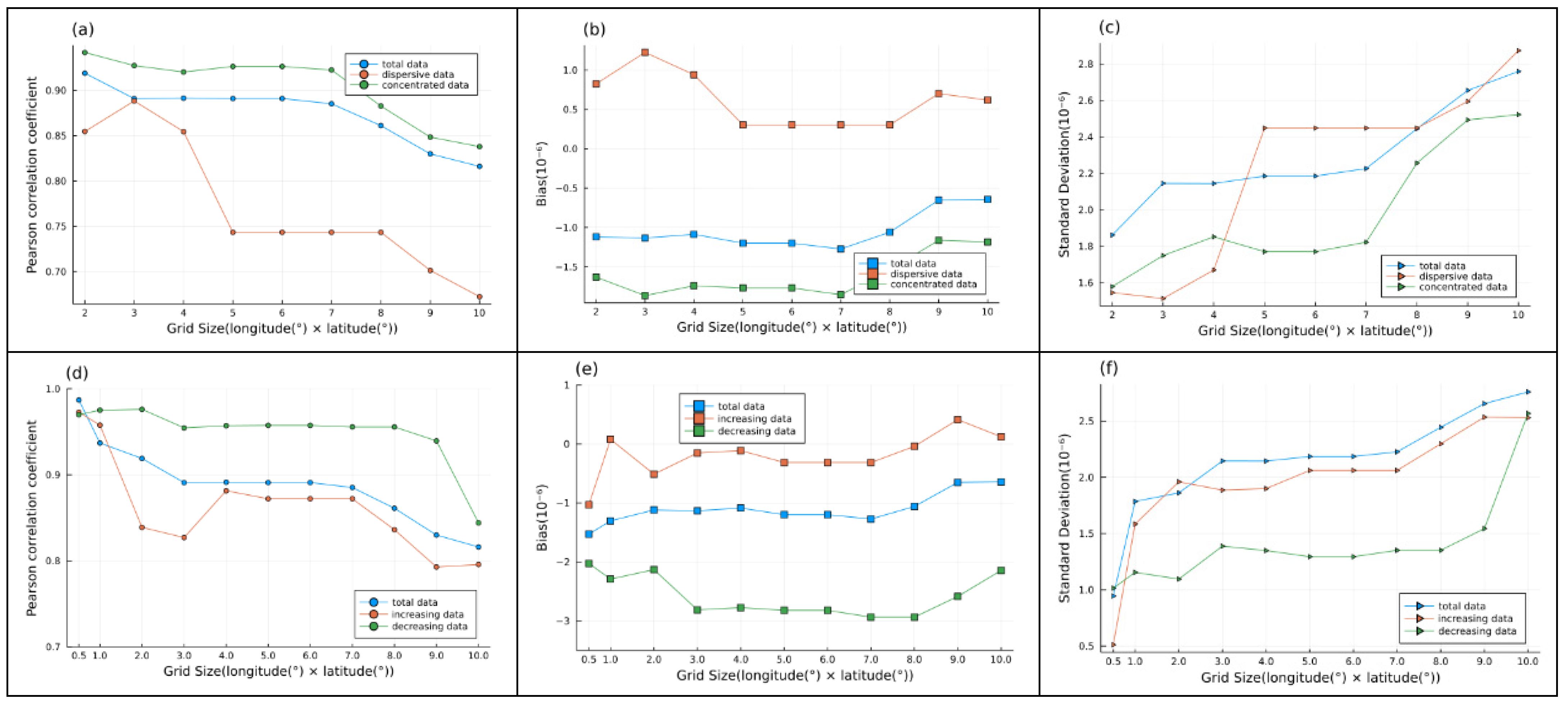
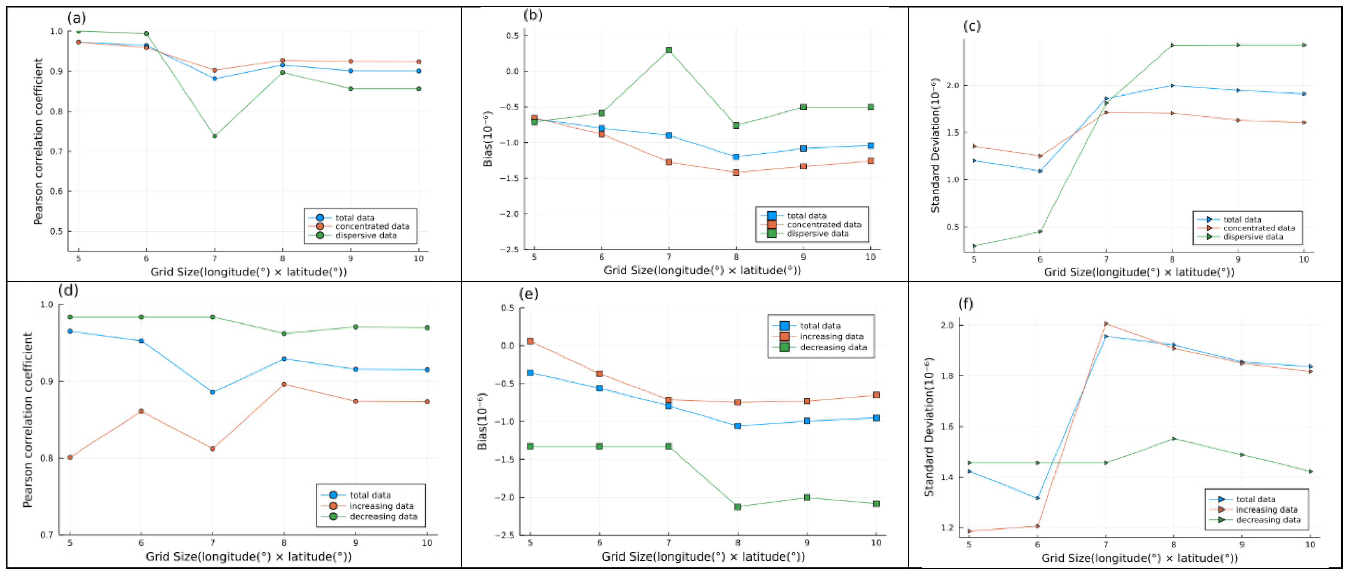
| Classification | Increasing | Decreasing | Concentrated | Dispersive |
|---|---|---|---|---|
| Number | 133 | 69 | 129 | 73 |
Publisher’s Note: MDPI stays neutral with regard to jurisdictional claims in published maps and institutional affiliations. |
© 2021 by the authors. Licensee MDPI, Basel, Switzerland. This article is an open access article distributed under the terms and conditions of the Creative Commons Attribution (CC BY) license (https://creativecommons.org/licenses/by/4.0/).
Share and Cite
Yang, S.; Meng, X.; Zhang, X.; Zhang, L.; Bai, W.; Yang, Z.; Zhang, P.; Deng, Z.; Zhang, X.; Cao, X. Study on the Ground-Based FTS Measurements at Beijing, China and the Colocation Sensitivity of Satellite Data. Atmosphere 2021, 12, 1586. https://doi.org/10.3390/atmos12121586
Yang S, Meng X, Zhang X, Zhang L, Bai W, Yang Z, Zhang P, Deng Z, Zhang X, Cao X. Study on the Ground-Based FTS Measurements at Beijing, China and the Colocation Sensitivity of Satellite Data. Atmosphere. 2021; 12(12):1586. https://doi.org/10.3390/atmos12121586
Chicago/Turabian StyleYang, Sen, Xiaoyang Meng, Xingying Zhang, Lu Zhang, Wenguang Bai, Zhongdong Yang, Peng Zhang, Zhili Deng, Xin Zhang, and Xifeng Cao. 2021. "Study on the Ground-Based FTS Measurements at Beijing, China and the Colocation Sensitivity of Satellite Data" Atmosphere 12, no. 12: 1586. https://doi.org/10.3390/atmos12121586