Radiometric Method for Determining Canopy Stomatal Conductance in Controlled Environments


1
AECOM, Air Revitalization Lab, Mail code: LASSO-008, Kennedy Space Center, Merritt Island, FL 32899, USA
2
Plants, Soils and Biometeorology Department, Utah State University, Logan, UT 84322, USA
*
Author to whom correspondence should be addressed.
Agronomy 2019, 9(3), 114; https://doi.org/10.3390/agronomy9030114
Submission received: 1 January 2019
/
Revised: 19 February 2019
/
Accepted: 20 February 2019
/
Published: 27 February 2019
(This article belongs to the Special Issue Crop Evapotranspiration)
Abstract
:Canopy stomatal conductance is a key physiological factor controlling transpiration from plant canopies, but it is extremely difficult to determine in field environments. The objective of this study was to develop a radiometric method for calculating canopy stomatal conductance for two plant species—wheat and soybean from direct measurements of bulk surface conductance to water vapor and the canopy aerodynamic conductance in controlled-environment chambers. The chamber provides constant net radiation, temperature, humidity, and ventilation rate to the plant canopy. In this method, stepwise changes in chamber CO2 alter canopy temperature, latent heat, and sensible heat fluxes simultaneously. Sensible heat and the radiometric canopy-to-air temperature difference are computed from direct measurements of net radiation, canopy transpiration, photosynthesis, radiometric temperature, and air temperature. The canopy aerodynamic conductance to the transfer of water vapor is then determined from a plot of sensible heat versus radiometric canopy-to-air temperature difference. Finally, canopy stomatal conductance is calculated from canopy surface and aerodynamic conductances. The canopy aerodynamic conductance was 5.5 mol m−2 s−1 in wheat and 2.5 mol m−2 s−1 in soybean canopies. At 400 umol mol−1 of CO2 and 86 kPa atmospheric pressure, canopy stomatal conductances were 2.1 mol m−2 s−1 for wheat and 1.1 mol m−2 s−1 for soybean, comparable to canopy stomatal conductances reported in field studies. This method measures canopy aerodynamic conductance in controlled-environment chambers where the log-wind profile approximation does not apply and provides an improved technique for measuring canopy-level responses of canopy stomatal conductance and the decoupling coefficient. The method was used to determine the response of canopy stomatal conductance to increased CO2 concentration and to determine the sensitivity of canopy transpiration to changes in canopy stomatal conductance. These responses are useful for improving the prediction of ecosystem-level water fluxes in response to climatic variables.
1. Introduction
Understanding boundary layer and land surface feedbacks on canopy transpiration is essential for developing simpler and realistic climate change models and for improving the prediction of ecosystem-level water fluxes in response to climatic variables [1,2]. Canopy stomatal conductance (GS), a key physiological factor controlling transpiration from plant stands, is an important component of land surface feedbacks because it regulates evapotranspiration and surface temperature changes in response to incident radiation, CO2 concentration, and vapor pressure deficit (VPD). This regulatory function is reflected in canopy temperature, which in turn, determines the magnitude and direction of sensible heat exchange between the vegetation and its environment. At regional scales, stomata exert little control, and daily transpiration of well-watered vegetation is predominantly controlled by radiation and temperature [3,4,5], in part due to feedbacks that cannot be predicted from single leaf measurements alone [3]. Since canopy-scale transpiration is determined by the ratio between canopy aerodynamic conductance (gA) and GS [4,6,7], improved methods for measuring gA, as well as measuring responses of GS to environmental variables (e.g., light, CO2, VPD, soil moisture, and temperature), are needed for studying the processes controlling feedback and stomatal control of evaporation from regional land surfaces.
In the field, gA is often approximated by the conductance to momentum transfer determined using the log-wind profile approximation, which requires at least 100 m of fetch and thus cannot be used in controlled-environment chambers [8]. In controlled environments, leaf boundary conductance has been estimated from measurements with wet filter paper analogs [9], from cooling curves of metal models of leaves [10], or from combined energy balance and temperature measurements using metal leaf models [11,12]. However, Jarvis and McNaughton [3] argue that leaf level measurements of stomatal control of transpiration may not be applicable to plant canopies in the field because the amount of ventilation in leaf cuvettes and plant chambers typically prevents feedback between transpiration and VPD observed in the field.
GS can be derived using energy balance approaches from canopy surface conductance to water vapor (GSFC), latent heat flux (LE), and the VPD at the leaf surface (Ds). Similarly, the single-layer or “big leaf” GS may be computed from GSFC, provided the boundary layer conductance to water vapor (i.e., gA) and the mean aerodynamic canopy temperature (TAero) are known [13,14]. In the field, GSFC is calculated from canopy-level LE obtained using lysimeters, Bowen ratio, and eddy correlation systems [15], or by inverting the Penman–Monteith equation [13]. However, these approaches for measuring canopy-level LE do not permit partitioning of transpiration among individual species and often cannot distinguish between transpiration and evaporation from the soil or from wet leaf surfaces. Thus, GSFC is not always related to estimates of canopy GS derived from single leaf measurements because it often includes significant contributions from soil evaporation [13].
Smith et al. [16] used canopy-level energy balance measurements to estimate sensible heat flux (H) of a wheat field from radiometric canopy temperature when canopy gA and LE were known. Their approach produced accurate estimates of hourly LE, which suggests that gA could be estimated if H and the canopy-to-air temperature difference are measured accurately. However, canopy gA determined from changes in radiometric canopy temperature differs from gA determined using the log-wind profile approximation because it includes the conductance to heat and water vapor across leaf boundary layers, as well as the turbulent conductance caused by the movement of air eddies between the canopy and the atmosphere [17,18].
Canopy GS obtained from energy balance approaches may contain considerable errors because Ds and LE are estimated using measurements of canopy radiometric temperature (TR) to approximate the aerodynamic canopy temperature [19,20,21]. In the field, estimating TAero from infrared measurements is complicated because radiometric measurements depend on the view angle of the sensor, sun angle, degree of crop cover, spatial variability of canopy emissivity, and atmospheric attenuation, and they often include significant temperature contributions from soil surfaces [20,22,23,24,25]. A systematic difference of −1 °C was measured between radiometric and aerodynamic temperatures by Huband and Monteith [26], although differences ranging from 2 to 6 °C have also been observed [13]. The difference between TAero and TR can be very small in dense canopies, but it can exceed 10 °C in sparse vegetation because of contributions from soil temperature ([18,27]. These differences are significant because small errors of −1 °C in the surface-to-air temperature difference can represent an uncertainty in latent heat fluxes of ~40 W m−2 [13]. Many complicating factors that affect infrared measurements of canopy temperature in field settings can be minimized in controlled environments by using high planting density canopies grown under constant lighting. In dense canopies, canopy brightness temperature measured with infrared sensors approximates canopy radiometric temperature [28], but errors due to radiation reflected into the sensor and artifacts caused by fluctuating sensor body temperatures remain [29].
The purpose of this study was to develop a radiometric method for measuring canopy GS of well-watered plant canopies in controlled environments. The hypothesis tested was that a radiometric method utilizing canopy-level energy balance measurements provides more accurate estimates of canopy stomatal conductance than bottom-up methods scaling leaf-level to canopy-level conductance or top-down methods that estimate canopy surface conductance from field data. Bottom-up methods require that leaf area index be known and must integrate the responses of leaf stomatal conductance to vertical gradients in radiation, temperature, and humidity. Conductances from top-down methods using field data typically include significant contributions of soil evaporation, and field radiometric data include soil surface temperatures that cause significant differences between radiometric and aerodynamic temperatures [13].
Simultaneous measurements of energy balance, gas fluxes, and canopy temperature at constant environmental conditions were used to compute canopy GS from surface GSFC and canopy gA (Figure 1). The relation between radiometric and aerodynamic temperatures was studied by varying incident radiation and wind speed. Canopy GS and gA of high planting density wheat (Triticum aestivum L. cv. USU Apogee) and soybean (Glycine max L. cv. Hoyt) canopies were measured at 400 umol mol−1 CO2. The radiometric method was used to explore the effects of rising CO2 concentration on canopy GS and to describe stomatal feedbacks to transpiration using the canopy-scale decoupling coefficient.
2. Materials and Methods
2.1. Chamber System
In this study, 18–35-day-old, closed wheat and soybean canopies were used to examine various aspects of the method—energy balance responses to changes in radiation forcing, responses of vertical gradients in canopy-to-air temperature to fan speed or light level, responses in canopy-to-air temperature and sensible heat flux to CO2 concentration, etc. Each test took several days to conduct, and plant canopies of different ages were used because the logistics of growing canopies to the same age for each test was impractical. Thus, conductances observed in a vegetative 20-day-old wheat canopy may not be the same as in a reproductive 35-day-old canopy due to ontogenetic changes in canopy structure (i.e., the presence of heads). However, overall the method is robust as long as energy balance components and canopy-to-air temperature differences are measured accurately and simultaneously.
2.2. Cultural and Environmental Conditions
Wheat and soybean canopies were grown in sealed, water-cooled, controlled-environment chambers (Model EGC-13, Environmental Growth Chambers, Chagrin Falls, OH, USA). Two canopies of the same species were grown simultaneously in adjacent chambers. Wheat was seeded into lids containing a 10 mm layer of inert media (Isolite, size CG-2, Sumitomo Corp., Denver, CO, USA) at a density of 1100 plants m−2. Soybean seedlings were transplanted into closed cell foam plugs in a Styrofoam lid at a planting density of 60 plants m−2. The seedling roots grew into a recirculating hydroponic solution after germination. The hydroponic system is described in Monje and Bugbee [30].
Inside each chamber, a polished aluminum, reflective side-wall was built around the perimeter of the ~1 m2 canopy to minimize edge effects and side lighting. The incident photosynthetic photon flux (PPFo) was 1600 µmol m−2 s−1 for wheat and 750 µmol m−2 s−1 for soybean. Lighting was provided by four, 1000 W high-pressure sodium (HPS) lamps, which were adjusted with neutral density filters to achieve ±5% PPFo uniformity over the crop surface. PPFo was measured at the top of the canopy with a quantum sensor (Model LI-190SB, LI-COR, Lincoln, NE, USA), and was adjusted daily throughout the life cycle by lowering the canopy platform as the plants grew taller. Longwave radiation emitted by the lamps was removed by a 10 cm deep water filter. The filter consisted of a glass box filled with recirculating, chilled water located below the lamps. The water filter under the lamps was removed over the course of several days during tests that change surface radiation forcing by increasing incident PPFo and longwave radiation impinging on the canopy. Advective conditions existed in the chamber because the temperature control system heated the air to maintain the chamber temperature setpoint, and the canopy was exposed to a continuous flow of warm air.
Air temperature was 21.0 ± 0.3 °C, the barometric pressure was 86 ± 0.1 kPa, and chamber CO2 varied between 400 and 1400 µmol mol−1 to manipulate canopy temperature, LE and H. Relative humidity at night was 50% ± 5%. During the day, transpiration humidified the 1300 L of chamber air and daytime relative humidity was 70 ± 5%. Wheat was grown under a 20 h light/4 h dark photoperiod and soybean under a 12 h light/12 h dark photoperiod. The canopies grew in a chamber supplied with a constant temperature (TAir) and VPD of bulk air surrounding the vegetation (DBulk) as well as a constant wind speed. Thus, boundary layer forcing (TAir and DBulk) and surface layer feedbacks (chamber wind speed) were held constant, but in nature they are dictated by diurnal changes in local climate (TAir, DBulk, and wind speed).
2.3. Gas Exchange System
Each chamber used an open gas exchange system to measure canopy photosynthesis [30,31]. The open flow system ensured that humid air (~50% relative humidity) of a constant CO2 concentration (setpoint ±10 µmol mol−1) fed the chambers at flow rates between 500 and 1100 L min−1. Air mass flow (MF; mol s−1) into the chambers was measured with mass flow meters (Model 730, Sierra Instruments, Monterey, CA, USA). The gas exchange systems were modified to use a dew point hygrometer to measure the water vapor concentration of pre- and post-chamber air from which evapotranspiration was calculated. Two solid-state multiplexers (Model AM-25T, Campbell Scientific, Logan, UT, USA), each referenced to a 100 Ohm platinum resistance thermometer, were used for precision thermocouple measurements. Data acquisition and control were performed with a datalogger (Model CR-10T, Campbell Scientific, Logan, UT, USA).
Gas exchange fluxes in each chamber were measured continuously and averaged for 2 min every 8 min. Net photosynthesis, Pnet, and dark respiration rates were calculated from the difference between pre- and post-chamber CO2 concentrations (ΔCO2), multiplied by MF of air into the chambers. ΔCO2 was measured with a differential infrared gas analyzer (Model LI-6251, LI-COR, Lincoln, NE, USA). The temperature, water vapor band broadening, and dilution corrections used for the C fluxes are described in Monje and Bugbee [30]. Chamber evapotranspiration (ET) was determined from the difference in mole fraction of water vapor between pre- and post-chamber air (ΔXh20), multiplied by mass flow rate entering the chamber (ET = ΔXh20 × MF). ΔΧh20 was determined from sequential measurements of pre- and post-chamber air dewpoint made with a dewpoint hygrometer (Model Dew-10, General Eastern, Watertown, MA, USA). Air flow was changed to increase ΔCO2 and ΔΧh20 in the chamber. The flow rate of air entering the chamber was not corrected for the amount of water vapor added by canopy transpiration (a maximum of ~15 L/day) because this correction was negligible, which would not be the case in smaller leaf gas exchange systems [32]. Water use efficiency (μmol mmol−1) was calculated from the ratio of Pnet to ET.
2.4. Chamber Wind Speed
Wind speed above and within the canopies was measured with heat transfer needle anemometers (Model AN-27, Soiltronics, Burlington, WA, USA). These anemometers were well-suited for making wind measurements within canopies because they are small, have fast response times (half-life t1/2 = 1 s), and are omnidirectional. The anemometers were calibrated in a wind tunnel for windspeeds between 0.05 and 5 m s−1 [33]. Vertical gradients in mean wind speed above and within the canopies were measured with anemometers spaced between 4 and 6 cm apart. Each chamber was modified to include variable speed centrifugal blowers so that wind speed above the vegetation could be controlled over a wide range. Three wind speed settings (high: 2.3 m s−1; medium: 1.7 m s−1, and low: 0.8 m s−1) were used in the chambers, but the majority of the measurements were made at the medium setting.
2.5. Temperature Measurements
The temperature sensor used to control chamber air temperature was situated 20 cm above the canopy and 10 cm below the lamps. This reference location was chosen because the lamps were found to heat the air in the top 5 cm of the chamber near the water filter. Mean air temperature (Tair) at the reference location was measured using a shielded and aspirated thermocouple (Type-E, 30 gauge). Vertical profiles of air temperature within the canopies were measured with an aspirated thermocouple manifold. The thermocouples were arranged in parallel within a manifold that held the thermocouples evenly spaced (10 cm apart) and were ventilated at about 1–2 m s−1 by a single aspirator (a vacuum cleaner). The aspirated thermocouples were shielded from incident radiation by plastic tubing wrapped in aluminum foil. The vertical profiles in temperature were expressed as an air temperature difference from the reference air temperature above the canopy.
Canopy temperature measurements made using infrared temperature sensors are described using the nomenclature and definitions of Norman and Becker [28]. Two nadir-viewing (e.g., perpendicular to the canopy) infrared sensors in each chamber (Model IRTS-P, Apogee Instruments, Logan, UT, USA) were used to measure canopy brightness temperature (Tcanopy,IR), which is a directional temperature that depends on the angle of observation, the wavelength band of the infrared sensor, the sensor body temperature, and sensor position above the top of the canopy. The IRTS-P infrared sensors have a 90° field of view and an accuracy of ±0.2 °C. The 8–14 µm wavelength band was viewed. They were placed in the center of the canopy at a height of 10 cm above the foliage, where the chamber walls could not be seen. The calibration procedures, the field of view considerations, and the functions used to correct for sensor body temperature for these sensors are described in Bugbee et al. [29].
Canopy TAero, formally defined as the extrapolation of air temperature profile down to an effective height within the canopy at which the vegetation components of sensible and latent heat flux arise [18], is the mean canopy temperature felt by the air that solves the energy balance equation exactly. TAero cannot be measured directly. It can be obtained from H when Tair and gA are known, but is typically approximated by TR, the canopy radiometric temperature [13,27]. Canopy TR was derived from Tcanopy,IR after correcting for the sky irradiance (e.g., proportional to sky temperature, TSky) that is reflected by the canopy and by the chamber walls into the field of view of the infrared sensor [28]. In the controlled-environment chambers, sky irradiance is emitted by the warm chamber surface areas above the canopy, which were proportionally divided into a 20% chamber wall and an 80% glass water filter. The difference between TR and Tcanopy,IR depends on the canopy emissivity, εc (Equation (1)):
where σ = Stefan–Boltzman constant (W m−2 K−4), and TSky = temperature of the chamber surfaces above the canopy (K). In this paper, it was assumed that TR ≈ Tcanopy,IR because the correction for canopy emissivity is small (≈ 0.2 °C). For example, if Tglass = 30 °C, Twall = Tair = 23 °C, Tcanopy,IR = 24 °C (e.g., 20% wall and 80% glass temperature), and εc = 0.97, then the difference between TR and Tcanopy,IR is only 0.14 °C. If the water filter under the lamps is removed, TR increases by ~0.5 °C, Tglass = 45 °C, and the difference between TR and Tcanopy,IR rises to ~0.5 °C (Equation (1)). These conditions are unique to controlled-environment conditions because such high TSky temperatures are never observed in the field.
σ T4canopy,IR = εc*σ*T4R + (1 − εc)*σ*T4Sky
2.6. Absorbed Radiation
Energy exchange and photosynthesis are proportional to the amount of radiation absorbed by plant canopies, which is determined by the direct beam fraction of incident radiation, the canopy structure, and the optical properties of the plant elements [34]. Incident PPFo and shortwave radiation within the growth chamber were measured at canopy height. Shortwave radiation between 0.285 and 2.8 µm was measured with a precision spectral pyranometer (The Eppley Laboratory, Model PSP, Newport, RI, USA). Incident non-photosynthetic, shortwave radiation (NPSWo) was determined by subtracting PPFo (converted to energy units assuming 5 µmol m−2 s−1 per W m−2 for HPS lamps) from the total shortwave radiation. The fraction of PPF absorbed by the canopy (PPFabs) was calculated from the product of radiation capture and PPFo, as described by Monje and Bugbee [30]. A diffuse light fraction of 0.7 was measured in the chamber using a shadow band to shield the quantum sensor from direct radiation. The fraction of non-photosynthetic, shortwave radiation absorbed by the canopy (NPSWabs = (1 − ρc) NPSWo) depends on the canopy reflection coefficient (or surface albedo), ρc, in the near-infrared (NIR). ρc was estimated using Equation (2) from the single leaf scattering coefficient (σS) [35]:
ρc = [1 − (1 − σS)1/2]/[1 + (1 − σS)1/2].
σS varies with the wavelength of the radiation and equals the sum of the fractions of reflected and transmitted light. In the visible spectrum, the ρc of the high planting density wheat canopies was 0.055 during vegetative growth [36], which corresponds to a σS of 0.2. Since the NIR ρc was not measured directly, it was derived from Equation (2) assuming an NIR σS of 0.8. For comparison, the single leaf reflectance (0.43) and transmittance of winter wheat (0.33) in the NIR combine to give an NIR σS of 0.76 [37]. Thus, NPSWabs was 0.62 × NPSWo for a ρc of 0.38 in the NIR. Although this approximation overestimates ρc in sunny conditions (e.g., high direct beam radiation), it predicts it accurately under overcast conditions [38], similar to the highly diffuse radiation found in these controlled-environment chambers.
2.7. Net Radiation, Evapotranspiration, and Photosynthesis
The net radiation above the canopy, Rnet, was assumed proportional to net input of shortwave radiation and incoming longwave radiation (Equation (3)).
where PPFabs = absorbed photosynthetic radiation (W m−2), NPSWabs = absorbed non-photosynthetic shortwave radiation (W m−2), ↓Lg = longwave radiation emitted by the glass from the water filter and the chamber walls (W m−2), and ↑Lc = longwave radiation emitted by the canopy (W m−2). Assuming that the longwave radiation components (↓Lg − ↑Lc = εc ↓Lg − εc σ T4 R = εc σ T4Sky − εc σ T4R) nearly canceled each other was acceptable as long as the differences between TSky and TR were also small. For example, if Tglass = 30 °C, Twall = Tair = 23 °C, and TR = 24 °C, then Tsky = 28.6 °C, and ↓Lg − ↑Lc = 27 W m−2. Although Equation (3) ignores changes in longwave radiation within the canopy caused by vertical gradients in temperature, it was a better estimate than direct measurements with a net radiometer. Most net radiometers are calibrated for field operation, where the fraction of longwave radiation is much smaller than in these chambers, and the dimensions of the chambers placed the net radiometer close to the top of the foliage, where self-shading led to significant overestimates of the net radiation flux. Net radiometers are preferred in chambers illuminated by solar radiation, but they are affected during cloudy days with highly diffuse radiation.
Rnet = PPFabs + NPSWabs + ↓Lg − ↑Lc
Net radiation in the chamber could be varied by either changing PPFo with neutral density filters (window screen filters) or by draining the water filter under the lamps. Shading with neutral density filters does not alter the spectral composition of the incident radiation. In contrast, the water filter under the lamps reduces the amount of longwave radiation impinging on the canopy, thereby increasing the ratio of PPFabs to Rnet [39]. Removing the water filter increased ↓Lg compared to ↑Lc and added ~100 W m−2 to Rnet, as the glass temperature measured with a thermocouple reached 45 °C. The PARabs to Rnet ratio was 83% of Rnet in a chamber with a water filter below the lamps, but was only 64% of Rnet when the water filter was removed. These changes in surface radiation forcing (Rnet) were used to change canopy temperature and H for studying the relation between TAero and TR.
Chamber ET (mmol m−2 s−1) consisted of canopy transpiration (Ecan) and evaporation (E) from the hydroponic solution through the porous media sustaining the plants (Equation (4)).
ET = Ecan + E.
Chamber latent heat flux (LE; W m−2) was determined from the product of ET and the heat of vaporization of water (44 kJ mol−1). Evaporation from the hydroponic tubs, covered with lids but without a canopy, was small (~2% of Rnet when expressed in W m−2). This made ET essentially equal to Ecan in this study and ensured that TAero, calculated from the energy balance measurements, was mostly due to the flux of sensible heat between the foliage and the air flowing above the canopy.
In controlled environments, P should be included in the energy balance equation at high light intensities because it becomes a large fraction of Rnet. Photosynthesis (P; W m−2), the conversion of energy in radiation into stored chemical energy, was derived from the product of canopy photosynthesis, Pnet [30], and the enthalpy of combustion for CHO (479 KJ mol−1) [40].
2.8. Canopy Sensible Heat Flux
In the steady state, H is the energy exchanged by conduction and convection between the canopy and the chamber air. The canopy energy balance equation was rearranged for calculating H by residual (Equation (5)), where Rnet = net radiation, LE = latent heat flux, G = soil heat flux, and P = energy storage in photosynthesis.
H = Rnet − LE − G − P.
LE includes water vapor fluxes mostly due to canopy Ecan because evaporation was only 2% of Rnet. The soil heat flux, G, is a component of land surface feedbacks that depends on the amount of energy available below the canopy. G was assumed to be zero due to a poor transfer of heat through the dense canopies (high planting densities and leaf area indices > 15) used in this study, but this may not be a valid assumption during early development when the plants are seedlings. P was determined from canopy photosynthesis, which can be as much as 10% of Rnet at high light intensities. For example, if Pnet = 60 umol m−2 s−1 at a PPFo of 1400 µmol m−2 s−1, then P = 29 W m−2. Equation (5) allows for a comparison of energy fluxes in common energy units (W m−2) and allows H to be determined by residuals. However, Equation (5) ignores the thermal storage within the canopy, which is small for the short vegetation used in this study, but this storage can be as high as 5–10% of the net radiation in forest canopies [13].
2.9. Canopy Aerodynamic Conductance
In field settings, the log-wind profile approximation allows canopy gA to be determined from H provided ΔTA, the aerodynamic canopy-to-air temperature difference (ΔTA = TAero − Tair), the displacement height, and the roughness length are known [41]. However, the short fetch (1 m) of the canopies used in this study precludes the use of the log-wind profile approximation for calculating gA in controlled-environment chambers. Instead, an analog of Ohm’s law (Equation (6)) that relates the surface-to-air temperature difference to the sensible heat loss from the surface was used to describe the energy transfer between the canopy and the chamber air [8]:
where ρ = density of air (kg m−3), Cp = heat capacity of air at constant pressure (kJ m−3 °C−1), gA = canopy aerodynamic conductance (mol m−2 s−1), and TR (°C) was approximated by Tcanopy,IR. Tair was measured at the reference height above the canopy, and used to determine the radiometric canopy-to-air temperature difference (ΔTIR = TR − Tair). Equation (6) assumes that the slope between H and ΔTIR equals the slope between H and ΔTA, when TAero = TR. This assumption is valid for fully covered canopies, whereby the contribution to ΔTIR from the temperature of the surface below the vegetation (e.g., soil or hydroponic tray) is negligible.
H = ρ*Cp*gA*(TR − Tair)
The canopy leaf boundary layer conductance component depends on leaf shape and size, and the turbulent conductance component depends on wind speed and canopy aerodynamic roughness [8]. Canopy aerodynamic conductances of dense wheat and soybean canopies with distinct canopy architectures were calculated from the slopes of plots of H vs. measured ΔTIR following Equation (6). Radiometric ΔTIR and H were varied simultaneously by manipulating chamber CO2 concentration at constant environmental conditions (wind speed and VPD) over the course of several days. The gA measured for each species results from the amount of drag generated by the interaction between canopy architecture and the chamber air recirculating at constant wind speed.
Although changes in CO2 affect H and ΔTIR through changes in stomatal conductance, gA remains constant at a fixed chamber wind speed. The highly turbulent conditions in the chamber ensure that free convection effects are negligible compared to forced convection, so changes in light level should not significantly affect canopy gA. Estimates of gA obtained from the slope of a plot of H vs. ΔTIR are also insensitive to systematic errors in H (e.g., offset errors in Rnet) because these do not affect the slope. In this context, the canopy gA obtained by this radiometric method represents the canopy leaf boundary layer conductance, as well as the conductance for turbulent heat transfer between the leaves at TAero and Tair measured at the reference height above the canopy.
The H vs. ΔTIR plot is also useful for exploring differences between TAero and TR. The offset, defined as the value of ΔTIR when H and ΔTA are zero (Equation (7)), quantifies this difference because ΔTIR and ΔTA are referenced to a common Tair.
The behavior of Offset was studied by varying the intensity of the radiation incident on the canopy using neutral density filters and by changing the chamber wind speed. These changes effectively alter surface radiation forcing (PPFo) and surface layer feedbacks (wind speed).
ΔTA = ΔTIR + Offset.
2.10. Canopy GSFC and GS
The measurement of canopy ET in controlled environments makes it possible for calculating a “big-leaf” surface canopy conductance (GSFC) with a corresponding effective VPD at the “big-leaf” surface (DS). Surface GSFC was calculated from the ratio of Ecan to DS (Equation (8)):
where GSFC = canopy surface conductance, Ecan = canopy transpiration measured using the gas exchange system (mmol m−2 s−1), and PAtm = atmospheric pressure. DBulk was calculated using TAir measured at the reference location above the canopy. DAero is the VPD of the air within the canopy at TAero. When DS = DAero in Equation (8), each leaf surface is at the mean aerodynamic temperature and sees the same saturation deficit at its surface, which treats the canopy as a giant single leaf where the average canopy leaf temperature equals TAero.
GSFC = Ecan × Patm/DS
Canopy GSFC calculated from Equation (8) includes canopy GS and gA [10] because these conductances are additive in series. Canopy GS was calculated from surface GSFC and gA using Equation (9), the resistance subtraction method [7]. GS is metabolically controlled canopy stomatal conductance that influences land atmosphere interactions via land surface feedbacks.
Gs = GSFC × gA/(gA − GSFC) = ((1/GSFC) − (1/gA))−1.
2.11. Canopy Decoupling Coefficient
At the canopy level, relative magnitudes of GS and gA determine the effect of changes in stomatal conductance on the transport of heat and water vapor from an average leaf surface, through leaf and canopy boundary layers to an effective sink for heat and water vapor above the canopy [3]. The boundary layer surrounding vegetation allows transpired water vapor to humidify air near the leaf surface (e.g., it lowers DS compared to DBulk), altering the driving force for transpiration; thus, Ecan becomes less sensitive to changes in stomatal conductance. This feedback between Ecan and DS is important for diminishing the sensitivity of Ecan to proportional changes in GS [1,3,4].
The dimensionless decoupling coefficient, Ω, quantifies the sensitivity of Ecan to changes in stomatal aperture and depends on the influence that GS and gA exert on how closely conditions at the leaf surface (e.g., DS) are linked to DBulk of the free air stream. Equation (10) calculates Ω from gA, GS, and ε = s/γ, where s = the slope of the saturation vapor pressure versus temperature, and γ = the psychrometric constant [10].
Ω = (ε + 1)/[ε + 1 + (gA/GS)].
Equation (10) assumes that the available energy is independent of surface temperature and neglects changes in leaf temperature due to changes in stomatal conductance [4]. In spite of this simplification, Ω is useful for (1) exploring how differences in canopy architecture (e.g., wheat and soybean) affect canopy transpiration and (2) quantifying the sensitivity of Ecan to changes in stomatal conductance. Typical values for gA, GS, and Ω for crops and forests are depicted in Table 1. The magnitude of Ω effectively determines whether Ecan is primarily controlled by stomata or by the supply of energy. Generally, forests are well coupled, and their transpiration rate is accurately predicted by the Priestley–Taylor equation [3,4]. The sensitivity of transpiration to stomatal control, dEcan, is determined by the degree of coupling (1 − Ω) between DS and DBulk (Equation (11); [3,6,7]).
dEcan = (1 − Ω) × (Ecan/GS) × dGS.
2.12. Responses of Transpiration to Elevated CO2
Responses of transpiration to CO2 concentration were measured at a constant PPFo using the same vegetative wheat canopy over a span of 8 days. During this time, chamber CO2 was increased in a stepwise fashion from 400, to 700, to 950, and to 1200 umol mol−1. Canopy gas exchange fluxes and energy balance components were held at each CO2 concentration for 48 h to allow the incremental buildup of sugar pools in tissues throughout the canopy. These data were used to measure canopy aerodynamic conductance and to determine the response of canopy transpiration to increased CO2 concentration. Daily average values of Ecan, Pnet, LE, H, GS, Ω, and WUE were calculated because GS and Ecan did not remain constant throughout the day due to diurnal changes in stomatal conductance.
3. Results
3.1. Wind and Temperature Profiles
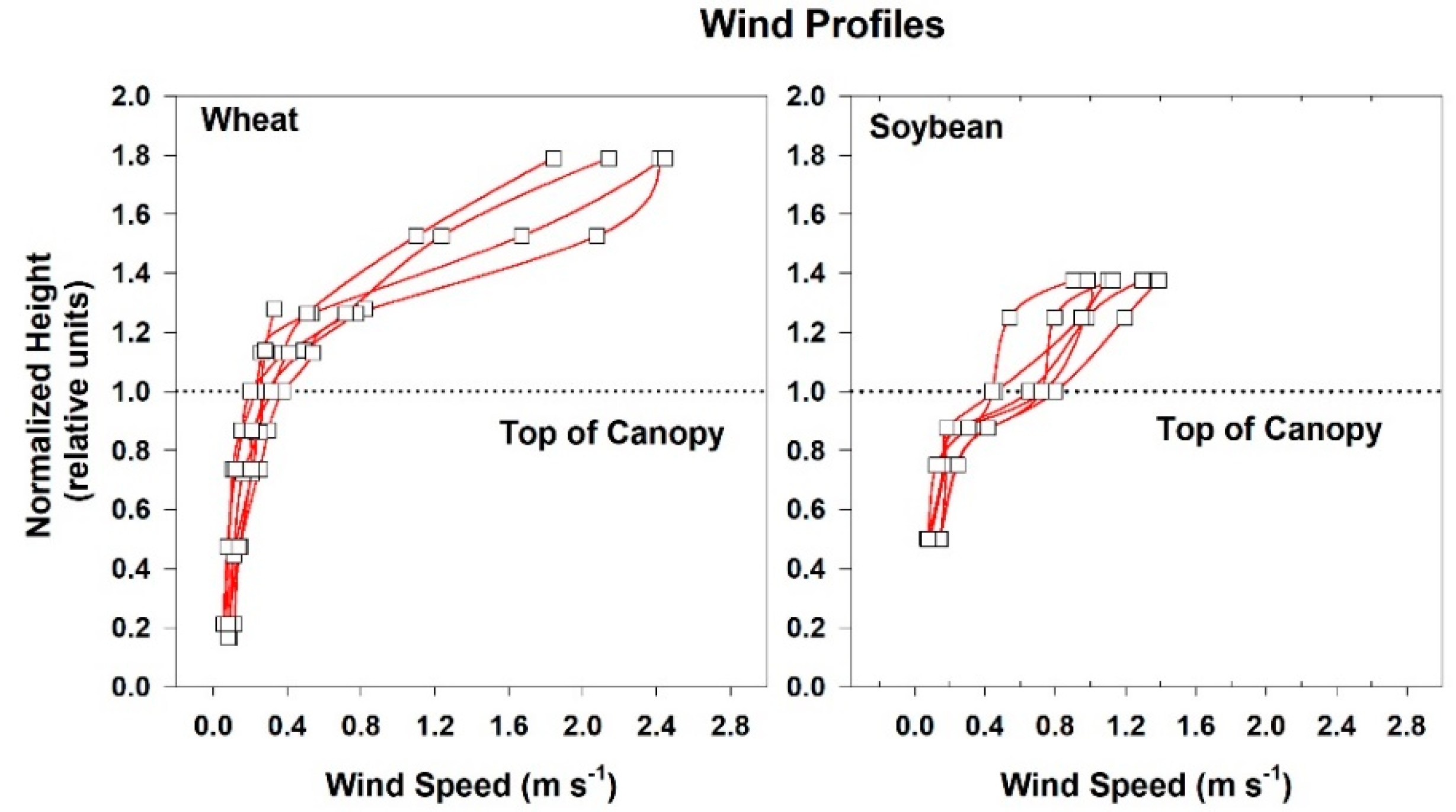
Average wind speed and air temperature profiles were measured at different heights above and within wheat and soybean canopies in a ventilated chamber. The mean wind speed at any given plane above the canopy was highly spatially and temporally variable, typically ranging from 0.5 to 2.4 m s−1 in wheat (Figure 2A), and from 0.4 to 1.4 m s−1 in soybean (Figure 2B). The average wind speed at the canopy surface was attenuated rapidly within the first few centimeters of foliage. Wind speed within the canopies was more uniform than above and was often below 0.4 m s−1, reaching as low as 0.1 m s−1 at the bottom of the wheat canopy.
Vertical air temperature profiles within the growth chamber were homogeneous in an empty, dark chamber since there was no foliage to trap pockets of air, and because the surfaces within the chamber (glass and chamber walls, and the surface of the growth media) equilibrated at nearly the same temperature. When the lights were turned on, the vertical air temperature profiles within the canopy were spatially variable; air near the plants could be 1–5 °C higher than the reference air temperature measured above them depending on the relative magnitudes of incident radiation or wind speed within the chamber (Figure 3). These large air temperature differences within the canopies result from vertical differences in light intensity, leaf temperature, and leaf transpiration rates. Transpiration cools cooled the lower layers of the canopy to temperatures below the reference air temperature, and the uppermost leaf layers remain warmer because they are heated by the absorption of incident radiation.
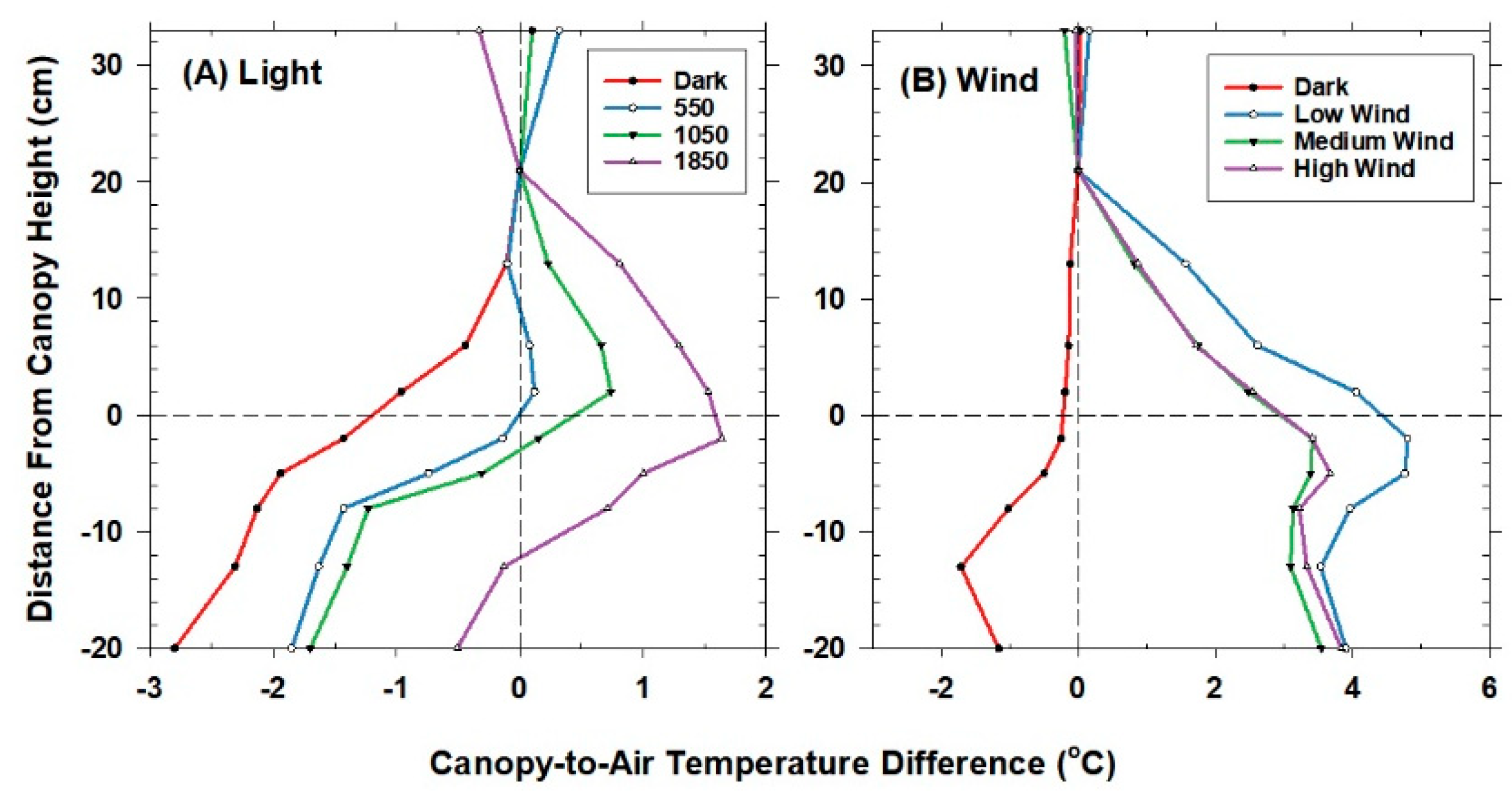
Incident PPF affected the air temperature difference above and within a wheat canopy (Figure 3A; 20-day old; [CO2] = 400 μmol mol−1; Tair = 21 °C; RH = 68%; medium wind speed: 1.7 m s−1). In the dark, the top layers of foliage remained warmer than the lower layers because they were heated by sensible heat flux from the warm chamber air flowing above the canopy. During the photoperiod, the top of the canopy remained hotter than the lower leaf layers as the top layers of foliage absorbed most of the incident radiation. The air within the top 5 cm of the canopy became hotter than the reference air temperature as incident light levels increased to 1050 and 1850 μmol m−2 s−1 (Figure 3A).
At constant PPFo, the fan speed setting (high: 2.3 m s−1; medium: 1.7 m s−1; low: 0.8 m s−1) changed the amount of forced convection in the chamber and affected the vertical air temperature profiles above and within the wheat canopy (Figure 3B; 35-day old; PPF = 1800 μmol m−2 s−1; [CO2] = 1200 μmol mol−1; Tair = 21 °C; RH = 68%). At the low chamber wind speed setting (0.8 m s−1), the upper 7 cm of the canopy was 1.5 °C warmer than at medium (1.7 m s−1) and high (2.3 m s−1) settings (Figure 3B). Air temperature up to 12 cm above the canopy was also heated by 0.5–1.2 °C by the warm foliage at the low wind speed. This suggests a threshold in turbulence in the chamber, above which an increase in wind speed does not continue to affect canopy-air heat exchange.
3.2. Diurnal Changes in Energy Balance Components
Sensible heat flux (Figure 4; pink line) was calculated from direct measurements of canopy energy balance components (net radiation—red line; latent heat—blue line; photosynthesis—green line) in wheat (18-day-old; [CO2] = 680 μmol mol−1; PPF = 1600 μmol m−2 s−1; Tair = 21 °C; RH = 68%) and soybean (25-day-old; [CO2] = 1200 μmol mol−1; PPF = 750 μmol m−2 s−1; Tair = 21 °C; RH = 64%) using Equation (5). In the dark, net radiation was negligible and the canopies were always cooler than air temperature because the transpiration rate and latent heat flux of hydroponic plants remains high [42]. However, the topmost leaf layers remained warm compared to the lower layers of the canopy (Figure 3A), as advection of warm air from the chamber temperature control system supplies additional energy for transpiration. Latent heat increased and sensible heat decreased in the hours preceding the photoperiod (Figure 4), probably due to circadian increases in predawn stomatal conductance [43].
Generally, sensible heat increased during the photoperiod as the canopy became warmer because evaporative cooling from latent heat diminished during the course of the day, even though incident PPF was constant. This decrease in latent heat is probably due to diurnal changes in stomatal conductance [42]. In wheat, sensible heat was negative whenever latent heat plus photosynthesis exceeded net radiation, but the canopy became hotter than air temperature and sensible heat was positive at the end of the day (Figure 4A). The soybean canopy remained cooler than the air temperature, and latent heat remained greater than net radiation in spite of decreasing latent heat at the end of the day (Figure 4B).
3.3. Canopy-to-Air Teperature Difference
The difference between aerodynamic ΔTA and radiometric ΔTIR is affected by two physical factors: the field of view of the IR transducers and the chamber wind speed. The field of view of the sensor with respect to the canopy surface influenced the magnitude of the radiometric TR measured by the infrared transducers. Differences in TIR and TAero are probably due to differences in how well radiometric measurements truly represent the average canopy temperature profile. With constant Tair and PPFo provided by the chamber, radiometric TR was affected by the vertical positioning of the infrared transducers above or within the canopy. Generally, TR was higher in the surface layers of foliage and became lower as the IR transducer was inserted into the canopy foliage. Once the IR transducers were positioned, the canopy-to-air temperature difference was compared to the canopy-to-air temperature difference obtained from H.
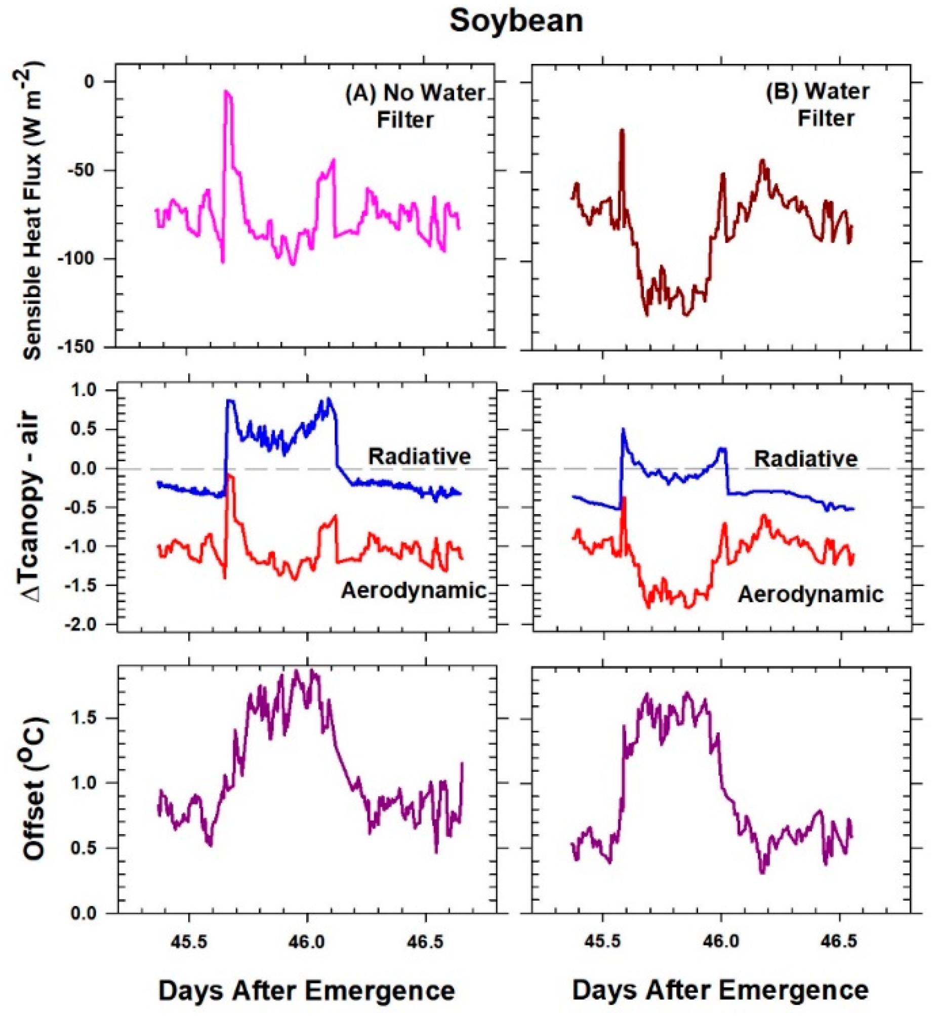
The relation between H, ΔTIR, and ΔTA was explored in soybean by changing the amount and quality of incident radiation (Figure 5; 45-day-old; [CO2] = 400 μmol mol−1; PPF = 1050 μmol m−2 s−1; Tair = 22 °C; RH = 62%). In the dark, the energy balance components under each water filter were similar, yielding H ~ −75 W m−2 (Figure 5, top), but radiometric ΔTIR and aerodynamic ΔTA differed by a nearly constant offset (Figure 5, bottom). The spikes in H observed at the beginning and at the end of the photoperiod are artifacts that occur when H is obtained by subtraction and chamber energy fluxes and temperatures equilibrate.
During the photoperiod, removing the water filter under the HPS lamps increased Rnet by ~50 W m−2 due to a 30% greater PPFo transmission and due to increased longwave radiation as the lamps heated the glass of the water filter. Without the water filter, the ratio of photosynthetic to non-photosynthetic shortwave radiation dropped from 83:17 to 66:34, and sensible heat flux increased up to approximately −95 W m−2 (Figure 5A, top), from approximately −120 W m−2 (Figure 5B, top) as the additional radiation from the lamps warmed the canopy. Radiometric ΔTIR was consistently higher than aerodynamic ΔTA, and the offset was between 0.8 and 1.0 °C higher than it was in the dark. In fact, the sensible heat flux calculated from ΔTIR using Equation (6) often had an opposite sign to values of sensible heat flux calculated from the energy balance equation (Figure 5, middle).
However, relative changes in the magnitude of ΔTIR as a function of time paralleled the relative changes in H and ΔTA (Figure 5, bottom), and the difference between the measured ΔTIR and ΔTA remained constant throughout the photoperiod.
Wind speed determines canopy gA and affects how the foliage warms as PPFo is increased. In a wheat canopy (25-day-old; [CO2] = 1200 μmol mol−1; Tair = 22 °C; RH = 68%; no water filter), changes in PPFo at two chamber wind speeds were used to explore the offset between ΔTA and ΔTIR (Figure 6). At each wind speed, ΔTA calculated from H by inverting Equation (6) was compared with values of ΔTIR measured by the IR sensors.
As incident PPFo increased from 0 to 1700 µmol m−2 s−1, ΔTIR increased linearly from 0 °C to +4 °C at low wind speed (Figure 6A, top; 1.7 m s−1) and increased from −1 °C to +2 °C at high wind speed (Figure 6B, top; 2.3 m s−1). Although the aerodynamic ΔTA also increased linearly with increasing PPFo (Figure 6A,B), its sign was negative at low to moderate light levels and it had a steeper response to PPFo than ΔTIR (e.g., changing from −3 °C to +4 °C at the low wind setting; Figure 6A).
The radiometric ΔTIR never equaled zero when ΔTA was zero (Figure 6) and was often opposite in sign to the aerodynamic ΔTA (Figure 6A,B, top). The offset correction between the radiometric ΔTIR and the aerodynamic ΔTA increased linearly with increasing PPFo, but did not vary with chamber wind speed (Figure 6A,B, bottom graphs; the dashed lines are the 95% confidence interval). Smaller values of the offset at high light intensities suggest that the warmer leaves at the top of the canopy play a greater role in H and reduce the differences between TR and TAero.
This analysis suggests that ΔTIR cannot be used to determine H directly, that is, without correcting for the offset. Thus, the offset in part corrects estimates of H for differences between ΔTIR and ΔTA and allows Equations (6) and (7) to accurately describe the energy balance of dense canopies.
3.4. Canopy Aerodynamic Conductance
In controlled-environment chambers, gA is determined by an interaction between canopy architecture and air circulation in the chamber. Typically, fan speed is constant and canopy architecture remains constant over several days once the canopy is closed. In these conditions, Equation (6) permits canopy gA to be calculated from the slope of a plot of H versus ΔTIR. Stepwise increases in chamber CO2 concentration from 400 to 1200 μmol mol−1 were used to simultaneously alter H and ΔTIR via physiological changes in canopy GS at a constant canopy gA. H and ΔTIR increase simultaneously when chamber ambient CO2 increases because elevated CO2 reduces stomatal conductance, and the canopy is warmed due to less evaporative cooling.
A plot of H and radiometric ΔTIR was used to calculate the gA of a wheat canopy (Figure 7; 25-day-old; PPF = 1200 μmol m−2 s−1; Tair = 22 °C; RH = 70%). The slopes of H versus ΔTIR at each CO2 concentration were similar (separate regressions not shown in Figure 7), which suggests that gA did not respond to changes in ambient CO2.
The variability in H (~±25 W m−2) corresponds to an uncertainty in ΔTIR of ~±0.4 °C, which is close to the error in determining TR from Tcanopy,IR. The dashed line in Figure 7 represents the plot of H versus ΔTA, determined by subtracting a constant offset to ΔTIR (Equation (7)). This offset equals the value of the difference between ΔTIR and ΔTA when H is zero. In wheat, this offset was +0.75 °C at 1600 μmol m−2 s−1 and was +1.0 °C in soybean at 750 μmol m−2 s−1.
The gA of the 25-day-old wheat canopy was 5.5 mol m−2 s−1 (Figure 7). The gA of a 45-day-old soybean canopy was 2.5 mol m−2 s−1. These conductances correspond to aerodynamic resistances of 7.5 and 16.5 s m−1, respectively. Soybean has a smaller gA compared to wheat because soybean leaves are wider than wheat leaves and have a smaller leaf boundary layer conductance.
3.5. Canopy Surface and Stomatal Conductances
Canopy surface GSFC of wheat was calculated from Ecan and DS using Equation (8) (green line; Figure 8A; 26-day-old; [CO2] = 400 μmol mol−1; PPF = 1600 μmol m−2 s−1; Tair = 21 °C; RH = 68%). Once gA was determined, GSFC was used for estimating canopy GS using Equation (9) (green line; Figure 8B). Assuming that canopy GS equals GSFC, that is, without taking gA into account (green lines in Figure 8A,B) underestimates GS by 40% in wheat.
The sensitivity of GSFC (Equation (8)) to errors from using ΔTIR instead of ΔTA was also explored (Figure 8). Surface GSFC of wheat (Figure 8A) was only slightly greater when calculated from radiometric TR instead of aerodynamic TAero. The average surface GSFC at the radiometric TR was 1.6 mol m−2 s−1 (red line; Figure 8A) and 1.5 mol m−2 s−1 (green line; Figure 8A) at the aerodynamic TAero. Therefore, neglecting the offset correction between ΔTIR and ΔTA in wheat resulted in only a –6% error in surface GSFC. The difference between the average radiometric GS (2.3 mol m−2 s−1 or 18.0 s m−1) and aerodynamic GS (2.1 mol m−2 s−1 or 19.7 s m−1) was also small (red vs. green line; Figure 8B). Thus, canopy GS of wheat computed using the observed TR instead of TAero was only 8% higher.
In soybean at 400 μmol mol−1 of CO2, the surface radiometric GSFC was 0.56 mol m−2 s−1 and aerodynamic GSFC was 0.75 mol m−2 s−1, thus using TR instead of TAero to estimate surface GSFC of soybean resulted in a larger (−34%) error. The corresponding radiometric and aerodynamic values of canopy GS were 0.7 mol m−2 s−1 and 1.1 mol m−2 s−1, a difference of 49%.
In wheat, the sensitivity of GSFC to errors in gA was examined by comparing the measured GSFC with the GSFC obtained from the observed GS and a typical value of field gA reported in the literature (gA = 2 mol m−2 s−1; [44]). This field value of gA corresponds to less turbulent conditions (a smaller gA) than were observed for wheat in the chamber, and it is closer to the gA of soybean. The GSFC calculated by inverting Equation (9) using measured GS and field gA (Figure 8A; dashed line) underestimates the measured GSFC (Figure 8A; green line) by 33%. This analysis shows that large differences in surface GSFC exist between field settings and controlled-environment chambers and that these occur because of differences in turbulence that can be accounted for only when gA is known.
The canopy gA and GS for wheat (18-day-old; [CO2] = 400 μmol mol−1; PPF = 1600 μmol m−2 s−1; Tair = 21 °C; RH = 68%) and soybean (25-day-old; [CO2] = 400 μmol mol−1; PPF = 750 μmol m−2 s−1; Tair = 21 °C; RH = 64%) canopies are reported in Table 2.
3.6. Diurnal Changes in GS
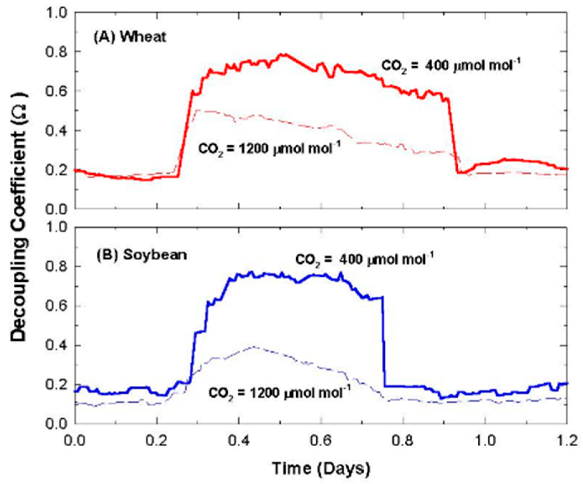
Diurnal changes in Ω reflect changes in GS because chamber gA and DBulk are constant (Equation (10)). The effect of CO2 concentration on the diurnal course of GS was examined in wheat (Figure 9A; (18-day-old; PPF = 1600 μmol m−2 s−1; Tair = 21 °C; RH = 68%)) and soybean (Figure 9B; (27-day-old; PPF = 750 μmol m−2 s−1; Tair = 21 °C; RH = 64%)) canopies.
In the dark, Ω of both canopies was below 0.2, Ds was coupled to DBulk, and canopy transpiration was small. Indeed, the nighttime VPDs within the wheat canopy (DAero 1.12 kPa, and DS 1.15 kPa) were near the VPD (DBulk 1.27 kPa) of the chamber. When the lights came on, the stomata opened, the chamber humidity and Gs increased, the boundary layer within the canopy became humidified by transpiration, and DBulk decreased during the photoperiod. In wheat, VPDs within the canopy (DAero 0.57 kPa and DS 0.36 kPa) became decoupled from DBulk (0.74 kPa). At 400 µmol mol−1 CO2, the mean daily Ω of wheat was 0.67 and 0.55 in soybean (Equation (10); Figure 9) due to the differences in their corresponding GS and gA. Ω during the early part of the day rose to ~0.8 in wheat and to ~0.75 in soybean. As the photoperiod progressed, Ω gradually declined to ~0.6 in wheat and to ~0.6 in soybean as a consequence of a diurnal decrease in GS. At 1200 µmol mol−1 CO2, Ω of wheat and soybean reached a maximum of 0.4 due to reduced stomatal conductance and declined to near 0.2 at the end of the photoperiod (Figure 9).
3.7. Control of Canopy Transpiration by CO2 Concentration
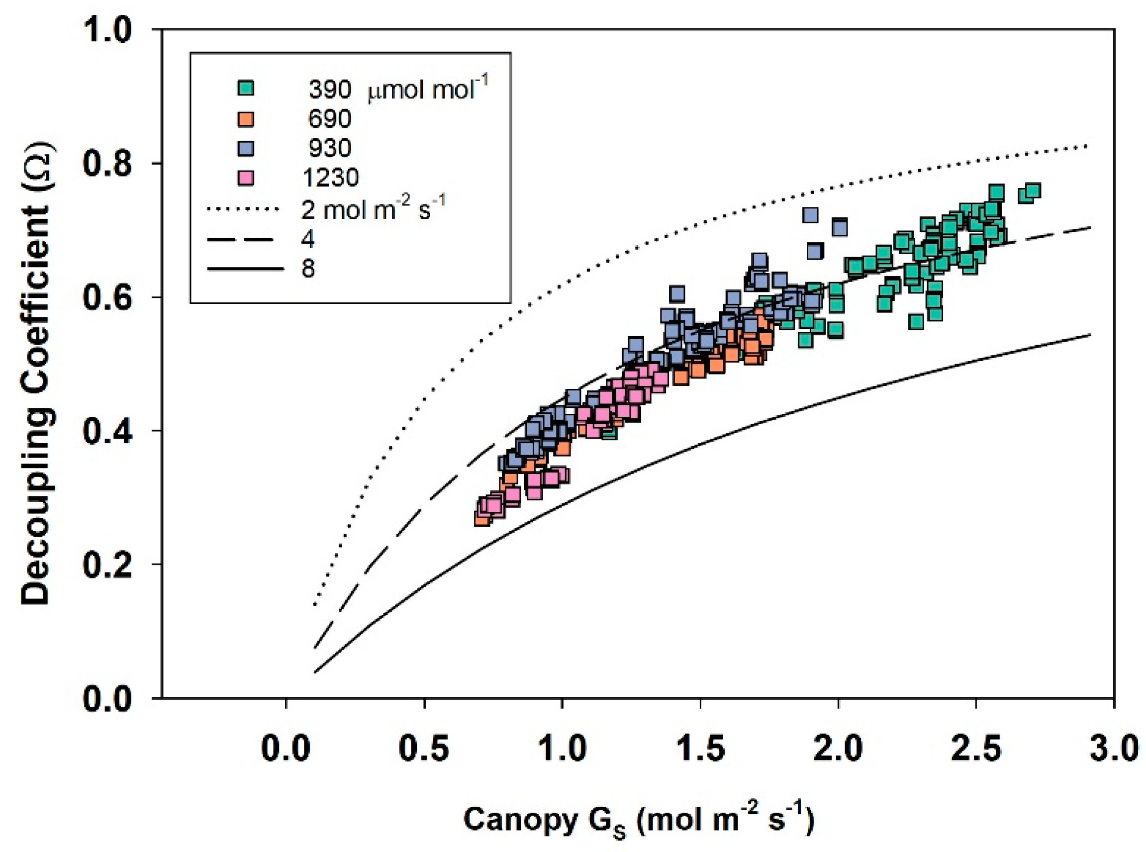
The effect of CO2 concentration on canopy transpiration and Ω was explored using a wheat canopy (27 to 34 day old; PPF = 1600 μmol m−2 s−1; Tair = 21 °C; RH = 68%) exposed to varying chamber CO2 concentrations ranging between 400 and 1200 μmol mol−1 (Figure 10; Table 3).
The CO2 concentration was raised in steps from 400, to 700, to 950, and to 1200 μmol mol−1 and allowing a 48 h acclimation period at each CO2 concentration. Simulated decoupling coefficients were calculated for increasing values of gA (Figure 10; 2 mol m−2 s−1 (dotted line), 4 mol m−2 s−1 (dashed line), and 8 mol m−2 s−1 (solid line)). The decoupling coefficient increased as canopy GS increased, reaching an average Ω of 0.65 with a canopy GS of 2.1 mol m−2 s−1 at 400 μmol mol−1 CO2 (Figure 10; Table 3). Increasing CO2 concentration from 390 to 690 μmol mol−1 led to 1.77 X CO2 or nearly a doubling in ambient CO2. This change decreased mean daily GS by −35%, resulting in a −23% lower transpiration rate and a -23% reduction in latent heat (Table 3). Since gA remained constant, this decrease in GS caused a −26% decrease in Ω. These results indicate that Ecan is less sensitive to changes in stomatal conductance due to the decoupling of Ds from DBulk. In addition, an increase in Pnet of 15% and a −23% decrease in Ecan resulted in a 150% increase in WUE (Table 3).
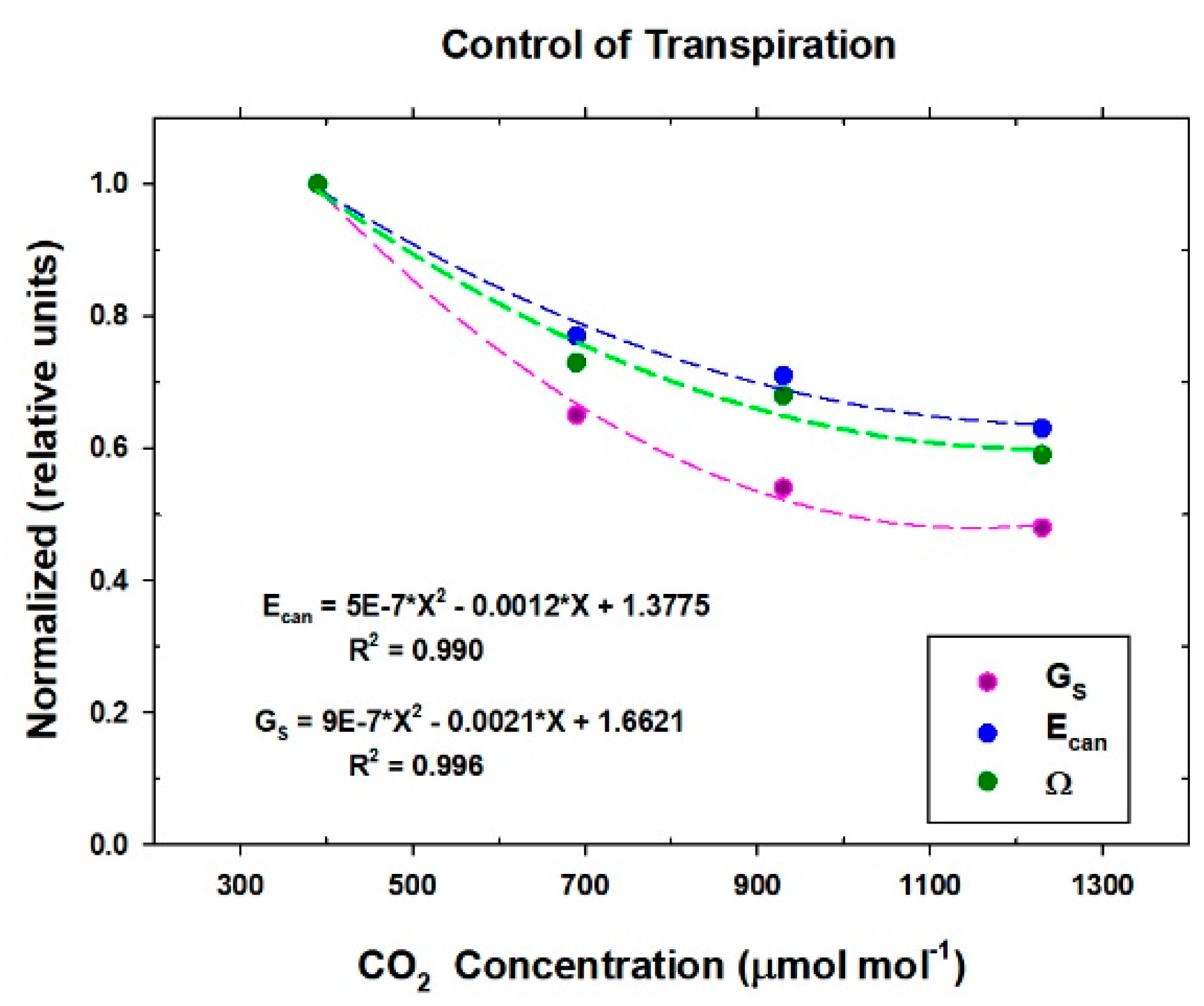
The relative changes in GS, Ecan, and Ω of wheat as CO2 concentration increased, from Table 3, are shown in Figure 11. Canopy GS decreased by 52%, but Ecan only decreased by 37% when CO2 concentration was raised from 390 to 1230 μmol mol−1 because of the feedback between Ecan and DS. In these chamber settings, Ecan is much less sensitive to a proportional change in GS and the reduction in Ecan is largely explained by Ω.
4. Discussion
4.1. Canopy Stomatal Conductance
Land components of climate and carbon models require accurate descriptions of the stomatal control of canopy energy exchange, evapotranspiration, and carbon exchange because land surfaces provide a continuous feedback of latent and sensible heat fluxes to the atmosphere, which drives weather and climate [45]. The method developed in this study expands the usefulness of controlled environments for improving land surface models because it allows the measurement of responses of canopy-level GS, an essential control of canopy gas exchange, to environmental variables.
In this study, GS was measured when surface radiation forcing (Rnet), boundary layer forcing (Tair & DBulk), surface layer feedbacks (gA), and soil moisture were held constant during the photoperiod. Furthermore, the use of well-watered plant stands grown at constant light reduced much of the environmental variability that confounds estimates of GS in natural ecosystems, such as periodic drought, the diurnal change in solar radiation, or short, temporal fluctuations in radiation due to cloud cover. Moreover, the carbon and water vapor fluxes measured in this study do not include significant contributions from soil respiration and evaporation as compared to field measurements.
Canopy GS was derived from direct measurements of surface GSFC, gA, and energy balance (Rnet, LE, and P) in controlled environments. Once the IR transducers were positioned above the canopy, chamber CO2 concentration was manipulated to alter stomatal conductance, which in turn resulted in corresponding changes in sensible heat flux and the canopy–air temperature difference. Canopy gA was obtained radiometrically from the slope of a plot of H vs. ΔTIR (Figure 7), and the offset correcting for differences between TR and Taero was determined.
The radiometric method presented here differs from other methods for calculating GS because canopy gA, Ecan, and canopy-to-air temperature differences are measured directly. This avoids the complexity of methods for scaling leaf level observations to the canopy scale because these must integrate responses of leaf stomatal conductance to vertical profiles in radiation, temperature, humidity, and wind speed within a canopy. Separating gA from the measured canopy GSFC permits the determination of the physiologically controlled canopy-scale GS, which is equivalent to the “big-leaf” stomatal conductance, where the stomatal conductances of individual leaves of the canopy act in parallel, and the vertical gradients in temperature and humidity are averaged by the aerodynamic TAero and DAero. The strength of this approach is that canopy GS responses are measured at the correct scale for predicting ET in future elevated CO2 and climate change scenarios. Furthermore, estimates of canopy ET made using the measured GS also account for the feedback of Ds on ET, as shown by the decoupling coefficient.
In the chamber, gA was set constant by the air flow rate provided by its recirculation fans. However, the gA established in the chamber was different for each species when measured at the same turbulent field provided by the chamber fans. The gA for the wheat (5.5 mol m−2 s−1 or 7.5 s m−1) and for the soybean (2.5 mol m−2 s−1 or 16.5 s m−1) canopies were within the range of typical aerodynamic conductances of field crops (ranging from 3.2–10 mol m−2 s−1 or 4–13 s m−1; [46]). A smaller gA for soybean compared to wheat reflects a larger canopy boundary layer associated with the broader soybean leaves.
In this study, GS values of wheat and soybean were measured at an elevation of 1460 m (4800 ft), a barometric pressure of 86 kPa, and 400 µmol mol−1 CO2 (Table 2). For wheat, GS was 2.3 mol m−2 s−1 or 18 s m−1, which is slightly higher than field GS values (1.8 mol m−2 s−1 or 22.7 s m−1) reported by Hatfield [47] at sea level, under optimal available soil water. The GS of soybean was also slightly higher than typical conductances measured in field crops [46]. Soybean GS at 400 µmol mol−1 CO2 was 1.1 mol m−2 s−1 or 37 s m−1, nearly one-half the value found in wheat probably due to less leaf area and because it was measured at a lower PPFo. The GS values of this study are expected to be higher than those measured at sea level because, at lower atmospheric pressures, the diffusion coefficients of water vapor and CO2 in air increase, so GS also increases [48,49].
4.2. The Control of Transpiration by CO2 Concentration
The radiometric method developed in this study was used to determine the response curve of GS to CO2 concentration in wheat (Figure 11, Table 3). As CO2 concentration increased, the measured decrease in Ecan was lower than the measured decrease in GS because feedback between Ecan and DS operating at the canopy scale effectively reduces the sensitivity of Ecan to changes in GS. Thus, a smaller change in Ecan was observed as CO2 increased, and the reduction in Ecan is largely explained by changes in Ω, which are determined by the relative magnitudes of gA and GS.
In this study, an increase of 1.77 X CO2 (that is, an increase from 390 to 690 μmol mol−1; Table 3) caused a −23% drop in Ecan and a +15% increase in photosynthesis. These changes are comparable to the results of Friend and Cox [50], who used a combined climate-vegetation model to predict a similar −25% drop in ET and a +19.4% increase in GPP for a doubling ambient CO2 (2 X CO2). In a four-year SoyFACE study, Bernacchi et al. [51] found a 9–16% reduction in canopy ET and reported that meta-analyses across FACE experiments indicate a 17–22% drop in leaf level stomatal conductance when daytime CO2 was raised by 175 umol mol−1 from 375 to 550 umol mol−1. In this study, the two regression equations in Figure 11 (Ecan and GS as a function of CO2 concentration) predict a 13% decrease in Ecan and a 22% decrease in canopy GS for an increase of 175 umol mol−1 of CO2. These comparisons suggest that the responses of GS and Ecan to CO2 reported in this study are similar to responses in canopy GS and ET observed in CO2-enriched plant canopies in field settings.
5. Conclusions
The controlled-environment experiments conducted in this study provide a new methodology for measuring canopy stomatal and aerodynamic conductances. A radiometric method for determining canopy aerodynamic conductance from changes in vegetation temperature and energy balance was developed in controlled environments using a canopy-level gas exchange system. The gas exchange system measured canopy gas fluxes (CO2 and water vapor), energy balance (net radiation, latent and sensible heat fluxes), and canopy temperatures as CO2 concentration was varied. Two key assumptions of this method are that radiative canopy temperature is approximated by canopy brightness temperature and that the difference between aerodynamic and radiative canopy-to-air temperature differences is constant during the photoperiod. Once canopy aerodynamic conductance was determined from a plot of sensible heat flux versus the radiative canopy-to-air temperature difference, canopy stomatal conductance was calculated from measurements of canopy transpiration. The method was used to determine the curves of the response of canopy stomatal conductance and canopy ET to increased CO2 concentration in wheat (Table 3; Figure 11). Predictions of canopy ET made from the measured response of GS to elevated CO2 are comparable to land surface model predictions and to observed changes in ET found in FACE studies [50,51]. Future work should focus on studying how canopy stomatal conductance measured using this methodology responds to drought, vapor pressure deficit, and temperature to provide data sets for calibrating global climate models. The method should also be used to characterize how canopy aerodynamic conductance changes during the growth cycle of different crop species.
Author Contributions
O.M. and B.B. conceived the study. O.M. wrote the original manuscript. O.M. and B.B. reviewed and revised the manuscript. Project administration and funding acquisition: B.B. All authors read and approved the manuscript.
Funding
This research was supported by the Advanced Life Support Program of the National Aeronautics and Space Administration and by the Utah State Agricultural Experiment Station, Utah State University. This manuscript has been approved as journal paper number 9178.
Acknowledgments
The authors would like to thank John Norman, Marc Van Iersel, and Larry Hipps for critically reviewing the manuscript.
Conflicts of Interest
The authors declare no conflict of interest. The funders had no role in the design of the study; in the collection, analyses, or interpretation of data; in the writing of the manuscript; or in the decision to publish the results.
Abbreviations
| Symbol | Description | Units |
| Cp | Heat capacity of air at constant pressure | kJ m−3 °C−1 |
| [CO2] | CO2 concentration | umol mol−1 |
| DAE | Days after emergence | d |
| E | Chamber evaporation rate | mmol m−2 s−1 |
| Ecan | Canopy transpiration rate | mmol m−2 s−1 |
| ET = ΔXh20*MF | Chamber evapotranspiration | mmol m−2 s−1 |
| gS | Single leaf stomatal conductance | mol m−2 s−1 |
| gA | Canopy aerodynamic conductance | mol m−2 s−1 |
| G | Soil heat flux | W m−2 |
| GSFC | Canopy surface conductance | mol m−2 s−1 |
| GS | Canopy stomatal conductance | mol m−2 s−1 |
| H | Sensible heat flux | W m−2 |
| LE | Latent heat flux | W m−2 |
| ↑Lc | Longwave radiation emitted by the canopy | W m−2 |
| ↓Lg | Longwave radiation emitted by the glass of the water filter | W m−2 |
| MF | Mass flow rate of air | mol s−1 |
| NPSWabs | Absorbed non-photosynthetic shortwave radiation | W m−2 |
| Offset | Difference between ΔTA and ΔTIR | °C |
| P | Energy storage in photosynthesis | W m−2 |
| Pnet | Canopy net photosynthetic rate | μmol m−2 s−1 |
| PPFo | Incident photosynthetic photon flux | μmol m−2 s−1 |
| PPFabs | Fraction of incident PPF absorbed by the canopy | μmol m−2 s−1 |
| Rnet | Net radiation | W m−2 |
| s | Slope of the relation between saturation vapor pressure and temperature | |
| Tair | Mean air temperature measured above the canopy | °C |
| TAero | Canopy aerodynamic temperature | °C |
| Tcanopy,IR | Canopy brightness temperature measured by IR transducers | °C |
| Tglass, Twall | Water filter glass and chamber wall temperatures | °C |
| TR | Canopy radiometric temperature | °C |
| TSky | Composed of 20% chamber Twall and 80% Tglass | °C |
| γ | Psychrometric constant | kPa K−1 |
| ΔTA | Aerodynamic canopy-to-air temperature difference (TAero − Tair) | °C |
| ΔTIR | Radiometric canopy-to-air temperature difference (TR − Tair) | °C |
| ΔXh20 | Mole fraction difference between pre- and post-chamber water vapor | |
| ε = s/γ | ratio of the increase of latent heat content to the increase of sensible heat content of saturated air | |
| εc | Canopy emissivity | |
| ρ | Density of air | kg m−3 |
| ρc | Canopy reflection coefficient | |
| σ | Stefan–Boltzman constant | W m−2 K−4 |
| σS | Scattering coefficient | |
| Ω | Decoupling coefficient | |
| XH2O(Tair) | Mol fraction of water vapor at Tair above the canopy | |
| XH2O(TAero) | Mol fraction of water vapor at TAero |
References
- Friend, A.D.; Kiang, N.Y. Land surface model development for the GISS GCM: Effects of improved canopy physiology on simulated climate. J. Clim. 2005, 18, 2883–2902. [Google Scholar] [CrossRef]
- Van Heerwaarden, C.C.; Vila-Gerau de Arrellano, J.; Gonou, A.; Guichard, F.; Couvreux, F. Understanding the daily cycle of evapotranspiration: A method to quantify the influence of forcings and feedbacks. J. Hydromet. 2010, 11, 1405–1422. [Google Scholar] [CrossRef]
- Jarvis, P.G.; McNaughton, K.G. Stomatal control of transpiration: Scaling up from leaf to region. Adv. Ecol. Res. 1986, 15, 1–49. [Google Scholar]
- McNaughton, K.G.; Jarvis, P.G. Effects of spatial scale on stomatal control of transpiration. Agric. For. Meteorol. 1991, 54, 279–301. [Google Scholar] [CrossRef]
- Agam, N.; Kustas, W.P.; Anderson, M.C.; Norman, J.M.; Colaizzi, P.D.; Howell, T.A.; Prueger, J.H.; Meyers, T.P.; Wilson, T.B. Application of the Priestley-Taylor approach in a two-source surface energy balance model. J. Hydromet. 2010, 11, 185–198. [Google Scholar] [CrossRef]
- Meinzer, F.C. Stomatal control of transpiration. Trends Ecol. Evol. 1993, 8, 289–294. [Google Scholar] [CrossRef]
- Meinzer, F.C.; Goldstein, G.; Holbrook, N.M.; Jackson, P.; Cavelier, J. Stomatal and environmental control of transpiration in a lowland tropical forest tree. Plant Cell Environ. 1993, 16, 429–436. [Google Scholar] [CrossRef]
- Monteith, J.L.; Unsworth, M.H. Principles of Environmental Physics, 1st ed.; Chapman and Hall, Inc.: New York, USA, 1990; ISBN 9780123869104. [Google Scholar]
- Grace, J.; Wilson, J. The boundary layer over a Populus leaf. J. Exp. Bot. 1976, 27, 231–241. [Google Scholar] [CrossRef]
- Jones, H.G. Plants and Microclimate: A Quantitative Approach to Environmental Plant Physiology; Cambridge University Press: New York, NY, USA, 1992; ISBN 9780521425247. [Google Scholar]
- Brenner, A.J.; Jarvis, P.G. A heated replica technique for determination of leaf boundary layer conductance in the field. Agric. For. Meteorol. 1995, 72, 261–275. [Google Scholar] [CrossRef]
- Bunce, J.A. Use of a minimally invasive method of measuring leaf stomatal conductance to examine stomatal responses to water vapor pressure difference under field conditions. Agric. For. Meteorol. 2006, 139, 335–343. [Google Scholar] [CrossRef]
- Baldocchi, D.D.; Luxmoore, R.J.; Hatfield, J.L. Discerning the forest from the trees: An essay on scaling canopy stomatal conductance. Agric. For. Meteorol. 1991, 54, 197–226. [Google Scholar] [CrossRef]
- Kelliher, F.M.; Leuning, R.; Raupach, M.R.; Schulze, E.D. Maximum conductances for evaporation from global vegetation types. Agric. For. Meteorol. 1995, 73, 1–16. [Google Scholar] [CrossRef]
- Wullschleger, S.D.; Gunderson, C.A.; Hanson, P.J.; Wilson, K.B.; Norby, R.J. Sensitivity of stomatal and canopy conductance to elevated CO2 concentration—interacting variables and perspectives of scale. New Phytol. 2002, 153, 485–496. [Google Scholar] [CrossRef]
- Smith, R.C.G.; Barrs, H.D.; Meyer, W.S. Evaporation from irrigated wheat estimated using radiative surface temperature: an operational approach. Agric. For. Meteorol. 1989, 48, 331–344. [Google Scholar] [CrossRef]
- Choudhury, B.J.; Monteith, J.L. A four-layer model for the heat budget of homogenous land surfaces. Q. J. R. Metereol. Soc. 1988, 114, 373–398. [Google Scholar] [CrossRef]
- Chehbouni, A.; LoSeen, D.; Njoku, E.G.; Monteny, B.M. Examination of the difference between radiative and aerodynamic surface temperatures over sparsely vegetated surfaces. Remote Sens. Environ. 1996, 58, 177–186. [Google Scholar] [CrossRef]
- Campbell, G.S.; Norman, J.M. An introduction to Environmental Biophysics, 1st ed.; Springer: New York, NY, USA, 1998; ISBN 978-1-4612-1626-1. [Google Scholar]
- Crow, W.T.; Kustas, W.P. Utility of assimilating surface radiometric temperature observations for evaporative fraction and heat transfer coefficient retrieval. Boundary-Layer Meteorol. 2005, 115, 105–130. [Google Scholar] [CrossRef]
- Kustas, W.P.; Anderson, M.C.; Norman, J.M.; Li, F. Utility of radiometric-aerodynamic temperature relations for heat flux estimation. Boundary-Layer Meteorol. 2007, 122, 167–187. [Google Scholar] [CrossRef]
- Kimes, D.S. Remote sensing of row crop structure and component temperatures using directional radiometric temperatures and inversion techniques. Remote Sens. Environ. 1983, 13, 33–55. [Google Scholar] [CrossRef]
- Merlin, O.; Chehbouni, A. Different approaches in estimating heat flux using dual angle observations of radiative surface temperature. Int. J. Remote Sens. 2004, 25, 275–289. [Google Scholar] [CrossRef]
- Mahrt, L.; Vickers, D. Bulk formulation of the surface heat flux. Boundary-Layer Meteorol. 2004, 110, 357–379. [Google Scholar] [CrossRef]
- Matsushima, D. Relations between aerodynamic parameters of heat transfer and thermal infrared thermometry in the bulk surface formulation. J. Meteorol. Soc. Jpn 2005, 83, 373–389. [Google Scholar] [CrossRef]
- Huband, N.D.S.; Monteith, J.L. Radiative surface temperature and energy balance of a wheat canopy. I. Comparison of radiative and aerodynamic temperature. Boundary-Layer Meteorol. 1986, 36, 1–17. [Google Scholar] [CrossRef]
- Kustas, W.P.; Norman, J.M. A two-source energy balance approach using directional radiometric temperature observations for sparse canopy covered surfaces. Agron. J. 2000, 92, 847–854. [Google Scholar] [CrossRef]
- Norman, J.M.; Becker, F. Terminology in thermal infrared remote sensing of natural surfaces. Remote Sens. Rev. 1995, 12, 159–173. [Google Scholar] [CrossRef]
- Bugbee, B.; Droter, M.; Monje, O.; Tanner, B. Evaluation and modification of commercial infrared transducers for leaf temperature measurement. Adv. Space Res. 1997, 22, 1425–1434. [Google Scholar] [CrossRef]
- Monje, O.; Bugbee, B. Adaptation of plant communities to elevated CO2: radiation capture, canopy quantum yield, and carbon use efficiency. Plant Cell Environ. 1998, 21, 315–324. [Google Scholar] [CrossRef]
- Bugbee, B. Steady state gas exchange in growth chambers: system design and operation. HortScience 1992, 27, 770–776. [Google Scholar] [CrossRef] [PubMed]
- Pearcy, R.W.; Schulze, E.D.; Zimmermann, R. Measurement of transpiration and leaf conductance. In Plant Physiological Ecology: Field Methods and Instrumentation; Pearcy, R.W., Ehleringer, R.W., Mooney, J.R., Rundel, P.W., Eds.; Springer: Dordrecht, The Netherlands, Chapter 8; pp. 137–160. ISBN 978-94-010-9013-1.
- Bugbee, B.; Monje, O.; Tanner, B. Quantifying energy and mass transfer in crop canopies. Adv. Space Res. 1996, 18, 149–156. [Google Scholar] [CrossRef]
- Ross, J. The Radiation Regime and Architecture of Plant Stands; Dr W. Junk Publishers: The Hague, The Netherlands, 1981; ISBN 978-94-009-8647-3. [Google Scholar]
- Goudriaan, J.; van Laar, H.H. Modeling Potential Crop Growth Processes: Textbook with Exercises, 1st ed.; Kluwer Academic Publishers: Boston, MA, USA, 1994; ISBN 978-94-011-0750-1. [Google Scholar]
- Monje, O. Effects of elevated CO2 on crop growth rates, radiation absorption, canopy quantum yield, canopy carbon use efficiency, and root respiration of wheat. M.S. Thesis, Utah State University, Logan, UT, USA, 1993. [Google Scholar]
- Liang, S.; Strahler, A.H.; Jin, X.; Zhut, Q. Comparisons of radiative transfer models of vegetation canopies and laboratory measurements. Remote Sens. Environ. 1997, 61, 129–138. [Google Scholar] [CrossRef]
- Wang, Y.P. A comparison of three different canopy radiation models commonly used in plant modeling. Func. Plant Biol. 2003, 30, 143–152. [Google Scholar] [CrossRef]
- Bubenheim, D.L.; Bugbee, B.; Salisbury, F.B. Radiation in controlled environments: Influence of lamp type and filter material. Am. Soc. Hort. Sci. 1988, 113, 468–474. [Google Scholar]
- Bugbee, B.; Monje, O. The optimization of crop productivity: Theory and validation. Bioscience 1992, 42, 494–502. [Google Scholar] [CrossRef] [PubMed]
- Chehbouni, A.; Nichols, W.D.; Njoku, E.G.; Qi, J.; Kerr, Y.H.; Cabot, F. A three component model to estimate sensible heat flux over sparse shrubs in Nevada. Remote Sens. Rev. 1997, 15, 99–112. [Google Scholar] [CrossRef]
- Monje, O.; Bugbee, B. Characterizing photosynthesis and transpiration of plant communities in controlled environments. Acta Hortic. 1996, 440, 123–128. [Google Scholar] [CrossRef] [PubMed]
- Resco de Dios, V.; Loik, M.E.; Smith, R.; Aspinwall, M.J.; Tissue, D.T. Genetic variation in circadian regulation of nocturnal stomatal conductance enhances carbon assimilation and growth. Plant Cell Environ. 2016, 39, 3–11. [Google Scholar] [CrossRef] [PubMed]
- Luchiari, A.; Riha, S.J. Bulk surface conductance and its effect on evapotranspiration rates in irrigated wheat. Agron. J. 1991, 83, 888–895. [Google Scholar] [CrossRef]
- Dai, J.; Dickinson, R.E.; Wang, Y. A two-big-leaf model for canopy temperature, photosynthesis, and stomatal conductance. J. Clim. 2004, 17, 2281–2299. [Google Scholar] [CrossRef]
- O’Toole, J.C.; Real, J.G. Estimation of aerodynamic and crop resistances from canopy temperature. Agron. J. 1986, 78, 305–310. [Google Scholar] [CrossRef]
- Hatfield, J.L. Wheat canopy resistance determined by energy balance techniques. Agron. J. 1985, 77, 279–283. [Google Scholar] [CrossRef]
- Gale, J. Availability of carbon dioxide for photosynthesis at high altitudes: Theoretical considerations. Ecology 1972, 53, 494–497. [Google Scholar] [CrossRef]
- Daunicht, H.J.; Brinkhans, H.J. Gas exchange and growth of plants under reduced air pressure. Adv. Space Res. 1992, 12, 107–114. [Google Scholar] [CrossRef]
- Friend, A.D.; Cox, P.M. Modelling the effects of atmospheric CO2 on vegetation-atmosphere interactions. Agric. For. Meteorol. 1995, 73, 285–295. [Google Scholar] [CrossRef]
- Bernacchi, C.J.; Kimball, B.A.; Quarles, D.R.; Long, S.P.; Ort, D.R. Decreases in stomatal conductance of soybean under open-air elevation of [CO2] are closely coupled with decreases in ecosystem evapotranspiration. Plant Physiol. 2007, 143, 134–144. [Google Scholar] [CrossRef] [PubMed]
Figure 1.
A two chamber, open gas exchange system capable of determining canopy aerodynamic conductance from measures of sensible heat flux and canopy-to-air temperature difference was used to calculate canopy stomatal conductances of wheat and soybean canopies.
Figure 1.
A two chamber, open gas exchange system capable of determining canopy aerodynamic conductance from measures of sensible heat flux and canopy-to-air temperature difference was used to calculate canopy stomatal conductances of wheat and soybean canopies.
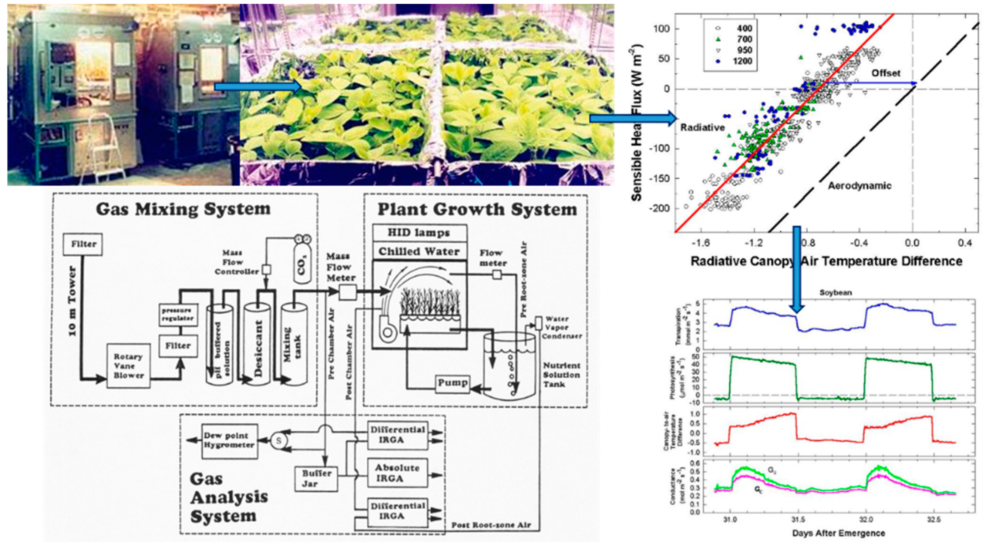
Figure 2.
Vertical wind profiles of wheat and soybean canopies measured with needle anemometers. Y-axis units are fraction of canopy height.
Figure 2.
Vertical wind profiles of wheat and soybean canopies measured with needle anemometers. Y-axis units are fraction of canopy height.

Figure 3.
Vertical canopy-to-air temperature difference profiles of wheat canopies were affected by (A) light intensity and (B) chamber wind speed.
Figure 3.
Vertical canopy-to-air temperature difference profiles of wheat canopies were affected by (A) light intensity and (B) chamber wind speed.

Figure 4.
Diurnal course of canopy energy balance components: net radiation, latent heat flux, sensible heat flux, and photosynthesis in (A) wheat and (B) soybean canopies.
Figure 4.
Diurnal course of canopy energy balance components: net radiation, latent heat flux, sensible heat flux, and photosynthesis in (A) wheat and (B) soybean canopies.
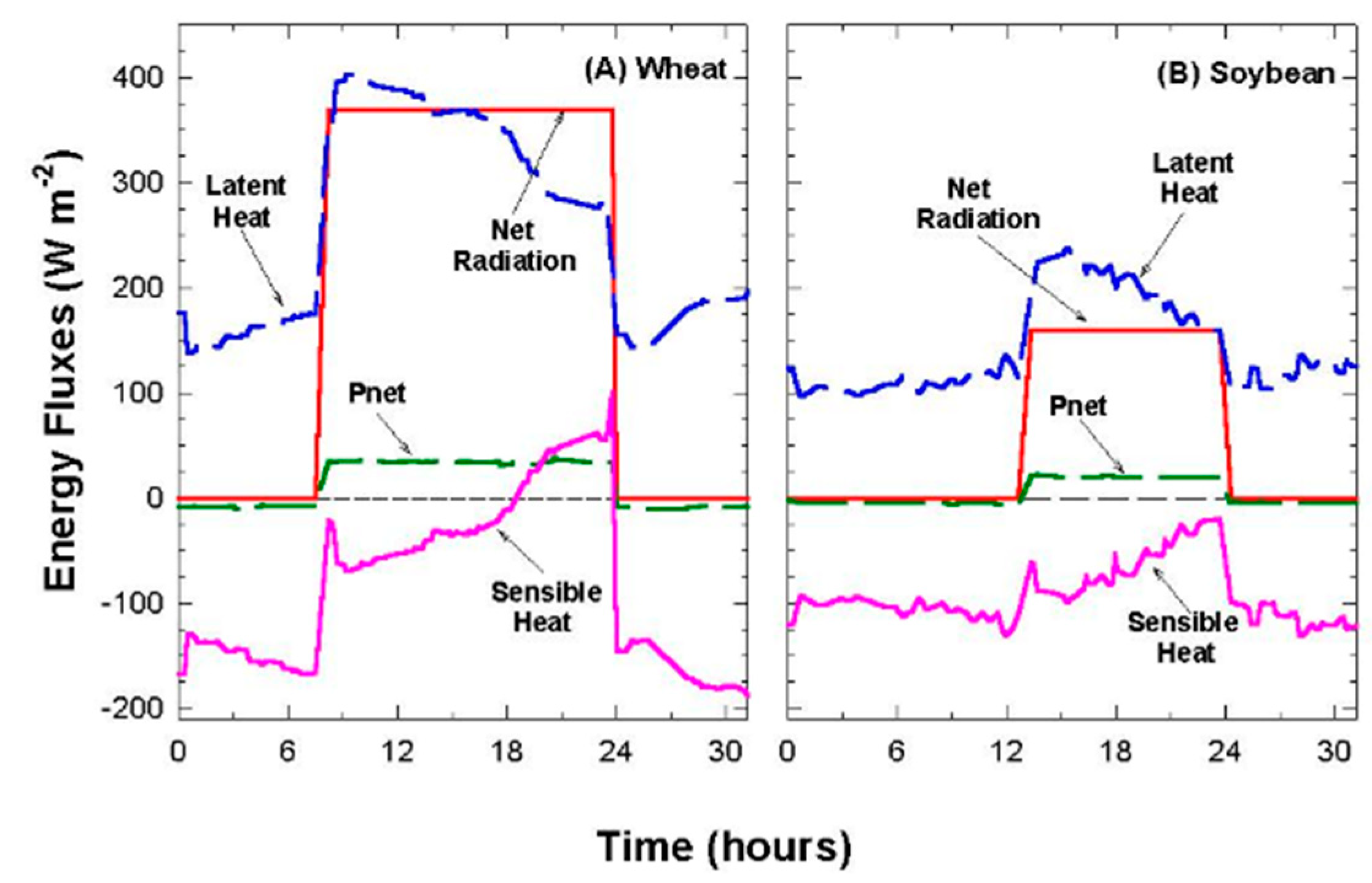
Figure 5.
Diurnal changes in canopy sensible heat, radiative, and aerodynamic canopy-to-air temperature differences, and the offset of soybean illuminated by lamps (A) without and (B) with a water filter to remove excess longwave radiation.
Figure 5.
Diurnal changes in canopy sensible heat, radiative, and aerodynamic canopy-to-air temperature differences, and the offset of soybean illuminated by lamps (A) without and (B) with a water filter to remove excess longwave radiation.

Figure 6.
The radiometric (ΔTIR) and aerodynamic (ΔTA) temperatures and the offset were measured at (A) low and (B) high chamber wind speed settings.
Figure 6.
The radiometric (ΔTIR) and aerodynamic (ΔTA) temperatures and the offset were measured at (A) low and (B) high chamber wind speed settings.
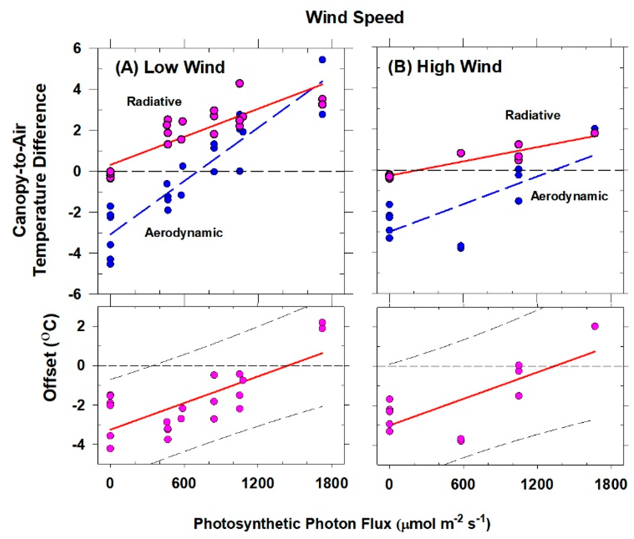
Figure 7.
Plot of H versus ΔTIR (red line) and the offset from a 25-day-old wheat canopy exposed to changing CO2 concentration.
Figure 7.
Plot of H versus ΔTIR (red line) and the offset from a 25-day-old wheat canopy exposed to changing CO2 concentration.
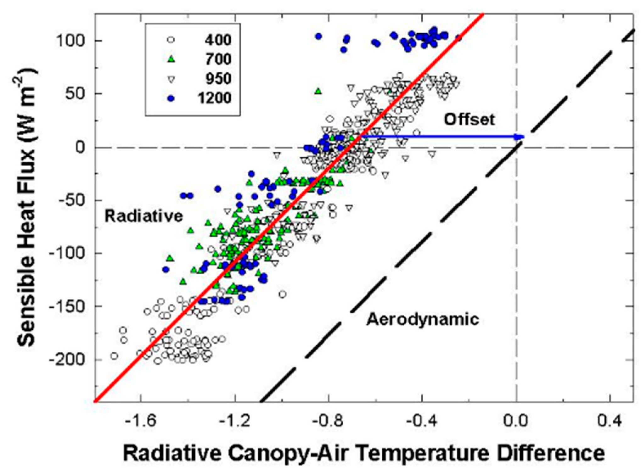
Figure 8.
Daily courses of (A) canopy surface stomatal conductance (GSFC; Equation (8)), and (B) canopy stomatal conductance (GS; Equation (9)) of wheat.
Figure 8.
Daily courses of (A) canopy surface stomatal conductance (GSFC; Equation (8)), and (B) canopy stomatal conductance (GS; Equation (9)) of wheat.
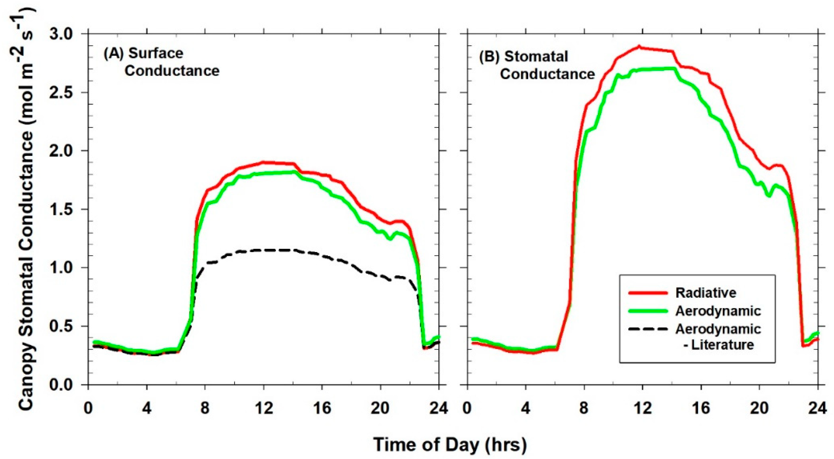
Figure 9.
Diurnal changes in Ω of (A) wheat and (B) soybean at two chamber CO2 concentrations.

Figure 10.
The decoupling coefficient, Ω, expressed as a function of canopy GS in wheat measured at CO2 concentrations ranging between 400 and 1200 μmol mol−1.
Figure 10.
The decoupling coefficient, Ω, expressed as a function of canopy GS in wheat measured at CO2 concentrations ranging between 400 and 1200 μmol mol−1.

Figure 11.
Relative changes in GS, Ecan, and Ω as chamber CO2 concentration increases.

Table 1.
Typical land surface properties that influence the control of transpiration rate from conifers or crops.
Table 1.
Typical land surface properties that influence the control of transpiration rate from conifers or crops.
| Species | Coupling | TAero − Tair | gA | Ω | Relative Magnitude | Transpiration Control |
|---|---|---|---|---|---|---|
| Conifer | coupled | small | low | ~ 0.1 | gA >> GS | Radiation ≈ ΔRnet |
| Crop | decoupled | large | high | ~ 0.8 | gA << GS | Stomatal ≈ ΔGS |
Table 2.
Canopy gA, GS, and Ω from two crop architectures at 400 umol mol−1 CO2 and 86 kPa.
| Species | Architecture | gA 1 | Gs | Ω | Ds-DBulk 2 | DBulk |
|---|---|---|---|---|---|---|
| Wheat | Erectophile | 5.5 (7.5) | 2.3 (18) | 0.67 | 0.38 | 0.74 |
| Soybean | Planophile | 2.5 (16.5) | 1.1 ( 37) | 0.39 | 0.56 | 1.15 |
1 μmol m−2 s−1 (s m−1). 2 kPa.
Table 3.
Canopy level responses to elevated CO2 at constant PPFo and gA.
| CO2 Concentration (µmol mol−1) | ||||||
|---|---|---|---|---|---|---|
| Parameter | Symbol | Units | 390 | 690 | 930 | 1230 |
| Transpiration | Ecan | mmol m−2 s−1 | 11.2 | 8.7 | 7.9 | 7.0 |
| % | 100 | 77 | 71 | 63 | ||
| Photosynthesis | Acan | μmol m−2 s−1 | 63 | 73 | 81 | 79 |
| % | 100 | 115 | 128 | 125 | ||
| Latent Heat | LE | W m−2 | 460 | 356 | 324 | 288 |
| Sensible Heat | H | W m−2 | −175 | −70 | −42 | −3 |
| Stomatal Conductance | GS | mmol m−2 s−1 | 2145 | 1394 | 1152 | 1031 |
| % | 100 | 65 | 54 | 48 | ||
| Decoupling coefficient | Ω | dim. | 0.65 | 0.48 | 0.45 | 0.39 |
| % | 100 | 74 | 69 | 60 | ||
| Water Use Efficiency | WUE | μmol mmol−1 | 5.6 | 8.4 | 10.2 | 11.2 |
| % | 100 | 150 | 183 | 199 | ||
| Changes in Ecan, Gs, LE as CO2 increased from 400 μmol mol−1 | dEcan | mmol m−2 s−1 | - | 2.5 | 3.3 | 4.2 |
| dLE | W m−2 | - | 104 | 136 | 172 | |
| dGS | mol m−2 s−1 | - | 0.75 | 0.99 | 1.11 | |
| dEcan/dGS | mmol mol−1 | - | 3.33 | 3.32 | 3.75 | |
© 2019 by the authors. Licensee MDPI, Basel, Switzerland. This article is an open access article distributed under the terms and conditions of the Creative Commons Attribution (CC BY) license (http://creativecommons.org/licenses/by/4.0/).
Share and Cite
MDPI and ACS Style
Monje, O.; Bugbee, B. Radiometric Method for Determining Canopy Stomatal Conductance in Controlled Environments. Agronomy 2019, 9, 114. https://doi.org/10.3390/agronomy9030114
AMA Style
Monje O, Bugbee B. Radiometric Method for Determining Canopy Stomatal Conductance in Controlled Environments. Agronomy. 2019; 9(3):114. https://doi.org/10.3390/agronomy9030114
Chicago/Turabian StyleMonje, Oscar, and Bruce Bugbee. 2019. "Radiometric Method for Determining Canopy Stomatal Conductance in Controlled Environments" Agronomy 9, no. 3: 114. https://doi.org/10.3390/agronomy9030114
Note that from the first issue of 2016, this journal uses article numbers instead of page numbers. See further details here.