Economic Sustainability of Small-Scale Aquaponic Systems for Food Self-Production
by
 , and
, and
José Lobillo-Eguíbar
1, 
Víctor M. Fernández-Cabanás
1 ,
,
Luis Alberto Bermejo
2 and
and
Luis Pérez-Urrestarazu
3,*
1
Urban Greening and Biosystems Engineering Research Group, Dpto. Ciencias Agroforestales, Universidad de Sevilla, ETSIA, Ctra. Utrera km.1, 41013 Seville, Spain
2
Área de Economía, Sociología y Política Agraria, Escuela Politécnica Superior de Ingeniería, Avenida Ángel Guimerá Jorge s/n, Universidad de La laguna (ULL), 38200 San Cristóbal de La Laguna (Tenerife), Spain
3
Urban Greening and Biosystems Engineering Research Group, Area of Agro-Forestry Engineering, Universidad de Sevilla, ETSIA, Ctra. Utrera km.1, 41013 Seville, Spain
*
Author to whom correspondence should be addressed.
Agronomy 2020, 10(10), 1468; https://doi.org/10.3390/agronomy10101468
Submission received: 20 August 2020
/
Revised: 21 September 2020
/
Accepted: 23 September 2020
/
Published: 25 September 2020
Abstract
:Aquaponics involves the simultaneous production of plants and fish and it is increasingly being used with a self-consumption purpose. However, there are uncertainties and little information about the economic sustainability of small-scale self-managed aquaponic systems. The objective of this study was to obtain economic information about these systems, including the level of commoditization of food production as a measure of their autonomy. For this purpose, two small-scale aquaponic systems (SAS) based on FAO models were self-constructed using cheap and easy-to-obtain materials and monitored for a year. A total of 62 kg of tilapia and 352 kg of 22 different vegetables and fruits were produced, with an average net agricultural added value of 151.3 €. Results showed positive accounting profit but negative economic profit when labor costs were included. The degree of commoditization was around 44%, which allows a certain autonomy, thanks to the use of family labor force.
1. Introduction
Aquaponics is a technique that combines the simultaneous production of plants and fish, and it is often presented as a more sustainable method for food production, given that it aims to optimize the resources employed to grow both vegetables and fish, minimizing pollution (e.g., wastewater) [1]. To do so, the water employed in the aquaculture subsystem is fed to the hydroponic subsystem. The metabolic waste from fish and unconsumed feed is transformed by a bacterial community into easily assimilated nutrients (i.e., nitrates, phosphates) that plants use to grow. After plant nutrient extraction, the water may be returned to the fish tanks (in coupled systems) [2,3,4].
Aquaponic production can have different objectives: commercial [5,6], educational [7], as entertainment or a hobby, research [8] or food production for subsistence and domestic use (familial self-consumption). For this last purpose, low-cost, small-scale aquaponic systems (SAS) [5] have been developed. As one of the main examples, the Food and Agriculture Organization of the United Nations (FAO) proposed in one of its handbooks [9] three small aquaponic units whose main difference was the hydroponic sub-system utilized (media beds, nutrient film technique and deep water culture). Other different types of SAS are proposed [10,11,12], with various degrees of technological development, some of them based on the original FAO designs.
As a distinct characteristic, SAS can be adapted to many locations (rural, peri-urban and urban), but they are particularly interesting in places with reduced space for food production, as happens in urban environments (e.g., vegetable gardens, backyards, buildings’ rooftops) [5,13]. For this reason, domestic/small-scale aquaponic production has proliferated worldwide and, although there are no reliable official census data, the use of this type of aquaponics system is a growing trend [14], especially in urban settlements [15].
However, the economic sustainability of aquaponic systems is not clear [16]. An international survey conducted on 257 commercial aquaponic producers [6] concluded that less than one third were profitable and that more studies were needed to evaluate if aquaponics can be considered a profitable food production method. In fact, from the 155 studies included in a recent review [17], only 13% dealt with the topic of aquaponic grower profitability.
Few studies focus on the economics of SAS with a self-consumption purpose. Somerville et al. [9] performed a cost-benefit analysis for small-scale FAO aquaponic units and Ako and Baker [18] developed a low capital, simple to operate decoupled aquaponic system at the University of Hawaii. In these studies, the economic analyses considered the economic value of the aquaponic production obtained. Goda et al. [19] and Sunny et al. [20] studied the performance of different SAS in Egypt and Bangladesh and concluded that the revenue obtained could cover the production costs.
Most authors convey that the larger the system, the more profitable they become, which seems to be true for many large-scale commercial systems [17,21,22]. However, in small-scale systems such as family aquaponics for domestic use, in which the objective is food production for self-consumption, this does not seem to apply [23]. There are other non-economic reasons for the continued existence of such systems. One of them is the degree of autonomy that can be defined as a condition in which individuals and families have options to achieve a certain stability in the face of any kind of contingencies or risks that could weaken their survival or their social reproduction in general [24,25]. One of the ways to achieve this autonomy is through low commoditization of food production. The level of commoditization in the SAS analysis is included as a means of measuring the influence of some other non-economic factors that could favor the implementation of these systems on a small scale [26].
The main objective of this study was to evaluate the sustainability (in economic terms) of FAO-type SAS for self-consumption, retrieving economic information from a case study to perform a cost-benefit analysis. For this, between 2014 and 2015, a project called “The Miracle of Fish” [27] was initiated with the aim of introducing aquaponic production to Polígono Sur, one of the neighborhoods with the highest rates of social exclusion and economic poverty in Spain [28]. As part of this project, fish and plant production was recorded over one complete year to conduct an economic analysis of a small-scale aquaponic production aimed at obtaining food for families with limited financial resources. In this social context, family autonomy was also assessed, as one of the main social motivations for small-scale aquaponic production.
2. Materials and Methods
2.1. Description and Experimental Setup of the Systems
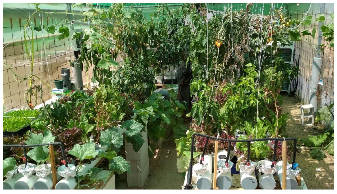
Two identical small-scale aquaponic systems (SAS1 and SAS2) based on FAO models were constructed using cheap and easy-to-obtain materials (recycling whenever possible) and monitored from the beginning of March 2018 to the end of April 2019. The SAS were placed inside a 9 × 5 m greenhouse located at the IES Joaquín Romero Murube secondary school (Seville, Spain; 37°21′30.4″ N, 5°58′19.8″ W) in the Polígono Sur neighborhood (Figure 1). The SAS specifics and their operation are described in Appendix A.
During the high temperature period, from 21 June to 15 October, the plastic roof of the greenhouse was replaced by 40% shade mesh. During the cold months (November to the middle of March), when the water temperature dropped below 20 °C, and until the end of this study (on 24 April 2019), two different strategies were employed to alleviate low system water temperatures.
In SAS1, a thermo-solar panel was coupled to the system in order to heat the water, so its temperature did not drop below 13 °C. When the temperature outside the greenhouse approached zero degrees, two submersible heaters were connected to the fish tank.
SAS2 did not work as an aquaponic system during cold months. The fish were removed and the plants were hydroponically grown using a nutrient solution (biofertilizer) obtained from a small vermicompost facility [29] installed next to the greenhouse.
2.2. Fish and Plant Species
Hybrid Oerochromis niloticus x Oerochromis mossambicus tilapia was selected as the fish species. The fish were obtained from the “Aula del Mar” hatchery (Málaga, Spain) 1–2 weeks after the absorption of the yolk-sac at a price of 0.30 € per fry and nursed at the School of Agricultural Engineering (University of Seville, Seville, Spain) for 118 days until they reached an average weight of 12 g and were then sold at a price of 0.788 € per fingerling to IES Joaquín Romero Murube secondary school, where they were grown in two SAS to at least 350 g.
A polyculture of 22 types of vegetables (see Table 1 in the Results section or Appendix B) was grown to provide a diversity of products sufficient for the adequate feeding of a family in terms of nutritional requirements. The seedlings were periodically purchased from commercial plant nurseries.
2.3. Cost-Benefit Analysis and Level of Commoditization
The actual costs of every component of each SAS were recorded in order to obtain the total installation costs. To do so, the initial investment was distributed over the lifespan of each component (calculated according to the manufacturer’s guidelines about service life), in order to obtain the depreciation costs (€ year−1). The labor costs involved in the construction of the facilities were considered as opportunity costs. The total running costs (specific costs and overheads) of the SAS were calculated monthly, including energy costs (electricity), plants (seedlings), fish (fingerlings), water, commercial fish food, additives and natural treatments for plants and water test kits.
The electricity supply was provided by ENDESA, with a minimum supply contract of 2.2 kW (the minimum power that can be contracted in Spain) (0.22 € kWh−1). The water was supplied by EMASESA (the public water company of Seville) (2 € m−3). The price of the seedlings varied depending on the plant species (0.05–0.10 € unit−1). The fish feed costs correspond to a purchase of 150 kg, also considering freight costs (1.41 € kg−1).
The time spent on each of the activities required for the maintenance and management of the systems was recorded to obtain the number of labor hours employed. These activities included measuring and regulating physical-chemical water parameters and the air temperature and observations of the health status of fish and plants, in addition to the water levels and flows, the replenishment of optimal water levels, treatments and corrections of plant deficiencies, the maintenance and cleaning of the equipment and the plant and fish management. The latter activity included the time to weigh the fish (once per month) and to harvest them, as well as the time for planting out the seedlings of the different species of plants into the systems and for the harvest of green leaves and fruits. Seedlings were purchased directly from commercial nurseries, so no time was used in managing plants from germination to seedlings.
The fish and plant production was recorded monthly to observe the periods of higher and lower production throughout the study year. Although, in this work, all the production was intended for family self-consumption, the economic value of the vegetable productions was obtained using market prices, under the assumptions of (a) production as substitution of purchased food in the self-consumption scenario and (b) use within the direct market chain in a potential selling scenario. Market prices were obtained monthly using the “origin and destination prices index” from the report offered by the Coordinator of Farmers and Livestock Organizations (COAG from the acronym in Spanish). Table A1 in Appendix B shows the monthly prices corresponding exclusively to the months in which each product was harvested. The total value of the horticultural production was calculated as the sum of the production of each of the vegetables multiplied by the average price (considering only the months in which each crop had been harvested).
Similarly, the economic value corresponding to the fish was obtained as an average of the unitary price of tilapia found in different local supermarkets: 9.6 € kg−1.
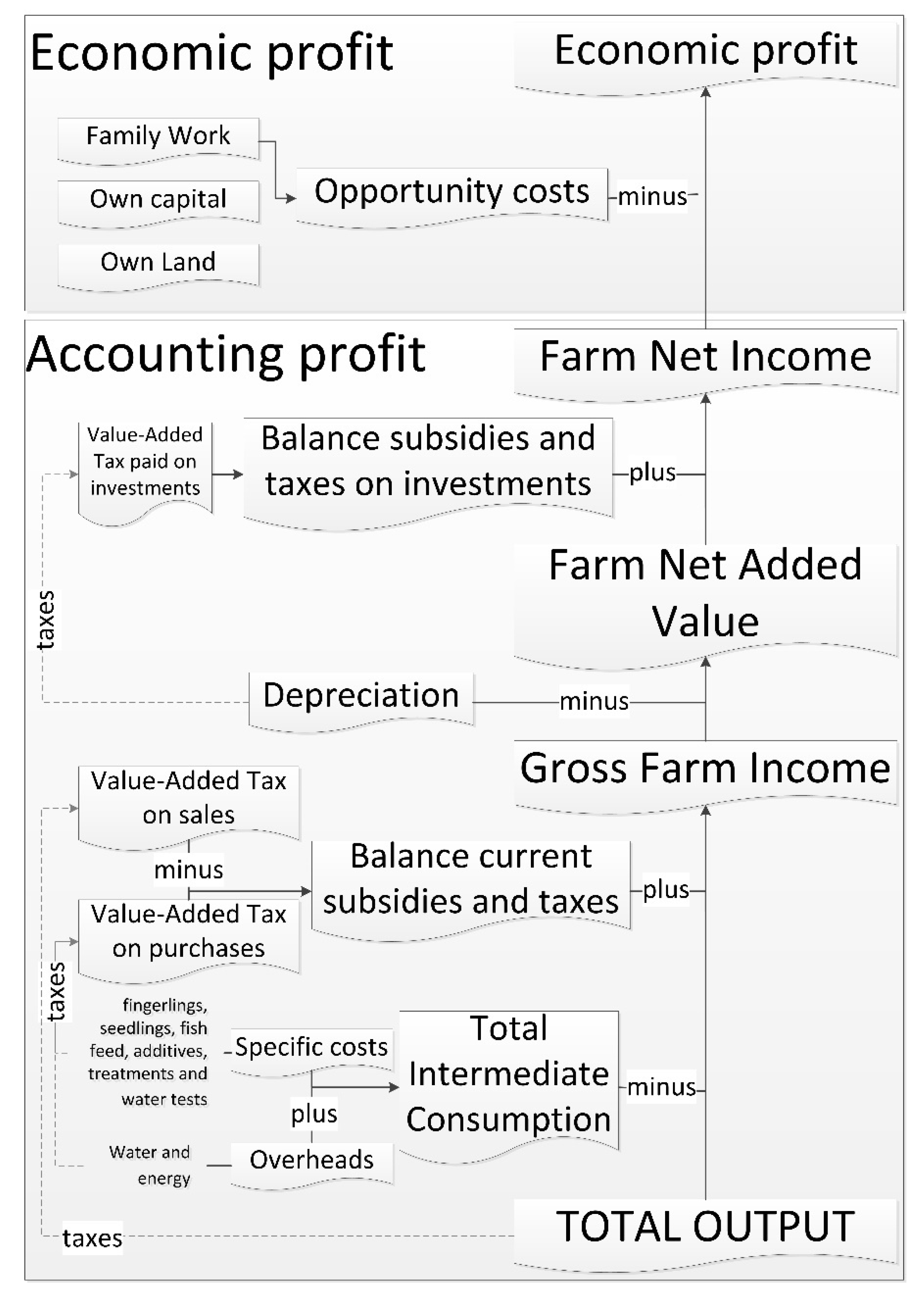
The cost-benefit analysis was based on two different approaches (Figure 2). On the one hand, the indicators of the farm accountancy data network (FADN) [30] were used in order to determine the farm net added value (FNAV) as an estimator of accounting profitability of systems (income less costs). FNAV is the most suitable indicator for domestic aquaponic systems, since external factors (wages, rents and interests paid) are not included. On the other hand, opportunity costs were included to calculate the economic profitability (income less costs and opportunity costs) from farm net income (FNI).
According to the FADN, FNAV is calculated through gross farm income (GFI) minus depreciation costs and including the balancing of current subsidies and taxes. Depreciation is estimated as the linear depreciation of replacement value over the lifespan of each component of the system separately (the closing value of components were not considered). Since this type of system does not receive subsidies, the balance of taxes only includes VAT (value added tax) on sales and purchases. GFI is the difference between the total output and the total intermediate consumption. In order to apply FADN requirements, the total output was computed as the value of production in the direct local market, despite the fact that self-consumption systems are considered a special case according to the Commission Regulation (EC) No. 1242/2008 of 8 December 2008 and standard outputs are regarded as equal to zero. The total output is the average market value of vegetables and fish produced in a year. Intermediate consumption includes specific costs (fingerlings, seedlings, fish feed, additives, treatments and water tests) and overheads (water and energy). In order to improve comparison with other studies, we included production value, running costs and depreciation costs that compute VAT (Table A2, Table A3 and Table A4 in Appendix B and Table 1) and output, intermediate consumption and depreciation (without VAT) (Table 2 in the results section).
The costs were classified as variable or fixed costs in the short term, since a one-year cycle was analyzed. Specific costs are variable and they depend on production, whereas overheads and depreciation are fixed costs and are not linked to production. The cost of one output unit is estimated as the total average cost, which included average fixed and variable costs.
Since the workforce was not remunerated, labor costs were included as opportunity costs according to the network of typical farms [31] and the agri benchmark analytical procedures [32]. They were calculated as the minimum salary that the workers did not receive because they were involved in system management (4.35 € h−1). Economic profitability allows for evaluating the capacity of the system to remunerate fixed factors according to the economic surroundings. Land and investment returns are considered as the interest of fixed capital and therefore their value is low because the current interest rate is low enough not to be included. The farm income (rate between family farm income and family work unit in full-time person equivalents) was included as a social indicator [33].
The level of commoditization was estimated as the rate between the marketized costs (all intermediate consumption in this study) and the total system costs (including family labor costs). Commoditization measures directly how the commodity market has penetrated within the systems and indirectly the degree of autonomy [34,35].
SAS were evaluated using economic profit as an indicator of their value as an alternative investment (whether the system is able to remunerate opportunity or implicit costs) [36] and through the farm net added value, which is an indicator of their capacity to remunerate fixed factors (work, land and capital) [30]. Moreover, we complemented the systems valuation with a cost analysis for a product competitiveness estimation (whether products could have a price low enough to be competitive in the markets) [37]. The degree of commoditization was also used as an indicator of farm autonomy [35].
3. Results
In order to assess the aquaponic production in economic terms, all the values for the investment in installations and equipment, depreciation, specific costs, overheads and labor costs and productions obtained were computed.
Table A2 in Appendix B shows the investment for the construction of SAS and the equipment required. The differences between the values corresponding to SAS1 and SAS2 are due to the additional investment for the solar panel installation and the vermicompost facility, respectively.
Table A3 and Table A4 in Appendix B show monthly and annual running costs for SAS1 and SAS2, respectively. Moreover, the percentage that each item represents of the total running costs is included. A total of 335.11 € was spent on the operation of SAS1, while 364.28 € was needed for SAS2 (294.27 € and 320.84 € of intermediate consumption for SAS1 and SAS2, respectively). Energy and fingerlings represent the main costs in both SAS, followed by fish feed and water colorimetric tests in SAS1 and additives for plants, water test kits and fish feed in SAS2. The seedlings, water and natural treatments against plant pests were minor costs.
In addition, a total of 99.9 h of labor (16.4 min on average each day) were spent for SAS1 maintenance and management during the year of study, while this was 120.8 h for SAS2 (19.8 min each day). Therefore, the opportunity costs of labor were 527.95 € and 618.81 €, respectively.
The average total monthly running costs for the total study period were 23.94 € month−1 ± 20.94 in SAS1 and 26.08 € month−1 ± 18.43 in SAS2.
The degree of commoditization of both systems is approximately 44% (44.8% and 43.1% for SAS1 and SAS2, respectively), which means that system reproduction depends on the part of the market which entails cash payments. However, an important share of the system depends on labor, which entails opportunity costs but not cash payments. Therefore, the SAS maintain a certain level of autonomy from the market thanks to the use of family labor forces as an internal resource.
For SAS1, the total horticultural production was nearly 180 kg, while 33.5 kg of fish were obtained (Table 1). The SAS2 production was slightly lower, with 175 kg of vegetables and nearly 30 kg of fish. The horticultural production was valued at 334.6 € and 327.0 € for SAS1 and SAS2, respectively (total output crops: 321.68 € and 318.07 €, respectively). The fish production would have a market value of 321.6 € and 281.0 € for SAS1 and SAS2, respectively (total output livestock: 292.36 € and 273.95 €, respectively). Therefore, the combined production of plant and fish would be around 632.0 € on average (total output: 603 €). Lettuce was by far the main vegetable produced, followed by tomatoes, cucumbers, peppers and zucchinis.
However, in terms of economic value, both lettuce and basil (the former due to its high production and the latter due to its high price) represented more than 10% of the total market value of the joint vegetable/fish production. Tomatoes, peppers and zucchinis also substantially contributed to the total value. Though the plant production represented around 85% of the total production, the fish production being 15%; in terms of economic value, the contributions were 52.3% and 47.7%, respectively.
The farm net added value was 181.10 € and 121.59 € for SAS1 and SAS2, respectively (Table 2). Therefore, both systems were able to remunerate fixed factors of production since they produced 1.41 € and 1.27 € per each euro spent (output/input rate). The difference between both systems is due to an increase of 7.5% in the SAS2′s total inputs, mainly related to higher overheads (28.7% higher in SAS2 in comparison with SAS1) and a decrease of 3.6% in the total output of SAS2 in comparison with SAS1.

Table 1.
Total horticultural and fish annual production (kg) and economic value of the production (€) per product in both aquaponic systems and average values (VAT included).
Table 1.
Total horticultural and fish annual production (kg) and economic value of the production (€) per product in both aquaponic systems and average values (VAT included).
| SAS | SAS1 | SAS2 | Average Values | |||||
|---|---|---|---|---|---|---|---|---|
| Produce | Total per Product (kg) | Total Market Value (€) | Total per Product (kg) | Total Market Value (€) | Total per Product (kg) | % of Total Production | Total Market Value (€) | % of Total Market Value |
| Lettuce | 68.72 | 70.09 | 64.54 | 65.83 | 66.63 | 32.1 | 67.96 | 10.8 |
| Watermelon | 4.90 | 4.31 | 1.65 | 1.45 | 3.28 | 1.6 | 2.88 | 0.5 |
| Chard | 9.33 | 19.78 | 7.31 | 15.50 | 8.32 | 4.0 | 17.64 | 2.8 |
| Raf tomato | 8.50 | 17.51 | 12.44 | 25.63 | 10.47 | 5.0 | 21.57 | 3.4 |
| Roma tomato | 14.16 | 26.20 | 12.48 | 23.09 | 13.32 | 6.4 | 24.64 | 3.9 |
| Eggplant | 3.34 | 6.01 | 10.16 | 18.29 | 6.75 | 3.3 | 12.15 | 1.9 |
| Cucumber | 18.52 | 26.48 | 20.34 | 29.09 | 19.43 | 9.4 | 27.78 | 4.4 |
| Basil | 1.78 | 71.20 | 1.61 | 64.40 | 1.70 | 0.8 | 67.80 | 10.7 |
| Onion | 0.06 | 0.07 | 0.06 | 0.07 | 0.06 | 0.0 | 0.07 | 0.0 |
| Italian frying pepper | 10.44 | 22.76 | 8.28 | 18.05 | 9.36 | 4.5 | 20.40 | 3.2 |
| Goat horn pepper | 2.02 | 4.24 | 1.51 | 3.17 | 1.77 | 0.9 | 3.71 | 0.6 |
| Lamuyo pepper | 4.66 | 11.09 | 3.86 | 9.19 | 4.26 | 2.1 | 10.14 | 1.6 |
| Broccoli | 2.92 | 6.92 | 1.77 | 4.19 | 2.35 | 1.1 | 5.56 | 0.9 |
| Strawberry | 0.75 | 2.64 | 0.79 | 2.78 | 0.77 | 0.4 | 2.71 | 0.4 |
| Cauliflower | 0.49 | 0.94 | 0.63 | 1.20 | 0.56 | 0.3 | 1.07 | 0.2 |
| Cabbage | 0.52 | 0.72 | 0.65 | 0.90 | 0.59 | 0.3 | 0.81 | 0.1 |
| Potato | 2.50 | 2.55 | 1.09 | 1.11 | 1.80 | 0.9 | 1.83 | 0.3 |
| Zucchini | 16.84 | 28.12 | 16.77 | 28.01 | 16.81 | 8.1 | 28.06 | 4.4 |
| Chinese cabbage | 1.73 | 3.39 | 1.79 | 3.51 | 1.76 | 0.8 | 3.45 | 0.5 |
| Stevia | 0.22 | 1.21 | 0.17 | 0.94 | 0.20 | 0.1 | 1.07 | 0.2 |
| Melon | 0.66 | 0.90 | 1.43 | 1.94 | 1.05 | 0.5 | 1.42 | 0.2 |
| Pumpkin | 4.63 | 7.41 | 5.44 | 8.70 | 5.04 | 2.4 | 8.06 | 1.3 |
| Total horticultural production | 177.66 | 334.55 | 174.77 | 327.04 | 176.22 | 84.9 | 330.79 | 52.3 |
| Tilapia | 33.50 | 321.60 | 29.28 | 281.09 | 31.39 | 15.1 | 301.34 | 47.7 |
Table 2.
Economic valuation of the two aquaponic systems. Total investment, farm net added value, economic profit, cost analysis, family farm income per family work unit and degree of commoditization.
Table 2.
Economic valuation of the two aquaponic systems. Total investment, farm net added value, economic profit, cost analysis, family farm income per family work unit and degree of commoditization.
| SAS1 | SAS2 | |
|---|---|---|
| Total investment | 2266.27 € | 2252.13 € |
| Total output livestock. Fish production | 292.36 € | 273.95 € |
| Total output crops. Plant production | 321.68 € | 318.07 € |
| Total output | 614.05 € | 592.01 € |
| Specific cost. Fingerlings, seedlings, fish feed, additives, treatments and water tests | 201.63 € | 201.59 € |
| Overheads. Water and energy | 92.64 € | 119.24 € |
| Intermediate consumption | 294.27 € | 320.84 € |
| Depreciation | 139.92 € | 144.06 € |
| Total inputs | 434.19 € | 464.9 € |
| Value added tax balance excluding on investments | 1.24 € | −5.52 € |
| Output/Input | 1.41 | 1.27 |
| Gross farm income | 321.02 € | 265.65 € |
| Farm net income | 151.72 € | 91.34 € |
| Annual work unit | 0.049 | 0.059 |
| Farm Net Added Value | ||
| 181.10 € | 121.59 € | |
| Economic Profit | ||
| −376.23 € | −527.47 € | |
| Costs Analysis | ||
| Variable costs (Specific costs) | 201.63 € | 201.59 € |
| Fixed costs (Value of labor, overheads and depreciation) | 668.13 € | 789.73 € |
| Total costs | 869.76 € | 991.32 € |
| Fish production | 33.25 kg | 29.28 kg |
| Plant production | 177.66 kg | 174.77 kg |
| Total production | 210.91 kg | 204.05 kg |
| Average cost per unit | 4.12 € kg−1 | 4.86 € kg−1 |
| Family Farm Income/FWU | ||
| 3090.41 € | 1539.50 € | |
| Degree of Commoditization | ||
| 44.8% | 43.1% | |
4. Discussion
The results shown above detail the different costs and revenues obtained by two SAS (with different strategies in the cold months). The initial investment per SAS was around 1643 € (1063 € excluding the greenhouse). Somerville et al. [9] estimated the initial investment to be around 700 US$ (527.11 €, considering the average exchange rate in 2014, when that study was performed) (they do not mention greenhouse investment or other means of protection for facilities), while Asciuto et al. [38] reported 1373 € (an outdoor system without a greenhouse). This obviously depends on the price of materials and the configuration of the system implemented.
In our study, the highest investment cost was the construction of the greenhouse (1160.63 € in materials plus the labor that was considered as opportunity costs). However, the greenhouse employed had a research/teaching purpose and was much bigger than necessary, in order to fit two SAS (and, hence, only the half of this investment cost was imputed to each SAS). A much less expensive greenhouse can be used for aquaponic production (though the production obtained could be different due to variations in the control capacity of climate control, and the lifespan of the greenhouse would be shorter).
Averages of monthly running costs for SAS1 (21.02 € month−1) and SAS2 (23.02 € month−1) are similar to those mentioned by Somerville et al. [9] for similar SAS for domestic use (26.45 € month−1). The annual running costs (335–364 €) and intermediate consumption (294–321 €) computed in our study are also in line with those suggested by Somerville et al. [9] and Asciuto et al. [38], who reported 318 U$ (239.46 €, 2014 exchange rate) and 437 €, respectively. In our case, energy represented one of the highest percentages of running costs (25.72% in SAS1, and 29.25% in SAS2), whereas Somerville et al. [9] and Asciuto et al. [38] did not find electricity costs so important (9.5% and 7%, respectively), while fish feed was considered the main cost (one of the highest also in our study). The energy price in the locations of the studies referred to can affect this distribution of costs. Hence, while in our study, the energy cost was 0.22 € per kWh, it was 0.10 € per kWh in Israel in 2014 and 0.16 € per kWh in Palermo (Italy) in 2019 (values corresponding to Somerville et al. [9] and Asciuto et al. [38], respectively). In Maucieri et al.’s study [7], electricity was also shown to be the most important factor in the life cycle analysis that they performed, so they suggested that efforts should be focused on reducing energy inputs. Here, again, Italy has a higher energy price (0.23 € per kWh in 2019 [39]).
In our study, the annual percentage of fingerlings is another of the highest costs (26.78% in SAS1 and 12.14% in SAS2) and is close to the 18.87% cited by Somerville et al. [9] as a percentage of the monthly running costs. This author cites a unit price for juvenile fish of 50 g of weight of 1 €. In Spain, a juvenile tilapia of this weight costs 3–4 €. For Asciuto et al. [38], this annual percentage was as low as 1.57%, mentioning a price of 0.05 € for each fry, while in Spain, the cost of a tilapia fry (1 week old) was 0.30 €, and growing it to 10–12 g involved 0.48 € more. The supply and prices of tilapia fingerlings or other fish species may be one of the factors that most limit the development of aquaponics in Spain, both for self-consumption and commercial use, a fact also mentioned by Hambrey et al. [40] and Sommerville [23].
The value of the annual horticultural production was estimated to be around 320 €, and 280 € for the tilapia production. Asciuto et al. [38] reported a revenue of 1350 € from lettuce production and 216 € from tilapia. The values determined by Somerville et al. [9] were 520 US$ (391.57 €) for vegetables (lettuce and tomato) and 240 US$ (180.72 €) for fish. In these two studies, the value of the horticultural production was higher than in ours, mainly due to the crops employed and higher market prices. Crop areas for plants were similar (4.56 m2 in our study, 5 m2 in Asciuto’s and 3 m2 in Somerville’s). Managing an aquaponic system with only one or two crops is always easier than polyculture (i.e., growing multiple plant species at the same time), because this requires the management of different nutrient needs and growing conditions for each plant species [41]. Furthermore, if a very productive crop in aquaponic conditions (for instance, using crops with shorter production cycles, such as lettuce) is used throughout the whole year, the production will be higher, as demonstrated in the aforementioned study of Asciuto et al. [38], which, in the monoculture of baby-leaf lettuces, managed an increase in annual production per m2. Obviously, if the products (either fish or plants) grown are in much demand in the market, and/or have high prices (such as stevia or basil), the revenues will be higher [42]. In the case of our study, the aim was to produce a variety of different products which can be consumed by the families operating the SAS, not to maximize the revenue using a productive or high-priced crop.
The region in which the aquaponic facility is located also influences both the costs (mainly energy but also depreciation and, if considered, labor) and the potential production obtained. In this regard, it is not the same to produce vegetables and tilapias in, for example, the Virgin Islands [2,42] as in Spain, mainly because of the hours of inbound radiation and the fluctuations in temperatures. These important limitations to aquaponics production have also been cited by Hambrey et al. [40] in the Pacific Islands.
Regarding the strategies that we employed for the cold months, heating the water using solar panels and stopping fish production (SAS1) by removing the fish and employing a nutrient solution from vermicompost (SAS2) were acceptable. Though energy costs were 20% lower in SAS2, more water (nearly 50% more) and labor hours (17.2% higher) were required. The difference in water consumption was due to the vermicompost facility and the need to change the nutrient solution often because of the excess of salinity. Vegetal production in the cold months in SAS2 (77.2 kg) was 8% lower than in SAS1 (83.83 kg). This fact, together with the lack of fish production during these months, resulted in a drop in the value of total production achieved. In terms of sustainability, the vermicompost facility enables the reuse of organic domestic waste (completely fitting circular economy principles) but, on the other hand, much more water is required.
The economic valuation of the two SAS shows a positive FNAV, which means a positive gain because annual outputs (the economic value of the fish and plant production) exceed the annual intermediate consumption and depreciation (Table 2). The output/input ratio was 1.41 and 1.27 for SAS1 and SAS2, respectively. These values are consistent with those provided by other authors. For instance, Sunny et al. [20] reported output/input ratios in Bangladesh between 1.90 and 2.2 and Goda et al. [19] between 1.17 and 1.53 in Egypt. Asciuto et al. [38] estimated an output/input ratio of 1.23 while Somerville et al. [9] gave a value of 1.38. The family farm income per family work unit was higher than the 2000 € reported by Ryś-Jurek [43] for small farms (year 2015) in the European Union.
The negative economic profit obtained (Table 2) means that revenues are lower than the sum of costs, depreciation and labor costs included as opportunity costs. Labor cost would result in an increment of costs of 157% in SAS1 and 169% in SAS2. This would lead to output/input ratios of 0.64 and 0.53, respectively, thus not being viable.
Although the farm net value added is positive, the economic profit is negative because non-paid family work cannot be fully remunerated in either system. As in the case of the farm net value added and the output/input rate, the economic profit is lower in SAS2 (the losses are 40.2% higher in SAS2) because the value of labor is 17.2% higher than SAS1, which required less work units.
Total inputs are higher in SAS2 than in SAS1, total costs being also 14.4% higher. Therefore, the average cost per unit was 17.8% higher in SAS2, since it was less productive than SAS1 (3.3%), mainly due to lower (11.9%) fish production. Therefore, SAS2 consumed more overheads and depreciation and required more work units, so the income per family work unit was 100.7% lower than SAS1.
The cost values of 4.12 € kg−1 in SAS1 and 4.86 € kg−1 in SAS2 are well below the market prices of fresh tilapia in Seville (8.7 € kg−1) and even frozen tilapia from China (about 5.5–6.4 € kg−1). In the case of plants, the production costs in SAS1 and SAS2 are above market prices (Table A1 in Appendix B) in all products except for stevia and basil, which provide less than 1% of total production.
From an economic point of view, systems produce economic losses because they are unable to remunerate the labor required. Under the assumption of maximizing benefits, purchasing products is preferable to producing them. However, non-valuable benefits could drive aquaponics, such as social and cultural services. Development and improvement strategies must combine classical profitability and social criteria (i.e., autonomy).
As for strategies to reduce intermediate consumption, the energy costs could be lowered using 12–24 V solar pumps connected to a photovoltaic panel. In any case, this would be a combined use of photovoltaic energy and the electricity grid, since the high price of batteries and their short lifespan probably does not compensate for the excessive increase of investment, either for an SAS or for some commercial aquaponic systems [44]. Eurythermal fish species could also be used for SAS in Southern Spain, in order to avoid using thermo-solar panels or heaters during cold months.
Another option to reduce costs would be the integration of aquaponic producers so that they can buy larger quantities of fry, fish feed or other supplies, reducing sale and shipping prices. This would also help to reduce the intermediate consumption (energy, water, etc.) if a common nursery is set up to grow the fry. Finally, the costs of water test kits can also be reduced after the first year of operation of an SAS once the farmer has had more training and hands-on experience.
Reducing the price of electricity (Spain has one of the most expensive electricity prices in the EU [45]) or of water is beyond the aquaponic farmer’s control. Another option is using well water, depending on the degree of contamination of the aquifers. Policy changes would be needed to achieve cheaper energy and water prices for food production.
In terms of revenue, it is possible to increase fish and plant production in both SAS if the management of fish biomass is optimized and the large amount of nutrients that are in the water over 4–5 months are better used [46].
Combined strategies could be considered at a family level, such as selling the production of one of the plant species at a good price (for example, basil) and using the money obtained to cover some of the expenses of the SAS or recover part of the investment.
Despite the negative economic profit of the two SAS, these types of systems could allow families to cope with failures of markets and incomes [25]. Autonomy is mainly based on the system’s low commoditization as a balance between internal and external resources. Thus, the use of self-managed SAS can be considered as a specific style of farming based on autonomy rather than on profitability through the balance between internal and external resources [35]. This suggests that many systems around the world show a negative economic profit because families are not forced to remunerate fixed factors at an average rate since the role of these factors is food production instead of providing gains.
Another aspect to consider is whether these systems should be valued only in economic terms such as industrial agricultural systems, where the scale or size of the farm plays an important role. Industrial agriculture is based on the economy of scale, in which the average cost of one product per unit falls as the scale of production increases, i.e., the more it is produced (up to certain levels), the less it costs to produce each unit [47]. Increasing size could mean increased productivity and profitability, but this does not occur on a smaller scale [48]. In the case of aquaponic systems, most studies that found a positive relationship between size and productivity were conducted with much larger aquaponic systems than those we have used in this study, even when the authors sometimes described them as small-scale systems [44].
In the case of familial agricultural systems, scale or size would not be so related to productivity or profitability but to the family’s ability to produce food according to non-economic factors such as autonomy, satisfaction, high-quality or pesticide-free foods. This is because many familial agricultural systems are not based on the economy of scale but on the economy of scope, where costs are reduced by optimally allocating resources and reusing them within the system [49]. In the case of aquaponic systems, the reuse of resources (fish waste nutrients) aims to improve system efficiency and reduce costs (in this case, avoiding the purchase of agricultural fertilizers). However, this way of improving efficiency does not compensate for the disadvantage of being small-scale [50].
The social potential of small-scale aquaponic production should also be mixed into the equation [16]. On the one hand, would people without financial resources have access to certain products if they did not produce them by themselves? On the other hand, the soft benefits procured by this activity (i.e., social cohesion, environmental awareness, education, leisure, psychological benefits) should also be valued.
Another non-monetizable aspect giving more added value to this kind of aquaponic system is the quality of the production [51], as products can be harvested at the demand of the consumer in their optimal state of maturation and consumed fresh the same day (without having to go through the chain of transport, conservation and storage of fresh products that are marketed) and are at the same time pesticide-free. There are many studies that show a greater willingness to consume food if it has been obtained through organic procedures or with added health and environmental values [52]. Although, according to current regulations, aquaponic products are not considered as “organic” in the EU [14], their above-mentioned characteristics (high quality and pesticide-free) are beginning to be taken into account by consumers when it comes to their willingness to pay and consume [53]. These added benefits can also play an important role in producer–consumer relations in smart cities [13].
5. Conclusions
Although SAS are popular in many countries at the family level for domestic food production, there are hardly any economic data on this type of aquaponic production, especially when destined to obtain a polyculture of vegetables. Hence, this study was aimed at producing economic reference information of this type of systems, considering the region’s climatic characteristics and limitations.
Overall, each of our SAS cost in average 1643 € to build, 350 € to operate annually and produced 632 € in equivalent value of food.
SAS showed a negative economic profit but positive accounting profit, because the family workforce is not paid but it entails opportunity costs in the case of domestic systems. In this context, the implementation of this type of system could be explained on the basis of other values and utilities, such as autonomy and the self-consumption of healthy products (high quality food, both fish and vegetables free of pesticides), as is proposed in our analysis. These values should be taken into account to implement strategies to develop SAS, complementing conventional criteria such as productivity and profitability. This is even more important in areas subjected to social exclusion and poverty.
However, further research must be carried out to analyze the value attributed to the autonomy gained and the contribution to a healthier diet, in order include them as additional variables to valorize this kind of food production.
Author Contributions
J.L.-E.: conceptualization, methodology, formal analysis, investigation, writing—original draft. V.M.F.-C.: conceptualization, methodology, formal analysis, writing—review and editing. L.A.B.: formal analysis, writing—review and editing. L.P.-U.: conceptualization, methodology, formal analysis, writing—original draft, writing—review and editing. All authors have read and agreed to the published version of the manuscript.
Funding
This research was not funded by any funding agency.
Acknowledgments
We are very grateful to the IES Joaquín Romero Murube secondary school for providing the location and for their willingness to help. We thank Manuel Alcón, Alberto Toriz and Alejandro Ponce for their assistance in maintaining aquaponic facilities during the harsh summer in Seville. Our thanks to the partners of the Aquaponics association “Plantío Chinampa”, especially to Javier Quevedo and Juan Manuel Selma, for sharing ideas and finding creative solutions. Finally, our gratitude to the Verdes del Sur association, especially Juan Manuel Blanco, and to the more than 200 patrons who made the project “The miracle of the fish” possible.
Conflicts of Interest
The authors declare no conflict of interest.
Appendix A. Aquaponic Systems’ Description and System Operations
The SAS consisted of a fish tank, connected to 3 hydroponic subsystems made up of a floating raft, a nutrient film technique (NFT) and a media bed that acted as a bio-filter, in addition to a clarifier and a sump (Figure A1).
Figure A1.
Schematics of the SAS: (1) fish tank; (2) clarifier; (3) biofilter and media bed; (4) sump and floating raft; (5) NFT. Blue arrows represent the direction of the water flows.
Figure A1.
Schematics of the SAS: (1) fish tank; (2) clarifier; (3) biofilter and media bed; (4) sump and floating raft; (5) NFT. Blue arrows represent the direction of the water flows.
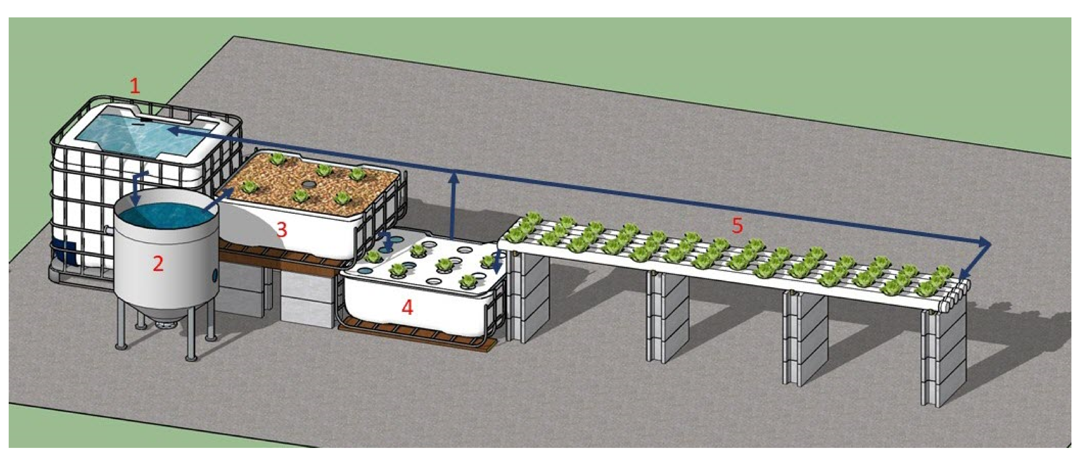
Fish were contained in prismatic (1.0 m × 1.2 m × 1.0 m) intermediate bulk containers (IBC) filled with 0.95 m3 of water. An air pump (5 W; 480 L h-1) was used for water aeration to ensure a correct level of dissolved oxygen in the fish tank.
Water was conducted by gravity from the fish tank to a conical clarifier with a total capacity of 400 L. From the clarifier the water flowed into an IBC tank cut in half with a capacity of 450 L filled with 300 L of pre-washed expanded clay. This tank worked as a biofilter and as a hydroponic subsystem (media bed) for the plant growth.
Afterwards, the water passed through a bell syphon to the sump tank with a capacity for 0.54 m3 (1 m × 1.2 m × 0.45 m). The sump had 1/3 of its surface area covered with 0.04 m thick extruded polystyrene foam (XPS) sheet (0.3 m × 1.2 m) with holes (0.05 m of diameter) that allowed placing three plants separated 0.25 m from each other (floating raft hydroponic subsystem). A submersible SunSun JTP 4800 32 W pump, placed inside the sump, sent 80% of the volume of the water back to the fish tank and the remaining 20% to the five PVC pipes which finally returned the water to the sump. These PVC pipes were part of the NFT hydroponic subsystem, made up of five 3 m long PVC pipes with a diameter of 0.11 m, separated 0.11 m from each other. They were placed on concrete blocks leveled to obtain a slope of 1%. Each pipe had 12 holes (0.05 m of diameter) separated 0.25 m from each other.
Before beginning to operate them, the SAS were subjected to a period of 40 days without fishes or plants, and an ammonia solution was added to the water, in order to allow the proliferation of nitrifying bacteria. Ammonia, nitrite and nitrate concentrations were monitored to check the nitrifying process until the end of the study.
In mid-April, the fish were placed in the SAS and the first vegetables were planted a week later. Minimum and maximum air temperatures inside and outside the greenhouse were monitored every day. The water consumption in the two SAS, both for the initial filling of the tanks and used to replenish water losses by evaporation and evapotranspiration, was registered. Water physical-chemical parameters, such as temperatures, the pH, concentration of dissolved oxygen, the electrical conductivity and nitrates, were periodically monitored and adjusted, if required. Water test kits (NO3 profi test SERA, TETRA test O2 and QP pH/chlorine test) were used to determine chemical parameters.
In order to maintain the optimal conditions and the well-being of the three biological populations (plants, fish and microorganisms) that cohabit in the SAS, some of the above parameters were adjusted in different ways, involving economic costs that were recorded. Calcium hydroxide was used to increase the pH when it dropped below 6-6.5. Optimal oxygen levels were maintained by venturi devices and air compressors. It was not necessary to regulate electrical conductivity or nitrate levels, which were always maintained at optimal levels.
The plants were periodically examined to observe the occurrence of nutrient deficiency and, when required, K2SO4 and MnSO4 at 1.5% were foliarly applied. A chelated iron solution (1%) was directly added to the water (EDDHA Sequestrene 138 Fe). These were included in the intermediate consumption as additives for plants. Other products were used for the treatment of possible pests that could appear in the plants and recorded in the intermediate consumption as treatments for plants.
The fishes were fed four times a day using pellets (Skretting TI-3 Tilapia compound feed, 32.6% of protein and 6% of fat). The amount of daily food was calculated as a percentage of the fish biomass, supplying between 1 and 4% of the total fish weight.
Appendix B. Economic Data
Table A1.
Horticultural crops grown in the SAS and market prices (€ kg−1) used each month for the produce obtained (VAT included).
Table A1.
Horticultural crops grown in the SAS and market prices (€ kg−1) used each month for the produce obtained (VAT included).
| Year | 2018 | 2019 | |||||||||||
|---|---|---|---|---|---|---|---|---|---|---|---|---|---|
| Month | May | June | July | Aug | Sep | Oct | Nov | Dec | Jan | Feb | Mar | April | Mean± SD |
| Lettuce | 0.97 | 0.97 | 0.99 | 1.01 | 1.04 | 1.05 | 1.05 | 1.03 | 1.09 | 1.06 | 0.97 | 1.02 ± 0.04 | |
| Water melon | 0.88 | 0.88 | |||||||||||
| Chard | 2.08 | 2.12 | 2.17 | 2.21 | 2.15 | 2.07 | 2.05 | 2.12 ± 0.06 | |||||
| Raf tomato | 2.03 | 2.03 | 2.11 | 2.06 ± 0.05 | |||||||||
| Roma tomato | 1.85 | 1.85 | 1.85 | 1.85 | |||||||||
| Eggplant | 1.58 | 1.58 | 1.93 | 1.94 | 1.95 | 1.80 ± 0.20 | |||||||
| Cucumber | 1.49 | 1.39 | 1.36 | 1.46 | 1.43 ± 0.06 | ||||||||
| Basil | 40 | 40 | 40 | 40 | 40 | 40 | 40 | 40.00 | |||||
| Onion | 1.17 | 1.17 | |||||||||||
| Italian frying pepper | 2.54 | 2.14 | 2.13 | 2.03 | 2.05 | 2.17 | 2.18 ± 0.19 | ||||||
| Goat horn pepper | 2.14 | 2.13 | 2.03 | 2.05 | 2.17 | 2.10 ± 0.06 | |||||||
| Lamuyo pepper | 2.4 | 2.39 | 2.35 | 2.39 | 2.38 ± 0.02 | ||||||||
| Broccoli | 2.45 | 2.4 | 2.27 | 2.37 ± 0.09 | |||||||||
| Strawberry | 3.87 | 3.6 | 3.45 | 3.15 | 3.52 ± 0.30 | ||||||||
| Cauliflower | 1.91 | 1.91 | |||||||||||
| Cabbage | 1.43 | 1.35 | 1.39 ± 0.06 | ||||||||||
| Potato | 1.02 | 1.02 | |||||||||||
| Zucchini | 1.63 | 1.71 | 1.67 ± 0.06 | ||||||||||
| Chinese cabbage | 1.96 | 1.93 | 1.98 | 1.96 ± 0.03 | |||||||||
| Stevia | 5.5 | 5.5 | 5.5 | 5.5 | 5.50 | ||||||||
| Melon | 1.29 | 1.43 | 1.36 ± 0.10 | ||||||||||
| Pumpkin | 1.6 | 1.6 | 1.60 | ||||||||||
Table A2.
Construction and equipment costs for the SAS (VAT included).
| Item | Total Cost (€) | Annual Cost (Depreciation) (€ year−1) |
|---|---|---|
| Greenhouse | 580.321 | 58.03 |
| Shade mesh | 25 | 5 |
| Electrical installation | 45 | 2.25 |
| Fish tank and related equipment | 182.75 | 19.85 |
| Tank for water refill | 54 | 5.40 |
| Clarifier | 166 | 10.32 |
| Biofilter and expanded clay growing bed | 86 | 8.93 |
| NFT system | 69 | 7.5 |
| Sump & pump | 137 | 19.02 |
| Accessories | 57.90 | 17.07 |
| Solar panel and related equipment (only for SAS1) | 247.55 | 15.93 |
| Vermicompost facility (only for SAS2) | 181.91 | 8.62 |
| Vermicompost accessories (only for SAS2) | 51.50 | 12.33 |
| Total cost for SAS1 | 1650.52 | 169.30 |
| Total cost for SAS2 | 1636.38 | 174.32 |
Half of the total cost of the greenhouse was allocated to each of the two SAS.
Table A3.
Monthly (€ month-1) and annual (€ year-1) running costs for SAS1. Percentage of each input of the total (%) (VAT included).
Table A3.
Monthly (€ month-1) and annual (€ year-1) running costs for SAS1. Percentage of each input of the total (%) (VAT included).
| Year | 2018 | 2019 | Annual Cost | % over Total | ||||||||||||
|---|---|---|---|---|---|---|---|---|---|---|---|---|---|---|---|---|
| Month | March | April | May | June | July | Aug | Sep | Oct | Nov | Dec | Jan | Feb | Mar | April | ||
| Energy costs (electricity) | 3.17 | 3.52 | 4.37 | 4.92 | 6.07 | 5.98 | 6.07 | 6.23 | 6.83 | 9.16 | 15.80 | 7.36 | 6.81 | 5.27 | 91.57 | 27.33 |
| Fish (fingerlings) | 86.68 | 86.68 | 25.86 | |||||||||||||
| Plants (seedlings) | 0.95 | 0.85 | 1.25 | 2.15 | 0.60 | 3.15 | 2.05 | 2.65 | 0.60 | 2.60 | 0.30 | 3.25 | 0.00 | 20.40 | 6.09 | |
| Fish feed | 1.39 | 4.44 | 6.53 | 9.91 | 11.02 | 7.50 | 6.82 | 2.45 | 2.40 | 1.09 | 1.13 | 3.41 | 2.64 | 60.72 | 18.12 | |
| Water | 1.52 | 1.00 | 1.80 | 3.00 | 3.44 | 2.13 | 1.06 | 0.52 | 0.80 | 0.15 | 0.95 | 1.17 | 1.12 | 18.66 | 5.57 | |
| Additives for plants | 0.06 | 0.31 | 0.33 | 0.06 | 0.07 | 0.39 | 0.13 | 0.12 | 0.23 | 0.35 | 0.45 | 0.24 | 0.25 | 2.97 | 0.89 | |
| Treatments for plants | 0.34 | 0.34 | 0.43 | 0.74 | 1.14 | 3.34 | 0.55 | 0.03 | 0.03 | 6.95 | 2.07 | |||||
| Water tests | 0.40 | 2.03 | 3.67 | 3.74 | 4.48 | 8.56 | 4.82 | 4.88 | 3.32 | 2.75 | 2.05 | 1.80 | 2.57 | 2.12 | 47.18 | 14.08 |
| Monthly running costs | 5.08 | 94.62 | 14.64 | 18.57 | 26.01 | 30.02 | 24.49 | 21.90 | 17.04 | 19.27 | 22.58 | 11.98 | 17.49 | 11.42 | 335.11 | |
Table A4.
Monthly (€ month-1) and annual (€ year-1) running costs for SAS2. Percentage of each input of the total (%) (VAT included).
Table A4.
Monthly (€ month-1) and annual (€ year-1) running costs for SAS2. Percentage of each input of the total (%) (VAT included).
| Year | 2018 | 2019 | Annual Cost | % over Total | ||||||||||||
|---|---|---|---|---|---|---|---|---|---|---|---|---|---|---|---|---|
| Month | March | April | May | June | July | Aug | Sep | Oct | Nov | Dec | Jan | Feb | Mar | April | ||
| Energy costs (electricity) | 3.17 | 3.38 | 4.48 | 5.28 | 6.33 | 6.16 | 6.07 | 6.46 | 5.90 | 4.91 | 5.25 | 5.45 | 5.85 | 4.51 | 73.2 | 20.09 |
| Fish (fingerlings) | 81.96 | 43.79 | 22.50 | |||||||||||||
| Plants (seedlings) | 1.00 | 0.80 | 1.25 | 2.10 | 0.55 | 3.15 | 1.90 | 2.65 | 0.65 | 2.75 | 0.20 | 3.05 | 20.05 | 5.50 | ||
| Fish feed | 1.45 | 4.27 | 6.57 | 10.29 | 10.92 | 7.55 | 6.11 | 47.15 | 12.94 | |||||||
| Water | 1.48 | 1.00 | 1.80 | 3.10 | 3.53 | 2.19 | 1.04 | 1.33 | 2.11 | 2.62 | 2.05 | 2.94 | 2.76 | 27.95 | 7.67 | |
| Additives for plants | 0.06 | 0.31 | 0.37 | 0.06 | 0.07 | 0.39 | 0.13 | 3.37 | 7.46 | 13.11 | 8.36 | 12.50 | 12.55 | 58.74 | 16.12 | |
| Treatments for plants | 0.34 | 0.34 | 0.43 | 0.74 | 1.14 | 3.34 | 0.55 | 0.03 | 0.03 | 6.94 | 1.91 | |||||
| Water tests | 0.40 | 2.03 | 3.67 | 3.74 | 4.48 | 8.56 | 4.82 | 4.88 | 5.21 | 3.81 | 2.37 | 2.13 | 2.20 | 0.03 | 48.32 | 13.26 |
| Monthly running costs | 5.04 | 89.85 | 14.53 | 19.01 | 26.70 | 30.13 | 24.59 | 21.25 | 19.60 | 22.27 | 26.65 | 18.18 | 26.57 | 19.88 | 364.28 | |
References
- König, B.; Janker, J.; Reinhardt, T.; Villarroel, M.; Junge, R. Analysis of aquaponics as an emerging technological innovation system. J. Clean. Prod. 2018, 180, 232–243. [Google Scholar] [CrossRef] [Green Version]
- Rakocy, J.E.; Masser, M.P.; Losordo, T.M. Recirculating aquaculture tank production systems: Aquaponics-integrating fish and plant culture. SRAC Publ. South. Reg. Aquac. Cent. 2006, 454, 1–16. [Google Scholar]
- Calone, R.; Pennisi, G.; Morgenstern, R.; Sanyé-Mengual, E.; Lorleberg, W.; Dapprich, P.; Winkler, P.; Orsini, F.; Gianquinto, G. Improving water management in European catfish recirculating aquaculture systems through catfish-lettuce aquaponics. Sci. Total Environ. 2019, 687, 759–767. [Google Scholar] [CrossRef] [PubMed]
- Delaide, B.; Teerlinck, S.; Decombel, A.; Bleyaert, P. Effect of wastewater from a pikeperch (Sander lucioperca L.) recirculated aquaculture system on hydroponic tomato production and quality. Agric. Water Manag. 2019, 226, 105814. [Google Scholar] [CrossRef]
- Palm, H.W.; Knaus, U.; Appelbaum, S.; Goddek, S.; Strauch, S.M.; Vermeulen, T.; Jijakli, M.H.; Kotzen, B. Towards commercial aquaponics: A review of systems, designs, scales and nomenclature. Aquac. Int. 2018, 26, 813–842. [Google Scholar] [CrossRef]
- Love, D.C.; Fry, J.P.; Li, X.; Hill, E.S.; Genello, L.; Semmens, K.; Thompson, R.E. Commercial aquaponics production and profitability: Findings from an international survey. Aquaculture 2015, 435, 67–74. [Google Scholar] [CrossRef] [Green Version]
- Maucieri, C.; Forchino, A.A.; Nicoletto, C.; Junge, R.; Pastres, R.; Sambo, P.; Borin, M. Life cycle assessment of a micro aquaponic system for educational purposes built using recovered material. J. Clean. Prod. 2018, 172, 3119–3127. [Google Scholar] [CrossRef]
- Maucieri, C.; Nicoletto, C.; Zanin, G.; Birolo, M.; Trocino, A.; Sambo, P.; Borin, M.; Xiccato, G. Effect of stocking density of fish on water quality and growth performance of European Carp and leafy vegetables in a low-tech aquaponic system. PLoS ONE 2019, 14, e0217561. [Google Scholar] [CrossRef] [Green Version]
- Somerville, C.; Cohen, M.; Pantanella, E.; Stankus, A.; Lovatelli, A. Small-Scale Aquaponic Food Production: Integrated Fish and Plant Farming; FAO Fisheries and Aquaculture Technical Paper 589; Food and Agriculture Organization of the United Nations: Rome, Italy, 2014; ISBN 9789251085332. [Google Scholar]
- Menon, R. Small Scale Aquaponic System. Int. J. Agric. Food Sci. Technol. 2013, 4, 2249–3050. [Google Scholar]
- Maucieri, C.; Nicoletto, C.; Schmautz, Z.; Sambo, P.; Komives, T.; Borin, M.; Junge-Berberovic, R. Vegetable Intercropping in a Small-Scale Aquaponic System. Agronomy 2017, 7, 63. [Google Scholar] [CrossRef]
- Pérez-Urrestarazu, L.; Lobillo-Eguíbar, J.; Fernández-Cañero, R.; Fernández-Cabanás, V.M. Suitability and optimization of FAO’s small-scale aquaponics systems for joint production of lettuce (Lactuca sativa) and fish (Carassius auratus). Aquac. Eng. 2019, 85, 129–137. [Google Scholar] [CrossRef]
- Dos Santos, M.J.P.L. Smart cities and urban areas—Aquaponics as innovative urban agriculture. Urban For. Urban Green. 2016, 20, 402–406. [Google Scholar] [CrossRef]
- Junge-Berberovic, R.; König, B.; Villarroel, M.; Komives, T.; Jijakli, M.H. Strategic Points in Aquaponics. Water 2017, 9, 182. [Google Scholar] [CrossRef] [Green Version]
- Csortan, G.; Ward, J.D.; Koth, B. Aquaponics in Urban Agriculture: Social Acceptance and Urban Food Planning. Horticulturae 2017, 3, 39. [Google Scholar] [CrossRef] [Green Version]
- Konig, B.; Junge, R.; Bittsanszky, A.; Villarroel, M.; Komives, T. On the sustainability of aquaponics. Ecocycles 2016, 2, 26–32. [Google Scholar] [CrossRef] [Green Version]
- Greenfeld, A.; Becker, N.; McIlwain, J.; Fotedar, R.; Bornman, J.F. Economically viable aquaponics? Identifying the gap between potential and current uncertainties. Rev. Aquac. 2018, 11, 848–862. [Google Scholar] [CrossRef]
- Ako, H.; Baker, A. Small-Scale Lettuce Production with Hydroponics or Aquaponics. Sustain. Agric. 2009, SA-2, 1–7. [Google Scholar]
- Goda, A.M.A.-S.; Essa, M.A.; Hassaan, M.S.; Sharawy, Z. Bio Economic Features for Aquaponic Systems in Egypt. Turkish J. Fish. Aquat. Sci. 2015, 15, 525–532. [Google Scholar] [CrossRef]
- Sunny, A.R.; Islam, M.M.; Rahman, M.; Miah, M.Y.; Mostafiz, M.; Islam, N.; Hossain, M.Z.; Chowdhury, M.A.; Islam, M.A.; Keus, H.J. Cost effective aquaponics for food security and income of farming households in coastal Bangladesh. Egypt. J. Aquat. Res. 2019, 45, 89–97. [Google Scholar] [CrossRef]
- Quagrainie, K.K.; Flores, R.M.V.; Kim, H.-J.; McClain, V. Economic analysis of aquaponics and hydroponics production in the U.S. Midwest. J. Appl. Aquac. 2017, 30, 1–14. [Google Scholar] [CrossRef]
- Xie, K.; Rosentrater, K. Life cycle assessment (LCA) and Techno-economic analysis (TEA) of tilapia-basil aquaponics. In Proceedings of the 2015 ASABE International Meeting, New Orleans, LA, USA, 26–29 July 2015; Volume 3, pp. 2248–2277. [Google Scholar]
- Somerville, C. Rooftop aquaponics for family nutrition in the Gaza strip, Palestine. In Rooftop Urban Agriculture; Orsini, F., Dubbeling, M., de Zeeuw, H., Gianquinto, G., Eds.; Springer: Berlin/Heidelberg, Germany, 2017; pp. 344–354. [Google Scholar]
- Ellis, F. Livelihoods and Diversity in Developing Countries; Oxford University Press: Oxford, UK, 2000; ISBN 0198296967. [Google Scholar]
- Schneider, S.; Niederle, P.A. Resistance strategies and diversification of rural livelihoods: The construction of autonomy among Brazilian family farmers. J. Peasant. Stud. 2010, 37, 379–405. [Google Scholar] [CrossRef]
- Van Der Ploeg, J.D. The peasantries of the twenty-first century: The commoditisation debate revisited. J. Peasant. Stud. 2010, 37, 1–30. [Google Scholar] [CrossRef]
- Milliken, S.; Stander, H. Aquaponics and Social Enterprise. In Aquaponics Food Production Systems; Springer Science and Business Media LLC.: Berlin/Heidelberg, Germany, 2019; pp. 607–619. [Google Scholar]
- INE. Indicadores Urbanos. Available online: https://www.ine.es/prensa/ua_2019.pdf (accessed on 27 August 2019).
- Dasgan, H.; Cetinturk, T.; Altuntas, O. The effects of biofertilisers on soilless organically grown greenhouse tomato. Acta Hortic. 2017, 555–561. [Google Scholar] [CrossRef]
- FADN. Farm Accounting Data Network An A to Z of Methodology. Available online: https://ec.europa.eu/agriculture/rica/pdf/site_en.pdf (accessed on 4 March 2020).
- Ministerio de Agricultura, Pesca y Alimentación. Análisis Comparativo de Costes Ligados al Modelo Europeo de Producción; Ministerio de Agricultura, Pesca y Alimentación: Madrid, España, 2019.
- Agri benchmark. Glossary of Terms Used in Agri Benchmark. Available online: http://www.agribenchmark.org/fileadmin/Dateiablage/B-Beef-and-Sheep/Misc/Other-Articles-Papers/BSR15-glossary.pdf (accessed on 10 December 2019).
- dos Santos, M.J.P.L.; Diz, H. Towards sustainability in European agricultural firms. Adv. Intell. Syst. Comput. 2019, 783, 161–168. [Google Scholar] [CrossRef]
- Friedmann, H. Household production and the national economy: Concepts for the analysis of Agrarian formations. J. Peasant. Stud. 1980, 7, 158–184. [Google Scholar] [CrossRef]
- van der Ploeg, J.D. Peasants and the Art of Farming; Practical Action Publishing: Warwickshire, UK, 2013; ISBN 978-1552665657. [Google Scholar]
- Dudin, M.N.; Lyasnikov, N.V.; Reshetov, K.Y.; Smirnova, O.O.; Vysotskaya, N.V. Economic Profit as Indicator of Food Retailing Enterprises’ Performance. Eur. Res. Stud. J. 2018, XXI, 468–479. [Google Scholar]
- Tynchenko, V.S.; Fedorova, N.V.; Kukartsev, V.V.; Boyko, A.A.; Stupina, A.A.; Danilchenko, Y.V. Methods of developing a competitive strategy of the agricultural enterprise. IOP Conf. Ser. Earth Environ. Sci. 2019, 315, 022105. [Google Scholar] [CrossRef]
- Asciuto, A.; Schimmenti, E.; Cottone, C.; Borsellino, V. A financial feasibility study of an aquaponic system in a Mediterranean urban context. Urban For. Urban Green. 2019, 38, 397–402. [Google Scholar] [CrossRef]
- EUROSTAT. Electricity Price Statistics—Statistics Explained. Available online: https://ec.europa.eu/eurostat/statistics-explained/index.php/Electricity_price_statistics (accessed on 9 September 2020).
- Hambrey, J.; Evans, S.; Pantanella, E. The Relevance of Aquaponics to the New Zealand aid Programme, Particularly in the Pacific; Ministry of Foreign Affairs and Trade (New Zealand): Wellington, New Zealand, 2013.
- Lennard, W. Aquaponic System Design Parameters: Fish to Plant Ratios (Feeding Rate Ratios). Aquaponics Solut. 2012, 3, 1–14. [Google Scholar]
- Bailey, D.S.; Ferrarezi, R.S. Valuation of vegetable crops produced in the UVI Commercial Aquaponic System. Aquac. Rep. 2017, 7, 77–82. [Google Scholar] [CrossRef]
- Ryś-Jurek, R. Family farm income and their production and economic determinants according to the economic size in the EU countries in 2004–2015. In Economic Sciences for Agribusiness and Rural Economy, Proceedings of the 2018 International Scientific Conference, Warsaw, Poland, 7–8 June 2018; No 2; Gołębiewski, J., Ed.; Warsaw University of Life Sciences Press: Warsaw, Poland, 2018; pp. 21–28. [Google Scholar]
- Tokunaga, K.; Tamaru, C.; Ako, H.; Leung, P. Economics of Small-scale Commercial Aquaponics in Hawai‘i. J. World Aquac. Soc. 2015, 46, 20–32. [Google Scholar] [CrossRef]
- European Commission. Energy Prices and Costs in Europe. Available online: https://ec.europa.eu/energy/sites/ener/files/epc_report_final_1.pdf (accessed on 5 March 2020).
- Nicoletto, C.; Maucieri, C.; Mathis, A.; Schmautz, Z.; Komives, T.; Sambo, P.; Junge-Berberovic, R. Extension of Aquaponic Water Use for NFT Baby-Leaf Production: Mizuna and Rocket Salad. Agronomy 2018, 8, 75. [Google Scholar] [CrossRef] [Green Version]
- Upchurch, M.L. Implications of Economies of Scale to National Agricultural Adjustments. J. Farm Econ. 1961, 43, 1239–1246. [Google Scholar] [CrossRef] [Green Version]
- Muyanga, M.; Jayne, T.S. Revisiting the Farm Size-Productivity Relationship Based on a Relatively Wide Range of Farm Sizes: Evidence from Kenya. Am. J. Agric. Econ. 2019, 101, 1140–1163. [Google Scholar] [CrossRef]
- Panzar, J.C.; Willig, R.D. Economies of Scope. Am. Econ. Rev. 1981, 71, 268. [Google Scholar]
- Shaik, S.; Addey, K.; Yeboah, O. Efficiency gains due to economies of scope and scale. In Proceedings of the 2017 Annual Meeting of Southern Agricultural Economics Association (SAEA), Mobile, Atlanta, 4–7 February 2017. [Google Scholar]
- Greenfeld, A.; Becker, N.; Bornman, J.F.; Dos Santos, M.J.; Angel, D. Consumer preferences for aquaponics: A comparative analysis of Australia and Israel. J. Environ. Manag. 2020, 257, 109979. [Google Scholar] [CrossRef]
- Rödiger, M.; Hamm, U. How are organic food prices affecting consumer behaviour? A review. Food Qual. Prefer. 2015, 43, 10–20. [Google Scholar] [CrossRef]
- Blidariu, F.; Grozea, A. Increasing the economical efficiency and sustainability of indoor fish farming by means of aquaponics. Anim. Sci. Biotechnol. 2011, 44, 1–8. [Google Scholar]
Figure 1.
Small-scale aquaponic systems located at the IES Joaquín Romero Murube secondary school (Seville, Spain) in full production.
Figure 1.
Small-scale aquaponic systems located at the IES Joaquín Romero Murube secondary school (Seville, Spain) in full production.

Figure 2.
Diagram of the farm accountancy data network (FADN) methodology employed for the cost-benefit analysis.
Figure 2.
Diagram of the farm accountancy data network (FADN) methodology employed for the cost-benefit analysis.

© 2020 by the authors. Licensee MDPI, Basel, Switzerland. This article is an open access article distributed under the terms and conditions of the Creative Commons Attribution (CC BY) license (http://creativecommons.org/licenses/by/4.0/).
Share and Cite
MDPI and ACS Style
Lobillo-Eguíbar, J.; Fernández-Cabanás, V.M.; Bermejo, L.A.; Pérez-Urrestarazu, L. Economic Sustainability of Small-Scale Aquaponic Systems for Food Self-Production. Agronomy 2020, 10, 1468. https://doi.org/10.3390/agronomy10101468
AMA Style
Lobillo-Eguíbar J, Fernández-Cabanás VM, Bermejo LA, Pérez-Urrestarazu L. Economic Sustainability of Small-Scale Aquaponic Systems for Food Self-Production. Agronomy. 2020; 10(10):1468. https://doi.org/10.3390/agronomy10101468
Chicago/Turabian StyleLobillo-Eguíbar, José, Víctor M. Fernández-Cabanás, Luis Alberto Bermejo, and Luis Pérez-Urrestarazu. 2020. "Economic Sustainability of Small-Scale Aquaponic Systems for Food Self-Production" Agronomy 10, no. 10: 1468. https://doi.org/10.3390/agronomy10101468
Note that from the first issue of 2016, this journal uses article numbers instead of page numbers. See further details here.