Linear Programming for Computing Equilibria Under Truncation Selection and Designing Defensive Strategies Against Malicious Opponents

Abstract

Linear programming and polyhedral representation conversion methods have been widely applied to game theory to compute equilibria. Here, we introduce new applications of these methods to two game-theoretic scenarios in which players aim to secure sufficiently large payoffs rather than maximum payoffs. The first scenario concerns truncation selection, a variant of the replicator equation in evolutionary game theory where players with fitnesses above a threshold survive and reproduce while the remainder are culled. We use linear programming to find the sets of equilibria of this dynamical system and show how they change as the threshold varies. The second scenario considers opponents who are not fully rational but display partial malice: they require a minimum guaranteed payoff before acting to minimize their opponent’s payoff. For such cases, we show how generalized maximin procedures can be computed with linear programming to yield improved defensive strategies against such players beyond the classical maximin approach. For both scenarios, we provide detailed computational procedures and illustrate the results with numerical examples.

1. Introduction

Game theory plays an important role in mathematically modeling the behavior and decision-making of players whether, or not they are human (Myerson, 1991). This feature allows the theory to have applications in fields such as social sciences, economics, biology, and computer science. In particular, many studies have focused on two-player games, which are an essential foundation of many models of interactions between individuals. As the size of players’ strategy sets increases, however, analyzing (say, finding the Nash equilibria) the multi-variable polynomial payoff expressions becomes computationally complex (Etessami & Yannakakis, 2010; Papadimitriou, 2007). In such situations, support enumeration is a standard approach to finding Nash equilibria (Dickhaut & Kaplan, 1993; Porter et al., 2008; Von Stengel, 2021). Linear programming can be used as an auxiliary tool for support enumeration and has been well applied to game theory (Lucchetti, 2006; Parrilo, 2006; Thie & Keough, 2011), often to compute minimax/maximin strategies, Nash equilibria, correlated equilibria, and related solution concepts. In this study, we convert problems into linear programs (or, more fundamentally, polyhedral conversion problems) and apply them to two additional scenarios: truncation selection and opponents that show a degree of irrationality or malice. We focus on these two scenarios because they both require consideration of worst-case scenarios, and they can be naturally expressed in linear algebraic language and converted to linear programs.

Before addressing irrational or malicious opponents, we begin with a discussion of rationality. In classical game theory, particularly for finite normal-form games, stable outcomes of games are predicted by Nash equilibria (Nash, 1950) (and its variants), which rely on at least two assumptions: that payoff matrices accurately and quantitatively reflect what matters to each player, and that all players aim to maximize their payoffs. In practice, however, players cannot always assume that their opponents are rational and must instead make decisions based on payoffs for all possible scenarios. For example, players may encounter opponents that are satisficers (Simon, 1955), irrational (Htun, 2005), unfamiliar with the game (Burton-Chellew et al., 2016), prone to making errors (Selten & Bielefeld, 1988), or malicious (Moscibroda et al., 2009). Another typical reason for the assumption of rationality to fail is that, in practice, payoff matrices usually only reflect the material payoffs of players, failing to capture players’ complicated underlying emotions. In the case of maliciousness, players may attempt to decrease their opponent’s payoff on purpose rather than maximize their own payoff. Such behavior can be explained by social norms that promote costly punishment (Henrich et al., 2006), a component of relational utility in a player’s payoffs (Su & Morsky, 2024), or the game being a sub-game of a larger game where opponents’ payoffs negatively affect one another. Players may also encounter games with incomplete information, such as Bayesian games (Harsanyi, 1968), where analyzing an opponent’s behavior with certainty is impossible. In controlling industrial scenarios, we may only seek satisfactory outcomes rather than optimal ones, especially if the optimization is difficult. In such situations, players may wish to guarantee themselves a minimum payoff (Bruyere et al., 2014)—i.e., control for worst-case scenarios (Dave & Malikopoulos, 2024).

Risk-averse or security strategies to handle such scenarios have been well studied (Binmore, 1992; Holler, 1990, 1992; Holler & Høst, 2019). A classic example is the maximin strategy, where a player assumes the worst-case scenario will happen and chooses a strategy that maximizes their payoff under that assumption. However, players may seek a balance between securing a lower-bound payoff and exploiting an opponent’s partial rationality. A safe equilibrium formalizes this trade-off by each player assigning probabilities over maximin and Nash equilibrium strategies (Ganzfried, 2023). When a player is willing to accept a worst-case payoff below the maximin value, they can respond more flexibly to educated beliefs about opponents’ behaviors. This flexibility may lead to higher payoffs, particularly when combined with methods in behavioral game theory (Fudenberg & Liang, 2019; Wright & Leyton-Brown, 2014). In this paper, we design a model to capture the behavior of partially malicious players: players who aim to increase their payoffs when they are low but become malicious once they exceed a certain payoff threshold. While a fully malicious player reduces the problem to a classic zero-sum game, our framework generalizes this case to opponents exhibiting partial malice. We demonstrate how a rational player can enhance their payoff from the maximin payoff if the opponent follows such a decision rule, and how such players would compute their ideal strategies. We analyze strategies for both rational players facing partially malicious opponents and malicious players seeking to minimize their opponents’ payoffs under this decision rule.

The population-level dynamics of avoiding worst-case outcomes can be modeled by truncation selection, an evolutionary algorithm in which only players with fitnesses (i.e., average payoffs) above a specified threshold survive and reproduce (Ficici, 2006; Ficici et al., 2005; Ficici & Pollack, 2000, 2007; D. B. Fogel et al., 1997; G. B. Fogel et al., 1998; G. B. Fogel & Fogel, 2011; Jebari & Madiafi, 2013; Morsky & Bauch, 2016, 2019). Thresholds may be fixed or dynamic and can depend on variables such as time, which is relevant for reproduction timing (Morsky et al., 2020). Truncation selection emphasizes adequacy: as long as a player’s fitness exceeds the threshold, they propagate at an equal rate. This approach has applications in computer science and mathematical biology, including genetic algorithms (Jebari & Madiafi, 2013) and as an alternative to the replicator equation (Morsky & Bauch, 2016). Truncation selection can exhibit markedly different dynamics than the replicator equation (D. B. Fogel et al., 1997), where population change depends on deviations from the average fitness (Cressman & Tao, 2014). Truncation selection can be classified into two different methods: independent truncation selection, where the threshold is a fixed value; and dependent truncation selection, where a fixed proportion of the population survives, making the threshold contingent upon the population’s fitness distribution (Morsky & Bauch, 2016, 2019). In this paper, we emphasize the role of linear programming and the concept of safe strategies in analyzing independent truncation, since the threshold condition can be naturally expressed by linear program constraints. In reformulating independent truncation selection as linear programs and polyhedral conversion problems, we offer a computationally efficient and analytically transparent framework for studying it.

2. Results

2.1. Games with Malicious Players

We begin with a scenario where the column player is rational and the row player is partially malicious, given a specified risk aversion threshold ${\theta }_{\mathrm{row}}\in (0,1)$. The definitions of the matrices can be found in Section 4. Knowing that her opponent is malicious, it would be intuitive for the column player to adopt a maximin strategy as a defensive measure. However, due to the minimum payoff requirement, the row player’s strategy space may be restricted. So, even if the column player exposes herself to risk by playing a strategy not in the set of maximin strategies, the row player might be unable to fully exploit the worst case. Since the column player can threaten the loss of his minimum requirement. This creates the potential for the column player to secure a payoff at least as high as the maximin value through a computation method that leverages the row player’s restricted strategy space.

To begin the analysis, consider the row player’s strategy space as a convex hull of probability vectors. The vertices of this space can be obtained by solving a polyhedral representation conversion problem (see Appendix B for a review):

$$\begin{array}{cc}\hfill & \mathrm{convert}\mathrm{from}\mathrm{H}-\mathrm{to}\mathrm{V}-\mathrm{representation}:\hfill \\ \hfill & 1={\mathbf{1}}^T\mathit{x}\hfill \\ \hfill & \mathbf{0}\le \mathit{I}\mathit{x}\hfill \\ \hfill & \varphi \mathbf{1}\le \mathit{A}\mathit{x}\hfill \end{array}$$

(1)

This polyhedral conversion problem yields the vertices of the restricted strategy space for the malicious player. Let these resulting vertices (strategies) be ${\mathit{p}}_0,{\mathit{p}}_1,\dots ,{\mathit{p}}_k$. By the fundamental idea of linear programming, one of these strategies yields the worst payoff the row player can make the column player accept. Therefore, the column player’s payoff is ${\pi }_{\mathrm{col}}=min({\mathit{p}}_0^T\mathit{B}\mathit{q},{\mathit{p}}_1^T\mathit{B}\mathit{q},\dots ,{\mathit{p}}_k^T\mathit{B}\mathit{q})$ with $\mathit{q}$ denoting her strategy.

Selecting the column player’s optimal strategy in this scenario is equivalent to solving a generalized maximin problem. To see this, define ${\mathit{P}}_{\varphi }=[{\mathit{p}}_0,{\mathit{p}}_1,\dots ,{\mathit{p}}_k]$. Then, the following maximin problem is equivalent to maximizing $v_{\mathrm{col}}$:

$$\begin{array}{cc}\mathrm{maximize}:& v_{\mathrm{col}}\hfill \\ \mathrm{subject}\mathrm{to}:& {\mathit{P}}_{\varphi }^T\mathit{B}\mathit{q}\ge v_{\mathrm{col}}\mathbf{1}\mathrm{and}{\mathbf{1}}^T\mathit{q}=1,\\ \hfill & \mathit{q}\ge 0.\hfill \end{array}$$

(2)

Each entry of ${\mathit{P}}_{\varphi }^T\mathit{B}\mathit{q}$ is the column player’s payoff against a row player’s vertex strategy. By maximizing the minimum value, we obtain a defensive strategy robust against the row player’s restricted strategy set. One can see that this linear program as a generalization of maximin problems, where our opponent’s mixed strategies are limited in the convex hull of columns of the ${\mathit{P}}_{\varphi }$ matrix. When the row player is unrestricted in his strategy, $\mathit{P}$ reduces to the identity matrix (since all pure strategies are available), and this problem recovers the maximin strategy. Depending on how severely the row player’s strategy space is restricted by his minimum requirement, this optimization may or may not yield a different strategy for the column player, but her payoff will always be at least as high as the classical maximin value.

We end the analysis by giving a numerical example for the game:

$$G=(\mathit{A},\mathit{B})=\left[\begin{array}{ccc}(-62,13)& (44,-33)& (62,-63)\\ (-42,-76)& (4,-90)& (62,34)\\ (24,-30)& (-77,-63)& (-68,-39)\\ (28,85)& (80,-33)& (53,-24)\end{array}\right],$$

(3)

where the row player is partially malicious with a risk aversion threshold of $0.22$ (and thus his minimum requirement is approximately $-53.89$), and the column player is rational. A maximin strategy for the column player is ${[0.61,0,0.39]}^T$ and the corresponding worst-case payoff is $-33.48$. However, since the row player’s strategy set is restricted, the generalized maximin procedure yields an enhanced column strategy $\mathit{q}\approx {[0.54,0,0.46]}^T$ and the worst payoff the opponent can enforce is ${\pi }_{\mathrm{col}}\approx -31.73$.

Now consider how the row player computes his strategy. When he plays strategy $\mathit{p}$, the possible payoffs available to the column player are ${\mathit{B}}^T\mathit{p}$. Since the column player is rational, she will choose her best response to these, so his goal is to minimize her best possible payoff while satisfying his own minimum payoff constraint, which can be represented by the following optimization problem:

$$\begin{array}{cc}\mathrm{minimize}:& v_{\mathrm{col}}\hfill \\ \mathrm{subject}\mathrm{to}:& {\mathit{B}}^T\mathit{p}\le v_{\mathrm{col}}\mathbf{1},\mathrm{and}{\mathit{A}}^T\mathit{p}\ge {\varphi }_{\mathrm{row}}\mathbf{1},\mathrm{and}{\mathbf{1}}^T\mathit{p}=1,\\ \hfill & \mathit{p}\ge 0.\hfill \end{array}$$

(4)

This is a generalized minimax problem, which extends the standard formulation with additional constraints from the minimum payoff requirement. Solving this program yields a strategy that simultaneously satisfies this constraint and minimizes the column player’s best response payoff. This upper bound is theoretically the same value as the rational player’s enhanced payoff derived earlier, agreeing with the famous minimax theorem (Simons, 1995). For the row player in the example game above, a generalized minimax strategy is approximately ${[0.10,0.13,0.77,0]}^T$, and the corresponding best possible payoff for the column player under this strategy is again $-31.73$, which is in agreement with the minimax theorem.

2.2. Independent Truncation Selection

We begin by analyzing results of an agent-based numerical simulation of a Hawk-Dove game, using a similar but simplified setup as D. B. Fogel et al. (1997); G. B. Fogel et al. (1998); Morsky and Bauch (2016). Assuming a large number of competitions between players, we use expected payoffs instead of stochastic ones, which are the fitnesses; implications of this modeling choice are discussed in more depth in Appendix C. Payoffs for the two types of players, hawks and doves, are determined by the row payoff matrix taken from Morsky and Bauch (2016):

$$\mathit{A}=\left[\begin{array}{cc}-25& 45\\ 5& 15\end{array}\right]$$

(5)

with the first strategy representing hawks and the second doves. Figure 1 shows the equilibrium frequency of hawks as a function of $\varphi$. Consider the shape of the distribution of data samples. The upper bounds of the data have two distinct linear boundaries separated by a turning point. To explain this observation, consider the payoff matrix shifted by the payoff threshold: ${\mathit{A}}^{\prime }=[a_{ij}-\varphi ]$. If a population state $\mathit{x}$ satisfies ${\mathit{A}}^{\prime }\mathit{x}\ge \mathbf{0}$, then both hawks and doves will have payoffs above $\varphi$. This is connected to computing the column maximin value of $\mathit{A}$, which is 15. Thus, for all $\varphi >15$, there exists no state $\mathit{x}$ such that hawks and doves both have fitnesses above $\varphi$. Conversely, for $\varphi <-25$, the fitnesses of both hawks and doves will be greater than $\varphi$ for every state $\mathit{x}$.

Figure 1. Equilibrium frequency of hawks under truncation selection vs. the payoff threshold $\varphi$. Simulations were performed on populations with initial frequencies of hawks uniformly randomly chosen from $[0,1]$, and over a set of thresholds $\varphi$ from $-40$ to 15 in increments of 1. Each vertical slice depicts the final frequencies of hawks after 16 rounds of truncation selection for 128 different initial conditions given the x-value threshold. The upper bounds of the outcomes have two distinct linear boundaries with a turning point at $det\left({\mathit{A}}^{\prime }\right)=0$.

Although extending the horizontal axis of Figure 1 beyond $[-25,15]$ is unnecessary for this model, it can be necessary when there is significant variance in payoffs, as in the models of D. B. Fogel et al. (1997); G. B. Fogel et al. (1998); Morsky and Bauch (2016). Because outliers are possible, and thus the boundary is different. For $\varphi <-25$, culling and extinction are rare, but not impossible for stochastic payoffs. For $\varphi >15$, primarily populations with states equal to a column maximin strategy (which is exactly ${\mathit{e}}_2$ in this case) can avoid extinction. Increasing $\varphi$ shrinks this range linearly into a single point. The turning point is when $det\left({\mathit{A}}^{\prime }\right)=0$, which is at the threshold $\varphi =10$. We care about the determinant because it would be possible for non-trivial states to exist, making the fitnesses of all players meet the threshold. For $\varphi <10$, we can explain the linear boundary by computing the range of safe spaces where we expect no extinctions. This is relatively easy for $2\times 2$ games, because the set of safe spaces is a subset of the probability hyperplane with dimension 2 (a line segment). The comparison to the original result in Morsky and Bauch (2016) is included in Appendix C where we show that the difference between our result and theirs is due to low population sizes and stochastic payoffs with non-negligible variances. As the population size increases, their results converge to ours.

We can obtain the convex hull of vertices by finding the two extreme points of the line segment using the following linear program (note that for higher dimensions, this must be converted to a polyhedral representation conversion problem):

$$\begin{array}{cc}\mathrm{minimize}:& {\mathit{e}}_1^T\mathit{x}\hfill \\ \mathrm{subject}\mathrm{to}:& {\mathit{A}}^{\prime }\mathit{x}\ge 0\mathrm{and}{\mathbf{1}}^T\mathit{x}=1,\\ \hfill & \mathit{x}\ge 0.\hfill \end{array}$$

(6)

The linear objective function is just a vector in the standard basis of ${\mathbb{R}}^2$, meaning that we are minimizing an entry in $\mathit{x}$. Doing this for both entries allows us to obtain the convex hull. When $\varphi <10$, the extreme states tell us that hawks become extinct before (since the first row of ${\mathit{A}}^{\prime }\mathit{x}$ is zero). When $\varphi >10$, doves go extinct before hawks for a similar reason (the second row of ${\mathit{A}}^{\prime }\mathit{x}$ is zero). The two slopes in Figure 1 are given by the following two relations:

$$\left(\left[\begin{array}{cc}-25& 45\\ 5& 15\end{array}\right]-\varphi \left[\begin{array}{cc}1& 1\\ 1& 1\end{array}\right]\right)\left[\begin{array}{c}{x}_1\\ x_2\end{array}\right]=\{\begin{array}{c}\hfill \left[\begin{array}{c}0\\ {\pi }_2\end{array}\right],\mathrm{if}\varphi <10,\\ \hfill \left[\begin{array}{c}{\pi }_1\\ 0\end{array}\right],\mathrm{if}\varphi >10,\end{array}$$

(7)

where the unspecified fitnesses (denoted by ${\pi }_1$ and ${\pi }_2$ for hawks and doves, respectively) are non-negative. Solving these equations yields the slopes of the two upper boundaries: $-1/70$ and $-1/10$.

By the above arguments, we conclude that no culling occurs for $\varphi$ below the minimum possible payoff, and only rare players survive for $\varphi$ above the column maximin value. This analysis provides a direct way to compute a naive safe space, assuming full support (about which we will elaborate below).

For higher-dimensional games, the computation of safe spaces is more complex. It is possible that a player type goes extinct, irreversibly reducing the game to a lower-dimensional sub-game for which there may be a different safe space. We adopt the game-theoretic notion of a strategy being in the support to express the surviving strategies in such a scenario. Then, given a specified threshold payoff, we compute safe spaces for all possible supports and take the union to find the set of all safe strategies.

To see this procedure, consider a $3\times 3$ game with the following payoff matrix:

$$\mathit{A}=\left[\begin{array}{ccc}64& -58& 50\\ -34& 51& -66\\ 75& -1& 11\end{array}\right].$$

(8)

This game has the pure Nash equilibria $({\mathit{e}}_1,{\mathit{e}}_3)$, $({\mathit{e}}_3,{\mathit{e}}_1)$, and $({\mathit{e}}_2,{\mathit{e}}_2)$, and the mixed Nash equilibria $({\mathit{p}}_1,{\mathit{q}}_1)$ and $({\mathit{p}}_2,{\mathit{q}}_2)$ where ${\mathit{p}}_1={\mathit{q}}_1={[0,77/129,52/129]}^T$ and ${\mathit{p}}_2={\mathit{q}}_2={[39/50,0,11/50]}^T$. And it has the maximin value of approximately $6.24$. The numerical results for the safe spaces of this game are generated by the following procedure and plotted in Figure 2 and Figure 3, where the first plot is the safe space only considering the full support, and the second plot is the safe space where all supports are considered. Since the vertices of the safe spaces are three-dimensional probability vectors, there are only two degrees of freedom. Thus, we only need to choose two components to record and the remaining axis to record the thresholds. In our plot, the x-axis is the first coordinate of the vertices, the y-axis is the second, and the z-axis is the axis of thresholds. For different threshold values, we can compute the vertices of the safe spaces. This can be done by solving the conversion problem stated earlier and then recording the values for each vertex and plotting the three axes.

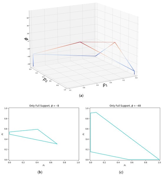
Figure 2. Visualization of the full support safe space for a $3\times 3$ game (panel (a)). Each horizontal slice of the shape is the polyhedron corresponding to the safe space given by the threshold $\varphi$, where a colder color represents a lower threshold. Panels (b) and (c) are examples of horizontal slices at thresholds $\varphi =-8$ and $\varphi =-48$, respectively. Vertices of the polyhedra vary linearly and converge to maximin strategies (typically unique, but not unique in general) at the maximin value.

Figure 3. Visualization of the overall safe space for a $3\times 3$ game (panel (a)). This shape is a union of convex subsets (though the union is not convex in general) for all sub-games obtained by using all possible supports. Panels (b) and (c) are examples of horizontal slices at $\varphi =-8$ and $\varphi =-48$, respectively. The supports are differentiated by color. One can see that the safe space is convex for one support, but the unions of safe spaces for all supports are not convex in general.

Given a payoff matrix $\mathit{A}$, our results are generated in the following way. First, we compute the column maximin value of the row payoff matrix. Since the vector of fitnesses for each player type are convex combinations of the columns of the row payoff matrix where the coefficients are the frequencies of each player type. We are looking for the maximum possible value of the minimum entry in the fitness vector under all possible convex column combinations. This is exactly the column maximin value. This maximin value is the maximum threshold given that a full-support safe space exists. Note that the maximin value may vary if the support is changed due to the irreversibility in truncation selection. Following this, we generate a set of thresholds to observe, ranging from the minimum of the payoff matrix to its maximum. When a threshold is less than or equal to the minimum, no culling happens, and when greater than the maximin value, no non-empty safe space exists for full support with respect to the maximin value.

3. Discussion

We have applied the concept of safe spaces, linear programming, and polyhedral representation conversion to two subjects of game theory: partially malicious players and independent truncation selection. Our aim was to develop methods that allow players to manage worst-case scenarios numerically.

Regarding partially malicious players, we constructed a simple model for players who are partially malicious. Such players only become malicious after securing a specified minimum payoff. If we require defensive plays against such players, we may use a generalized maximin procedure. In the case where both players have set their risk thresholds sufficiently low, both will have non-empty safe strategy sets, and thus the game could be formulated as a bilinear game (Garg et al., 2011). Future studies could develop and refine our decision rule, and the impetus for maliciousness could be directly modeled, such as by including relational utility. Additionally, truncation selection and the generalized maximin methods presented here may be used to address problems in control theory (Li et al., 2024; Liu & Zhu, 2023).

With respect to truncation selection, we showed that the equilibria are convex subsets of the probability space for each support. As the selection threshold varies linearly, the vertices of safe spaces also change linearly. When the threshold is exactly equal to the maximin value, the safe space converges to the set of maximin strategies. When the threshold is above the maximin value, extinction happens, and the game is irreversibly reduced. In general, the states do not converge to one of the Nash equilibria of the underlying game. These findings hold under the assumption of large populations, though prior work has shown how small populations can exhibit unexpected behaviors (D. B. Fogel et al., 1997; G. B. Fogel et al., 1998; G. B. Fogel & Fogel, 2011). Using the polyhedral conversion approach, we can compute the set of safe spaces analytically or less computationally intensively (with respect to the population size) than with stochastic simulations. Additionally, these methods are simpler than analyzing differential algebraic equations, which have been used to model truncation selection (Morsky & Bauch, 2016). However, our methods can still be computationally expensive for strategy spaces of high dimension. The computational complexity of polyhedral conversion algorithms depends on several factors (Bremner et al., 2009; Fukuda & Prodon, 1995): size of intermediate polytopes (sensitive to the ordering of half-spaces), dimension, number of half-spaces, and vertices. And, there exists a class of polytopes for which the double description method is exponential (Bremner et al., 2009). Nonetheless, we recommend the methods stated above for practical problems of relatively low dimension, while conducting simulations may be more practical for games of high dimension.

More broadly, our paper provides two additional scenarios in game theory requiring dense computations that benefit from linear programming and polyhedral conversion. This reinforces the value of expressing game-theoretic concepts in linear algebraic language and converting problems into feasible problems that these algorithms can solve.

4. Materials and Methods

4.1. Risk Aversion and Partially Malicious Players

We begin by defining some basic game-theoretic concepts in linear algebraic terms, since this is a useful formulation for linear and polyhedron conversion problems (which are detailed in Appendix A and Appendix B). A finite two-player normal-form game can be represented by a payoff table where the rows and columns represent the players’ pure strategies, and each entry contains a tuple of payoffs to the row and column players, respectively. For example:

$$\begin{array}{ccccc}& & L& R& \\ \begin{array}{c}U\\ D\end{array}& [& \begin{array}{c}(a_{\mathrm{row}},a_{\mathrm{col}})\\ (c_{\mathrm{row}},c_{\mathrm{col}})\end{array}& \begin{array}{c}(b_{\mathrm{row}},b_{\mathrm{col}})\\ (d_{\mathrm{row}},d_{\mathrm{col}})\end{array}& ]\end{array}.$$

(9)

We separate this table into two matrices: the row payoff matrix $\mathit{A}$, containing the first entries of each tuple; and the column payoff matrix $\mathit{B}$, containing the second entries. A mixed strategy for the row (column) player is a probability vector whose dimension equals the number of rows (columns) of the payoff table. If the row player adopts strategy $\mathit{p}$, her possible payoffs against a pure strategy playing column player is the portfolio $\mathit{a}=\left({\mathit{A}}^T\right)\mathit{p}$. Similarly, if the column player adopts strategy $\mathit{q}$, her portfolio is $\mathit{b}=\mathit{B}\mathit{q}$.

Players generally aim to maximize their payoffs, typically assuming that their opponents are rational. When this assumption fails (e.g., when opponents behave maliciously), a player’s degree of risk aversion becomes a key factor in strategy selection. Risk aversion can be measured in a variety of ways (Meyer & Meyer, 2006; Pratt, 1964). Here, we measure the risk aversion of a player’s strategy when facing an opponent whose behavior cannot be trusted to be fully rational in the following way. Consider a column player who is unsure of the rationality of their opponent (or indeed if they are malicious). The worst payoff to this player over all possible outcomes is $min\left(\mathit{B}\right)$. Let $v_{\mathrm{col}}$ denote their maximin value—their highest guaranteed payoff against any opponent. When $v_{\mathrm{col}}>min\left(\mathit{B}\right)$, we define the column player’s risk aversion for employing strategy $\mathit{q}$ as follows:

$$r_{\mathrm{col}}(\mathit{b},\mathit{B})={\displaystyle \frac{min\left(\mathit{b}\right)-min\left(\mathit{B}\right)}{v_{\mathrm{col}}-min\left(\mathit{B}\right)}},$$

(10)

where $\mathit{b}$ is the portfolio for strategy $\mathit{q}$. This equation maps $\mathit{b}$ to a real value, rescaling the payoff of the portfolio between the worst-case payoff ($r_{\mathrm{col}}=0$) and the maximin guarantee ($r_{\mathrm{col}}=1$) with intermediate values corresponding to partial risk aversion. We characterize a player by specifying a threshold value of her risk aversion ${\theta }_{\mathrm{col}}$, where she will restrict herself to strategies with risk aversion that meet or exceed it. Note that this measure is meaningful only when $min\left(\mathit{B}\right)<v_{\mathrm{col}}$, since no improvement over the worst outcome is possible otherwise.

For our model of partially malicious behavior, the objective of a partially malicious player is twofold. They prioritize obtaining a payoff that satisfies their basic needs, a minimum value they require. Once that payoff is secured, they act maliciously by minimizing their opponent’s payoff. We proceed by assuming that the column player is partially malicious. Such a player’s decision-making can be determined by the following function that takes both players’ payoffs along with a specified minimum payoff threshold and maps them to a value:

$$U({\pi }_{\mathrm{row}},{\pi }_{\mathrm{col}},{\varphi }_{\mathrm{col}})=\left\{\begin{array}{c}-\infty ,\mathrm{if}{\pi }_{\mathrm{col}}<{\varphi }_{\mathrm{col}},\hfill \\ g\left({\pi }_{\mathrm{row}}\right),\mathrm{if}{\pi }_{\mathrm{col}}\ge {\varphi }_{\mathrm{col}}.\hfill \end{array}\right.$$

(11)

${\varphi }_{\mathrm{col}}$ is the minimum payoff the column player is satisfied with, and ${\pi }_{\mathrm{row}}$ and ${\pi }_{\mathrm{col}}$ are the payoffs of the row and column player, respectively. The function $g\left(\pi \right)$ is strictly decreasing in ${\pi }_{\mathrm{row}}$, ensuring malicious behavior. For simplicity, we set $g\left(\pi \right)=-\pi$. We emphasize that, although this resembles a typical utility function, it does not satisfy the continuity axiom of expected utility maximization (John von Neumann, 1944). The negative infinity simply reflects the player’s priority of achieving the minimum required payoff before optimizing their malicious objective. In practice, a sufficiently low real value, smaller than the minimum value of g in the game, can be used to maintain consistency with the framework of expected utility.

4.2. Truncation Selection

Independent truncation selection models the evolution of the state of a population with a mixture of players who play pure strategies of a symmetric game (Morsky & Bauch, 2016). The population state $\mathit{x}$ is a vector whose entries are the proportions of the population of each strategy. The evolutionary process begins by specifying a selection pressure, a fixed threshold payoff for survival. Players compete against one another, earning payoffs from each encounter with an opponent. This process can be implemented by simulating round-robin tournaments with stochastic payoffs (D. B. Fogel et al., 1997; G. B. Fogel & Fogel, 2011), which generates a distribution of the payoffs averaged over the competitions. Payoffs may also be represented by distributions and studied with continuous dynamical systems (Morsky & Bauch, 2016). Regardless of how payoffs are particularly earned, at the end of the competition, players with averaged payoffs below the threshold are culled and do not reproduce. The remaining players each reproduce at the same rate so as to replace the culled players. In this way, players need to only have adequate payoffs that meet the threshold and receive no further benefit for exceeding it.

Our model of truncation selection assumes a large number of interactions between players. Thus, the payoff variance is negligible, and players effectively earn their fitnesses (i.e., their payoffs averaged over all interactions), the entries of the row payoff matrix $\mathit{A}$ (see Appendix C for further details). In our agent-based simulations, we initialize a population of N players of randomly determined pure strategies. In each round of the game, players earn the average payoff from each interaction and those with payoffs below the threshold $\varphi$ are culled. The remaining population reproduces to maintain the population size, rounding to the nearest whole number. This evolution is iterated until equilibria or extinction. Note that one round may be all that is required to reach an equilibrium.

Approaching this problem analytically, note that if the culling threshold payoff $\varphi$ is less than or equal to the column maximin value of $\mathit{A}$, then there exists a set of states where all player types meet or exceed the threshold. Thus, the population remains unchanged, and thus we treat such states as equilibria. We call the set of such equilibria the safe space. The set of equilibria for a given support typically forms a convex subset of the strategy simplex, and the overall safe space is the union of safe spaces for each support (note that the union of equilibria across supports is not convex in general). Assuming a full-support state (for other supports, one simply crosses out the corresponding rows and columns that are not in support), we can compute these equilibria via the following polyhedral conversion problem:

$$\begin{array}{c}\hfill \mathrm{convert}\mathrm{from}\mathrm{H}-\mathrm{to}\mathrm{V}-\mathrm{representation}:\\ \hfill 1={\mathbf{1}}^T\mathit{x}\\ \hfill \mathbf{0}\le \mathit{I}\mathit{x}\\ \hfill \varphi \mathbf{1}\le \mathit{A}\mathit{x}\end{array}$$

(12)

The first two constraints restrict the solution space inside the probability simplex, while the last enforces the equilibrium condition (i.e., that the payoffs of all player-types meet or exceed $\varphi$).

When $\varphi$ is less than or equal to the column maximin value of $\mathit{A}$, the vertices in V-representation form a convex subset of the probability simplex. When the $\varphi$ is exactly the column maximin value of $\mathit{A}$, the V-representation is exactly the set of maximin strategies (typically single points, but can be a convex set in general). When $\varphi$ is above the column maximin value of $\mathit{A}$, the polyhedron is the empty set. Thus, all states will have at least one player type go extinct, reducing the game to a sub-game. States outside of a non-empty safe space may evolve toward this space, toward a reduced game, or toward complete extinction of all player types.

References

- Avis, D., & Fukuda, K. (1991, June 10–12). A pivoting algorithm for convex hulls and vertex enumeration of arrangements and polyhedra. Seventh Annual Symposium on Computational Geometry (pp. 98–104), North Conway, NH, USA. [Google Scholar]
- Avis, D., Fukuda, K., & Picozzi, S. (2002). On canonical representations of convex polyhedra. In Mathematical software (pp. 350–360). World Scientific. [Google Scholar]
- Binmore, K. (1992). Fun and games. In A text on game theory. D. C. Heath & Co. [Google Scholar]
- Bremner, D., Sikiric, M. D., & Schürmann, A. (2009). Polyhedral representation conversion up to symmetries. In CRM proceedings (Vol. 48, pp. 45–72). Springer. [Google Scholar]
- Bruyere, V., Filiot, E., Randour, M., & Raskin, J.-F. (2014, April 5–6). Expectations or guarantees? I want it all! A crossroad between games and MDPs. 2nd International Workshop on Strategic Reasoning (Vol. 146, pp. 1–8), Grenoble, France. [Google Scholar]
- Burton-Chellew, M. N., El Mouden, C., & West, S. A. (2016). Conditional cooperation and confusion in public-goods experiments. Proceedings of the National Academy of Sciences of the United States of America, 113(5), 1291–1296. [Google Scholar] [CrossRef] [PubMed]
- Cressman, R., & Tao, Y. (2014). The replicator equation and other game dynamics. Proceedings of the National Academy of Sciences of the United States of America, 111(Suppl. 3), 10810–10817. [Google Scholar] [CrossRef]
- Dave, A., & Malikopoulos, A. A. (2024). Approximate information states for worst case control and learning in uncertain systems. IEEE Transactions on Automatic Control, 70(1), 127–142. [Google Scholar] [CrossRef]
- Dickhaut, J., & Kaplan, T. (1993). A program for finding Nash equilibria. In Economic and financial modeling with mathematica® (pp. 148–166). Springer. [Google Scholar] [CrossRef]
- Etessami, K., & Yannakakis, M. (2010). On the complexity of Nash equilibria and other fixed points. SIAM Journal on Computing, 39(6), 2531–2597. [Google Scholar] [CrossRef]
- Ficici, S. G. (2006, July 8–12). A game-theoretic investigation of selection methods in two-population coevolution. 8th Annual Conference on Genetic and Evolutionary Computation (pp. 321–328), Seattle, WA, USA. [Google Scholar] [CrossRef]
- Ficici, S. G., Melnik, O., & Pollack, J. B. (2005). A game-theoretic and dynamical-systems analysis of selection methods in coevolution. IEEE Transactions on Evolutionary Computation, 9(6), 580–602. [Google Scholar] [CrossRef]
- Ficici, S. G., & Pollack, J. B. (2000, July 10–12). Effects of finite populations on evolutionary stable strategies. 2nd Annual Conference on Genetic and Evolutionary Computation (pp. 927–934), Las Vegas, NV, USA. [Google Scholar]
- Ficici, S. G., & Pollack, J. B. (2007). Evolutionary dynamics of finite populations in games with polymorphic fitness equilibria. Journal of Theoretical Biology, 247(3), 426–441. [Google Scholar] [CrossRef]
- Fogel, D. B., Fogel, G. B., & Andrews, P. C. (1997). On the instability of evolutionary stable strategies. BioSystems, 44(2), 135–152. [Google Scholar] [CrossRef]
- Fogel, G. B., Andrews, P. C., & Fogel, D. B. (1998). On the instability of evolutionary stable strategies in small populations. Ecological Modelling, 109(3), 283–294. [Google Scholar] [CrossRef]
- Fogel, G. B., & Fogel, D. B. (2011). Simulating natural selection as a culling mechanism on finite populations with the hawk–dove game. BioSystems, 104(1), 57–62. [Google Scholar] [CrossRef] [PubMed]
- Fudenberg, D., & Liang, A. (2019). Predicting and understanding initial play. American Economic Review, 109(12), 4112–4141. [Google Scholar] [CrossRef]
- Fukuda, K., & Prodon, A. (1995). Double description method revisited. In Franco-Japanese and Franco-Chinese conference on combinatorics and computer science (pp. 91–111). Springer. [Google Scholar]
- Ganzfried, S. (2023, December 13–15). Safe equilibrium. 2023 62nd IEEE Conference on Decision and Control (CDC) (pp. 5230–5236), Singapore. [Google Scholar]
- Garg, J., Jiang, A. X., & Mehta, R. (2011). Bilinear games: Polynomial time algorithms for rank based subclasses. In International workshop on internet and network economics (pp. 399–407). Springer. [Google Scholar]
- Harsanyi, J. C. (1968). Games with incomplete information played by ‘bayesian’ players. Management Science. [Google Scholar]
- Henrich, J., McElreath, R., Barr, A., Ensminger, J., Barrett, C., Bolyanatz, A., Cardenas, J. C., Gurven, M., Gwako, E., & Henrich, N. (2006). Costly punishment across human societies. Science, 312(5781), 1767–1770. [Google Scholar] [CrossRef] [PubMed]
- Holler, M. J. (1990). The unprofitability of mixed-strategy equilibria in two-person games: A second folk-theorem. Economics Letters, 32(4), 319–323. [Google Scholar] [CrossRef]
- Holler, M. J. (1992). Nash equilibrium reconsidered and an option for maximin. Quality and Quantity, 26(3), 323–335. [Google Scholar] [CrossRef]
- Holler, M. J., & Høst, V. (2019). Maximin vs. Nash equilibrium: Theoretical results and empirical evidence. In Optimal decisions in markets and planned economies (pp. 245–255). Routledge. [Google Scholar]
- Htun, Y. (2005). Irrationality in game theory. World Scientific. [Google Scholar]
- Jebari, K., & Madiafi, M. (2013). Selection methods for genetic algorithms. International Journal of Emerging Sciences, 3(4), 333–344. [Google Scholar]
- John von Neumann, O. M. (1944). Theory of games and economic behavior. Princeton University Press. [Google Scholar]
- Li, J., Yang, M., Lewis, F. L., & Zheng, M. (2024). Compensator-based self-learning: Optimal operational control for two-time-scale systems with input constraints. IEEE Transactions on Industrial Informatics, 20(7), 9465–9475. [Google Scholar] [CrossRef]
- Liu, Y., & Zhu, Q. (2023). Event-triggered adaptive neural network control for stochastic nonlinear systems with state constraints and time-varying delays. IEEE Transactions on Neural Networks and Learning Systems, 34(4), 1932–1944. [Google Scholar] [CrossRef]
- Lucchetti, R. (2006). Linear programming and game theory. In Convexity and well-posed problems (pp. 117–137). Springer. [Google Scholar]
- Meyer, D., & Meyer, J. (2006). Measuring risk aversion. Foundations and Trends in Microeconomics, 2, 107–203. [Google Scholar] [CrossRef]
- Morsky, B., & Bauch, C. T. (2016). Truncation selection and payoff distributions applied to the replicator equation. Journal of Theoretical Biology, 404, 383–390. [Google Scholar] [CrossRef]
- Morsky, B., & Bauch, C. T. (2019). The impact of truncation selection and diffusion on cooperation in spatial games. Journal of Theoretical Biology, 466, 64–83. [Google Scholar] [CrossRef]
- Morsky, B., Smolla, M., & Akçay, E. (2020). Evolution of contribution timing in public goods games. Proceedings of the Royal Society B, 287(1927), 20200735. [Google Scholar] [CrossRef]
- Moscibroda, T., Schmid, S., & Wattenhofer, R. (2009). The price of malice: A game-theoretic framework for malicious behavior. Internet Mathematics, 6(2), 125–156. [Google Scholar] [CrossRef]
- Myerson, R. B. (1991). Game theory: Analysis of conflict. Harvard University Press. [Google Scholar]
- Nash, J. F. (1950). Equilibrium points in n-person games. Proceedings of the National Academy of Science of the United States of America, 36(1), 48–49. [Google Scholar] [CrossRef] [PubMed]
- Papadimitriou, C. H. (2007). The complexity of finding Nash equilibria. Algorithmic Game Theory, 2, 30. [Google Scholar]
- Parrilo, P. A. (2006, December 13–15). Polynomial games and sum of squares optimization. 45th IEEE Conference on Decision and Control (pp. 2855–2860), San Diego, CA, USA. [Google Scholar] [CrossRef]
- Porter, R., Nudelman, E., & Shoham, Y. (2008). Simple search methods for finding a Nash equilibrium. Games and Economic Behavior, 63(2), 642–662. [Google Scholar] [CrossRef]
- Pratt, J. W. (1964). Risk aversion in the small and in the large. Econometrica, 32(1/2), 122–136. [Google Scholar] [CrossRef]
- Selten, R., & Bielefeld, R. S. (1988). Examination of the perfectness concept for equilibrium points in extensive games. In Models of strategic rationality (Vol. 2). Theory and Decision Library C. Springer. [Google Scholar]
- Simon, H. A. (1955). A behavioral model of rational choice. The Quarterly Journal of Economics, 69, 99–118. [Google Scholar] [CrossRef]
- Simons, S. (1995). Minimax theorems and their proofs. In Minimax and applications (pp. 1–23). Springer. [Google Scholar]
- Su, R., & Morsky, B. (2024). Relational utility and social norms in games. Mathematical Social Sciences, 127, 54–61. [Google Scholar] [CrossRef]
- Thie, P. R., & Keough, G. E. (2011). An introduction to linear programming and game theory. John Wiley & Sons. [Google Scholar]
- Von Stengel, B. (2021). Game theory basics. Cambridge University Press. [Google Scholar]
- Wright, J., & Leyton-Brown, K. (2014, June 8–12). Level-0 meta-models for predicting human behavior in games. EC 2014—Proceedings of the 15th ACM Conference on Economics and Computation, Palo Alto, CA, USA. [Google Scholar] [CrossRef]
Disclaimer/Publisher’s Note: The statements, opinions and data contained in all publications are solely those of the individual author(s) and contributor(s) and not of MDPI and/or the editor(s). MDPI and/or the editor(s) disclaim responsibility for any injury to people or property resulting from any ideas, methods, instructions or products referred to in the content. |
© 2025 by the authors. Licensee MDPI, Basel, Switzerland. This article is an open access article distributed under the terms and conditions of the Creative Commons Attribution (CC BY) license (https://creativecommons.org/licenses/by/4.0/).