An Efficient Decoder for the Recognition of Event-Related Potentials in High-Density MEG Recordings ^†

Abstract

Brain–computer interfacing (BCI) is a promising technique for regaining communication and control in severely paralyzed people. Many BCI implementations are based on the recognition of task-specific event-related potentials (ERP) such as P300 responses. However, because of the high signal-to-noise ratio in noninvasive brain recordings, reliable detection of single trial ERPs is challenging. Furthermore, the relevant signal is often heterogeneously distributed over several channels. In this paper, we introduce a new approach for recognizing a sequence of attended events from multi-channel brain recordings. The framework utilizes spatial filtering to reduce both noise and signal space considerably. We introduce different models that can be used to construct the spatial filter and evaluate the approach using magnetoencephalography (MEG) data involving P300 responses, recorded during a BCI experiment. Compared to the accuracy achieved in the BCI experiment performed without spatial filtering, the recognition rate increased significantly to up to 95.3% on average (SD: 5.3%). In combination with the data-driven spatial filter construction we introduce here, our framework represents a powerful method to reliably recognize a sequence of brain potentials from high-density electrophysiological data, which could greatly improve the control of BCIs.

1. Introduction

People who have lost the capability to communicate with their environment due to severe paralysis could greatly benefit from a brain–computer interface (BCI) [1]. In such systems, communication can be realized by translating voluntarily modulated brain activity of a user into commands. One type of brain signal used for BCI-based communication is the event-related potential (ERP), which is evoked in response to specific external events. A prominent ERP, often focused on in BCI research, is the P300 potential, which is elicited in oddball paradigms by rare deviant target stimuli, randomly embedded in a series of frequent standard stimuli. Because the P300 is a marker of focused attention, it is used in BCIs to infer where the users direct their attention. With the so-called matrix speller this approach was introduced in 1988 [2] and has been widely used ever since. In ERP detection, the main challenge researchers are faced with is the low signal-to-noise ratio (SNR), which is due to ongoing brain activity, artifacts, and environmental noise. Consequently, the detection of ERPs in single time intervals is challenging. However, the SNR of ERP components increases when averaging the brain responses to several identical events. Thus, pooling of many ERP intervals increases the recognition success, but leads to a low information transfer rate (ITR). Furthermore, noninvasive electrophysiological measurement techniques indirectly measure effects of local source activity, resulting in heterogeneously distributed signals across several channels. An appropriate combination of these channels enhances the signal strength and reduces the noise. Such channel weightings are also known as spatial filter coefficients which were applied to analyze P300 potentials, taking varying approaches to estimating the coefficients, e.g., independent component analysis (ICA) [3], common spatial patterns (CSP) [4], spatial whitening [5], canonical correlation analysis (CCA) [6], and others [7,8]. A quite simple example of a spatial filter is averaging the signal across all channels, weighting all channels equally. However, if channels represent the subcomponents differently or are completely uninvolved, this approach is disadvantageous. Therefore, when a high number of channels is available and no hypothetical selection of channels can be made, optimal spatial filtering is particularly relevant.

In general, noninvasive BCIs are implemented using electroencephalographic (EEG) measurements. In a previous study, we investigated magnetoencephalographic (MEG) recordings as an alternative acquisition modality for use in a BCI, providing a high number of sensors with short preparation time of subjects. The study [9] aimed at virtual object selection combined with robotic grasping. MEG is regarded as having exquisite spatial and temporal resolution [1]. In previous work [10], we demonstrated greater discrimination of adjacent motor potentials in MEG data compared with simultaneously recorded EEG data. Furthermore, a study investigating the classification of visual ERPs [11] has provided evidence that discriminable data are more focused in the MEG than in the EEG. The potential advantages of MEG could open a promising communication channel for severely impaired patients, even though only applicable in a laboratory environment. In this work, we apply new methods to the previously recorded 248 channel MEG data for an improved decoding of the P300 responses. In contrast to the empirically parameterized decoding scheme we used in the MEG-based BCI performed without spatial filtering, our new approach is data-driven and does not need a priori assumptions regarding spatial patterns or, in a particular variant, regarding the time course.

In this paper we introduce a new method to efficiently recognize distinct sequences of event related potentials. The approach does not use machine learning techniques for classification but determines the target sequence by means of the Pearson product-moment correlation coefficient. The framework is specifically designed to work with CCA. We demonstrate the outcome of the recognition approach using different model functions that take event-specific information into account. In contrast to CSP, which estimates spatial filters considering events separately as well, here also temporal characteristics can be involved. Importantly, we introduce a simple model that determines the waveform of most discriminative ERP components and permits accurate recognition of the target event sequence.

2. Materials and Methods

In this section, we propose a new method that projects high-density electrophysiological data into a subspace consisting of a few virtual channels using CCA. Furthermore, we describe a simple approach to recognizing sequences of ERPs from these virtual channels, which is essential in many BCI applications. The proposed method is specifically suited to ERP processing, since the model assumes time-locked brain responses. Thus, synchronously driven BCIs could greatly benefit from this approach when applying dense electrode configurations.

This section is organized as follows. First we introduce the CCA method, which is the mathematical tool we apply to estimate filter matrices. Subsequently, we explain our approach of constructing the reference signal. Then we define several models for reference signals, which are used to construct spatial and temporal filters with CCA. In the following subsection, we describe how the filter matrices can be applied to perform an efficient recognition of ERP sequences. Afterwards, we present the experimental data we used for evaluation of the algorithm. Finally, we describe the processing steps we applied to perform the evaluation. In the Appendix we provide the nomenclature describing all symbols used in this section.

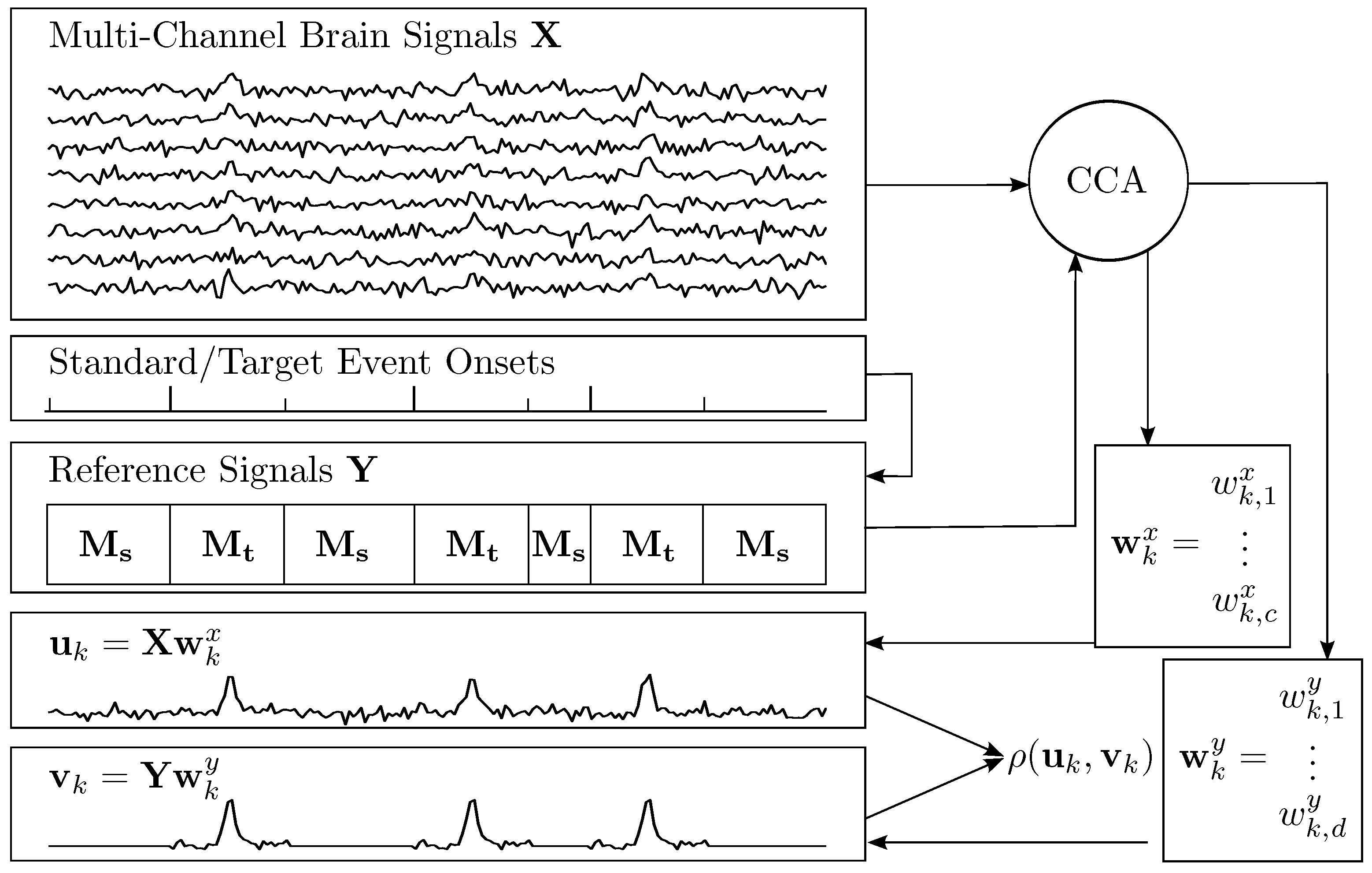
2.1. Canonical Correlation Analysis

A basic concept in our approach is the transformation of multi-channel data such that relevant information is extracted while noise and redundancy is reduced. To achieve this, we apply canonical correlation analysis, an established multivariate statistical method, which was first introduced by Hotelling [12]. The rationale behind CCA is the transformation of two sets of variables, such that the values of the transformed variable sets show high similarity. Considering two sets $\mathbf{X}\in {\mathbb{R}}^{n\times c}$ and $\mathbf{Y}\in {\mathbb{R}}^{n\times d}$ of c and d variables ($c\ge d$) and n observations, CCA finds the maximum correlation of linear combinations of the columns in $\mathbf{X}$ and $\mathbf{Y}$. The linear combinations $\mathbf{U}=\mathbf{X}{\mathbf{W}}_x,{\mathbf{W}}_x\in {\mathbb{R}}^{c\times d}$ and $\mathbf{V}=\mathbf{Y}{\mathbf{W}}_y,{\mathbf{W}}_y\in {\mathbb{R}}^{d\times d}$ that have maximum correlation are called canonical variables. Thus, the problem to be solved is to find the matrices ${\mathbf{W}}_x$ and ${\mathbf{W}}_y$ such that the kth canonical correlation ${\rho }_k({\mathbf{u}}_k,{\mathbf{v}}_k),k=1,\dots ,d$ is maximal, given that ${\mathbf{u}}_k$ and ${\mathbf{v}}_k$ are centred:

$$\underset{{\mathbf{w}}_k^x,{\mathbf{w}}_k^y}{\text{max}}{\rho }_k({\mathbf{u}}_k,{\mathbf{v}}_k)=\frac{E\left({\mathbf{u}}_k^T{\mathbf{v}}_k\right)}{\sqrt{E\left({\mathbf{u}}_k^T{\mathbf{u}}_k\right)E\left({\mathbf{v}}_k^T{\mathbf{v}}_k\right)}}.$$

(1)

An important property of the canonical variables is that they are uncorrelated amongst themselves. Analogously to principal component analysis (PCA), where successive variance maximization reveals orthogonal factors, the first canonical variable reveals the linear combination that achieves maximum correlation, while the following canonical variables maximize the correlation of residual variance in the data. Thus, a number of at most d canonical variables can be transformed, while the canonical correlation ${\rho }_k$ decreases with increasing k. The equivalent relationship of $\rho (\mathbf{u},\mathbf{v})=\rho (\mathbf{v},\mathbf{u})$ implies that it is irrelevant whether the number of variables is higher in $\mathbf{X}$ or in $\mathbf{Y}$.

While CCA operates on two different sets of variables, other transformation algorithms like PCA and ICA operate on a single set of variables. Other algorithms such as the CSP method operate on two sets of identical variables containing different observations. It was shown in sensorimotor rhythm-based studies that the categorical information involved in this approach is advantageous for spatial filtering [13]. However, temporal information which is important for ERP analysis is not regarded with ordinary CSP [4]. The concept of CCA enables the modeling of an independent set of variables serving as reference signals [14,15]. Thus, CCA can be used to exploit categorical and temporal information to estimate efficient spatio-temporal filters for BCI control.

2.2. Constructing Spatial Filters for ERP Extraction

Let us assume the set of variables $\mathbf{X}$ is represented by a number of c channels and n sampling points of a time-varying signal, measuring brain activity. To find a spatial filter that decomposes a component that maximally correlates with an ERP, we need to know the waveform of the brain response. This requires a priori knowledge, which is not necessarily available. As mentioned above, CCA determines a linear combination $\mathbf{X}{\mathbf{W}}_x$ and $\mathbf{Y}{\mathbf{W}}_y$ with maximum correlation. Thus, it can be applied to linearly combine a set of d signals in $\mathbf{Y}$ that yield the characteristic signal $\mathbf{Y}{\mathbf{w}}_k^y$ with maximum correlation to $\mathbf{X}{\mathbf{w}}_k^x$. To obtain the spatial filter matrix ${\mathbf{W}}_x$ using CCA, we need to model a set of reference signals $\mathbf{Y}$, characterizing a hypothetical brain response to the onsets of specific events. Here we consider a sequence of two types of events: target events and standard events. Consequently, we define a set of d model ERPs ${\mathbf{M}}_{\mathbf{t}}\in {\mathbb{R}}^{\mathbf{n}\times \mathbf{d}}$ describing a target event and ${\mathbf{M}}_{\mathbf{s}}\in {\mathbb{R}}^{\mathbf{n}\times \mathbf{d}}$ describing the model ERP of a standard event, where n is the number of sampling points in the ERP interval. We construct the reference functions $\mathbf{Y}$ that are associated with a sequence of standard and target events by embedding an arbitrary model ${\mathbf{M}}_{\mathbf{s}}$ at each onset $i_s$ of the standard event in chronological order, i.e.,

$$y_{i+i_s,k}=m_{(i,k)}^s,i=1,\dots ,n,k=1,\dots ,d.$$

(2)

Afterwards, we embed an arbitrary model ${\mathbf{M}}_{\mathbf{t}}$ at each onset $i_t$ of the target event analogous to Equation (2):

$$y_{i+i_t,k}=m_{(i,k)}^t,i=1,\dots ,n,k=1,\dots ,d.$$

(3)

When n is greater than the distance between two events, the previously assigned values in $\mathbf{Y}$ are overwritten. See Figure 1 for an illustration of the analysis method. Note that all signals depicted in the figure are actually represented as column vectors, and that the estimation of only one component is shown.

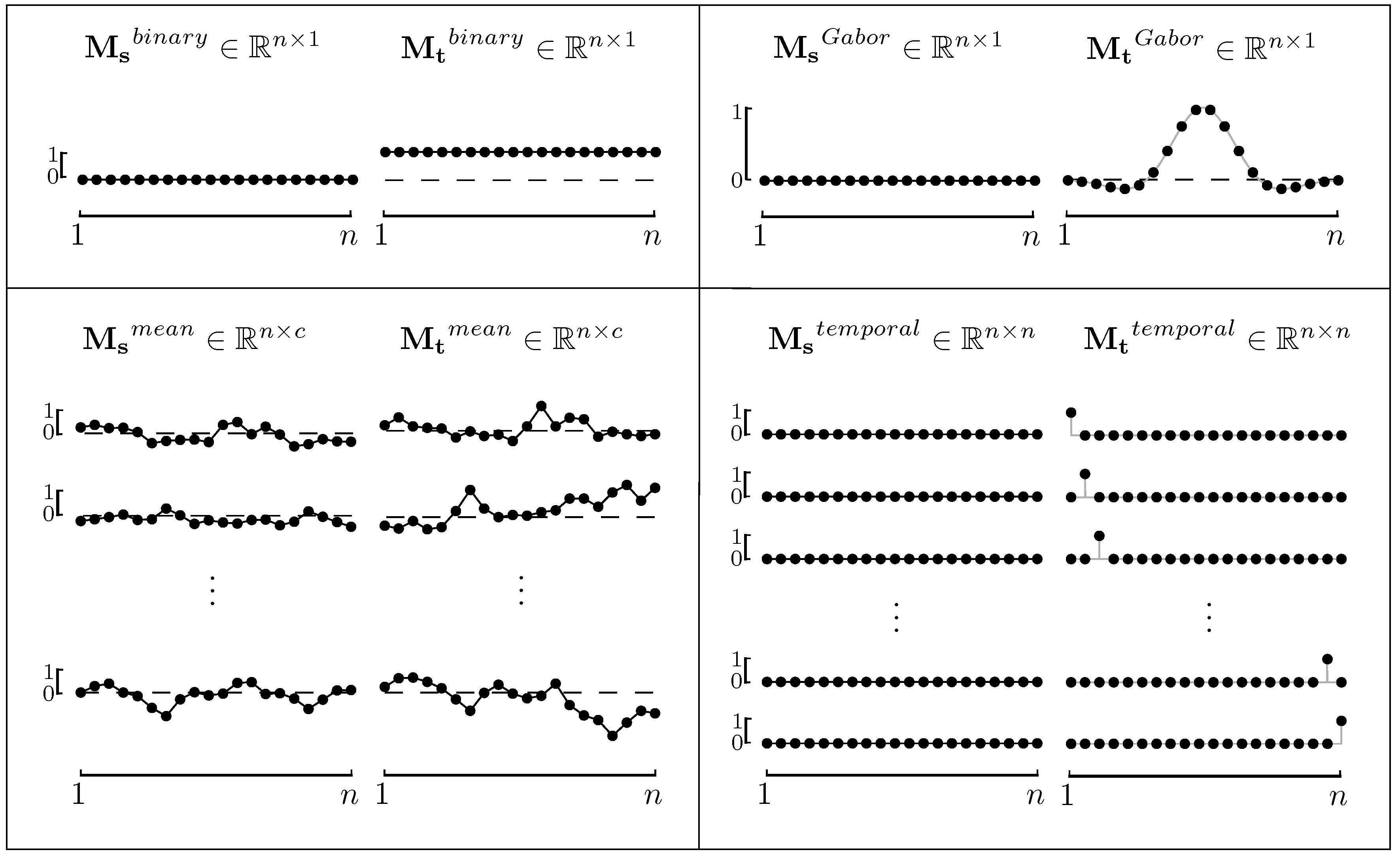
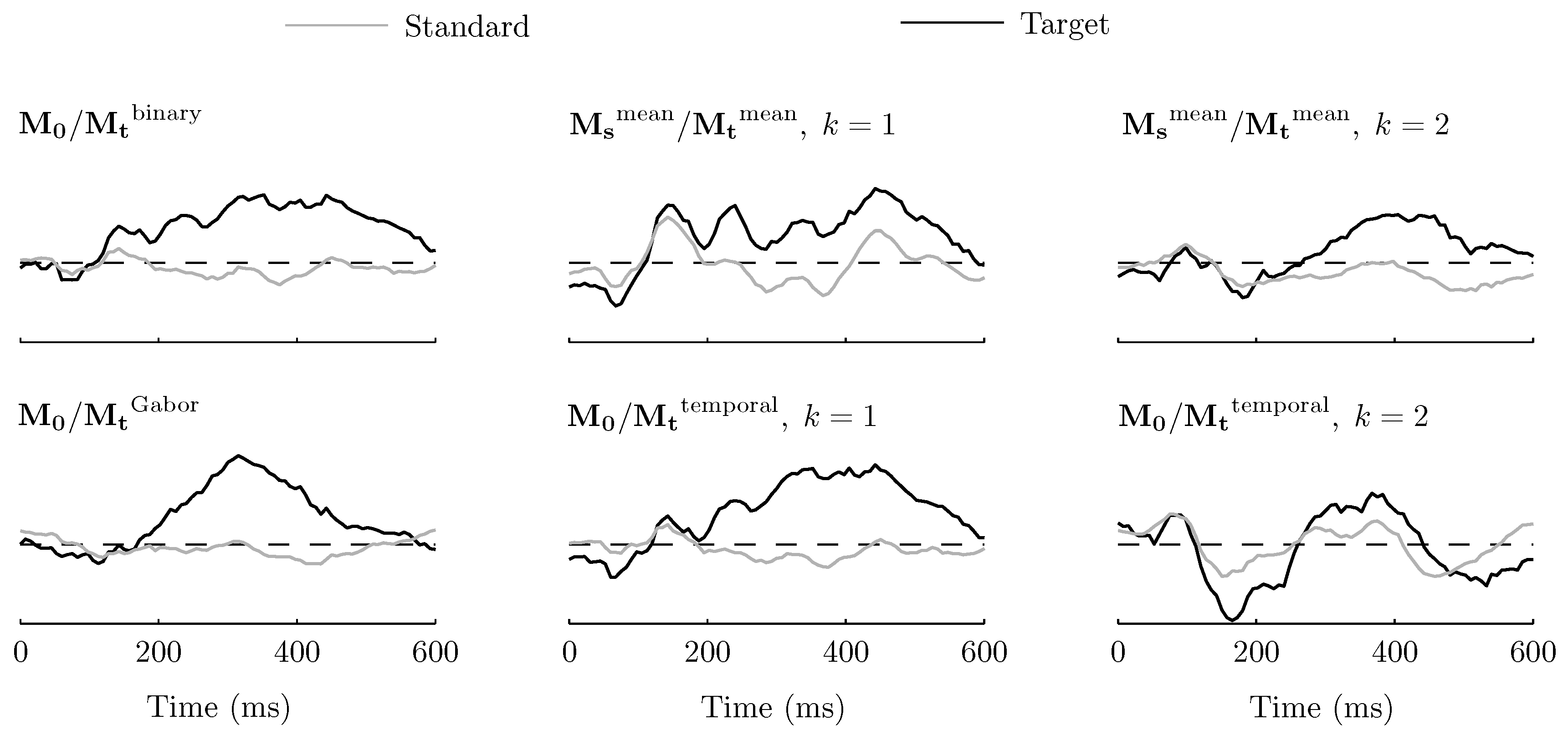
2.3. Model Functions for ERPs

The functions we will define in this section aim at characterizing ERPs, i.e., they represent assumptions about the expected brain response following a specific event. First we describe two simple model functions that we consider to be applicable in decoding ERPs following a target event. The most general hypothesis is that the brain response is deflected during the interval of the target event but not when standard events are presented. We can model this hypothesis by defining binary model functions of length n as follows:

$${{\mathbf{M}}_{\mathbf{s}}}^{\text{binary}}=\left(m_{i,1}\right),\text{where}{m}_{i,1}=\left\{0|\forall i=1,\dots ,n\right\}$$

(4)

$${{\mathbf{M}}_{\mathbf{t}}}^{\text{binary}}=\left(m_{i,1}\right),\text{where}{m}_{i,1}=\left\{1|\forall i=1,\dots ,n\right\}.$$

(5)

The assumption that no characteristic deflection is expected after standard events will be made several times in this paper, which is why we also will refer to the zero matrix ${\mathbf{M}}_{\mathbf{0}}$ if ${\mathbf{M}}_{\mathbf{s}}$ is all zero. Certainly, the binary model reflects a quite naïve assumption, because we know that brain responses do not switch on and off but respond to events with bell-shaped deflections. In single trial analysis, typical ERP responses were shown to fit with Gabor functions [16]. Thus, to model a single ERP deflection, we define for the target event interval:

$${{\mathbf{M}}_{\mathbf{t}}}^{\text{Gabor}}=\left(m_{i,1}\right),\text{where}{m}_{i,1}={\mathrm{e}}^{-\frac{{(i-\mu )}^2}{2{\sigma }^2}}cos\frac{2\pi (i-\mu )}{\omega \sigma }.$$

(6)

In this equation μ denotes the sample point of the signal peak, σ represents the standard deviation of the Gaussian component in samples and ω is a scaling parameter where $\omega \sigma$ spans one cosine cycle.

So far we have solely described single reference functions, which simplifies CCA to multiple correlation analysis. However, to exploit the strength of CCA, we intend to model a set of multiple distinct reference functions. One approach was introduced by Spüler et al. [6], who calculated the average signal across all standard trials as ${{\mathbf{M}}_{\mathbf{s}}}^{\text{mean}}\in {\mathbb{R}}^{n\times c}$ and across all target trials in a set of training data as ${{\mathbf{M}}_{\mathbf{t}}}^{\text{mean}}\in {\mathbb{R}}^{n\times c}$, where c is the number of channels to be involved. The advantage of this method is that the reference functions are directly calculated from the brain data representing one time course for each channel with reduced noise. Thus, this method is less driven by hypothesis but rather the underlying brain response is determined in a data-driven manner.

2.4. A Spatio-Temporal Filter

The approach of averaging over trials still has one restricting assumption, which is the time course of the signal within single channels. The weights of the vector ${\mathbf{w}}_k^y$ in ${\mathbf{W}}_y$ determine the contribution of the averaged signal in channel $i,i=1,\dots ,c$ to the kth ERP component. Thus, internally two spatial filter matrices are determined with CCA, one for the input signal and one for the averaged signal. Another point to be noted is that due to the broad spatial distribution of ERP activity many of the channels representing average signals over trials might reflect similar signals, implying redundancy in the reference functions. To resolve this constraint, we introduce a set of reference functions which is orthogonal and which models the time course of the signal rather than the composition of predefined signal courses. We define ${{\mathbf{M}}_{\mathbf{t}}}^{\text{temporal}}$ as d signal time series, where each of the time series represents one sample point after the event of interest occurred, and d is the number of samples the interval of interest is spanning. More specifically, we define

$${{\mathbf{M}}_{\mathbf{t}}}^{\text{temporal}}={\mathbf{I}}_d$$

(7)

where ${\mathbf{I}}_d$ is the identity matrix of size d. Consequently, the d coefficients in ${\mathbf{w}}_k^y$ determine the strength at sample point $i,i=1,\dots ,d$ after event onset. This model can also be seen as a set of impulse functions where each function $i,i=1,\dots ,d$ shows exactly one peak at time point i. In combination with ${\mathbf{M}}_{\mathbf{0}}$ the weights in ${\mathbf{w}}_k^y$ directly represent the estimated signal in the interval of interest that distinguish event-related brain activity from baseline activity. Here, each vector ${\mathbf{w}}_k^y$ in ${\mathbf{W}}_y$ can be considered a temporal filter. As already explained above, using CCA, the filter matrix ${\mathbf{W}}_x$ simultaneously weights the c channels such that the correlation with the estimated temporally filtered reference signal is maximal. This linear weighting of channels is a classical spatial filter. The time series ${\mathbf{u}}_k$ obtained from spatial filtering can be considered a virtual channel. An important feature of our approach is that the evoked potential is determined implicitly by the method applied. To make this clear, consider the virtual channel ${\mathbf{v}}_k=\mathbf{Y}{\mathbf{w}}_k^y$. Setting $\mathbf{Y}={\mathbf{I}}_d$ implies that ${\mathbf{w}}_k^y={\mathbf{v}}_k$, which means that the filter ${\mathbf{w}}_k^y$ directly represents the estimated component ${\mathbf{v}}_k$, maximal correlating with ${\mathbf{u}}_k$, i.e., with the channel signals filtered by ${\mathbf{w}}_k^x$. Consequently, when using this filter we obtain $\mathbf{V}={\mathbf{M}}_{\mathbf{0}}{\mathbf{W}}_y=\mathbf{0}$ for standard events and $\mathbf{V}={{\mathbf{M}}_{\mathbf{t}}}^{temporal}{\mathbf{W}}_y={\mathbf{W}}_y$ for target events, meaning that the filtered channel signals $\mathbf{U}$ are supposed to correlate with a zero signal after standard events and to correlate with the spatial filter coefficients in ${\mathbf{W}}_y$ after target events. Because each column in $\mathbf{Y}$ represents a model function which in turn represents a time point after stimulus onset in chronological order, the elements in ${\mathbf{w}}_k^y$ can be considered the time course of virtual channel k. Using this spatio-temporal filter the only hypothetical assumption is that a characteristic signal is evoked after a specific event occurred, and no systematic activity is otherwise present. This represents an even more data-driven approach as compared to using ${{\mathbf{M}}_{\mathbf{s}}}^{\text{mean}}$ and ${{\mathbf{M}}_{\mathbf{t}}}^{\text{mean}}$ as models. Note that the reliable estimation of filters ${\mathbf{W}}_x$ and ${\mathbf{W}}_y$ using CCA requires a multitude of repetitions of the same events, irrespective of the model functions we have introduced. More precisely, in every model function ${\mathbf{y}}_k$ the value $m_{i,k}$ of time point i after event onset has to be present many times to enhance the signal-to-noise ratio. Thus, although ${\mathbf{M}}_{\mathbf{s}}$ and ${\mathbf{M}}_{\mathbf{t}}$ are repeatedly represented in a sequence of events (Equation (2) and Equation (3)), multiple such sequences must be involved simultaneously in the CCA to enhance the reliability of estimated ERP components.

2.5. Recognition of ERP Sequences

Many BCIs are controlled by P300 responses, elicited by attention to one of several stimuli. In such systems, the selection of an item is determined by recognizing which of the item-specific event sequences match the brain response best. Generally, this is done by pooling the single responses to an item stimulus. Here we use the Pearson product-moment correlation coefficient to evaluate the similarity of measured and expected sequences of ERPs. An event sequence codes an item uniquely. In the CCA based filter construction method described above, a set of ERP waveforms with maximum correlation with the measured data is determined using the canonical coefficients ${\mathbf{W}}_y$. Simultaneously, the corresponding spatial filter ${\mathbf{W}}_x$ extracts the noise reduced signal components. Thus, we determine ${\mathbf{W}}_x$ from a set of training data that we subsequently apply to new data as a spatial filter. For this purpose, we concatenate the measured brain signals from all trials in $\mathbf{X}\in {\mathbb{R}}^{n\times c}$ where n is the total number of sample points and c is the number of channels. Furthermore, we concatenate the corresponding set of reference functions $\mathbf{Y}\in {\mathbb{R}}^{n\times d}$. We then use these sets of variables to perform the CCA according to Equation (1). This reveals d virtual channels and d canonical variables, respectively. According to the Matlab implementation of CCA [17], the significance level $p_k$ for canonical variable k is determined using a ${\chi }^2$ statistic for the null hypothesis that all ${\rho }_i,i=k,\dots ,d$ are zeros. For further processing, we reduce the number of components, and consequently the number of filters to be applied on test data by selecting only the first q filters that provide a significance of $p_k<0.05$ where at the same time the canonical correlation obtained from training data have to exceed a value of ${\rho }_k>0.1$. Thus, after estimating the filters from training data we obtain a spatial filter ${\mathbf{W}}_x\in {\mathbb{R}}^{c\times q}$ for the brain data, and another filter ${\mathbf{W}}_y\in {\mathbb{R}}^{d\times q}$ for the reference data.

To recognize an ERP sequence from new brain signal recordings $\widehat{\mathbf{X}}$, a model ${\widehat{\mathbf{Y}}}_e$ is generated for each of the events, assuming event e is the target event. Afterwards, for each model, the correlations ${\rho }_{k,e}$ are determined as

$${\rho }_{k,e}=\frac{E({\widehat{\mathbf{u}}}_k^T{\widehat{\mathbf{v}}}_{k,e})}{\sqrt{E({\widehat{\mathbf{u}}}_k^T{\widehat{\mathbf{u}}}_k)E({\widehat{\mathbf{v}}}_{k,e}^T{\widehat{\mathbf{v}}}_{k,e})}},$$

(8)

where ${\widehat{\mathbf{u}}}_k=\widehat{\mathbf{X}}{\mathbf{w}}_k^x$ and ${\widehat{\mathbf{v}}}_{k,e}={\widehat{\mathbf{Y}}}_{\mathbf{e}}{\mathbf{w}}_k^y$. The correlations are then transformed using Fisher’s z-transform and averaged over the canonical variables:

$$f\left(e\right)=\frac{1}{q}\sum _{k=1}^q\frac{1}{2}ln(\frac{1+{\rho }_{k,e}}{1-{\rho }_{k,e}}).$$

(9)

The model providing the highest average correlation with the spatially filtered brain data is then assumed to represent the target event:

$$\underset{e}{\text{argmax}}f\left(e\right).$$

(10)

In Figure 2, we demonstrate the recognition procedure showing an exemplary trial, where the ERP sequence was correctly recognized. In this example, the fourth sequence provides the highest correlation between ${\widehat{\mathbf{v}}}_{1,4}$ and ${\widehat{\mathbf{u}}}_1$, indicated by blue coloring. Note that we show only the first canonical variable, although the classification result might also be affected by other canonical variables.

2.6. Experimental Data

The data set previously described in [9] consists of recordings from 17 subjects. MEG data at 248 head coil positions and 23 reference coils were measured and digitized at 678.15 Hz. During the experiment, subjects performed an oddball task involving selecting one of six virtual objects by covert attention to object-related visual stimuli. The objects were arranged around a fixation cross, on which the subjects fixated during each trial. Visual stimulation was performed by flashing a marker for each object for 100 ms, with inter-stimulus intervals of 300 ms in random order. The subject directed his/her attention to the flash of the target object, which served as the deviant stimulus, and ignored all other flashes representing standard stimuli of an oddball task. In one trial, each object marker was flashed five times, resulting in 30 stimuli within 9 s. To avoid an overlap of attention-related brain activity, we accounted for a minimum latency of 600 ms between flashes of a single object in the randomization procedure. Subjects performed six to eight runs of instructed selection, as well as additional runs, in which they freely selected the objects. One run consisted of 18 trials. Only those runs in which selections were instructed are involved in this study, providing the subject’s true intention for decoder training and evaluation. For more details on the experiment please refer to [9].

2.7. Processing of Experimental Data

In a first step, the MEG data were segmented into epochs of 10 s, starting at the first flash event of a trial. Subsequently, the DC offset was removed, and noise cancellation was performed by removing environmental noise captured from reference sensors according to Robinson [18]. This step effectively removes slow signal drifts in the MEG. Thus, no spectral filtering is required for our analysis method. We performed the analysis using the original sampling rate but also repeated the analysis using down-sampled data with decimation factors 2, 5, 10 and 20 (339.08 Hz, 135.63 Hz, 67.82 Hz and 33.91 Hz). The first two runs were used to estimate the spatial filter matrix ${\mathbf{W}}_x$ , concatenating all trials to form the matrices $\mathbf{X}$ and $\mathbf{Y}$. The remaining runs served as test data to evaluate the performance of the approach. We defined the interval size of an expected ERP at 600 ms. We tested our algorithm using the model ERPs ${\mathbf{M}}_{\mathbf{0}}$/${{\mathbf{M}}_{\mathbf{t}}}^{\text{binary}}$, ${\mathbf{M}}_{\mathbf{0}}$/${{\mathbf{M}}_{\mathbf{t}}}^{\text{Gabor}}$ (μ and σ were set to accord with 300 ms and 100 ms, $\omega =5$), ${{\mathbf{M}}_{\mathbf{s}}}^{\text{mean}}$/${{\mathbf{M}}_{\mathbf{t}}}^{\text{mean}}$, and ${\mathbf{M}}_{\mathbf{0}}$/${{\mathbf{M}}_{\mathbf{t}}}^{\text{temporal}}$. Please see Figure 3 for a visualization of the model functions. In this figure exemplary data for $n=20$ samples are shown. Note that $c=248$ and that the horizontally presented time series are actually column vectors.

3. Results

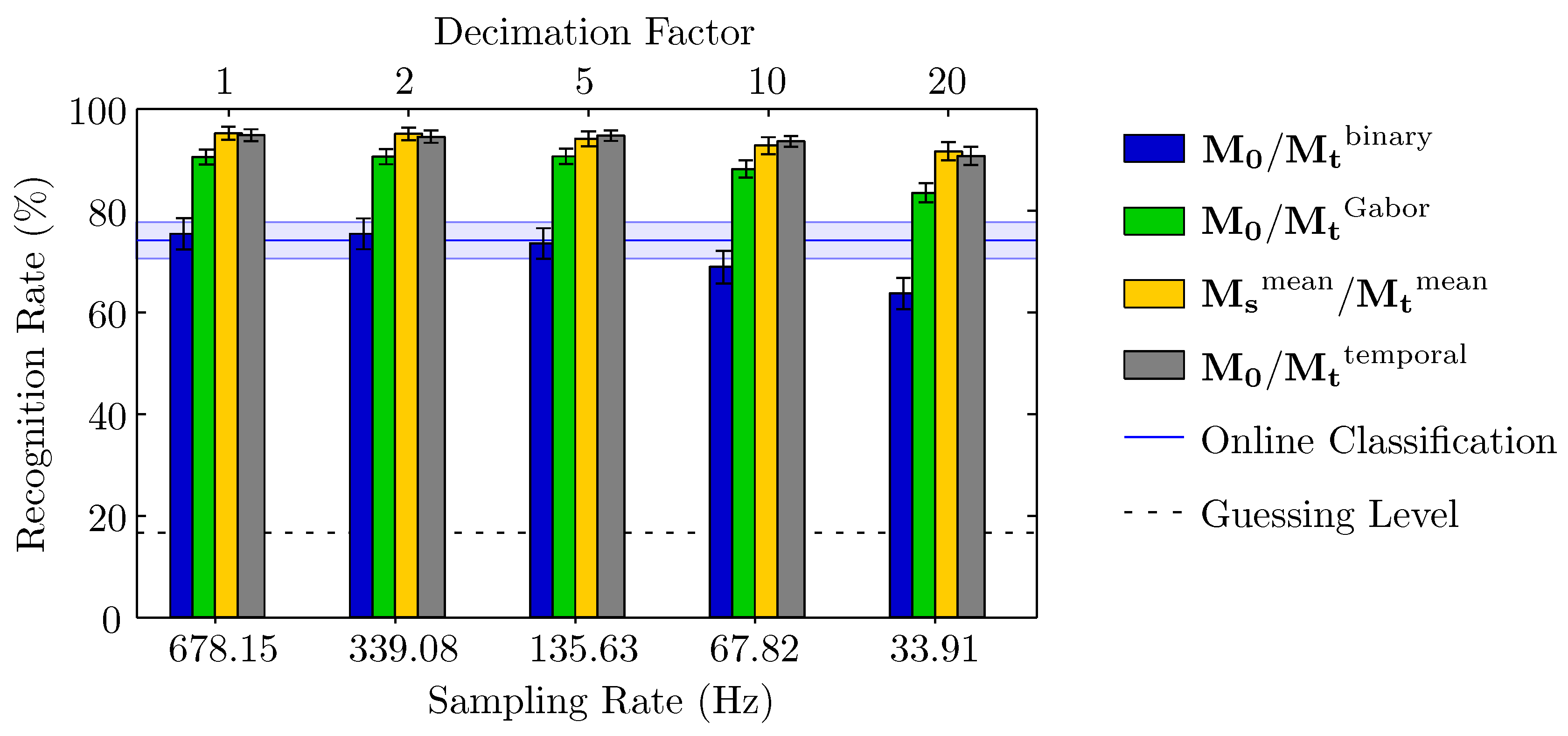
3.1. Accuracy of Recognition

With our recognition algorithm, we were able to significantly improve the accuracy using the model ERPs ${\mathbf{M}}_{\mathbf{0}}$/${{\mathbf{M}}_{\mathbf{t}}}^{\text{Gabor}}$, ${{\mathbf{M}}_{\mathbf{s}}}^{\text{mean}}$/${{\mathbf{M}}_{\mathbf{t}}}^{\text{mean}}$, and ${\mathbf{M}}_{\mathbf{0}}$/${{\mathbf{M}}_{\mathbf{t}}}^{\text{temporal}}$ (see Figure 4). In the actual experiment, feedback was presented according to a support vector machine (SVM) classification. The algorithm applied in [9] selected 64 sensors out of 152 hypothetically pre-selected sensors for classification. Data were filtered between 1 Hz and 12 Hz and re-sampled to 32 Hz. For instructed selections, this approach provided a recognition rate of 74.1% on average (SD: 14.8%). Applying our new approach the highest recognition rates were achieved without down-sampling and using model function sets ${\mathbf{M}}_{\mathbf{0}}$/${{\mathbf{M}}_{\mathbf{t}}}^{\text{mean}}$ (mean: 95.3%, SD: 5.3%) and ${\mathbf{M}}_{\mathbf{0}}$/${{\mathbf{M}}_{\mathbf{t}}}^{\text{temporal}}$ (mean: 94.9%, SD: 4.8%). Twelve subjects achieved a recognition rate of more than 95%, which corresponds to an ITR of more than 13.1 bit/min, given the choice of 6 alternatives within 10 s. This is substantially higher than the average ITR of 6.9 bit/min achieved with the initial decoding approach. Reducing the sampling rate and consequently also the computational effort for performing CCA (

Table 1. Computational effort using different model functions and applying different sampling rates. The mean effort and standard deviation denote the time in seconds which is needed to perform the CCA on the training set using an Intel Xeon CPU E5649.

Decimation Factor	${\mathbf{M}}_{\mathbf{0}}$/${{\mathbf{M}}_{\mathbf{t}}}^{\mathbf{binary}}$	${\mathbf{M}}_{\mathbf{0}}$/${{\mathbf{M}}_{\mathbf{t}}}^{\mathbf{Gabor}}$	${{\mathbf{M}}_{\mathbf{s}}}^{\mathbf{mean}}$/${{\mathbf{M}}_{\mathbf{t}}}^{\mathbf{mean}}$	${\mathbf{M}}_{\mathbf{0}}$/${{\mathbf{M}}_{\mathbf{t}}}^{\mathbf{temporal}}$
1	16.09 (1.23)	16.10 (1.29)	33.95 (2.70)	48.80 (3.87)
2	8.33 (1.01)	8.23 (0.97)	17.97 (3.14)	15.52 (1.39)
5	3.05 (0.29)	3.19 (0.49)	6.46 (0.58)	3.93 (0.33)
10	1.41 (0.13)	1.41 (0.16)	2.93 (0.27)	1.53 (0.16)
20	0.61 (0.14)	0.63 (0.11)	1.27 (0.15)	0.64 (0.11)

), the recognition rate was almost constant up to a sampling rate of 67.82 Hz and only slightly reduced to 91.8% and 90.8%, respectively, when using a decimation factor of 20. Both models, ${\mathbf{M}}_{\mathbf{0}}$/${{\mathbf{M}}_{\mathbf{t}}}^{\text{mean}}$ and ${\mathbf{M}}_{\mathbf{0}}$/${{\mathbf{M}}_{\mathbf{t}}}^{\text{temporal}}$ obviously were suited similarly for the recognition task, revealing accuracies that are nonsignificantly different. The much simpler model ${\mathbf{M}}_{\mathbf{0}}$/${{\mathbf{M}}_{\mathbf{t}}}^{\text{Gabor}}$ also considerably outperformed our initial classification approach, achieving recognition rates of more than 90.5% (SD: 6.3%) at sampling rates above 135 Hz and slightly reduced accuracy using lower sampling rates. Remarkably, the simplest model ${\mathbf{M}}_{\mathbf{0}}$/${{\mathbf{M}}_{\mathbf{t}}}^{\text{binary}}$ achieved comparable recognition rates as compared to the initial online classification, using sampling rates above 135 Hz, but accuracy decreased at lower sampling rates. An important advantage of our spatial filter approach was that the number of channels could be considerably reduced from 248 channels to a few components (

Table 2. Number of selected components using different model functions and applying different sampling rates. The values denote mean and standard deviation.

Decimation Factor	${\mathbf{M}}_{\mathbf{0}}$/${{\mathbf{M}}_{\mathbf{t}}}^{\mathbf{binary}}$	${\mathbf{M}}_{\mathbf{0}}$/${{\mathbf{M}}_{\mathbf{t}}}^{\mathbf{Gabor}}$	${{\mathbf{M}}_{\mathbf{s}}}^{\mathbf{mean}}$/${{\mathbf{M}}_{\mathbf{t}}}^{\mathbf{mean}}$	${\mathbf{M}}_{\mathbf{0}}$/${{\mathbf{M}}_{\mathbf{t}}}^{\mathbf{temporal}}$
1	1.0 (0.0)	1.0 (0.0)	13.6 (1.2)	5.0 (0.8)
2	1.0 (0.0)	1.0 (0.0)	14.8 (1.2)	5.1 (0.8)
5	1.0 (0.0)	1.0 (0.0)	7.7 (1.2)	4.9 (0.8)
10	1.0 (0.0)	1.0 (0.0)	7.6 (1.3)	4.8 (1.0)
20	1.0 (0.0)	1.0 (0.0)	7.3 (1.4)	4.6 (1.1)

), where each virtual channel was composed of one of the selected spatial filters. Note that the number of selected components shown in Table 2 corresponds to the q most significant canonical correlations we determined as described in Section 2.5. The number of components, available after CCA is given by $min\left\{c,d\right\}$ and thus depends on the number of channels $c=248$ and the size of the set of model functions d. For the single model functions ${\mathbf{M}}_{\mathbf{0}}$/${{\mathbf{M}}_{\mathbf{t}}}^{\text{binary}}$ and ${\mathbf{M}}_{\mathbf{0}}$/${{\mathbf{M}}_{\mathbf{t}}}^{\text{Gabor}}$ is $d=1$, for ${\mathbf{M}}_{\mathbf{0}}$/${{\mathbf{M}}_{\mathbf{t}}}^{\text{mean}}$ is $d=248$ and for ${\mathbf{M}}_{\mathbf{0}}$/${{\mathbf{M}}_{\mathbf{t}}}^{\text{temporal}}$ d depends on the interval length and sampling rate, resulting in $d\in \left\{407,203,81,41,20\right\}$ for decimation factors 1, 2, 5, 10 and 20. Furthermore, the recognition method summarizes the waveform of each virtual channel as one single feature, directly describing the similarity of the measured waveform to the expected waveform. Thus, a substantial reduction of the feature set can be achieved, down to a single feature using single model ERPs. Finally, no multivariate classification technique was required to determine the attended stimulus, but rather the feature directly determined the most probable event sequence.

To demonstrate the resulting filtered signal achieved with different model function sets, we show averages of the virtual channels across standard and target intervals for a representative subject in Figure 5.

In order to further emphasize the advantage of the recognition framework combined with CCA-estimated filter matrices we also performed an ordinary classification approach and determined the impact of PCA as an alternative spatial filtering method. We used the same analysis interval as we used with model functions at 33.91 Hz sampling rate, no spectral filtering and SVM-based selection of 64 channels out of the whole channel set to train an SVM and test the classifier with the validation framework described above. This approach is a trade-off between the decoder used in the actual BCI experiment and the new approach by loosening the hypothetical constraints which were spectral filtering and pre-selecting sensors. This revealed an average recognition rate of 81.1% (SD: 13.8%). When performing a PCA prior to classification and using the 64 virtual channels representing highest variance, the recognition rate was at a comparable level (mean: 82.4%, SD: 12.4%). This is significantly higher than the accuracy achieved in the online experiment, but neither the PCA outperforms SVM classification of spatially unfiltered data nor accuracies at the level achieved with the proposed recognition approach could be achieved.

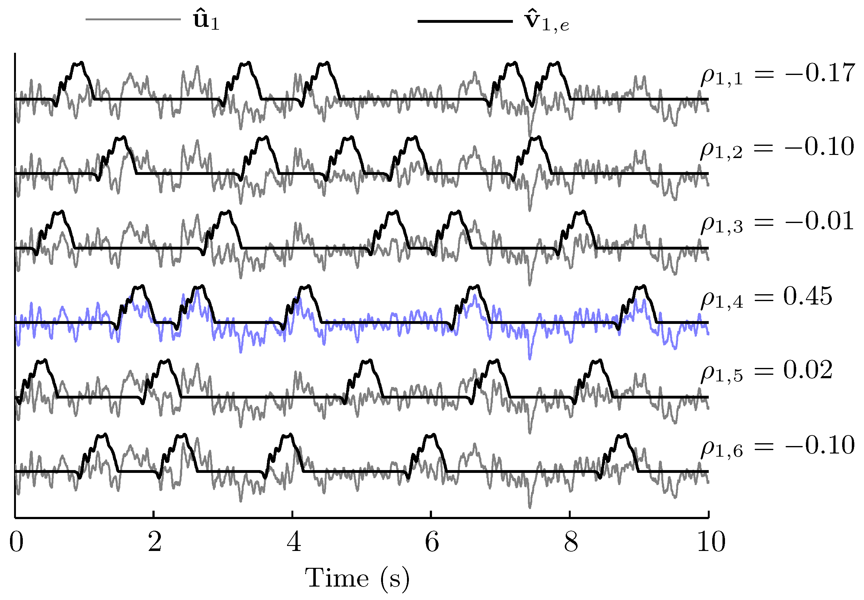
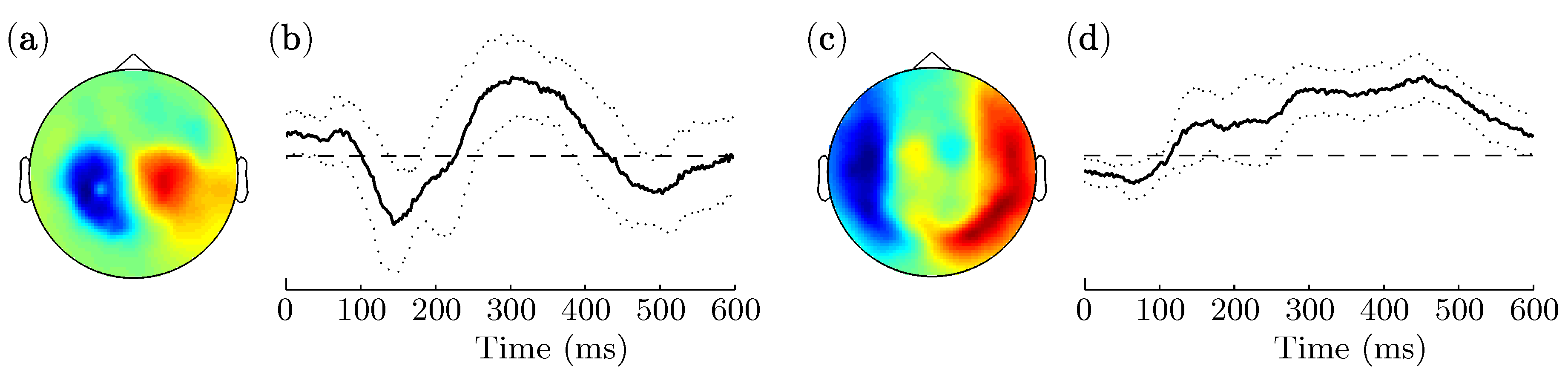
3.2. Spatio-Temporal Patterns

In the Methods section, we mentioned the benefit of using the model ${\mathbf{M}}_{\mathbf{0}}$/${{\mathbf{M}}_{\mathbf{t}}}^{\text{temporal}}$, specifically the opportunity to obtain the time course of ERP subcomponents from a data-driven linear transformation of the input signals. Here we evaluate the outcome of using this specific model function in combination with CCA. Note that the data filtered by CCA-estimated matrices, which we denote ERP subcomponents that are reflected in virtual channels, do not correspond to physiological sources according to the theory of blind source separation [19]. Rather, they also are mixtures of brain sources, but in contrast to the linear combinations of brain sources obtained in the original sensor space they are optimized to represent the brain’s response to a target event.

The virtual channels obtained for each subject varied in terms of spatial distribution, waveform, and significance ranking. Even though individual brain patterns revealed individual spatio-temporal filters, there were two typical spatio-temporal patterns that could be observed in most of the subjects, where at least one of the two patterns was present in every subject. In Figure 6, we show the estimated waveforms of these two components as an average over subjects (standard deviation is indicated by dotted lines). The waveform corresponds to the target event intervals in ${\mathbf{v}}_k$, which is with ${{\mathbf{M}}_{\mathbf{t}}}^{\text{temporal}}$ by definition identical to ${\mathbf{w}}_k^y$. The topographic maps show the loadings calculated as the correlation between ${\mathbf{x}}_i,i=1,\dots ,c$ and ${\mathbf{v}}_k$, averaged over subjects. This measure is comparable to the factor loadings known from PCA. Red areas indicate positive correlation of the sensor signals with the extracted waveform, blue areas indicate negative correlations. Thus, the waveforms shown in Figure 6 correlate with the magnetic flux measured over the right hemisphere, and the reversed curves correlate with the magnetic flux measured over the left hemisphere. Similar patterns showing ingoing magnetic field lines over the right and outgoing magnetic field lines over the left hemisphere were also found in [20]. One typical waveform we observed in 12 subjects, appeared over parietal areas and peaked at approximately 300 ms, which is an expected component in an oddball paradigm. The component also showed a negative undershoot before and after the positive gain. The canonical correlation of this component was ${\rho }_k=0.27$ on average (SD: 0.05) and was ranked three times as the strongest canonical correlation, six times as the 2nd, and three times as the 3rd component. Another prominent waveform was found in 14 of the subjects and extended over a long interval between 100 and 600 ms. This slow wave can also be found in EEG data that investigate deviant stimuli and has a posterior-positive, anterior-negative scalp distribution [21]. This is in line with the bilateral distribution of magnetic fluctuations shown in Figure 6. In the MEG, this component appears to have a higher impact than the classical P300, because this component was ranked in nine subjects as the first and four times as the second component, and achieved an average canonical correlation of ${\rho }_k=0.32$ (SD: 0.05). It is important to note that additionally to these two striking components, other individual components were also extracted, which are difficult to interpret but contributed to a reliable recognition of an event sequence.

4. Discussion

Our results show that our new approach facilitates the recognition of ERP sequences with a high accuracy. A core component of our method is the optimal spatial filtering, which projects high-density MEG data into a subspace of a few components. Depending on the complexity of the ERP model used as reference signal, a high number of channels can be reduced to only one virtual channel, providing highly reliable recognition rates. The highest accuracies were achieved equally with two different sets of model functions. The first set was based on empirical estimates constructing reference signals according to [6] and the second set was designed to compose the temporal evolution of the signal. Using the latter method, CCA constructs a spatial filter matrix and concurrently determines brain dynamics. Thus, using CCA combined with appropriate reference functions, we can interpret the filtered signal as ERP components that represent the task-specific brain activity. Importantly, the final recognition of the target sequence is based on the statistical correlation measure and does not require machine learning algorithms. Simulating a real BCI application, we used only two runs to estimate the filter matrices for subsequent ERP prediction, resulting in a training time for each subject of less than ten minutes. Our recognition method showed significantly higher recognition rates than the decoding approach without spatial filtering applied in [9] for three of the proposed sets of reference functions modeling the ERPs. Using MEG , our method efficiently deals with high sampling rates and therefore does not require spectral filtering and down-sampling. In contrast, down-sampled data does not provide advantage in terms of accuracy. Rather, a sampling rate between 20 and 40 Hz, as typically used in P300 detection algorithms using EEG [5,6,22,23], yielded slightly lower recognition rates compared with sampling the data at higher rates.

Given the uncommon setup of our experiment for object selection, comparison with other studies is challenging. BCI systems are often compared in terms of the information transfer rate. However, the ITR depends on accuracy, the number of selectable items and the duration of the entire selection process. When decoding accuracy is used as evaluation measure, it must be considered in the context of the guessing level, which depends on the number of selectable items. P300 detection from noninvasive recordings is a common application in BCI matrix spellers, where 36 symbols are usually provided. In such BCI systems, average bandwidths of 20 to 30 bit/min were achieved at acceptable accuracy levels (> 85%) with advanced decoding techniques [3,8,24,25]. It is important to note that the inter-stimulus interval, the number of stimuli and the number of selectable items used in the MEG experiment limits the maximum ITR to 15.5 bit/min, if detection was hundred percent. However, when we use the symbol rate as evaluation measure, our classification procedure led to an average of 5.7 symbols/min at 95.1% decoding accuracy, exceeding the performance of previously described matrix spellers [3,8,24]. In a study largely fitting our experimental parameters, several classifiers, electrode configurations and trial lengths were investigated using a 6-item oddball task [23]. The highest achieved classification accuracy at a trial length of approximately 10 s was about 93% on average, which is slightly less than the accuracy achieved using our approach.

One of the sets of model functions we introduced, the set that models temporal characteristics, renders the CCA-based estimation of optimal spatial filters a method to estimate a spatio-temporal filter. Because we made a minimum of hypothetical assumptions with this model, the method is highly data-driven. The resulting optimally filtered brain signals can be interpreted as an optimal combination of ERP subcomponents, which are produced individually for each user and which can be applied to identify the target ERP sequence. Although some components are unique and difficult to interpret, we identified two components that showed a characteristic waveform and spatial distribution across most of the subjects. Interestingly, a slow wave component was more prominent than the component peaking at 300 ms. In an MEG study on P300 source activity [20], peaks were found between 400 and 600 ms showing comparable time courses as the slow wave component found in the present study. The patterns showing highest correlation between this component and the magnetic flux we found laterally in temporal sensors. In the BCI experiment we initially performed when the data were recorded, the recognition rate was significantly lower than with the new approach. Presumably, this was the case because we excluded sensors located over the temporal lobe empirically from this initial decoding approach due to assumptions derived from EEG experiments. A further hypothetical processing step in the initial approach was applying a band-pass filter with passband 1 Hz to 12 Hz, which is common in EEG based BCIs [23] but probably canceled out the slow wave component. This is also supported by the fact that classification without spectral filtering and without excluding sensors was superior compared to the online results. However, even performing PCA as an alternative approach to reduce the number of channels could not reveal recognition accuracies as high as it has been achieved with CCA-based recognition, which also accords to findings from classifying ERPs in a workload task [26]. This demonstrates the advantage of our data-driven approach compared with a hypothesis-driven approach and the capability of CCA to efficiently extract task-related features.

So far, in the field of processing electrophysiological data optimization of correlation was mainly used for analyzing band power in brain signals, such as extracting components that correlate with intensity modulation of auditory stimuli [27] and discovering underlying power-to-power couplings of neuronal sources [28]. Similarly, CCA was used to detect steady-state visual evoked potentials for BCI control [14,15]. The classification of ERPs obtained from CCA by building reference functions from trial averages in combination with a linear discriminant classifier was first introduced by Spüler et al. [6] and recently compared with other spatial filters [26], revealing a superior performance compared to PCA. In the present paper we adapted this approach for recognizing sequences of events by a simple correlation measure and showed that alternative model functions can be used in this framework as reference signals as well.

We have demonstrated the efficacy of our method when applied to high-density MEG data, but it is important to note that MEG has only limited suitability for BCI use. A main limitation is the mobility of the acquisition system, making applications only possible within the laboratory. Nevertheless, e.g. locked-in patients could benefit from an efficient communication, despite the limitation to laboratory dependence. The methods developed with MEG data also may help to advance EEG processing, because signal characteristics of MEG and EEG measurements are similar. Finally, MEG could serve as a training modality for demanding neurofeedback applications as it is approached in rehabilitation or ADHD treatment.

5. Conclusions

The spatial and spatio-temporal filters presented in this paper, revealed considerably higher recognition accuracy in spatially highly resolved MEG data compared to classification in the original sensor space. The supervised estimation of optimal spatial filters in combination with a correlation based recognition framework is highly advantageous compared to PCA combined with a classifier based on learning theory. We presume that the proposed methods are applicable to high-density EEG recordings as well, and that the framework can be used for other ERP recognition tasks, not being limited to the oddball paradigm. In particular, the algorithm could greatly improve BCI reliability for improved communication abilities of severely paralyzed people.

References

1. Birbaumer, N.; Cohen, L.G. Brain-computer interfaces: Communication and restoration of movement in paralysis. J. Physiol. 2007, 579, 621–636. [Google Scholar] [CrossRef] [PubMed]
2. Farwell, L.A.; Donchin, E. Talking off the top of your head: Toward a mental prosthesis utilizing event-related brain potentials. Electroencephalogr. Clin. Neurophysiol. 1988, 70, 510–523. [Google Scholar] [CrossRef]
3. Serby, H.; Yom-Tov, E.; Inbar, G.F. An improved P300-based brain-computer interface. IEEE Trans. Neural Syst. Rehabil. Eng. 2005, 13, 89–98. [Google Scholar] [CrossRef] [PubMed]
4. Krusienski, D.; Sellers, E.; Vaughan, T. Common spatio-temporal patterns for the P300 speller. In Proceedings of the CNE ’07. 3rd International IEEE/EMBS Conference on Neural Engineering, Kohala Coast, HI, USA, 2–5 May 2007; pp. 421–424.
5. Farquhar, J.; Hill, N.J. Interactions between pre-processing and classification methods for event-related-potential classification: Best-practice guidelines for brain-computer interfacing. Neuroinformatics 2013, 11, 175–192. [Google Scholar] [CrossRef] [PubMed]
6. Spüler, M.; Walter, A.; Rosenstiel, W.; Bogdan, M. Spatial filtering based on canonical correlation analysis for classification of evoked or event-related potentials in EEG data. IEEE Trans. Neural Syst. Rehabil. Eng. 2014, 22, 1097–1103. [Google Scholar] [CrossRef] [PubMed]
7. Rivet, B.; Souloumiac, A.; Attina, V.; Gibert, G. xDAWN algorithm to enhance evoked potentials: Application to brain-computer interface. IEEE Trans. Biomed. Eng. 2009, 56, 2035–2043. [Google Scholar] [CrossRef] [PubMed] [Green Version]
8. Pires, G.; Nunes, U.; Castelo-Branco, M. Statistical spatial filtering for a P300-based BCI: Tests in able-bodied, and patients with cerebral palsy and amyotrophic lateral sclerosis. J. Neurosci. Methods 2011, 195, 270–281. [Google Scholar] [CrossRef] [PubMed]
9. Reichert, C.; Kennel, M.; Kruse, R.; Heinze, H.J.; Schmucker, U.; Hinrichs, H.; Rieger, J.W. Brain-controlled selection of objects combined with autonomous robotic grasping. In Neurotechnology, Electronics, and Informatics; Springer: Cham, Switzerland, 2015; Volume 13, pp. 65–78. [Google Scholar]
10. Quandt, F.; Reichert, C.; Hinrichs, H.; Heinze, H.J.; Knight, R.T.; Rieger, J.W. Single trial discrimination of individual finger movements on one hand: A combined MEG and EEG study. Neuroimage 2012, 59, 3316–3324. [Google Scholar] [CrossRef] [PubMed]
11. Bianchi, L.; Sami, S.; Hillebrand, A.; Fawcett, I.P.; Quitadamo, L.R.; Seri, S. Which physiological components are more suitable for visual ERP based brain-computer interface? A preliminary MEG/EEG study. Brain Topogr. 2010, 23, 180–185. [Google Scholar] [CrossRef] [PubMed]
12. Hotelling, H. The most predictable criterion. J. Educ. Psychol. 1935, 26, 139–142. [Google Scholar] [CrossRef]
13. Blankertz, B.; Tomioka, R.; Lemm, S.; Kawanabe, M.; Müller, K.R. Optimizing spatial filters for robust EEG single-trial analysis. IEEE Signal Process. Mag. 2008, 25, 41–56. [Google Scholar] [CrossRef]
14. Lin, Z.; Zhang, C.; Wu, W.; Gao, X. Frequency recognition based on canonical correlation analysis for SSVEP-based BCIs. IEEE Trans. Biomed. Eng. 2006, 53, 2610–2614. [Google Scholar] [CrossRef] [PubMed]
15. Reichert, C.; Kennel, M.; Kruse, R.; Hinrichs, H.; Rieger, J.W. Efficiency of SSVEF recognition from the magnetoencephalogram—A Comparison of spectral feature classification and CCA-based prediction. In Proceedings of the International Congress on Neurotechnology, Electronics and Informatics, Algarve, Portugal, 18–20 September 2013; pp. 233–237.
16. Sielużycki, C.; König, R.; Matysiak, A.; Kuś, R.; Ircha, D.; Durka, P. Single-trial evoked brain responses modeled by multivariate matching pursuit. IEEE Trans. Biomed. Eng. 2009, 56, 74–82. [Google Scholar] [CrossRef] [PubMed]
17. Matlab implementation of CCA. Available online: www.mathworks.com/help/stats/canoncorr.html (accessed on 12 April 2016).
18. Robinson, S.E. Environmental noise cancellation for biomagnetic measurements. In Advances in Biomagnetism; Springer: New York, NY, USA, 1989; pp. 721–724. [Google Scholar]
19. Congedo, M.; Gouy-Pailler, C.; Jutten, C. On the blind source separation of human electroencephalogram by approximate joint diagonalization of second order statistics. Clin. Neurophysiol. 2008, 119, 2677–2686. [Google Scholar] [CrossRef] [PubMed]
20. Mecklinger, A.; Maess, B.; Opitz, B.; Pfeifer, E.; Cheyne, D.; Weinberg, H. A MEG analysis of the P300 in visual discrimination tasks. Electroencephalogr. Clin. Neurophysiol. 1998, 108, 45–56. [Google Scholar] [CrossRef]
21. Spencer, K.M.; Dien, J.; Donchin, E. Spatiotemporal analysis of the late ERP responses to deviant stimuli. Psychophysiology 2001, 38, 343–358. [Google Scholar] [CrossRef] [PubMed]
22. Krusienski, D.J.; Sellers, E.W.; Cabestaing, F.; Bayoudh, S.; McFarland, D.J.; Vaughan, T.M.; Wolpaw, J.R. A comparison of classification techniques for the P300 speller. J. Neural Eng. 2006, 3, 299–305. [Google Scholar] [CrossRef] [PubMed] [Green Version]
23. Hoffmann, U.; Vesin, J.M.; Ebrahimi, T.; Diserens, K. An efficient P300-based brain-computer interface for disabled subjects. J. Neurosci. Methods 2008, 167, 115–125. [Google Scholar] [CrossRef] [PubMed]
24. Donchin, E.; Spencer, K.M.; Wijesinghe, R. The mental prosthesis: Assessing the speed of a P300-based brain-computer interface. IEEE Trans. Rehabil. Eng. 2000, 8, 174–179. [Google Scholar] [CrossRef] [PubMed]
25. Lenhardt, A.; Kaper, M.; Ritter, H.J. An adaptive P300-based online brain-computer interface. IEEE Trans. Neural Syst. Rehabil. Eng. 2008, 16, 121–130. [Google Scholar] [CrossRef] [PubMed]
26. Roy, R.N.; Bonnet, S.; Charbonnier, S.; Jallon, P.; Campagne, A. A comparison of ERP spatial filtering methods for optimal mental workload estimation. In Proceedings of the 2015 37th Annual International Conference of the IEEE Engineering in Medicine and Biology Society (EMBC), Milan, Italy, 25–29 August 2015; pp. 7254–7257.
27. Dähne, S.; Meinecke, F.C.; Haufe, S.; Höhne, J.; Tangermann, M.; Müller, K.R.; Nikulin, V.V. SPoC: A novel framework for relating the amplitude of neuronal oscillations to behaviorally relevant parameters. Neuroimage 2014, 86, 111–122. [Google Scholar] [CrossRef] [PubMed]
28. Dähne, S.; Nikulin, V.V.; Ramírez, D.; Schreier, P.J.; Müller, K.R.; Haufe, S. Finding brain oscillations with power dependencies in neuroimaging data. Neuroimage 2014, 96, 334–348. [Google Scholar] [CrossRef] [PubMed]
Figure 1. Depiction of the method of estimating filter matrices for extracting event-related potential (ERP) components based on canonical correlation analysis (CCA).
Computers 05 00005 g001
Figure 2. Demonstration of ERP Recognition.
Computers 05 00005 g002
Figure 3. Model functions used to perform CCA for ERP recognition. Dots represent discrete function values at sample points in the interval of the expected ERP (600 ms, n = 20 ).
Computers 05 00005 g003
Figure 4. Recognition rates achieved with different ERP models at different sampling rates. Error bars indicate standard error of the mean.
Computers 05 00005 g004
Figure 5. Averaged, spatially filtered signal revealed with different ERP models exemplary for one subject. For multi-function models the first two components are shown.
Computers 05 00005 g005
Figure 6. Averaged loadings for (a) a parietal P300-like component and (b) the corresponding waveform; as well as (c) a potentially inferior-medial located component and (d) the corresponding waveform. Color scale of loadings in (a) and (c) as well as amplitude in (b) and (d) have arbitrary units.
Computers 05 00005 g006