Robust Feature Matching Method for SAR and Optical Images by Using Gaussian-Gamma-Shaped Bi-Windows-Based Descriptor and Geometric Constraint

Abstract

Improving the matching reliability of multi-sensor imagery is one of the most challenging issues in recent years, particularly for synthetic aperture radar (SAR) and optical images. It is difficult to deal with the noise influence, geometric distortions, and nonlinear radiometric difference between SAR and optical images. In this paper, a method for SAR and optical images matching is proposed. First, interest points that are robust to speckle noise in SAR images are detected by improving the original phase-congruency-based detector. Second, feature descriptors are constructed for all interest points by combining a new Gaussian-Gamma-shaped bi-windows-based gradient operator and the histogram of oriented gradient pattern. Third, descriptor similarity and geometrical relationship are combined to constrain the matching processing. Finally, an approach based on global and local constraints is proposed to eliminate outliers. In the experiments, SAR images including COSMO-Skymed, RADARSAT-2, TerraSAR-X and HJ-1C images, and optical images including ZY-3 and Google Earth images are used to evaluate the performance of the proposed method. The experimental results demonstrate that the proposed method provides significant improvements in the number of correct matches and matching precision compared with the state-of-the-art SIFT-like methods. Near 1 pixel registration accuracy is obtained based on the matching results of the proposed method.

1. Introduction

Synthetic aperture radar (SAR) imaging systems, which can operate normally in clouds, are increasingly being used for earth observation research because of developments in spatial information technologies. SAR and optical imaging systems have essential differences, and different objects’ information can be obtained from these two types of systems. SAR datasets alone or optical datasets alone usually do not perform well in some applications [1,2]. However, the fusion of SAR and optical images can provide complementary information that is beneficial for the applications [3,4,5].

Image matching is a fundamental issue in fusion and data integration. Image matching methods can be classified into two categories: area-based methods and feature-based methods [6]. In area-based methods, the gray values in a rectangular image window are simply used to describe the central pixel. The rectangular window is sensitive to image geometric distortions and the simple gray values are not robust to nonlinear image intensity changes. Moreover, the correspondence computation is performed for all pixels in a relatively large search area, which is very time-consuming. In addition, prior knowledge or coarse registration is needed to determine the position of the search area. Therefore, although this kind of method can provide sub-pixel accuracy, it is limited in many applications [6,7]. Some feature-based methods can address these problems by constructing robust feature descriptors. For SAR and optical image matching, feature-based methods are more popular than area-based methods because the latter are more sensitive than the former to the noise in SAR images and the non-linear grayscale differences between images.

Feature-based matching methods generally comprise three steps: feature detection, feature description, and feature matching. In the past decades, a large number of feature-based matching methods have been developed [8,9,10,11]. One of the most popular algorithms is the scale invariant feature transform (SIFT) because of its invariance for image rotation and scale change [8]. However, the original SIFT method is unreliable to the speckle noise in SAR image and the nonlinear radiometric difference between SAR and optical images.

To reduce the influence of noise, some algorithms suggest pre-filtering or de-noising images to reduce the influence of speckle noise [12,13]. However, these approaches will reduce useful image information and add artificial interference information in preprocessing. Some other methods have been suggested to improve the key steps in the matching method, like feature detector, descriptor, or matching strategies. One of these methods improves the SIFT method by skipping the first octave based on the observation that most noise features are detected in the first octave [14]. This strategy can improve the matching precision while improving the time efficiency by reducing the number of detected interest points significantly compared with the SIFT method. However, it also leads to a reduction in the accuracy of feature localization because all features originate from the smoothed scale-space images. The researchers proposed another approach [15] based on the previous work in [14] by suppressing the orientation computation in feature detection and assigning a uniform orientation for all features on the basis of the observation that the orientation assignment affects the robustness of the descriptor. In order to improve the performance further, local geometric is added to constrain the matching procedure [16]. However, it is still difficult to obtain good matching results for SAR and optical images because of the unstable scale computation and sensitive difference-based gradient operator.

Recently, an efficient method named SAR-SIFT was proposed [17]. In SAR-SIFT, the original grayscale-difference-based gradient operator was replaced by a ratio-based gradient operator. This contribution makes SAR-SIFT robust to SAR image noise and enables good matching performance. However, problems are still present. First, the rectangle bi-windows are adopted in the ratio-based gradient operator in SAR-SIFT. This operator produces unwanted high-frequency responses around real features and affects the reliability of the method. Second, SAR-SIFT is designed to handle speckle noise in SAR images but does not consider the non-linear grayscale difference between SAR and optical images. Thus, this method cannot obtain satisfactory results for SAR and optical image matching. Another kind of approaches based on shape properties were proposed [18,19,20] by using local self-similarity [21] or phase congruency [22,23] to construct feature descriptor. This kind of descriptor can capture the local geometric properties of images and be robust to image grayscale change. However, the speckle noise in SAR image is not considered in these methods. In addition, they are area-based matching methods that are sensitive to image geometric distortion. Line features are also used to match SAR and optical images [24]. This kind of method can deal with the geometric distortion well under the constraint of structure relationship between line segments. However, it only works well for images with many obvious linear features. From the above introduction, it can be seen that the performance of SAR and optical image matching is still unstable even though many methods have been proposed. This issue is our main research motivation.

In this work, a robust feature descriptor based on the Gaussian-Gamma-shaped (GGS) bi-windows [25] is constructed and a complete framework for SAR and optical image matching is proposed. We do not improve the matching performance by significantly improving the feature detector alone, descriptor alone, or matching strategy but focus on how to improve the overall matching performance by improving the framework and some steps in the workflow. The contributions of this paper are summarized as follows:

First, an interest point detector based on phase congruency [22,23] is adopted in the proposed method. In order to improve the detection performance in SAR image, before we use this detector, an additional image logarithmic transformation is applied to transform the multiplicative noise in SAR image into additive noise. Moreover, normalization is performed in the logarithmic phase congruency minimum moment computation to improve the interest point recognition ability.

Second, a gradient operator that is robust to the speckle noise in SAR images, as well as the non-linear grayscale difference between SAR and optical images, is proposed on the basis of GGS bi-windows. This gradient operator is further combined with the histogram of oriented gradient (HOG) [26] pattern to generate a robust descriptor.

Third, a geometric constraint is adopted and combined with descriptor similarity to match features. An approach based on global and local constraints is proposed to eliminate outliers.

This paper extends our previous work [27] in the following aspects: first, the coarse image registration is skipped and image resolution is used to determine feature support region size; second, a geometric constraint from whole to local is proposed to eliminate false matches instead of using the homography transformation based on RANSAC framework; third, more detailed derivation and implementation of the proposed method are presented; fourth, all thresholds used in the proposed method are tuned and the choices of these thresholds are analyzed; besides, a more thorough evaluation from different viewpoint using more build-up and rural datasets and comparative methods is presented.

The remainder of this paper is organized as follows. Section 2 discusses the proposed matching algorithm in detail. Section 3 presents the experimental results, along with the detailed analysis and discussion. Section 4 concludes this paper by discussing the pros and cons of the proposed method and the possible improvements that can be made.

2. Methodology

In this paper, the procedure of the proposed matching method is conducted in the following four steps: first, interest points that are robust to speckle noise in SAR images are detected by adopting the original phase-congruency-based detector with a logarithmic image transformation and minimum moment normalization; second, feature descriptors are constructed on the basis of GGS bi-windows according to the HOG pattern; third, descriptor similarity and geometrical relationship are combined to constrain the matching process; finally, outliers are eliminated based on global and local constraints.

2.1. Detection of Logarithmic Phase Congruency Interest Points

In this paper, the phase-congruency-based detector is improved to detect interest points. Equation (1) shows a widely used phase congruency function [22,23]:

$$\{\begin{array}{l}PC\left(x\right)=\frac{{\displaystyle {\sum }_{n}W\left(x\right)\lfloor A_n\left(x\right)\cdot K\left(x\right)-T\rfloor }}{{\displaystyle {\sum }_n{A}_n\left(x\right)}+\epsilon }\\ K\left(x\right)=\cos \left[\varphi \left(x\right)-\overline{\varphi }\left(x\right)\right]-\left|\sin \left[\varphi \left(x\right)-\overline{\varphi }\left(x\right)\right]\right|\end{array},$$

(1)

where $A_n$ is the amplitude of the nth Fourier component at location $x$; $\varphi \left(x\right)$ is the phase angle; $\overline{\varphi }\left(x\right)$ is the mean phase angle; $W\left(x\right)$ is a factor to weight frequency spread; $\epsilon$ is a small constant to avoid division by zero; $T$ is the estimated noise; The symbol $\lfloor \rfloor$ denotes that the enclosed quantity is equal to itself if its value is positive and zero if otherwise.

According to Equation (1), interest points can be found by using the classical moment analysis method: phase congruency is calculated independently in each orientation by using Equation (1). Then, moments of phase congruency are computed. If the minimum moment is larger than a threshold, the corresponding pixel is considered as an interest point. The minimum moment of phase congruency is computed as follows:

$$m=\frac{1}{2}\left[c+a-\sqrt{b^2+{\left(a-c\right)}^2}\right],$$

(2)

where

$$\{\begin{array}{l}a={{\displaystyle \sum \left[PC\left(\theta \right)\cos \left(\theta \right)\right]}}^2\\ b=2{\displaystyle \sum \left[PC\left(\theta \right)\cos \left(\theta \right)\right]}\cdot {\displaystyle \sum \left[PC\left(\theta \right)\sin \left(\theta \right)\right]}\\ c={\displaystyle \sum {\left[PC\left(\theta \right)\sin \left(\theta \right)\right]}^2}\end{array},$$

(3)

where $PC\left(\theta \right)$ refers to the phase congruency value determined at orientation $\theta$. The sum function is performed over the discrete set of orientations used (typically six).

The phase congruency function is robust to image noise according to Equation (1). However, this function can handle only additive noise because it assumes that all noise values on each pixel are equal. Thus, this function is not really robust to the multiplicative noise in SAR image. Considering that multiplicative noise distribution can be approximated to Gaussian distribution after logarithmic transformation [28,29], we transform the image as follows:

$$\tilde{I}\left(x,y\right)=\ln \left[I\left(x,y\right)\right],$$

(4)

where $I\left(x,y\right)=R\left(x,y\right)\cdot N\left(x,y\right)$ denotes the SAR image with speckle noise; $R\left(x,y\right)$ is the ideal image without noise; $N\left(x,y\right)$ is the multiplicative noise.

Thereafter, the minimum moment of phase congruency $m_{\ln }$ is computed on the transformed image $\tilde{I}\left(x,y\right)$ according to Equations (1)–(3). The inverse logarithmic transformation is performed to obtain the corresponding minimum moment of phase congruency $m$ on the original image $I\left(x,y\right)$. To improve performance, a normalization step is performed for the phase congruency minimum moment $m$ as follows:

$$\tilde{m}\left(x,y\right)=\frac{m\left(x,y\right)-\min \left[m\left(x,y\right)\right]}{\max \left[m\left(x,y\right)\right]-\min \left[m\left(x,y\right)\right]}.$$

(5)

Interest points can be recognized on the basis of $\tilde{m}$. Some test results are shown in Figure 1 and

Table 1. Repeatability rate of interest points detected by different detectors.

Interest Point Detectors
DoG	Improved DoG	Proposed
53.2%	36.3%	57.8%

to evaluate the interest point detection performance.

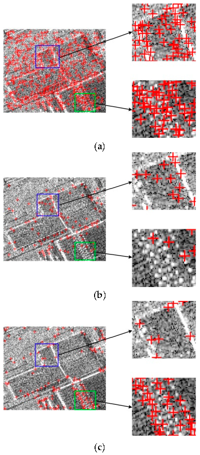
Figure 1a shows that a lot of noise was detected as interest points falsely by the DoG detector. Figure 1b shows the result of the improved DoG detector adopted in [14,15,16]. The blue and green partially enlarged details show that false detection still exists and that many real feature points are overlooked, respectively. These results demonstrate that the improved DoG detector will suppress image noise and detail information at the same time. The result of the proposed method is shown in Figure 1c. Compared with the previous two methods, our method has a tendency to find highly matchable interest points and avoids the noise normally brought by other methods. Table 1 shows the repeatability rate of interest points detected by the three detector in a pair of registered TerraSAR-X (X band, HH polarization) image and Quickbird panchromatic image. It is observed that the proposed detector achieves the highest repeatability rate. In the test, two points from different images with a Euclidean distance smaller than two pixels are regarded as repeated points.

2.2. GGS Bi-Windows-Based Feature Descriptor Computation

2.2.1. Local Support Region Size and Orientation Determination for Interest Points

In remote sensing applications, the input images usually have been approximately geo-referenced using the star-sensor so that the top and bottom of the images point to north and south of the earth, thus there is only small rotation change between the SAR and optical images. Based on this observation, we do not compute a dominant orientation for each feature as the original SIFT method. This strategy can not only speed up the computation but also improve the matching performance [14,15,16]. In addition, the feature local region size is determined on the basis of image resolution instead of feature scale values. For each feature on the image with resolution ${\lambda }_1$, the radius of local support region is set as $r_1$. The local support region radius of each feature on another image with resolution ${\lambda }_2$ is set as $r_1\cdot {\lambda }_1/{\lambda }_2$.

2.2.2. GGS Bi-Windows-Based Gradient Operator

Gradient operators based on grayscale difference are sensitive to image noise. Recently, many ratio-based operators with a constant false alarm rate for SAR images have been proposed [30,31,32]. However, the rectangular bi-windows used in these operators have low performance in the 2D smoothing of filters and may produce unwanted high-frequency components under the influence of speckle noise in SAR images. Fortunately, GGS bi-windows can repair the defect of rectangular bi-windows [25]. For each pixel, the local means in the GGS bi-windows are computed as follows:

$$m\left(x,y|\theta \right)={\displaystyle \sum _{\left(x\prime ,y\prime \right)}{W}^{\theta }\left(x\prime ,y\prime \right)I\left(x-x\prime ,y-y\prime \right)},$$

(6)

where $\theta =0,\pi /P,\cdots ,\pi (P-1)/P$ is the orientation angle of GGS bi-windows in order to detect different direction edges; $P$ is the number of orientations; $W^{\theta }$ is window function with an orientation angle $\theta$. The window function in the horizontal bi-window is defined as follows:

$$W\left(x,y\right)=\frac{{\left|y\right|}^{\alpha -1}\exp \left[-\left(\frac{x^2}{2{\sigma }^2}+\frac{\left|y\right|}{\beta }\right)\right]}{\sqrt{2\pi }\sigma \Gamma \left(\alpha \right){\beta }^{\alpha }},$$

(7)

where $\sigma$ is a parameter to control the window length; $\alpha$ is to control the window width; $\beta$ is to control the spacing of the two windows. The window function is Gaussian-shaped at the horizontal orientation and Gamma-shaped at the vertical orientation.

On the basis of the above local mean computation, we define the GGS bi-windows-based horizontal and vertical gradient operator as follows:

$$g_x=\ln \frac{m_1\left(x,y|\pi /2\right)}{m_2\left(x,y|\pi /2\right)},g_y=\ln \frac{m_1\left(x,y|0\right)}{m_2\left(x,y|0\right)},$$

(8)

where $g_x$ is the horizontal gradient; $g_y$ is the vertical gradient; $m_1(x,y|\pi /2)$, $m_2(x,y|\pi /2)$, $m_1(x,y|0)$, and $m_2(x,y|0)$ are the local means in the GGS bi-windows at orientation $\pi /2$ and 0.

The gradient magnitude $G_m$ and orientation $G_{\theta }$ are defined as follows:

$$G_m=\sqrt{g_x^2+g_y^2},\begin{array}{cc}& G_{\theta }=\end{array}\{\begin{array}{l}\arctan \left(g_y/g_x\right),G_{\theta }\le \pi \\ \arctan \left(g_y/g_x\right)-\pi ,otherwise\end{array}.$$

(9)

The gradient orientation is normalized in the range of $[0,\pi )$ and then classified into eight subintervals, which make the gradient robust to the non-linear grayscale differences between SAR and optical images.

Some comparison experimental results of the traditional gradient operators [8,17] and the proposed gradient operator are shown in Figure 2. The experimental results show that both the magnitude and orientation between the SAR and optical images computed by the proposed gradient operator present higher similarity than those of the other two gradient operators.

2.2.3. Feature Descriptor Construction

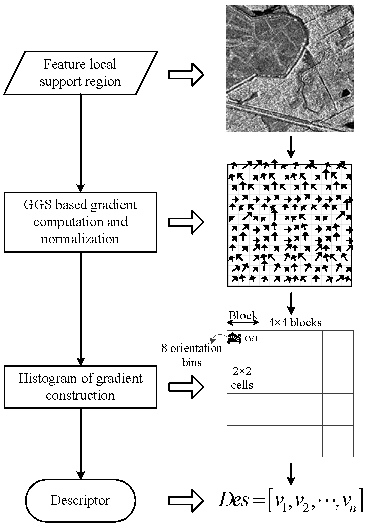
In this paper, the proposed GGS bi-windows-based gradient operator is combined with the HOG pattern to construct the feature descriptor. First, the gradient magnitude and orientation of each pixel in the feature local support region are computed and normalized. Second, the local support region is divided into several blocks and each block is further divided into several cells. Thereafter, the histogram of gradient orientation is constructed for each block and cell. Finally, all histograms are combined to generate a descriptor. To improve the robustness for grayscale change, the descriptor is normalized. The flow chart of descriptor computation is shown in Figure 3.

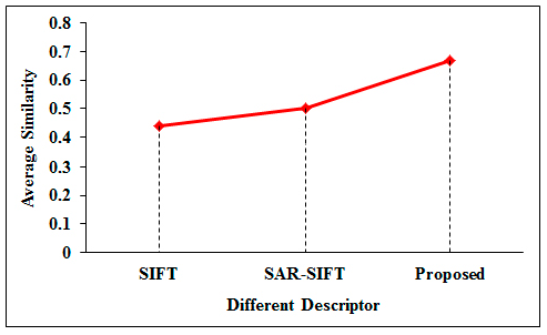
A group of experimental results based on the indicator “Similarity” in Equation (10) to evaluate the SIFT descriptor, SAR-SIFT descriptor and the proposed descriptor are shown in Figure 4. In the experiments, the detector proposed in Section 2.1 is adopted to find interest points in the SAR image shown in Figure 2a. And points in the optical image in Figure 2a with the same coordinates of the interest points in the SAR image are regarded as the correspondences since the two images are precisely registered previously. Then, the three descriptors are used to compute feature descriptor for each interest point.

The indicator “Similarity” is defined as:

$$Similarity=\exp \left(-\frac{{\displaystyle \sum _{i=1}^{m}dist(descSA{R}_i-descOp{t}_i)}}{m}\right),$$

(10)

where m is the number of interest points. $descSA{R}_i$ denotes the normalized descriptor of the i^th interest point in the SAR image. $descOp{t}_i$ denotes the normalized descriptor of the correspondence in the optical image. $dist()$ is a function to compute the square root of the sum of squares of all elements in a vector. $\exp ()$ is a function to compute the exponent.

Experimental results in Figure 4 show that higher similarity is obtained by the proposed descriptor between correspondences compared with the other two descriptors. It demonstrates the better performance of the proposed descriptor.

2.3. Image Matching Based on Descriptor Similarity and Geometric Constraint

Given that the image is rectified previously and image spatial resolution is known in most applications, some geometric relationships can be used to constrain the matching procedure. A matching framework based on the strategy in [16] is adopted in this paper:

First, the similarities between feature descriptors are computed using the Euclidean distance.

Second, the K-NN strategy is used to find K candidates for each feature in the reference image on the basis of descriptor similarity because the large differences between SAR and optical images may lead to some true correspondences without the largest similarity. Correspondence candidates are marked as $(C_i^{sar},C_i^{optical})$, $(i=1,\cdots ,I)$, where I is the number of correspondence candidates. This number is K times of the number of features on the reference image. Among the candidate pairs, the H pairs with the largest descriptor similarity, i.e., with the smallest descriptor distance, are set as seed match pairs $M_h,(h=1,\cdots ,H)$.

Third, a match set $S_h$ is constructed for each seed match pair $M_h$. Each pair of correspondence in $S_h$ is marked as $(F_j^{sar},F_j^{optical}),(j=1,\cdots ,J)$, where $J$ is the number of correspondences in $S_h$. At the beginning, $M_h$ is saved in $S_h$ and regarded as the reference. Then, each candidate in the initial correspondence set is compared with all correspondences in $S_h$.

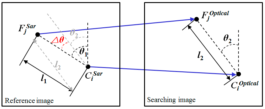
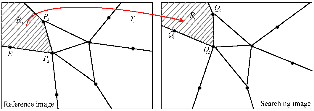
As shown in Figure 5, for a pair of candidate match $(C_i^{sar},C_i^{optical}),(i=1,\cdots ,I)$ and a pair of reference match $(F_j^{sar},F_j^{optical}),(j=1,\cdots ,J)$, if the difference between the distance ratio $l_1/l_2$ and the image resolution ratio ${\lambda }_2/{\lambda }_1$ is smaller than a threshold $t_d$, and the difference between the angles ${\theta }_1$ and ${\theta }_2$ is smaller than a threshold $t_{\theta }$, this pair of candidate match is regarded as spatially consistent with the reference match. When the candidate is checked by all reference matches in $S_h$, if the candidate match is spatially consistent with more than 95% reference matches, it is saved into $S_h$. Different from the distance ratio constraint based on an estimated scale factor in [16], the scale factor is replaced by image spatial resolution ratio in our experiments.

Finally, iterative computation is performed for each seed match and the iteration that generates the $S_h$ with most matches is identified. Matches in the set $S_h$ are considered as initial matches, which are then saved into a set $S_M$.

2.4. Outliers Elimination

Outliers are inevitably present in the previous set of correspondences $S_M$. Traditional methods estimate the homography between images by using the RANSAC algorithm. Matches that do not conform to the homography will be eliminated as outliers. However, the local distortions of SAR images, e.g., foreshortening, lay over and shadowing, make the geometric transformation between all pixels of two images cannot be approximated to an affine transform. Therefore, many correct matches will be eliminated as outliers under the homography constraint. To overcome this problem, polynomials of degree two, as shown in Equation (11), are combined with the extension of Denaulay triangles [33] to construct a whole-to-local constraint framework in the proposed method.

$$\{\begin{array}{c}{x}_1=a_0+a_1{x}_2+a_2{y}_2+a_3{x}_2^2+a_4{x}_2{y}_2+a_5{y}_2^2\\ y_1=b_0+b_1{x}_2+b_2{y}_2+b_3{x}_2^2+b_4{x}_2{y}_2+b_5{y}_2^2\end{array},$$

(11)

where $(x_1,y_1)$ and $(x_2,y_2)$ are the coordinates of matches in the reference image and searching image, respectively. $a_0,\cdots ,a_5$ and $b_0,\cdots ,b_5$ are the polynomial coefficients.

The procedure of outliers elimination is as follows:

Step 1:

Select six correspondences from $S_M$ randomly to construct a sample set.

Step 2:

Compute the polynomials of degree two with the current sample set.

Step 3:

Test all matches in $S_M$ by using the polynomials and save the correspondences with residuals smaller than a threshold (e.g., 1 pixel) into a set $S_p$.

Step 4:

Perform iterative computation. If the correspondences in the current set $S_p$ are more than the correspondences in the previous set, the current polynomials and correspondences set $S_p$ are preserved. The previous polynomials and set $S_p$ are discarded.

Step 5:

After the iterative calculation, matches in the final correspondence set $S_p$ are regarded as correct matches.

Step 6:

The extension Delaunay triangles are constructed in each image based on points in the final $S_p$. The images are divided into sub-regions.

Step 7:

A local transformation $H_i$ is fitted for each pair of corresponding sub-regions based on the matches in the sub-regions from the initial matches set $S_M$. For each initial match, if the position transformation error based on $H_i$ is larger than two pixels, it is regarded as false match.

The detailed local transformation fitting processing is shown in Figure 6. The affine transformation $T_i$ between each pair of corresponding sub-regions $R_i$ and $R_i^{\prime }$ is computed based on the corresponding three pairs of matches that compose the sub-regions. Then, we use $T_i$ to check the matches in the sub-regions from set $S_M$ and count the number of matches consistent with $T_i$. If the number is larger than six, $H_i$ is set as polynomials of degree two shown in Equation (11); if the number is smaller than six and larger than three, $H_i$ is set as affine transformation shown in Equation (12); otherwise, the initial matches in $R_i$ and $R_i^{\prime }$ are clustered into other sub-regions according to the Euclidean distance and they will be checked by the sub-regions they clustered into.

$$\{\begin{array}{c}{x}_1=a_0+a_1{x}_2+a_2{y}_2\\ y_1=b_0+b_1{x}_2+b_2{y}_2\end{array},$$

(12)

where $(x_1,y_1)$ and $(x_2,y_2)$ are the coordinates of matches in the reference image and searching image, respectively. $a_0,a_1,a_2$ and $b_0,b_1,b_2$ are the transformation coefficients.

3. Experimental Results and Discussion

3.1. Experimental Datasets

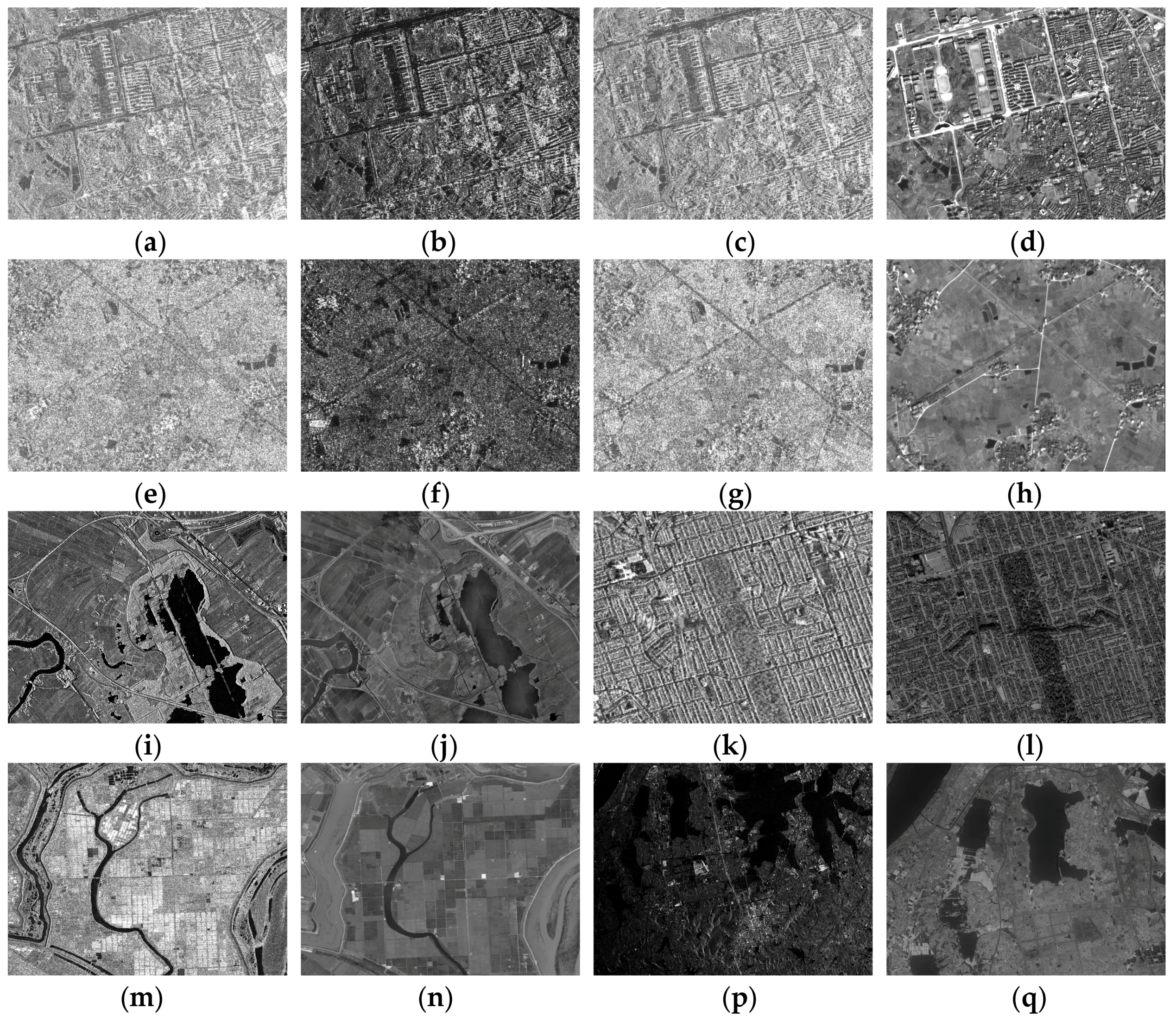
The proposed method is compared with SIFT [8] and other methods proposed by Schwind [14], Suri [15], Fan [16], and Dellinger (SAR-SIFT) [17] on the basis of the images shown in Figure 7. For convenience, some of the comparative methods are labeled as the name of the first author. Among the datasets, the SAR images include COSMO-Skymed (X band, HH polarization), RADARSAT-2 (C band, HH polarization), TerraSAR-X (X band, HH polarization) and HJ-1C (S band, VV polarization) images. The optical images include ZY-3 images and Google Earth images.

On the basis of the images in Figure 7, 12 pairs of images are grouped. The detailed information of the image pairs are shown in

Table 2. Description of image pairs used in the experiments.

Category	Pair Number	Image Number	Image Source	Image Size (Unit: Pixel)	Spatial Resolution (Unit: Meter)
SAR & SAR	Pair 1	(a)	COSMO-Skymed	724 × 951	2.70
		(b)	RADARSAT-2	848 × 1114	2.30
	Pair 2	(f)	RADARSAT-2	497 × 642	2.30
		(g)	TerraSAR-X	592 × 765	1.85
SAR & Optical	Pair 3	(a)	COSMO-Skymed	724 × 951	2.70
		(d)	ZY-3	934 × 1227	2.10
	Pair 4	(b)	RADARSAT-2	848 × 1114	2.30
		(d)	ZY-3	934 × 1227	2.10
	Pair 5	(c)	TerraSAR-X	1011 × 1328	1.85
		(d)	ZY-3	934 × 1227	2.10
	Pair 6	(e)	COSMO-Skymed	424 × 584	2.70
		(h)	ZY-3	547 × 707	2.10
	Pair 7	(f)	RADARSAT-2	497 × 642	2.30
		(h)	ZY-3	547 × 707	2.10
	Pair 8	(g)	TerraSAR-X	592 × 765	1.85
		(h)	ZY-3	547 × 707	2.10
	Pair 9	(i)	TerraSAR-X	715 × 1073	1.85
		(j)	Google Earth	715 × 1073	1.85
	Pair 10	(k)	TerraSAR-X	1165 × 1315	1.75
		(l)	Google Earth	1699 × 1918	1.19
	Pair 11	(m)	TerraSAR-X	1751 × 2030	2.75
		(n)	Google Earth	986 × 1351	4.78
	Pair 12	(p)	HJ-1C	2450 × 3575	5.00
		(q)	ZY-3	1600 × 2000	4.60

. Both the reference image and searching image in the first two pairs are SAR images. In the other 10 pairs, all reference images are SAR images and all searching images are optical images. Therefore, all the matching experiments in this paper can be classified into two groups: the first group is used to compare the performance of each method for SAR and SAR images; the second group is used to evaluate the matching performance for SAR and optical images.

3.2. Evaluation Criteria

Two indicators, number of correct matches (NCM) and matching precision (MP), are adopted to evaluate the performance of each matching method. MP is computed as MP = (NCM/M) × 100%, where M is the number of total matches. To count the correct matches, 50 evenly distributed correspondences are selected manually and the projective transformation is calculated for each pair of images. Then, those matches with localization errors smaller than two pixels based on the global consistency of the projective transformation are regarded as correct matches.

3.3. Thresholds Setting

In the proposed method, those thresholds affecting the final matching performance are listed in

Table 3. Thresholds of the proposed method.

Thresholds	Description
$r_1$	local support region radius of features in the image with spatial resolution ${\lambda }_1$
$\sigma$	to control the length of the GGS bi-windows
$\alpha$	to control the width of the GGS bi-windows
$\beta$	to control the spacing between the two windows of the GGS bi-windows
$K$	the number of initial candidate correspondences for each interest point in the SAR image
$H$	the number of seed matches
$t_d$	the distance ratio threshold of the geometric constraint in the matching strategy
$t_{\theta }$	the orientation difference threshold of the geometric constraint in the matching strategy

.

In the experiments, the last four parameters are set as $K=25$, $H=10$, $t_d=0.2$ and $t_{\theta }=5^{°}$, according to the recommendation in [16]. The first four parameters are tuned as follows.

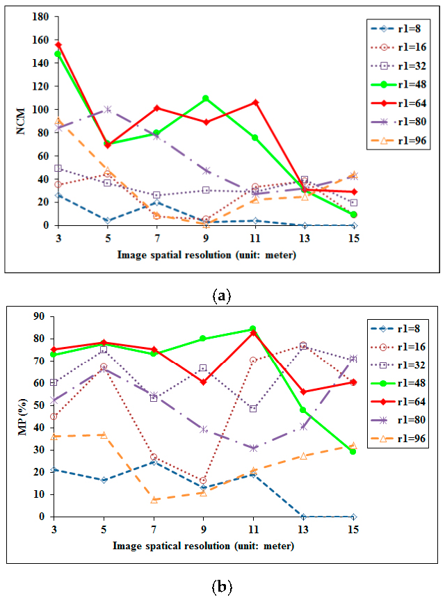
3.3.1. Tuning of Feature Local Support Region Radius $r_1$

Firstly, several simulated datasets are constructed. In the experiments, we use each image pair from pair 3 to pair 11 in Table 2 to simulate a dataset. Each original image pair is manually registered before simulation. The simulation is performed by using Gaussian smooth and downsampling. After the simulation, each dataset contains seven pairs of images with resolution 3 m, 5 m, 7 m, 9 m, 11 m, 13 m, and 15 m. Then, these 10 datasets with 77 pairs of images together are used to tune the parameter of feature local support region radius. Because it is observed that all groups of tests show similar tuning results, here only one group (based on image pair 11) is displayed. The detailed information on the dataset simulated from image pair 11 is shown in

Table 4. Information of the dataset simulated from image pair 11.

Number of Simulated Image Pair	Spatial Resolution (Unit: Meter)	Image Size (Unit: Pixel)
1	3.00	1000 × 1000
2	5.00	689 × 681
3	7.00	654 × 670
4	9.00	664 × 681
5	11.00	515 × 538
6	13.00	468 × 463
7	15.00	403 × 405

.

In this part, in order to test the effect of feature local support region radius to the matching performance, all other parameters are regarded as constant. Besides the geometric constraint parameters described before, the parameters of the GGS bi-windows are set as: $\sigma =3.7$, $\alpha =3$, and $\beta =1.5$. The computed NCM and MP values of all images pairs are shown in Figure 8.

From the experimental results, it can be seen that both too small a local support region and too large a local support region produced low NCM and MP values. There are two reasons: firstly, too small a region makes the descriptor not robust to image noise and grayscale difference. Also, it leads to low similarity between the descriptors of correspondence. Secondly, too large a region decreases the distinction of the feature descriptor, which makes it difficult to distinguish the descriptors of non-correspondence and find false matches. From the results, it is observed that the overall peak performance of NCM and MP have been obtained when the region radius $r_1$ is set at 64 pixels. Therefore, the threshold is set at 64 pixels in the following experiments.

3.3.2. Tuning of GGS Bi-Windows Thresholds

There are three thresholds, $\sigma$ to control the window length, $\alpha$ to control the window width, and $\beta$ to control the spacing between windows, can affect the performance of the GGS gradient operator and the final matching result. When we are tuning one parameter, the other two parameters are set as constant as the tuning of feature local support region radius. 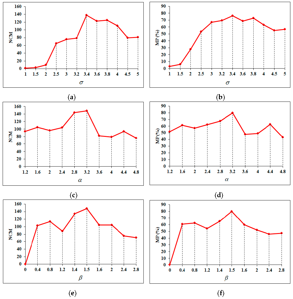The tuning of these three thresholds is performed based on the 11 SAR and optical image pairs in Table 2. Because it is observed that all tests show similar tuning results, here only the result based on image pair 11 is displayed. The experimental results are shown in Figure 9.

Among the three thresholds, $\sigma$ is tuned firstly. In the tuning of $\sigma$, other two parameters $\alpha$ and $\beta$ are set at 3 and 1.5, respectively. From Figure 9a,b, it can be observed that the best matching performance is obtained when $\sigma =3.4$. Therefore, in the tuning of other two parameters, $\sigma$ is set as 3.4. $\alpha$ is tuned secondly. In that tuning, $\beta$ is set as 1.5. And from Figure 9c,d, we can see that the best matching performance is obtained when $\alpha =3.2$. Therefore, in the tuning of $\beta$, other two thresholds $\sigma$ and $\alpha$ are set as 3.4 and 3.2, respectively. From Figure 9e,f, it can be seen that the best matching performance is obtained when $\beta =1.5$.

Based on the experiments and analysis in this section, all thresholds in the proposed matching method are set as in

Table 5. Threshold setting of the proposed method.

Thresholds
$r_1$	$\sigma$	$\alpha$	$\beta$	$K$	$H$	$t_d$	$t_{\theta }$
64	3.4	3.2	1.5	25	10	0.2	$5^{°}$

.

3.4. Descriptors Comparison

In order to evaluate the performances of different descriptors, the interest point detector described in Section 2.1 and the NNDR matching strategy of the three descriptors are combined to match the 12 pairs of images listed in Table 2. All descriptors are computed in a feature support region with fixed radius (64 pixels) and orientation (0 degree). The matching performances of different descriptor based methods are shown in

Table 6. NCM and MP values of different descriptor based matching methods.

Image Pair	SIFT		SAR-SIFT		Proposed
	NCM	MP	NCM	MP	NCM	MP
Pair 1	0	0.0%	0	0.0%	2	11.1%
Pair 2	1	10.0%	1	50.0%	2	50.0%
Pair 3	0	0.0%	0	0.0%	1	20.0%
Pair 4	0	0.0%	0	0.0%	2	33.3%
Pair 5	0	0.0%	1	20.0%	1	5.3%
Pair 6	0	0.0%	1	33.3%	3	50.0%
Pair 7	0	0.0%	1	25.0%	4	44.4%
Pair 8	0	0.0%	1	33.3%	3	37.5%
Pair 9	51	67.8%	21	75.0%	58	69.0%
Pair 10	0	0.0%	0	0.0%	1	7.7%
Pair 11	1	16.7%	1	33.3%	5	41.7%
Pair 12	1	20.0%	2	28.6%	5	22.7%

.

It is observed from Table 6 that the matching method based on the proposed descriptor performs best for almost all the image pairs. Although the SAR-SIFT descriptor-based method achieves slightly higher matching precision than the proposed method for some image pairs, it obtains fewer correct matches than the proposed method. The SIFT descriptor-based method almost fails for most image pairs except pair 9. It works much better in 9 than in other image pairs because the radiometric difference between the images in pair 9 is not as significant as that in other pairs. In this comparison, the same detector and matching strategy without geometric constraint are selected for all matching methods. Therefore, the test results can fairly reflect the performances of different descriptors.

3.5. Matching Strategies Comparison

In order to evaluate the performance of the applied matching strategy in the proposed method, we compare it with the NNDR method, the fast sample consensus (FSC) method [34] and the enhanced matching method (EM) [35]. The interest point detector and descriptor described in Section 2.1 and Section 2.2 are adopted to extract features for all four matching methods. The KNN candidates are selected as the input of all methods. The test is based on the 12 image pairs listed in Table 2. The statistic matching results of the four matching strategies are shown in

Table 7. NCM and MP values of different matching strategies.

Image Pair	NNDR		FSC		EM		GC
	NCM	MP	NCM	MP	NCM	MP	NCM	MP
Pair 1	2	11.1%	0	0.0%	0	0.0%	75	21.4%
Pair 2	2	50.0%	0	0.0%	0	0.0%	76	30.6%
Pair 3	1	20.0%	0	0.0%	0	0.0%	46	51.7%
Pair 4	2	33.3%	0	0.0%	0	0.0%	113	24.6%
Pair 5	1	5.3%	0	0.0%	0	0.0%	137	30.4%
Pair 6	3	50.0%	6	66.7%	8	72.7%	33	42.3%
Pair 7	4	44.4%	5	62.5%	9	75.0%	25	41.7%
Pair 8	3	37.5%	7	63.6%	13	76.5%	60	49.2%
Pair 9	58	69.0%	73	96.0%	98	100.0%	489	69.7%
Pair 10	1	7.7%	0	0.0%	0	0.0%	118	39.2%
Pair 11	5	41.7%	12	63.2%	26	65.0%	155	33.6%
Pair 12	5	22.7%	16	64.0%	37	74.0%	432	38.5%

. The adopted matching strategy based on geometric constraint is labeled GC in this comparison.

It is observed from Table 7 that the GC strategy adopted in the proposed method obtained many more correct matches than the other matching strategies for all image pairs. The MP values of other methods are higher than the GC method in some cases, but the few correct matches cannot meet the demands of some applications. The NNDR strategy computes the descriptor distance ratio to find matches. Unfortunately, for SAR and optical images, many correspondences that are expected to be matched do not meet the distance ratio constraint, or do not even have the minimum descriptor distance. Therefore, the number of correct matches of NNDR is limited. In addition, we can see that the matching performances of the FSC and EM methods are unstable. For example, they work very well for image pair 9 but fail for some other image pairs. This is because the NNDR result is part of the input of the FSC and EM methods. They will work well if the NNDR method works and at least three correct matches are obtained to compute the initial transformation. Otherwise, they will fail. In the GC method, the input is the K-NN result. Most of the correspondences expected to be matched are contained in the K-NN result. During the iteration, the GC method can work well if one correct match is found. This is a requirement easy to meet. Therefore, the GC method is more stable than other methods.

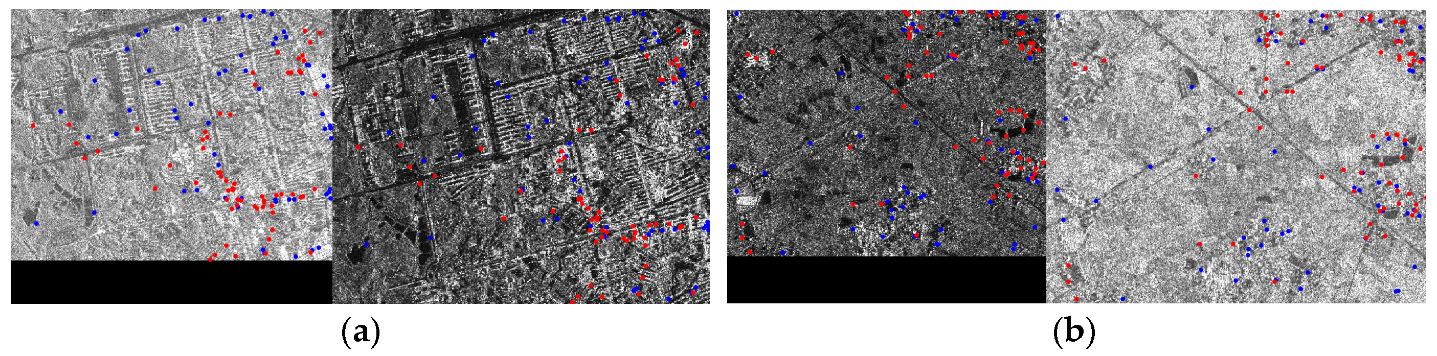
3.6. Matching Performances of Different Framework between SAR and SAR Images

In this part, the proposed method is compared with other methods on the first two pairs of images shown in Table 2. The corresponding NCM and MP values are shown in

Table 8. NCM values of each method for SAR and SAR images.

Image Pair	Matching Methods
	SIFT	Schwind	Suri	Fan	SAR-SIFT	Proposed
Pair 1	0	0	2	5	4	75
Pair 2	1	2	3	7	5	76

and

Table 9. MP values of each method for SAR and SAR images.

Image Pair	Matching Methods
	SIFT	Schwind	Suri	Fan	SAR-SIFT	Proposed
Pair 1	0.0%	0.0%	16.7%	6.1%	1.8%	46.8%
Pair 2	4.8%	20.0%	33.3%	36.8%	31.3%	50.7%

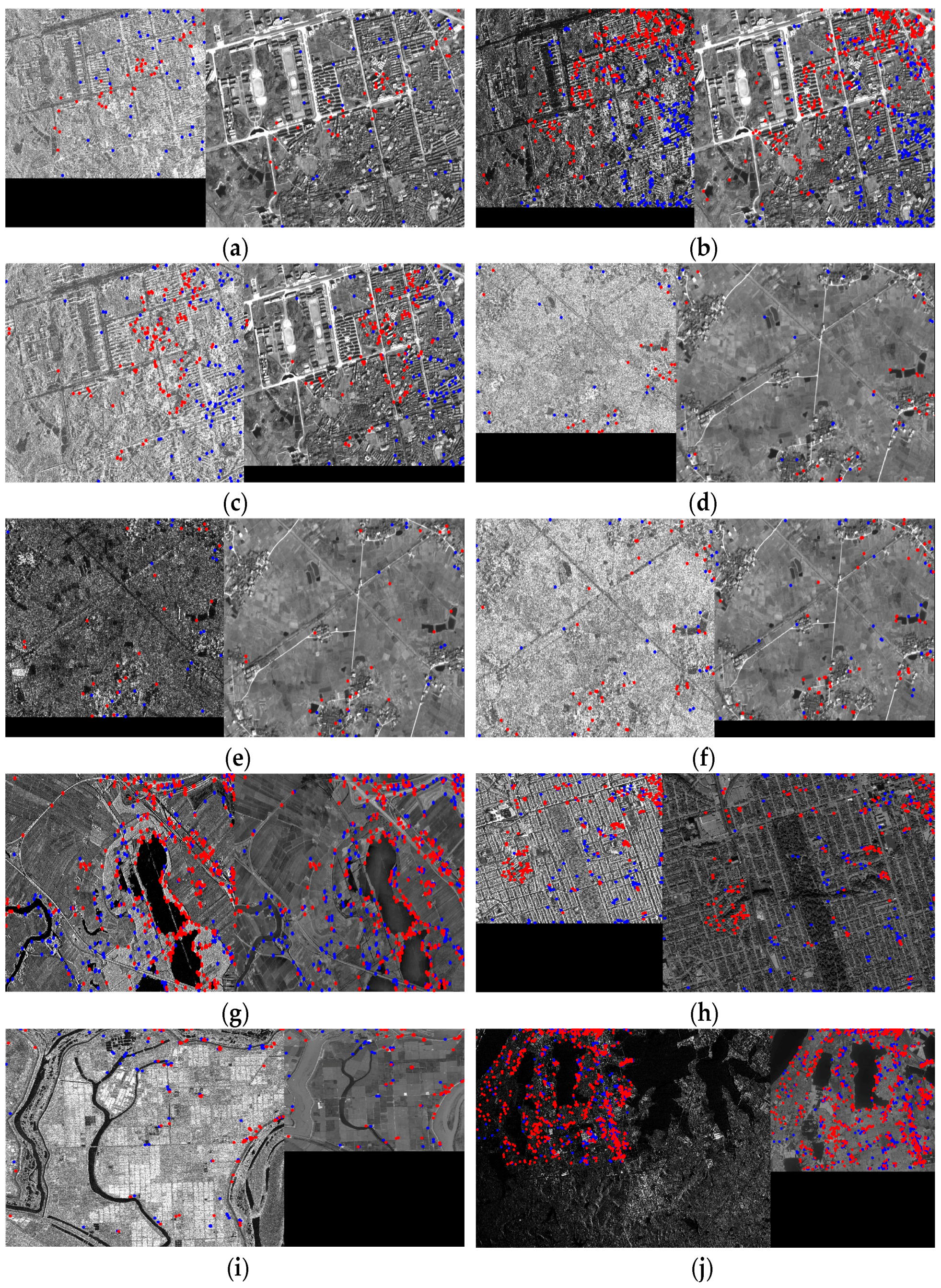
, and the matching results of the proposed method are illustrated in Figure 10.

Table 8 shows that the proposed method obtained more correct matches than the other methods because of the use of ratio-based gradient operators. By replacing the rectangular windows with GGS bi-windows and using geometric constraints, the proposed method becomes much more robust to image noise and can achieve better performance than the SAR-SIFT method. Furthermore, other methods, particularly Fan’s method, can also obtain several matches. Two reasons contribute to this result. First, all images in the first and second pairs are SAR images, and many noise correspondences exist between images. Some matches in the results of these methods are not the expected feature correspondences. Secondly, the slight grayscale difference between SAR and SAR images is acceptable for these methods. Table 9 shows that the proposed method not only obtains many more correct matches, but also reaches higher matching precision than all the other methods. It also shows a similar result to the NCM: Fan’s method obtained the second best performance, behind the proposed method, which benefited from the contribution of the geometric constraint.

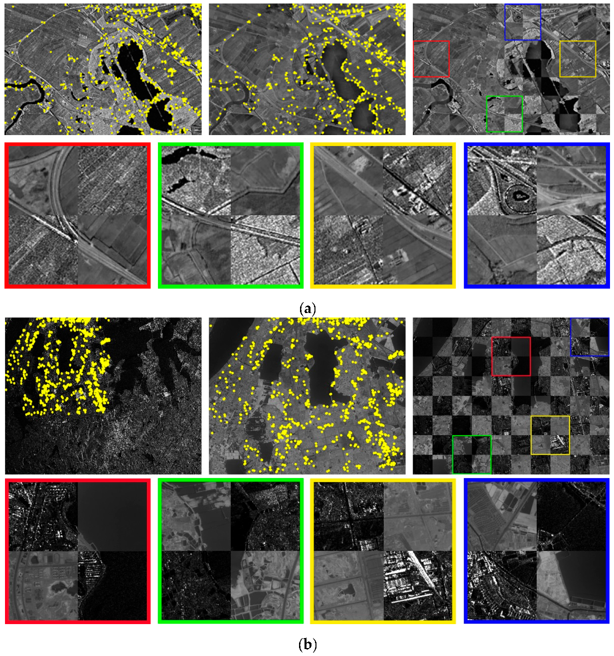
3.7. Matching Performances of Different Framework between SAR and Optical Images

Different from matching SAR and SAR images, methods for matching SAR and optical images should be robust to image noise and non-linear grayscale difference. In this section, the proposed method is compared with the other methods on the basis of image pairs 3–12, described in Table 2. The NCM and MP values of each method are shown in

Table 10. NCM values of each method for SAR and optical images.

Image Pair	Matching Methods
	SIFT	Schwind	Suri	Fan	SAR-SIFT	Proposed
Pair 3	0	0	2	0	0	46
Pair 4	0	0	1	0	4	113
Pair 5	0	0	0	0	2	137
Pair 6	0	0	0	4	1	33
Pair 7	0	0	0	13	4	25
Pair 8	1	1	0	1	5	60
Pair 9	29	20	39	14	58	489
Pair 10	0	0	0	0	0	118
Pair 11	1	1	2	0	1	155
Pair 12	5	10	5	174	9	432

and

Table 11. MP values of each method for SAR and optical images.

Image Pair	Matching Methods
	SIFT	Schwind	Suri	Fan	SAR-SIFT	Proposed
Pair 3	0.0%	0.0%	9.1%	0.0%	0.0%	57.5%
Pair 4	0.0%	0.0%	3.7%	0.0%	4.2%	59.2%
Pair 5	0.0%	0.0%	0.0%	0.0%	2.2%	72.1%
Pair 6	0.0%	0.0%	0.0%	36.4%	25.0%	68.8%
Pair 7	0.0%	0.0%	0.0%	43.3%	40.0%	62.5%
Pair 8	2.3%	8.3%	0.0%	5.9%	41.7%	76.9%
Pair 9	25.9%	43.5%	47.0%	19.2%	55.2%	75.2%
Pair 10	0.0%	0.0%	0.0%	0.0%	0.0%	59.0%
Pair 11	0.1%	0.7%	1.1%	0.0%	6.7%	67.4%
Pair 12	1.0%	5.1%	2.1%	19.8%	21.4%	71.4%

, respectively. The matching results of the proposed method are illustrated in Figure 11. In this part, we also tuned the thresholds discussed in Section 3.3. The best matching results are obtained based on the threshold values shown in Table 5, consistent with the conclusion in Section 3.3.

Experiments in Table 10 and Table 11 show that in all tests the proposed method improves the matching performance significantly compared with other methods. There are several reasons contributing to the improvement: first, the interest point detector used in the proposed matching method can find features with higher localization accuracy, as shown in Figure 1. Most of the detected interest points are located at “real features”. These features are more salient than those features detected by other methods. It is easier to find correspondences for features with high distinctiveness; second, the GGS bi-windows based gradient operator in the proposed method is more robust to noise and non-linear grayscale changes between SAR and optical images. This makes the feature descriptors of correspondences have high similarity and the descriptors of non-correspondences have high distinctiveness. It is a fundamental property for a good image matching method; third, the determination of feature local support region radius and feature orientation is based on image spatial resolution and the property of rectified remote sensing images. This strategy improves the reliability of feature local support region size and orientation; fourth, the geometric constraint in the matching framework reduces the searching area. The interference of those features with similar descriptors is avoided. Moreover, the whole to local outlier elimination method further improves the matching precision.

The first three methods, SIFT, Schwind’s method, and Suri’s method, almost fail to match these images because of the following reasons. In SIFT method, firstly, the DoG detector is sensitive to noise and much speckle noise is detected as features in SAR images. However, there is no corresponding noise in the optical images. Therefore, the noise affects the matching and produces many outliers. Secondly, the computed scale values and orientation in the SIFT method are unstable and the local support regions to compute feature descriptors are inconsistent between correspondences. It is difficult to extract similar descriptors from this kind of feature support region. Thirdly, the gradient operator used in the SIFT method is sensitive to image noise and non-linear grayscale changes between SAR and optical images. It makes the SIFT descriptors of correspondences between SAR and optical images have low similarity and produces false matches. Finally, the nearest neighbor distance ratio (NNDR) matching strategy in the SIFT method is unreliable because of the low similarity between the descriptors of correspondences and the low distinctiveness between the descriptors of non-correspondences. In Schwind’s method, although the influence of image noise is reduced by detecting features from the second octave of the image pyramid, many salient features with high localization accuracy on the first octave are eliminated. Except for the processing of image noise, the other problems with the SIFT method are still not solved in this method. Based on Schwind’s method, a certain orientation (0 degree) is assigned to each feature in Suri’s method. However, other problems—unstable scale computation, a sensitive gradient operator, and an unreliable matching strategy—are still not solved. Fan added a geometric constraint to the method based on the spatial relationship between correspondences to improve the matching performance. From the experimental results, it can be observed that this kind of geometric constraint works very well. However, the improvement is limited because of the unstable scale value computation and gradient operator. In addition, the reference scale ratio in the geometric constraint in Fan’s method is computed from the initial matches, which is less reliable compared with the determination based on image spatial resolution in the proposed method.

SAR-SIFT is a new kind of method. The grayscale difference-based gradient operator is replaced with a ratio-based gradient operator, which contributes to obtain a similar descriptor between SAR and SAR images. This key improvement promotes the method, obtaining the second-best performance overall. However, the operator will generate some unexpected strong responses around local features because of the rectangular windows. This method is designed for matching between SAR images; the non-linear grayscale difference between the SAR and optical images will affect the matching performance. Moreover, the problems of unstable scale value and orientation computation and the unreliable matching strategy mean that the method cannot obtain satisfactory results in many applications.

All the comparative methods obtained more correct matches for image pairs 9 and 12 than other image pairs because some objects in the SAR and optical images of the two pairs have similar grayscale distribution. For example, some lakes and rivers exist in these image pairs. It can be seen that the lakes and rivers appear as lower grayscale levels than the other objects around them in both the SAR and optical images of the two pairs. This makes the pixels along the lakeside and riverside have the same gradient orientation and produces similar feature descriptors in the SAR and optical images. Therefore, some correct matches have been obtained in these regions.

3.8. Registration Accuracy

In this study, image registration accuracy is adopted to evaluate the matching performance, in addition to NCM and MP. Image registration is performed on the basis of the matching results of each method. For the proposed method, we use the matches after the constraint of the initial polynomials of degree two to construct extension Delaunay triangles. Then, local registration is implemented for each sub-region based on the polynomials of degree two in Equation (11) if the number of matches in the sub-region is greater than six. Otherwise, the local registration is implemented based on the affine transformation in Equation (12). For other comparative methods, we use all the matches to construct extension Delaunay triangles. Local registration is implemented for each sub-region based on the three pairs of matches constructing the sub-region. Registration accuracy is measured by using the root mean square error (RMSE), which is computed as follows on the basis of manually selected ground control points on the registered images:

$$RMSE=\sqrt{\frac{1}{n}{\displaystyle \sum _{i=1}^n\left[{\left(x_i-x_i^{\prime }\right)}^2+{\left(y_i-y_i^{\prime }\right)}^2\right]}},$$

(13)

where $(x_i,y_i)$ and $(x_i^{\prime },y_i^{\prime })$ is a pair of correspondence and n is the number of selected correspondences. In the experiments, n is set at 50.

Given that all matching methods mentioned in this paper can obtain more than three pairs of correct matches on image pairs 9 and 12, the registration accuracy is evaluated on the two pairs of images. The experiment results are shown in

Table 12. Root mean square error (unit: pixel).

Image Pair	SIFT	Schwind	Suri	Fan	SAR-SIFT	Proposed
Pair 9	2.15	2.53	2.39	2.27	1.47	1.01
Pair 12	3.43	3.19	2.03	1.74	1.22	0.88

.

Table 12 shows that the proposed method achieves the highest registration accuracy (near one-pixel accuracy), which can meet the requirements of many applications. For image pair 9, the RMSE values of the first four methods are beyond two pixels. This is because the localization accuracy of the DoG features in these methods is lower than that of the Harris features in SAR-SIFT and the phase congruency features in the proposed method. Especially for the methods of Suri, Schwind, and Fan, features are detected from the higher levels (smoothed images) of the pyramid, which further decreases the feature localization accuracy. For image pair 12, the registration accuracy of the first two methods is beyond three pixels. This is because these two methods obtained fewer correct matches and some image regions have no corresponding control points to rectify the local distortion. Compared with other methods, the proposed method obtained many more correct matches. These matches were evenly distributed on the images, which contributes to the precise registration of local distortion. The registration results based on the proposed matching method are shown in Figure 12. The visualization results also show that the registration is very accurate.

All the experimental results and analysis in this study show that the proposed method can address the problems in both SAR/SAR image matching and SAR/optical image matching better than the other methods.

4. Conclusions

In this paper, a robust matching method is developed to extract correspondences between SAR and optical images. Firstly, a phase congruency-based interest point detector is adopted to find corners with high localization accuracy under the influence of the speckle noises in SAR images because there is a noise factor designed to deal with image noise in the phase congruency function. However, image noise is regarded as additive noise in the phase congruency function. It is not robust to the speckle noise in SAR image. Therefore, a logarithmic transformation is applied to transform the speckle noise into additive noise in the SAR image. The visualization test results show that most of the interest points extracted by the proposed detector are located at “real features”. This is very important to improve the matching precision and registration accuracy because these features are more distinctive and easy to locate unambiguously. Secondly, a strategy of feature local support region radius and orientation determination is adopted based on the properties of remote sensing images to replace the feature local support region radius computation based on feature scale value and the orientation computation based on gradient. In most applications, images have been rectified already and the image spatial resolution is known. Thus, the proposed strategy can work well and is more reliable than the computation results in other traditional methods. Similar feature local support regions contribute to construct descriptors with high similarity between correspondences and produce good matching results. Thirdly, ratio-based gradient operator is more efficient to deal with noise in SAR images. The traditional rectangular bi-windows used in ratio-based gradient operators are replaced with GGS bi-windows. The GGS bi-windows can avoid unwanted high-frequency responses around real features, which is beneficial to construct a reliable descriptor. Meanwhile, the gradient orientation is normalized to obtain consistent orientations between correspondences under non-linear grayscale difference. Finally, a geometric constraint is combined with the descriptor similarity to compute feature matches. The geometric constraint reduces the search area and avoids the influence of those inconsistent features with high descriptor similarity. The popular NNDR strategy is not adopted in the proposed method because some correspondences between SAR and optical images that are expected to be matched correctly do not meet the descriptor distance ratio constraint in the NNDR strategy, or do not even have the most similar descriptors. After initial matching, an outlier elimination approach based on global and local constraints is proposed to further improve the matching precision. The experimental results in this paper demonstrate the effectiveness of the proposed method. However, we have to point out some drawbacks of the proposed method: firstly, in feature description, the adopted feature support region determination method will produce inconsistent feature areas for correspondences and generate false matches if there is significant topography in the scenes; secondly, the geometric constraint in the matching procedure and the polynomial fitting in the outlier elimination are global constraints that do not work well for scenes with significant topography; finally, the image resolution should be known and the images should have been roughly rectified when we plan to use the proposed method. One possible future study is to improve the matching performance of the proposed method for images with significant topography.