Article

Mapping 2000–2010 Impervious Surface Change in India Using Global Land Survey Landsat Data

by
Panshi Wang
1,*,
Chengquan Huang
1 and
Eric C. Brown de Colstoun
2
1
Department of Geographical Sciences, University of Maryland, College Park, MD 20742, USA
2
Biospheric Sciences Laboratory, NASA Goddard Space Flight Center, Greenbelt, MD 20771, USA
*
Author to whom correspondence should be addressed.
Remote Sens. 2017, 9(4), 366; https://doi.org/10.3390/rs9040366
Submission received: 1 February 2017 / Revised: 4 April 2017 / Accepted: 9 April 2017 / Published: 13 April 2017

Abstract

:
Understanding and monitoring the environmental impacts of global urbanization requires better urban datasets. Continuous field impervious surface change (ISC) mapping using Landsat data is an effective way to quantify spatiotemporal dynamics of urbanization. It is well acknowledged that Landsat-based estimation of impervious surface is subject to seasonal and phenological variations. The overall goal of this paper is to map 2000–2010 ISC for India using Global Land Survey datasets and training data only available for 2010. To this end, a method was developed that could transfer the regression tree model developed for mapping 2010 impervious surface to 2000 using an iterative training and prediction (ITP) approachAn independent validation dataset was also developed using Google Earth™ imagery. Based on the reference ISC from the validation dataset, the RMSE of predicted ISC was estimated to be 18.4%. At 95% confidence, the total estimated ISC for India between 2000 and 2010 is 2274.62 ± 7.84 km2.

Graphical Abstract

1. Introduction

The first decade of the twenty-first century witnessed rapid urbanization. More than half of the world’s population now dwells in urban areas, and the urban population is expected to reach two thirds of the world’s population by 2050 [1]. The physical manifestation of this global urbanization process on the Earth’s surface includes the conversion of forests, grasslands, and croplands to impervious surface (IS) cover. Impervious surface cover may alter the Earth’s environmental systems in many ways: areas covered by impervious surface may have a distinctive local climate, commonly known as the “urban heat island effect” [2,3]; hydrologic systems may be severely impacted as a result of increased runoff and degradation of water quality [4]; and urbanization is often associated with the loss of natural lands, which may have adverse implications for biodiversity and other ecosystem services [5,6] at local to regional scales. Moreover, recent studies on the linkages between urbanization and global environmental change have demonstrated that urbanization could have impacts beyond the physical footprint of urban areas [7].
However, monitoring urbanization as a process of impervious surface change (ISC) is an inherently difficult task. Impervious surface only covers a small percentage of the Earth’s land surface (estimates range from 0.2~3%) [8,9,10]. Also, urban areas are complex system in terms of both spatial variability of impervious surface cover density within the urban extent and temporal dynamics throughout the urbanization cycle [7,11,12].
Much effort has been made towards representing impervious surface/urban land cover in remote sensing based global maps. Such datasets include global land cover dataset with urban class [13,14,15], binary urban/non-urban maps [9,16,17], as well as continuous field impervious surface cover maps [18]. These datasets are produced using medium to coarse resolution data such as the Moderate Resolution Imaging Spectroradiometer (MODIS) and the Defense Meteorological Satellite Program Operational Linescan System (DMSP-OLS). Recently, 30 m resolution Landsat data started to be used for mapping urban areas globally [19,20]. Valuable as these datasets are, monitoring urbanization requires much more detailed data than the available global products. The complexity of urban landscape in the spatial domain requires very high resolution (VHR) data to map [21]. Even at 30 m resolution, much of the impervious surface cover is mixed with other non-impervious land cover types. To better map the spatial distribution of impervious surface cover, Landsat spectral data has been used to produce continuous field impervious surface cover products, such as the United States National Land Cover Dataset (NLCD) percent impervious surface [22]. Similarly, at 30 m resolution, most non-impervious to impervious surface cover conversion is best characterized as a continuous field variable instead of discrete classes. Therefore, under the constraint of using publicly available dataset, mapping continuous field impervious surface change (ISC) at 30 m provides the best characterization of the spatiotemporal dynamics of urbanization.
Landsat-based impervious surface has been mapped using spectral mixture analysis [23,24] and machine learning algorithms such as regression tree [22,25,26]. Both methods have been found to be sensitive to seasonal and phenological variations within Landsat images [27,28]. As a result, the seasonal fluctuations of impervious surface could lead to biases and errors in estimated ISC when images for the two dates are acquired from different seasons. Landsat time series could be used to produce more stable impervious surface estimates and thus more accurate ISC [29,30]. However, the data requirements for Landsat time series analysis may not be satisfied in many areas of the world, especially for areas with chronic cloud cover.
This study mainly aims to produce ISC between 2000 and 2010 for India, whose urbanization rate is one of the fastest around the world. India currently contributes about 10% of the world’s urban population [31]. This figure is expected to grow as its economic development drives future urbanization and more of its vast rural population migrate to urban areas [1]. India also has a very diverse landscape, climate, and biome, making it an ideal place to test large-scale impervious surface mapping. In addition to the primary goal, this study also aims to produce quantitative assessments of the accuracies of the mapped ISC as well as state/country level statistics of ISC for India.

2. Materials and Methods
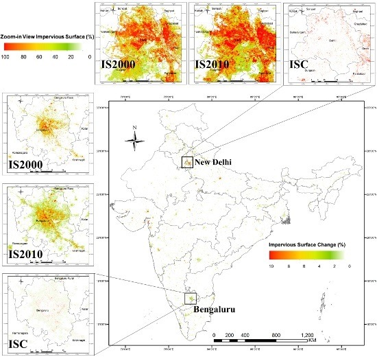
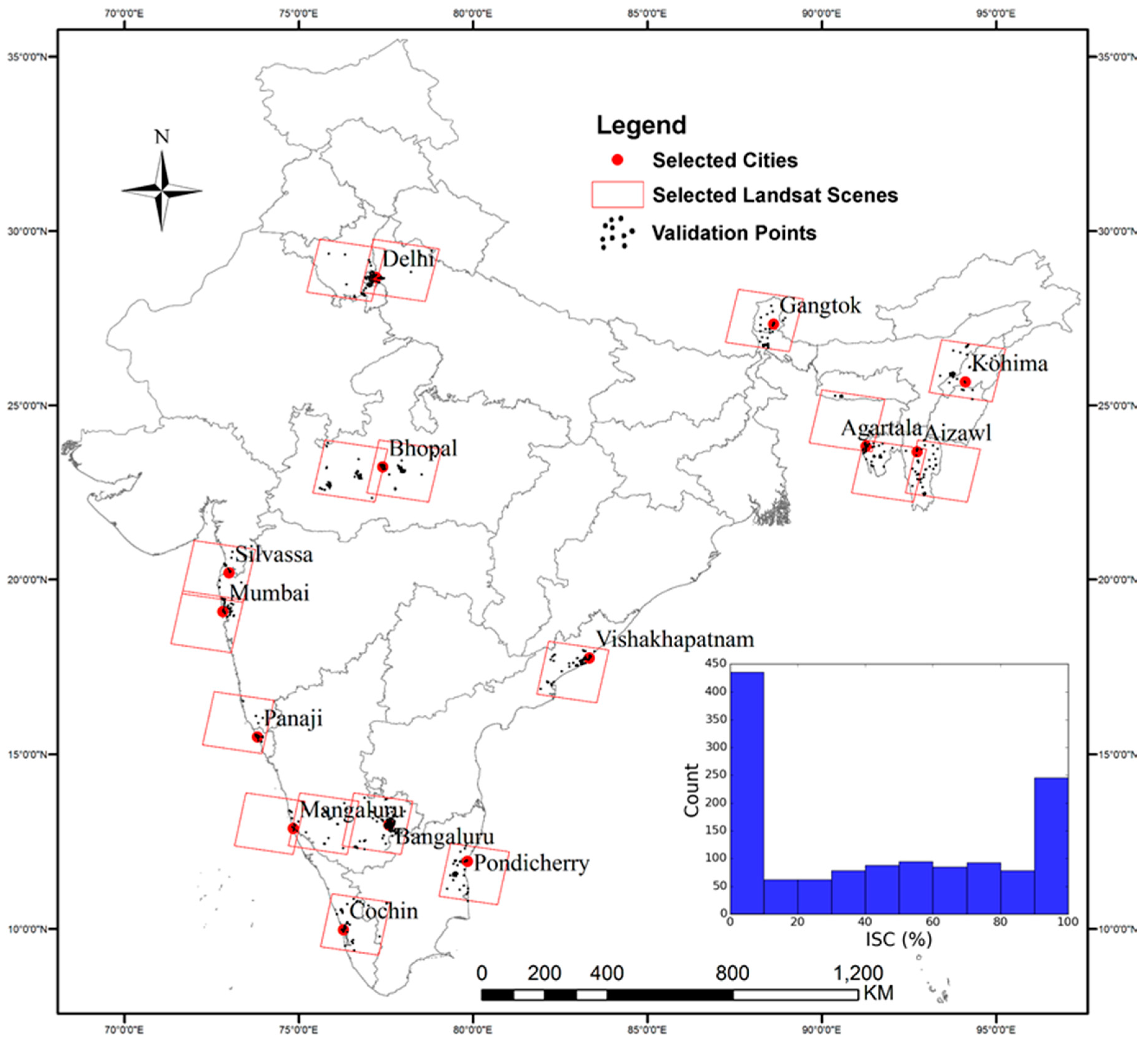
2.1. Study Area

The study area of this paper is India, a country with the seventh largest area (near 3.3 million km2) and second largest population (more than 1.2 billion as of 2016). India has gone through rapid urbanization for the first decade of the 21st century. From 2001 to 2011, India’s urban population has increased by 31.8%, much higher than its rural population growth rate of 12.2% [32,33]. With this alarming rate of urbanization, India faces many challenges. A previous study found that about 24% of the districts in India experienced significant agricultural land loss (>1000 hectare), which is mainly explained by urbanization [34]. Urbanization in India also has adverse impacts on biodiversity, as important habitats are being converted to impervious surface [35].
The issue of seasonal change in remotely sensed impervious surface is particularly severe in India. Because of the effect of monsoon and spatial distribution of rainfall, different vegetation dynamics spread across the country [36]. Also, shaped by the meteorological cycles, the spectral signatures of agricultural lands in India changes seasonally. For example, during dry months, fallow fields are often confused with impervious surfaces, which are difficult to separate with single temporal data [37].

2.2. Global Land Survey Surface Reflectance Datasets

Global Land Survey (GLS) datasets are global cloud-free collections of orthorectified Landsat images created by a collaborative effort of the US Geological Survey (USGS) and the National Aeronautics and Space Administration (NASA). Up to now, GLS datasets for the nominal years of 1975, 1990, 2000, 2005, and 2010 have been made available (Gutman et al. 2013). The GLS image selection procedures have produced image collections that meet data quality and cloud cover requirements for each epoch, which greatly reduced the difficulties for large-scale land use/land cover change (LCLUC) mapping. This study used GLS-2000 and GLS-2010 surface reflectance (SR) datasets processed using the Landsat Ecosystem Disturbance Adaptive Processing System (LEDAPS) (Masek et al. 2006) by the Global Land Cover Facility (GLCF) at University of Maryland. Assessments of GLS-SR datasets for 2000 and 2005 have also shown that GLS-SR has high agreement with MODIS SR and has satisfactory radiometric quality (Feng et al. 2013). To cover all the land areas of India, this study used 195 GLS Landsat scenes for each epoch.

2.3. Impervious Surface Mapping for 2010

A regression tree–based method was developed to map impervious surface (IS) for 2010. This study adopted a method similar to the NLCD impervious surface product using Landsat spectral bands as input variables and using IS percentage interpreted from high resolution images as training data. In addition to the six Landsat spectral bands, inputs to the regression tree model also included four spectral indices. These spectral indices were calculated as follows (Crist 1985; Kriegler et al. 1969):
B r i g h t n e s s = 0.2043 × b 1 + 0.4158 × b 2 + 0.5524 × b 3 + 0.5741 × b 4 + 0.3124 × b 5 + 0.2303 × b 7 ,
G r e e n e s s = 0.1603 × b 1 0.2819 × b 2 0.4934 × b 3 + 0.7940 × b 4 0.0002 × b 5 0.1446 × b 7 ,
W e t n e s s = 0.0315 × b 1 + 0.2021 × b 2 + 0.3102 × b 3 + 0.1594 × b 4 0.6806 × b 5 0.6109 × b 7 ,
N D V I = b 4 b 3 b 4 + b 3 ,
where b1~b7 are surface reflectance of Landsat TM/ETM bands.
The regression tree model was generated by the Cubist™ software by Rulequest, Empire Bay, Australia [38], a machine learning algorithm widely used for mapping IS as well as other continuous field land cover variables [25,29,30,39]. In addition to the predicted variable, Cubist™ also generates mean absolute error (MAE) estimations, which we have modified into root-mean-square error (RMSE) using a public version of Cubist™ code.
Due to spectral similarity between impervious surface and other non-impervious land cover types such as agricultural field and bare land, regression tree tends to overestimate impervious surface cover in these areas. Therefore, an urban mask is needed to mask out the impervious surface predictions out of the urban extent. Compared to the NLCD impervious surface product, which uses a nighttime light data set derived from DMSP-OLS [40], this study used object-based texture information to classify Landsat images into binary masks of human built-up and settlement extent (HBASE), which includes impervious and non-impervious surface covers within the urban boundary and smaller settlements such as towns and villages. The HBASE classification was performed using the Random Forest algorithm, an ensemble machine learning algorithm based on decision trees [41]. With Random Forest, this study generated not only the categorical classes for every pixel but also the probability of a pixel belonging to each class, which will be used later in this study (Section 2.4.3).
Training data for IS and HBASE machine learning models were collected throughout the globe for a global impervious surface mapping project. This paper used models based on training datasets developed for the Asian continent to map IS and HBASE in 2010. Initial assessments using cross validation estimated that the RMSE of IS to be 12.3% for the Asian IS model. For the Asian HBASE classification model, according to the result of cross validation, user’s accuracy, producers’ accuracy, overall accuracy, and kappa statistic were 91.5%, 90.3%, 97.9%, and 90.0%, respectively. More details on the methodologies used for 2010 IS and HBASE mapping will be provided in future papers.

2.4. Impervious Surface Mapping for 2000

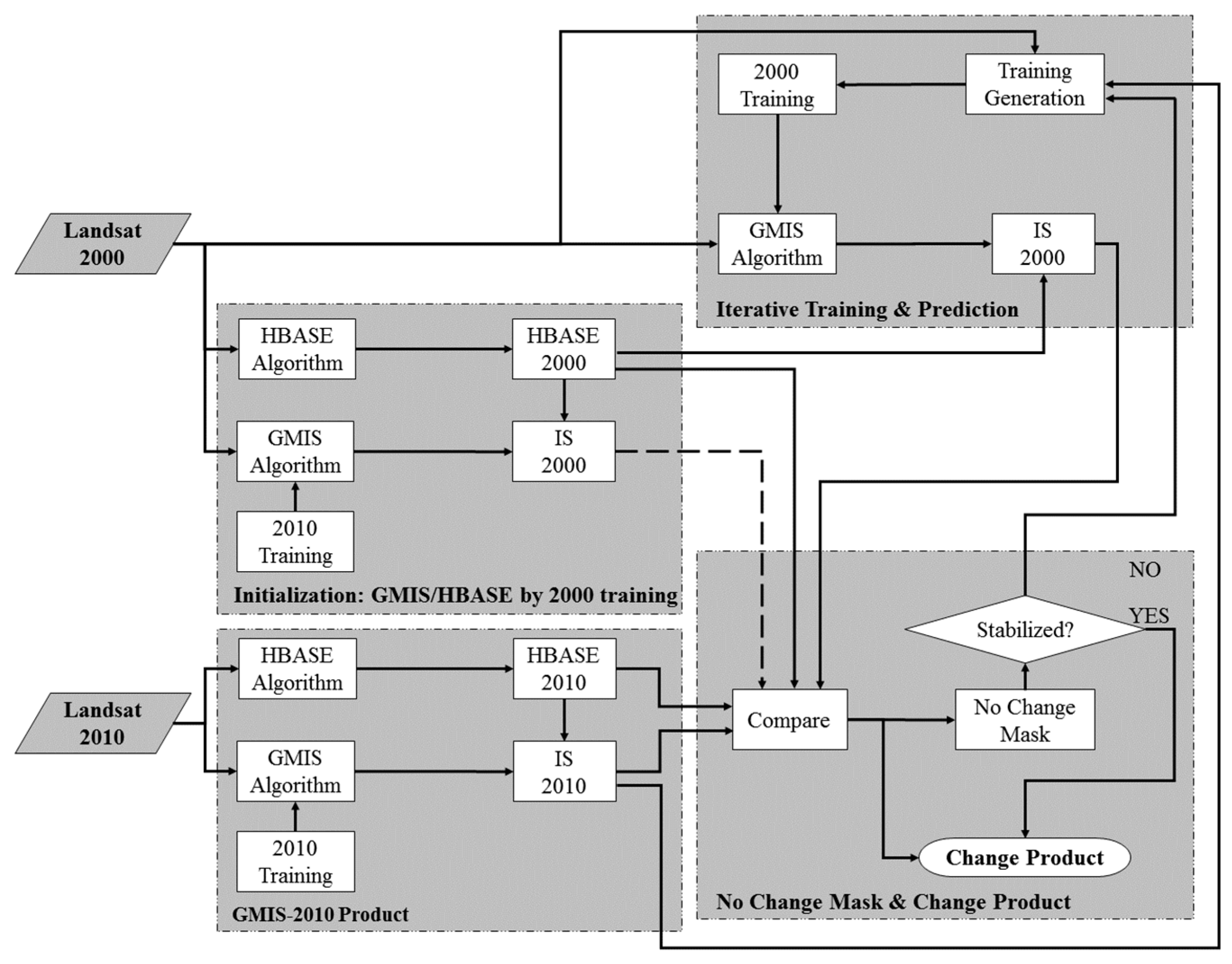
2.4.1. Overall Algorithm Design

Given the processing chain developed for mapping 2010 IS, the task of estimating ISC between 2000 and 2010 could be reduced to porting the 2010 IS model for mapping 2000 IS. Due to differences in acquisition dates and imaging geometries between corresponding GLS-2000 and GLS-2010 images, there are considerable spectral and phenological differences between images for these two epochs. As a result, the 2010 IS model could not be directly applied to GLS-2000. In order to produce high quality 2000 IS, the regression tree algorithm must be supplied with training data for the 2000 epoch. Instead of collecting training data for 2000, which cannot be achieved for many areas due to lack of necessary high resolution images, this study’s approach for estimating 2000 impervious surface cover was an iterative process designed to identify pixels whose IS values did not change between 2000 and 2010. Using the 2010 IS prediction for these pixels as training data, a regression tree was developed to map 2000 IS. The major steps of the overall methodology are shown as gray boxes in Figure 1. The following section will provide details on each one of these steps.

2.4.2. Algorithm Initialization

Initial estimation of IS-2000 was produced by simply applying the Cubist™ regression tree model used for 2010 IS mapping to the 2000 Landsat images. The 2010 HBASE classification model was also applied to 2000 Landsat data to produce 2000 HBASE maps. Since the HBASE algorithm is based on the classification of texture features, which were found to not be sensitive to spectral and phenological variations, this HBASE mapping result was used for all the subsequent analyses.

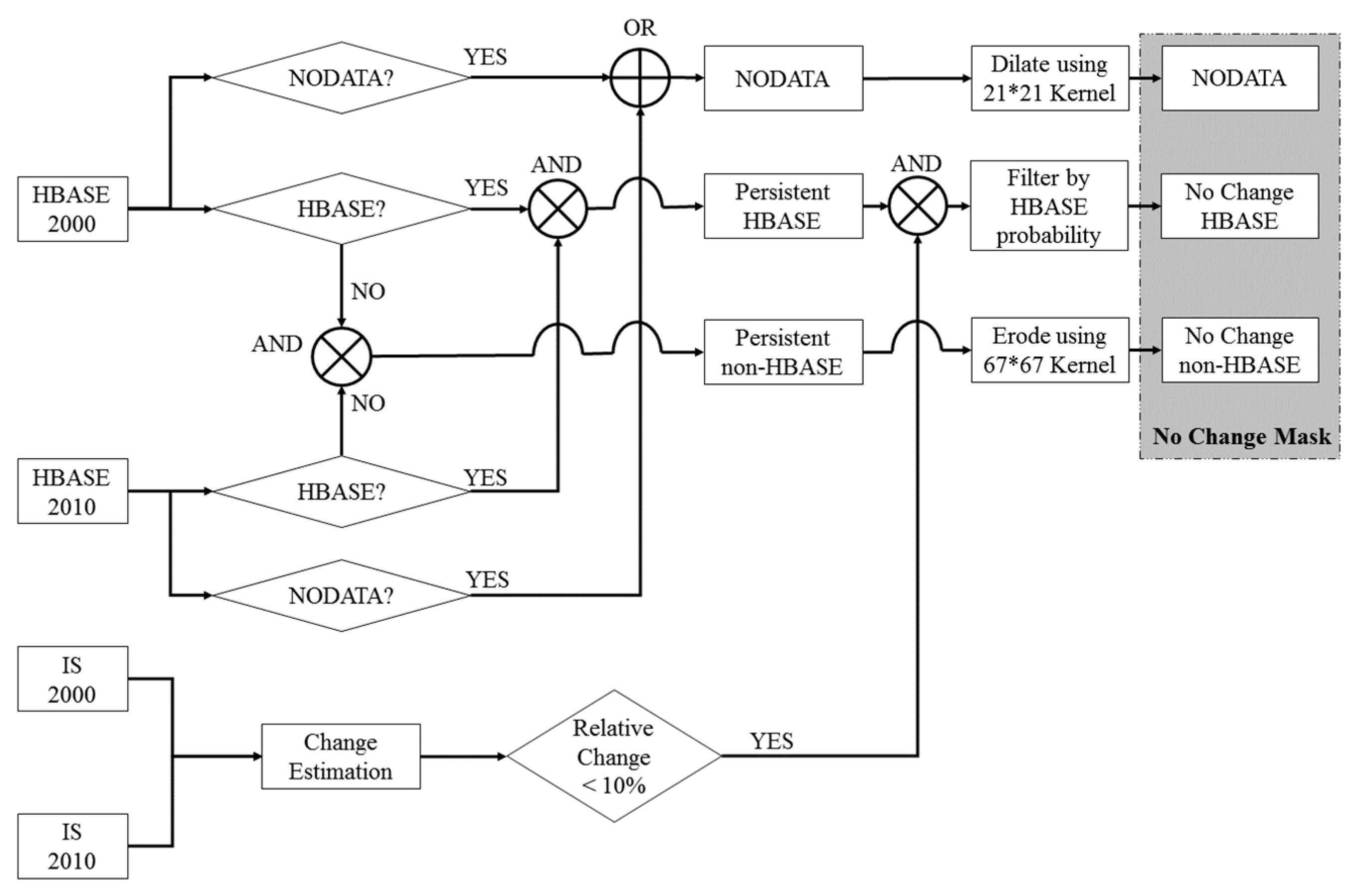
2.4.3. No Change Mask Generation

The goal of generating a “No Change” (NC) mask is to provide a set of pixels where IS-2000 could be considered equal to IS-2010 with great confidence. Since IS-2010 of these pixels will be used as training data for estimating IS-2000, the best information available and heuristics were used to get a conservative NC mask (meaning that NC mask is designed to include a minimum amount of change pixels). Figure 2 gives the criteria for determining if a pixel is in the NC mask.
First, pixels that were mapped were taken as non-HBASE for both 2000 and 2010 by the HBASE algorithm. These pixels could be considered as 0% impervious for both epochs. To further reduce commission error, an erosion morphological operator was applied using a 67 × 67 kernel, which generated a set of pixels with at least 1 km (33 Landsat pixels) distance to any HBASE pixels. The resulting pixels were labeled as “No Change non-HBASE” (NC-non-HBASE) in the NC mask.
Second, pixels were taken that were mapped as HBASE for both 2000 and 2010 by the HBASE algorithm. For these pixels, the relative impervious surface change between 2000 and 2010 was calculated as 2 × ( I S 2010 I S 2000 ) / ( I S 2010 + I S 2000 ) . Pixels with less than 10% relative change were considered to be “no change HBASE” (NC-HBASE). Since the HBASE classification may contain commission errors, the NC-HBASE category may contain non-HBASE pixels. Using of such pixels for training the 2000 model may lead to systematic bias the estimated 2000 impervious surface. To filter out remaining non-HBASE pixels, the class probability output of the HBASE classification model was leveraged and removed from the NC-HBASE category pixels where HBASE probability for either date is below a threshold. This study used 60% as the threshold for HBASE probability. This threshold, as well as the 10% threshold for relative change, was determined empirically based on accuracy of estimated ISC.
Finally, HBASE product contains “NODATA” pixels where there are clouds/shadows or data gaps as a result of the failure of Scan Line Corrector (SLC) of Landsat 7 [42]. A dilation morphological operator was applied using a 21 × 21 kernel to the “NODATA” pixels. This large buffer was designed to minimize potential impact of pixels adjacent to bad observations on the identification of NC pixels.

2.4.4. Iterative Training and Prediction (ITP)

Based on the NC mask, a training dataset was created for each GLS-2000 image: pixels within the NC-HBASE class were assumed to have impervious surface cover as predicted by the GMIS-2010 product; pixels within the NC-non-HBASE class were given 0% impervious surface cover. Using these training datasets, we trained Cubist™ regression tree models for each GLS-2000 image to predict 2000 impervious surface cover from Landsat data.
While it was assumed that the IS values of all NC-HBASE pixels did not change between 2000 and 2010, some of those pixels could have changes in their IS values. For example, redevelopment of an urban block could completely change the IS value of that block. Increasing building density in a low density urban area will result in substantial increase in the IS value. Such pixels should not be used as training pixels in developing the 2000 IS Cubist model. To identify such pixels, an iterative training and prediction (ITP) approach was adopted: the initial estimation of IS-2000 from regression tree model based on 2010 training data was denoted as 0-th iteration; for the k-th iteration, we generated a NC mask using IS-2000 from the (k − 1)-th iteration; the ITP process continued and generated a new IS-2000 based on the k-th NC mask until the k-th NC mask satisfies stabilization criterion
T 0 + T 1 T 0 + T 1 + T 2 × 100 % < 10 % ,
where T 0 is the number of pixels labelled as NC-HBASE for the (k − 1)-th NC mask but not the k-th NC mask, T 1 is the number of pixels labelled as NC-HBASE for the k-th NC mask but not the (k − 1)-th NC mask, and T 2 is the number of pixels labelled as NC-HBASE for both the k-th and the (k − 1)-th NC mask.
When the stabilization criterion was met, the NC mask was considered accurate enough and was used to generate the final IS-2000. HBASE-2000 from the algorithm initialization stage was used to filter out overestimation of IS in non-HBASE areas.

2.5. Quantification of 2000–2010 Impervious Surface Change

A simple subtraction of the final IS-2000 from the IS-2010 product was used to map the impervious surface change (ISC) between 2000 and 2010. In rapidly developing countries like India, most urban changes increase imperviousness. When the predicted IS-2010 is smaller the predicted IS-2000, it is much more likely due to natural factors such as changes in vegetation phenology instead of real decrease of imperviousness. Therefore, we set all the pixels with negative ISC to 0.
To further reduce noises in the ISC product, the RMSE output using the modified Cubist™ code was utilized. Under the assumption that IS2000 and IS2010 are independent, the standard error of an ISC prediction is estimated using
σ I S C R M S E I S 2000 2 + R M S E I S 2010 2 ,
where R M S E I S 2000 and R M S E I S 2010 the RMSE of 2000 and 2010 IS predictions estimated by the Cubist™ regression tree algorithm. We applied a threshold of one standard error to the ISC predictions, which was determined empirically to minimize the RMSE of estimated ISC. ISC predictions below one standard error were set zero.

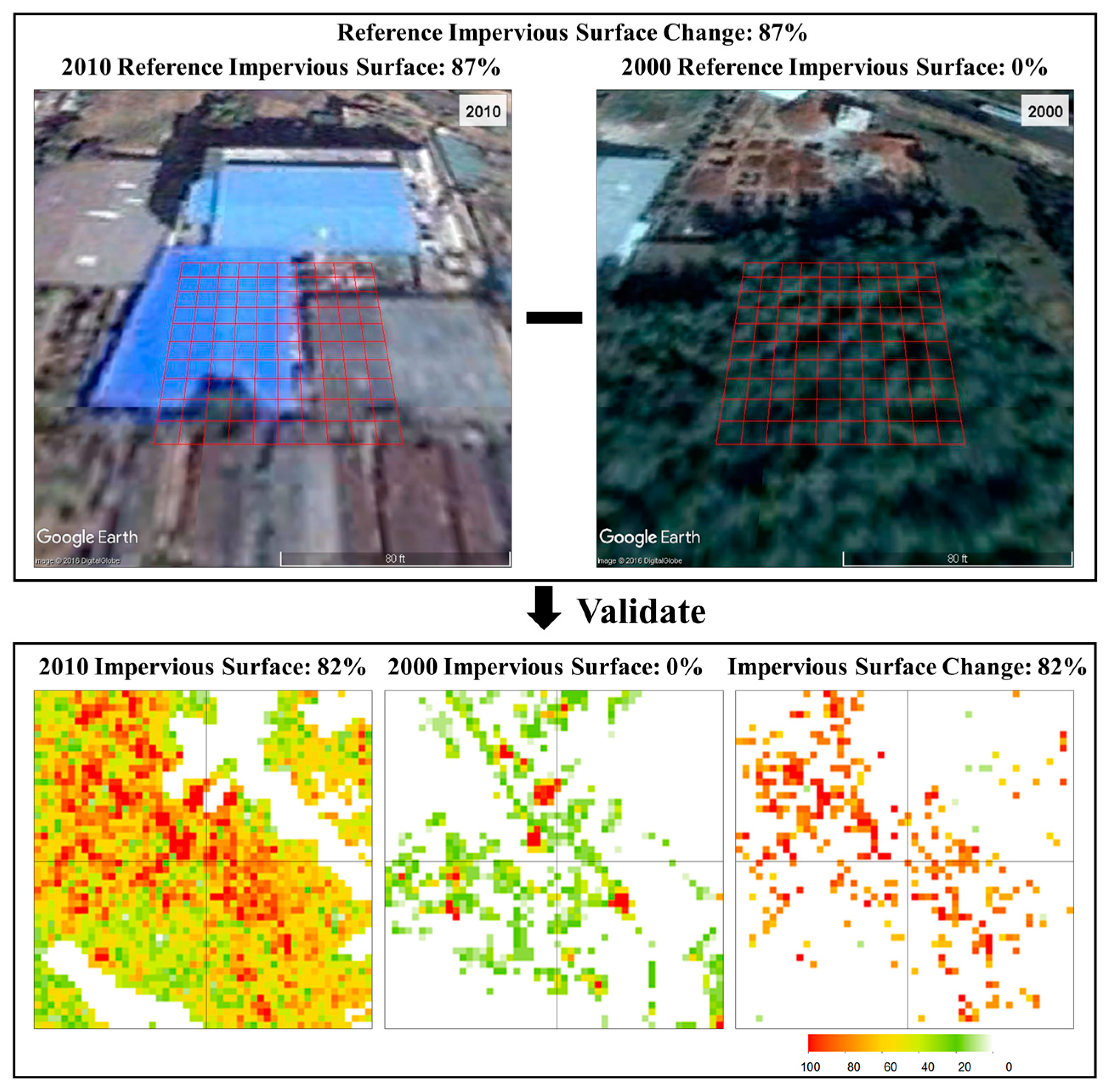
2.6. Validation of 2000–2010 Impervious Surface Change

In order to assess the accuracy of the produced ISC dataset, we developed an ISC validation dataset using Google Earth™ imagery, which uses pan-sharpened QuickBird imagery with 61 cm resolution and pan-sharpened Worldview-2 imagery with 46 cm resolution as sources of high resolution image for our study period. The selection of validation points followed a three-step stratified sampling approach:
  • The 500 most populous Indian cities were classified into seven groups: more than 5 million, 1~5 million, 500~1000 thousand, 250~500 thousand, 100~250 thousand, 50~100 thousand, and less than 50 thousand. From each group, two cities were selected. In total, 14 cities were selected that distribute across different regions of India;
  • Eighteen Landsat scene covering these 14 cities were identified;
  • For every Landsat scene, randomly select 50 pixels from each of these four groups:   I S C   =   0 , 0 < I S C 25 % ,   25 % < I S C 50 % ,   I S C > 50 % .
The authors then searched through the historical Google Earth™ imagery archive to find two images closest to the GLS-2000 and GLS-2010 acquisitions dates for each of the 3600 sample points. To be used as an ISC validation points, the following rules must be satisfied:
  • The difference between Google Earth™ and Landsat image acquisition dates is within two years (730 days) for both 2000 and 2010. This constrain could be relaxed if multiple Google Earth™ images with the same ISC were found before, during, and after the date range between GLS-2000 and GLS-2010;
  • There are no clouds/shadows in Google Earth™ image for both dates;
  • There are no apparent misregistration errors between two Google Earth™ images.
A Google Earth™ imagery interpretation tool was developed for estimating ISC (Figure 3). Using the rules listed above, it was determined that 1322 points, which is about 1/3 of the randomly sampled validation points, was interpretable. Among the 2278 dropped points, 1835 points were uninterpretable because of the first rule, and the rest were dropped because misregistration was found between Google Earth™ images for two dates. Although the randomness of samples may be compromised after filtering out the uninterpretable points, the validation dataset is still distributed across India and represents the entire range of ISC (Figure 4). For each of the usable validation points, the extent of the Landsat pixel was overlaid on 2000 and 2010 Google Earth™ images. The Landsat pixel to be validated was divided into 10-by-10 grids. By counting the number of grids with impervious surface cover, we estimated IS for 2000 and 2010. For example, in Figure 3, 87 out of 100 grids were covered by impervious surface in 2010 and no grid was covered by impervious surface in 2000. Therefore, it was estimated that IS 2010, IS 2000, and ISC were 87%, 0%, and 87%, respectively.

3. Results

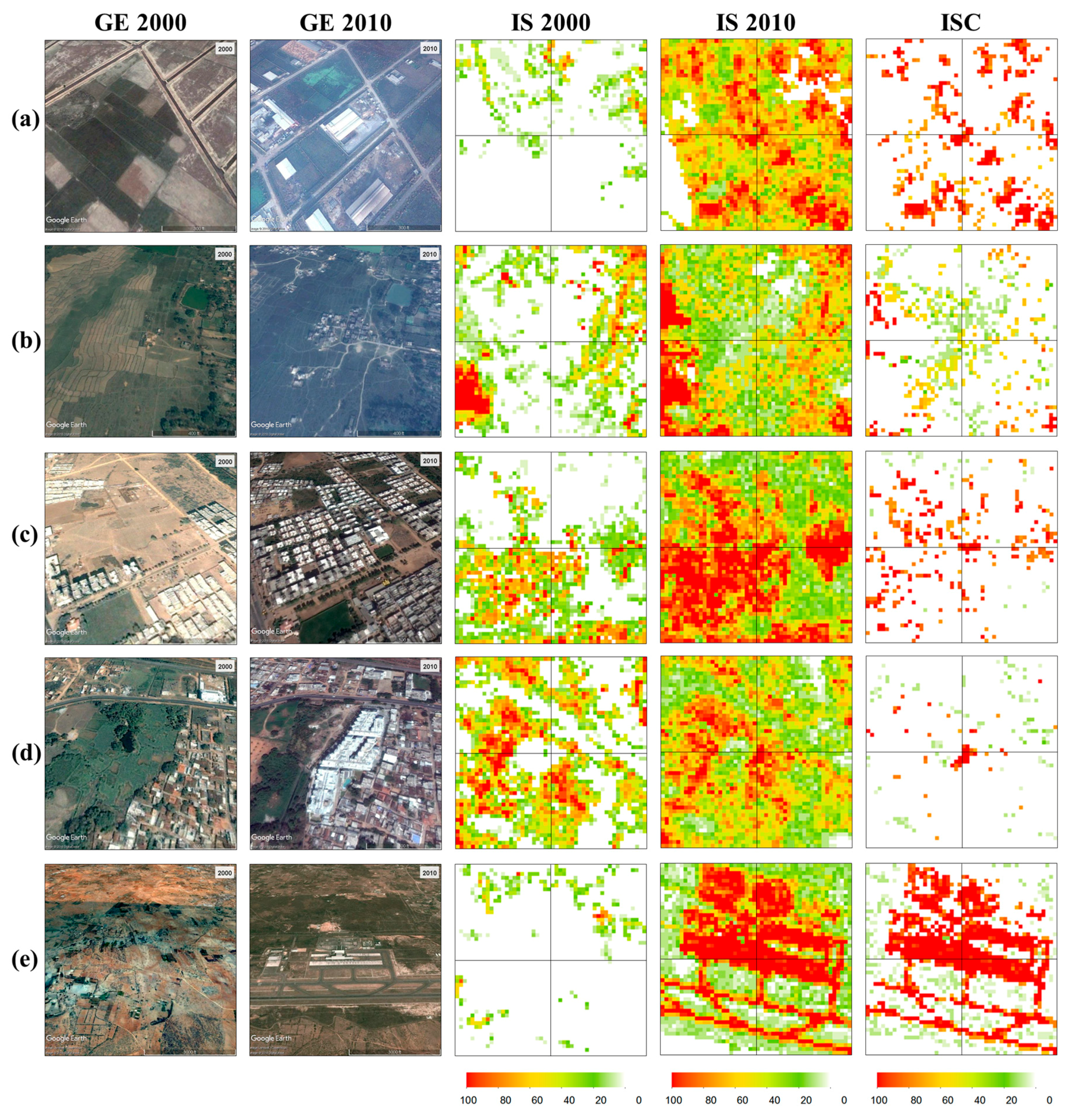
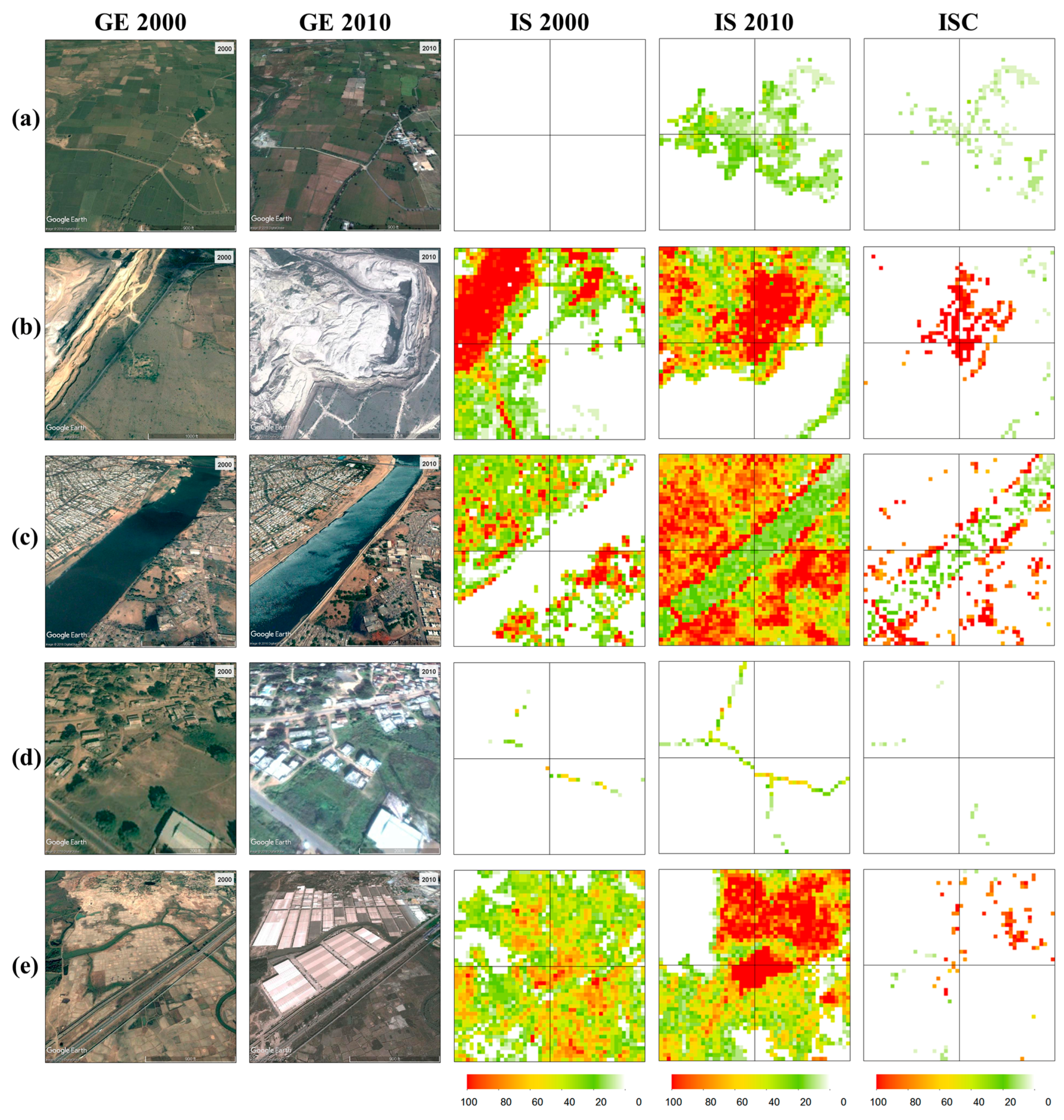
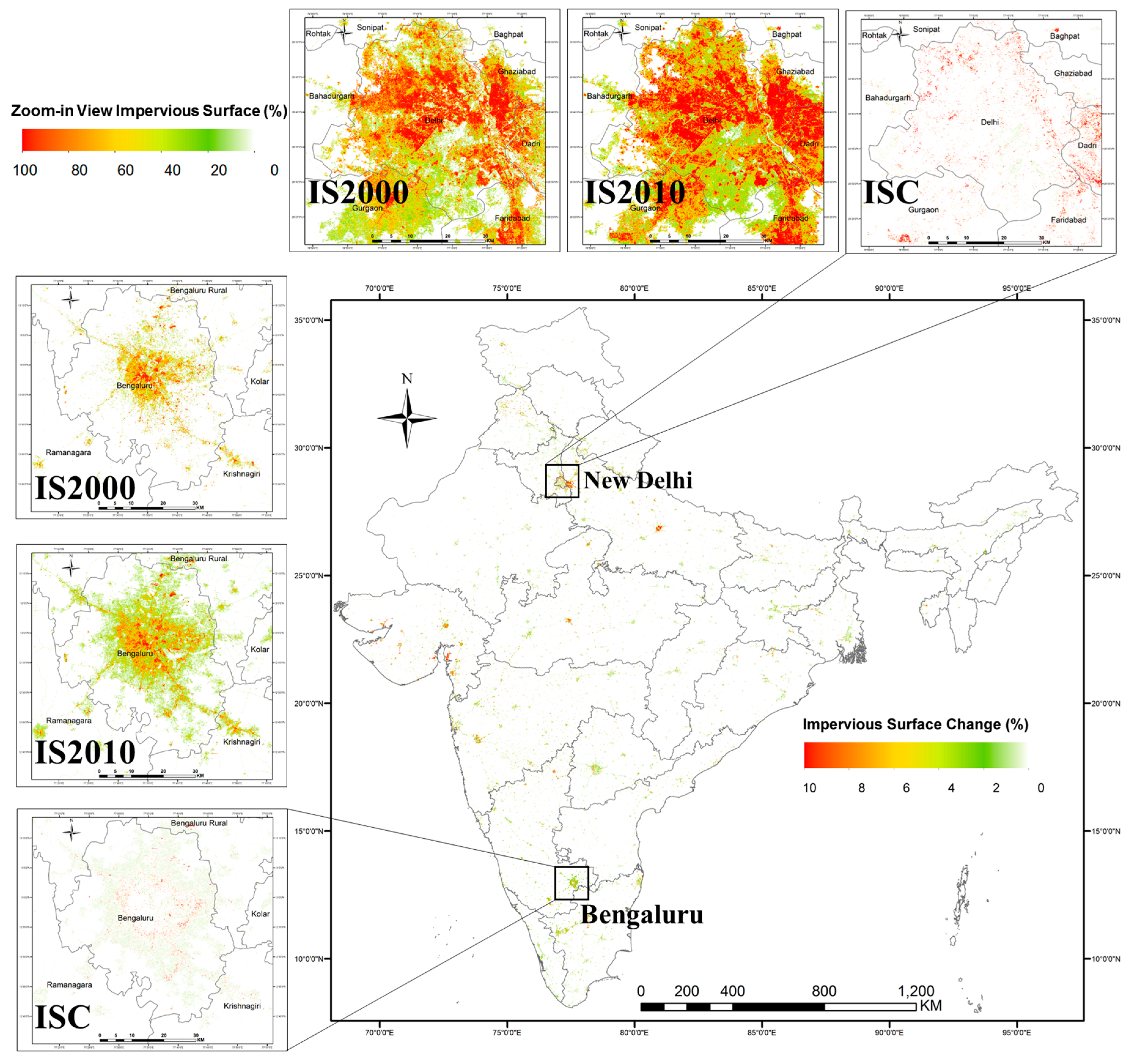
3.1. Visual Assessments of the IS and ISC Products

The quality of the bias-corrected ISC product was assessed first by visually examining it against Google Earth™ images. It was found that the ISC mapping method has good performance in different areas with a wide range of landscape characteristics and urban density. In Figure 5, site (a) is an area that was converted from agricultural field to high density impervious surface. 2000 IS mapped the center pixel as 0% correctly and 2010 IS mapped it as 95% impervious. Figure 5b shows an agricultural area converted to low to medium density impervious surface cover. The ISC product predicted a 44% increase of impervious surface cover. Figure 5c shows a bare area that started to be developed prior 2000 and continued converted to low to medium density impervious surface cover. The mapped ISC is 90%. Figure 5d shows a medium density area expanded with new high-rise residential buildings. Newly built areas were mapped as over 90% ISC. Figure 5e shows that a new airport was mapped correctly.
Although the overall performance is good, this study identified several types of errors in the IS and ISC products. In Figure 6a, an area remains agriculture land during the 2000–2010 period was mapped as low to medium density impervious surface cover for 2010, which resulted in a predicted ISC of 20%–40%. Mining areas are a major source of error, as shown in In Figure 6b. Both 2000 and 2010 have overestimated IS in this area. The expansion of mining caused an ISC prediction of over 90%. Turbulent water bodies were found to be confused with impervious surface. In Figure 6c, the river was correctly mapped as 0% impervious in 2000 but had around 20% IS retrievals in 2010. There are also cases when ISC is underestimated. Figure 6d shows a low density town undergoing intensification. But the IS products mapped only a few road pixels for both dates. This is caused by the omission error in the HBASE maps. Figure 6e shows an area where fallow agricultural fields are converted for industrial use. The 2010 IS product mapped the high impervious cover correctly. But since the IS 2000 product predicted medium IS with high standard error, the predicted change did not exceed one standard error and was set to zero.
A mosaic of the ISC product for the entire India was created to examine its overall spatial distribution pattern (Figure 7). First, the ISC changes are mainly distributed near existing urban clusters (e.g., New Delhi, Mumbai, and Bengaluru) where there has been strong population and economic growth during the 2000–2010 period. Second, Uttar Pradesh, Maharashtra, Gujarat, and Tamil Nadu are among the states with most ISC, which agrees with the MODIS-based analysis of agricultural land to urban land conversion in India [34]. Finally, as shown by the zoom-in views for New Delhi and Bengaluru, most of the impervious surface changes are in the urban fringe areas, which is an accurate representation of urban development patterns of these two cities.

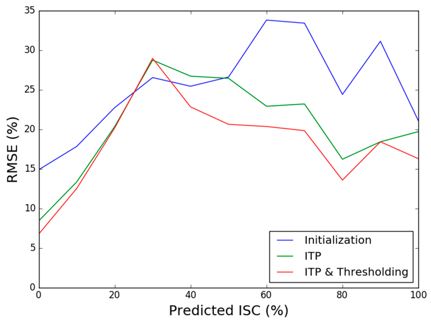
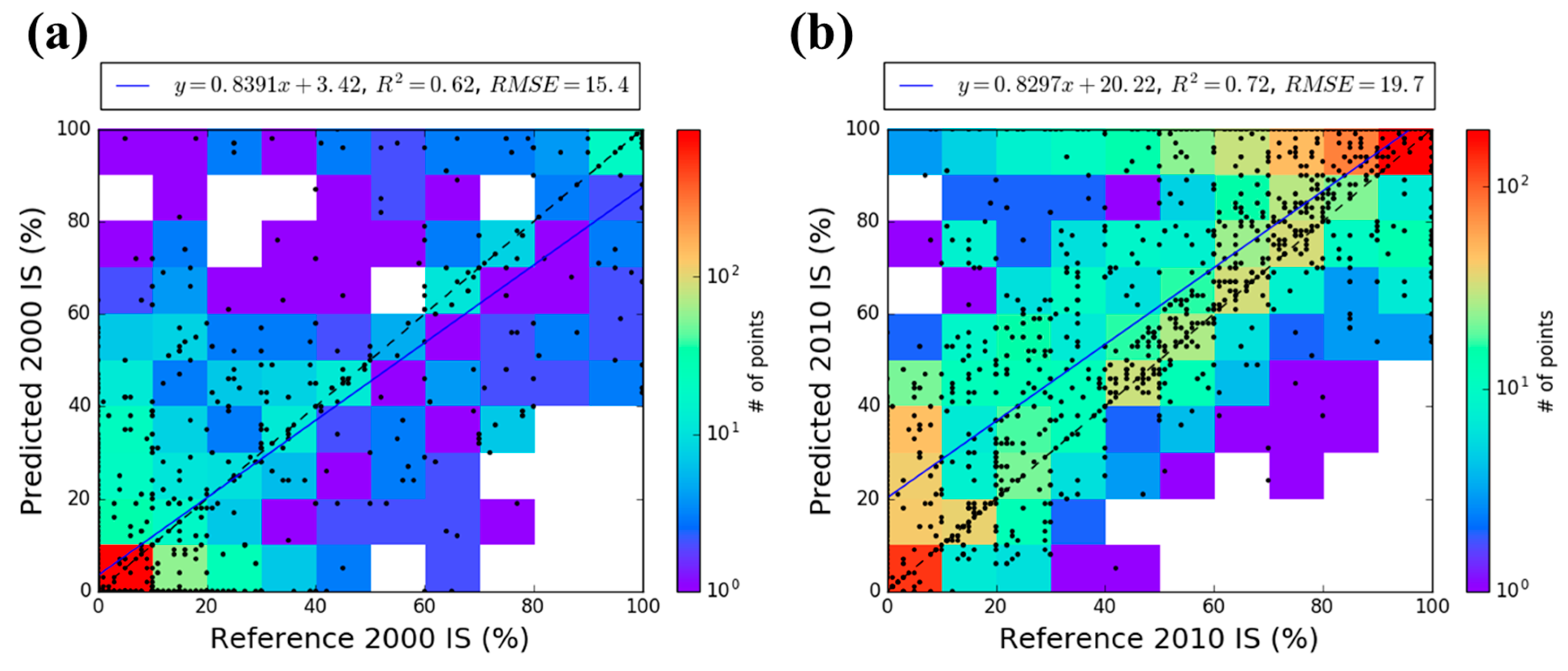
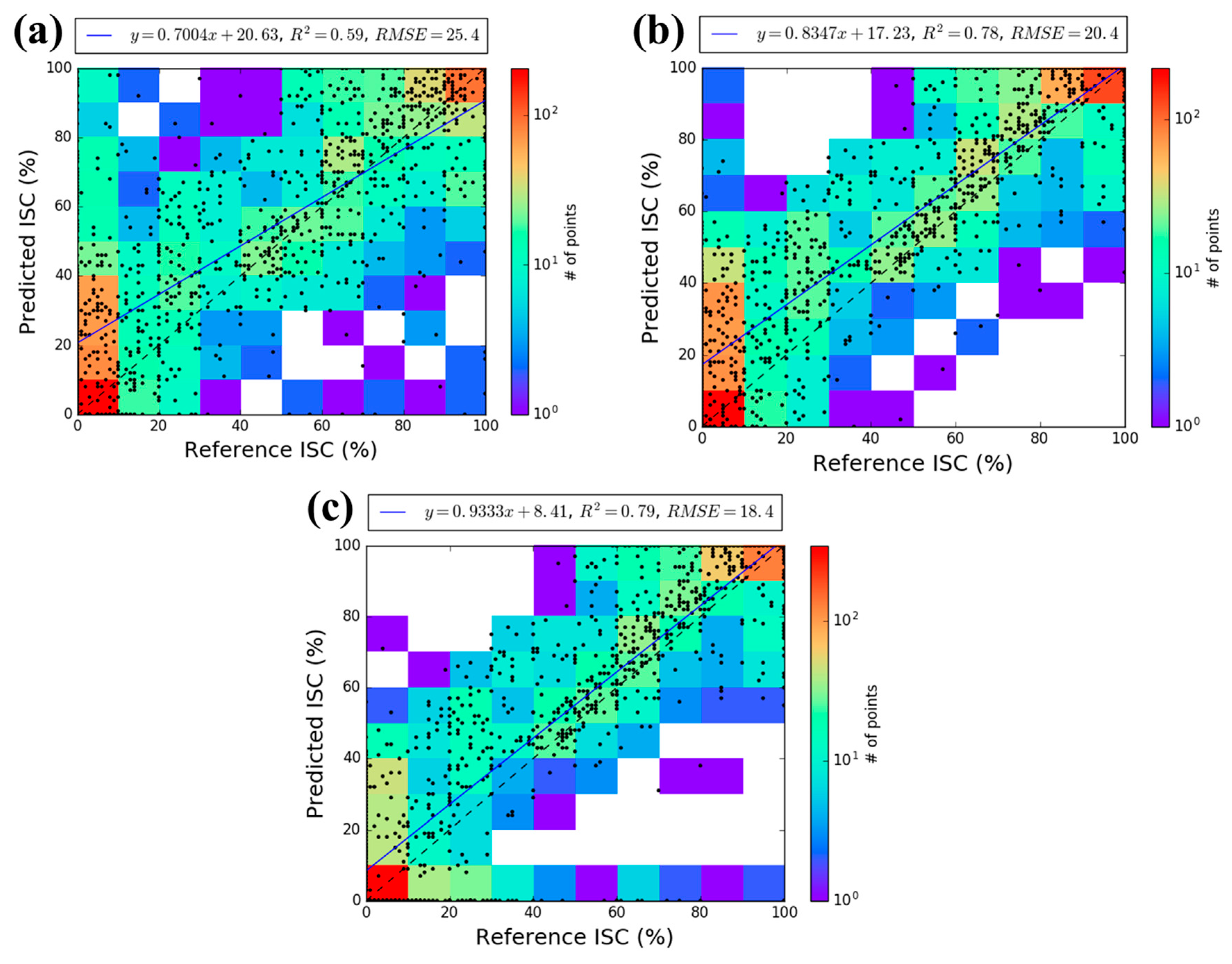
3.2. Accuracies of IS and ISC Products

The validation dataset developed in Section 2.6 was used for additional assessment of the IS and ISC products. Figure 8 shows the scatter plots between reference and predicted IS for 2000 and 2010. Colors were assigned to the scatterplot using numbers of points for each 10% by 10% grid. The RMSE of IS 2000 is 15.4% while the RMSE of IS 2010 is 19.7%. Figure 9 gives the scatter plots between reference and predicted ISC for the ISC result using IS-2000 from algorithm initialization in Section 2.4.2, ISC result after iterative training, and prediction (ITP) in Section 2.4.4 and final ISC product after applying the one standard error threshold. Figure 9a serves as a good example of the magnitude of errors in ISC when estimating IS using the same regression tree model for two dates. Without the ITP process, the RMSE of ISC was higher than the RMSE of IS for both epochs. After the ITP process, it is clear that the agreement between reference and predicted ISC improved significantly, which is demonstrated by the increase of R 2 from 0.59 to 0.78 and the decrease of RMSE from 25.4% to 20.4% in Figure 9b. Figure 9c shows that further improvement of accuracy was obtained by applying the one standard error threshold.
The statistical distribution of ISC values in the actual dataset might be significantly different from the histogram of reference ISC as shown in Figure 4. In order to better assess the errors of the ISC product. RMSE for each 10% predicted ISC intervals were estimated using the validation dataset (Figure 10), which established a lookup table between an ISC prediction and its corresponding RMSE estimation. This lookup table was used to assign a RMSE estimation for each pixel as the approximate standard deviation for the ISC prediction.

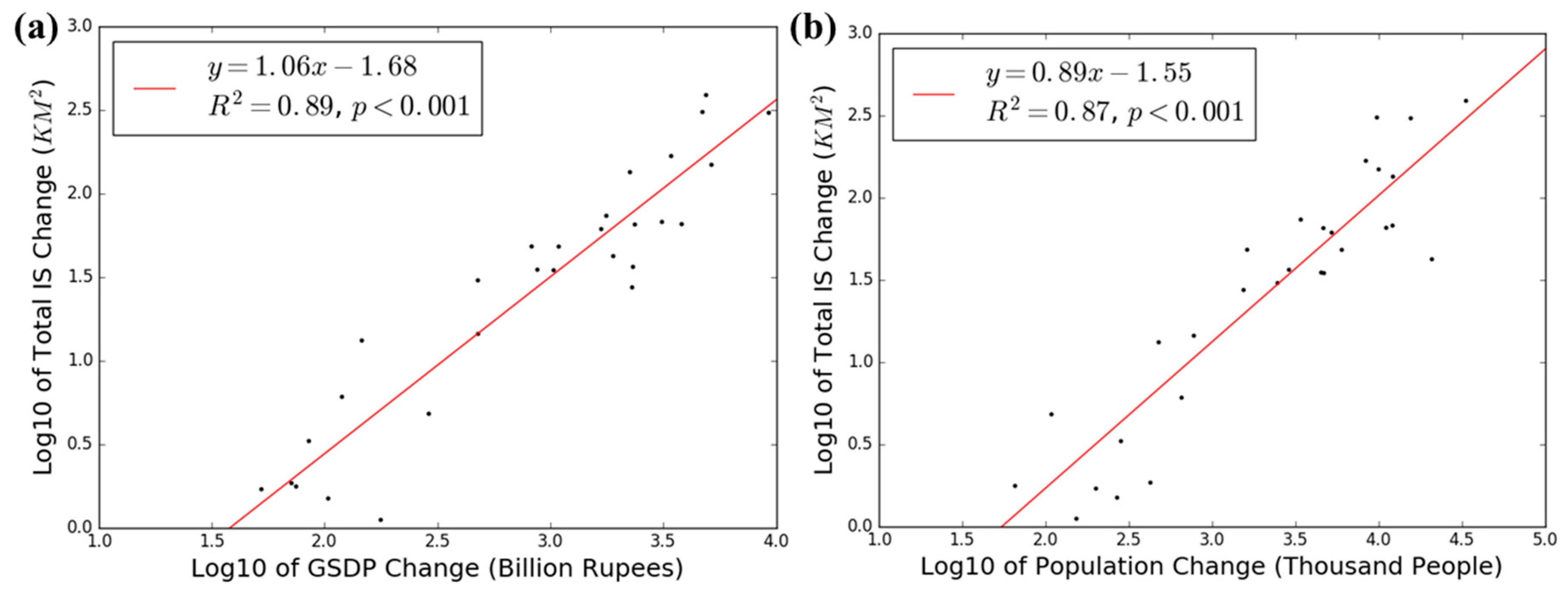
3.3. ISC in India and Relationships between ISC and Socio-Economic Change

For every state and union territory of India, impervious surface change area (ISCA) and its standard deviation (STD) were calculated by
I S C A = 0.0009 × i = 0 N I S C i   ,
σ I S C A 0.0009 × i = 0 n σ i 2 0.0009 × i = 0 n R M S E I S C i 2   ,
where I S C i is the predicted impervious surface change for the i-th pixel, N is the number of pixels within the state boundary, 0.0009 is the size of a Landsat pixel in km2,   σ I S C A is the standard deviation of ISCA for the state, and σ i is the standard deviation of ISC for the i-th pixel, which is approximated using the estimated RMSE for the impervious surface change, under the assumption that there is no spatial autocorrelation in the estimated ISC. The ISCA calculation was based on state boundaries defined by the Global Administrative Areas (GADM) dataset [43].
Population growth and economic development are known as two major drivers of urbanization. To examine the relationship between the mapped ISC and socio-economic change in India, state-wise change statistics were also calculated for gross state domestic product (GSDP) and population between 2001 and 2011 (see Figure 11). The GSDP data was released by Planning Commission of India [44], and the population data was retrieved from India Census 2001 and 2011 [32]. These statistics are listed in Table 1. GSDP and population data for three small union territories (Dadra and Nagar Haveli, Daman and Diu, and Lakshadweep) were not available. Also, the GADM state boundaries have Andhra Pradesh and Telangana as two different states, which were separated from the state of Andhra in 2014. At the time when GSDP and population data were collected, these two states were not yet separated; therefore, this study did not calculate GSDP and population change for them.
The state-wise total impervious surface change are plotted in Figure 10 against (a) gross state domestic product (GSDP) change and (b) population change from Table 1. Both GSDP and population have good correlations with the ISC product.

4. Discussion

This approach for ISC mapping is designed to solve the fundamental problem of estimating ISC from bi-temporal images using spectral information, which is the sensitivity of estimated impervious surface to spectral and phenological differences between bi-temporal images. Instead of applying an existing year 2010 regression tree to GLS-2000 images, this study designed an iterative training and prediction (ITP) process to automatically generate training data for a year 2000 regression tree model, estimated IS-2000, and mapped ISC as the difference between IS-2010 and IS-2000.
As shown by visual assessments, quantitative assessments using an independent validation dataset, and the correlation between ISC and changes in population and GDP, this ISC mapping algorithm achieved a high level of accuracy. However, the final ISC products still shows a bias towards overestimation as a result of underestimated 2000 IS (see Figure 8a) and overestimated 2010 IS (see Figure 8b). Several methodological limitations and sources of errors remains to be better addressed in future studies.
First, the generation of NC mask and subsequently the training datasets for 2000 relies on HBASE masks. If an impervious pixel is classified as non-HBASE for both 2000 and 2010, it might be included in the 2000 training as 0% impervious. Inclusion of such pixels in 2000 training could lead to underestimation of IS-2000 and therefore overestimation of ISC. To better identify pixels without impervious surface change, unsupervised change detection methods and spectral mixture analysis may yield better results than the heuristic method used in this study.
Second, regression trees are known to have tendency of overestimation in non-impervious areas spectrally similar to impervious surface [23,27]. This study used HBASE masks to remove retrievals of impervious surface in these areas. Yet there are commission errors in the HBASE masks as shown by Figure 6a, where ISC might be overestimated. Also, HBASE masks have omissions errors in low to medium density villages/towns, where ISC might be underestimated. These issues highlight the importance of an accurate HBASE/urban mask for ISC estimation. Other currently available global urban maps may be used in addition to or as an alternative to the HBASE product used in this study. These maps include the GlobeLand30 product (30 m) [20], the MODIS Land Cover product (500 m) [14,45], and the map from the Global Rural Urban Mapping Project (GRUMP) [16]. More studies on better representation of HBASE/urban in global maps could lead to better estimation of ISC under the presented framework.
Third, by applying the one standard error threshold to ISC predictions, the overestimation of ISC in areas where IS is overestimated were reduced. The RMSE of the final ISC product is lower than the RMSE of 2000 IS or 2010 IS. However, this also introduced omission of real ISC in areas where the uncertainty of Cubist™ prediction were high. Bias correction methods as described in [46] might be a better way to remove bias when a high quality reference dataset is available.
Finally, the ITP process requires a large number of iterations to generate a stable NC mask and corresponding IS-2000. In processing the 195 Landsat scenes covering India, 152 scenes (78%) took more than 100 iterations to finish. More studies are needed to improve the computational efficiency of our algorithm for large-scale applications.
Addressing the problems above requires major methodological improvements. On the other hand, Landsat time series have been demonstrated to be able to deal with ISC errors associated with spectral and phenological differences in bi-temporal datasets [30]. Given the increasing availability of 30-m or finer resolution satellite datasets, including those acquired by Landsat 8 and Sentinel-2, ISC mapping using dense time series Landsat-like data could be done at large-scale in the near future.
Nevertheless, the method presented here shows great potential for large-scale ISC mapping. It could be particularly useful when mapping change between a recent date with good coverage of high resolution image and a much earlier date when high resolution data was scarce.

5. Conclusions

An iterative training and prediction (ITP) approach was developed for mapping impervious surface change (ISC). 2010 impervious surface was mapped using the well-established regression tree based method. Without additional training data collected for the 2000 epoch, 2000 impervious surface was mapped by automatically generated 2000 training data based on a “no change” (NC) mask. The estimated 2000 impervious surface was in turn used for generating a better NC mask in an iterative fashion.
The ITP method was applied to GLS Landsat images to produce a 2000–2010 ISC product for India. This product had a RMSE of 18.4% when evaluated using a validation dataset derived using Google Earth™ images. By calculating RMSE for every 10% intervals of the predicted ISC, we also found that RMSE for all the predicted ISC intervals were within the 5%–30% range. It is estimated that, if there is no spatial autocorrelation in the estimated ISC, at 95% confidence, the total ISC for India between 2000 and 2010 is 2274.62 ± 7.84 km2.
This study demonstrated the effectiveness of the ITP approach for mapping ISC consistently at national scales with a dataset that exhibited spectral differences between two dates. Such spectral differences may be attributed to differences in acquisition dates, illumination and viewing geometry, and vegetation phenology. With the ability to handle spectral inconsistency, the ITP approach may be useful for continuous field products for other major land cover types after minor adjustments.

Acknowledgments

This study was supported by NASA’s Land Cover and Land Use Change (LCLUC) Program (grants 09-LCLUC09-2-0136-1 & NNX11AH67G). Additional support for Panshi Wang and Chengquan Huang was provided by NOAA and the US Geological Survey. The authors thank Zhaoxin Li for her help in deriving the impervious surface change validation dataset that was used for product assessment. The authors would also like to thank Global Land Cover Facility at University of Maryland for providing the GLS-2000 and GLS-2010 surface reflectance dataset.

Author Contributions

Panshi Wang conceived and designed the study, developed computer programs for data processing and statistical analysis, and wrote the paper. Chengquan Huang and Eric Brown de Colstoun advised on the methodology, contributed ideas for the manuscript, and provided comments on a draft manuscript.

Conflicts of Interest

The authors declare no conflict of interest. The founding sponsors had no role in the design of the study; in the collection, analyses, or interpretation of data; in the writing of the manuscript; or in the decision to publish the results.

References

  1. United Nations. Department of Economic and Social Affairs, Population Division (2015); World Urbanization Prospects: New York, NY, USA, 2015. [Google Scholar]
  2. Arnfield, A.J. Two decades of urban climate research: A review of turbulence, exchanges of energy and water, and the urban heat island. Int. J. Climatol. 2003, 23, 1–26. [Google Scholar] [CrossRef]
  3. Seto, K.C.; Shepherd, J.M. Global urban land-use trends and climate impacts. Curr. Opin. Environ. Sustain. 2009, 1, 89–95. [Google Scholar] [CrossRef]
  4. Arnold, C.L.; Gibbons, C.J. Impervious surface coverage: The emergence of a key environmental indicator. J. Am. Plan. Assoc. 1996, 62, 243–258. [Google Scholar] [CrossRef]
  5. Foley, J.A.; Defries, R.; Asner, G.P.; Barford, C.; Bonan, G.; Carpenter, S.R.; Chapin, F.S.; Coe, M.T.; Daily, G.C.; Gibbs, H.K.; et al. Global consequences of land use. Science 2005, 309, 570–574. [Google Scholar] [CrossRef] [PubMed]
  6. Kaye, J.P.; Groffman, P.M.; Grimm, N.B.; Baker, L.A.; Pouyat, R.V. A distinct urban biogeochemistry? Trends Ecol. Evol. 2006, 21, 192–199. [Google Scholar] [CrossRef] [PubMed]
  7. Lambin, E.F.; Turner, B.L.; Geist, H.J.; Agbola, S.B.; Angelsen, A.; Bruce, J.W.; Coomes, O.T.; Dirzo, R.; Fischer, G.; Folke, C.; et al. The causes of land-use and land-cover change: Moving beyond the myths. Glob. Environ. Chang. 2001, 11, 261–269. [Google Scholar] [CrossRef]
  8. Liu, Z.; He, C.; Zhou, Y.; Wu, J. How much of the world’s land has been urbanized, really? A hierarchical framework for avoiding confusion. Landsc. Ecol. 2014, 29, 763–771. [Google Scholar] [CrossRef]
  9. Schneider, A.; Friedl, M.A.; Potere, D. A new map of global urban extent from modis satellite data. Environ. Res. Lett. 2009, 4, 044003. [Google Scholar] [CrossRef]
  10. Small, C. Global population distribution and urban land use in geophysical parameter space. Earth Interact. 2004, 8, 1–18. [Google Scholar] [CrossRef]
  11. Lambin, E.F.; Geist, H.J.; Lepers, E. Dynamics of land-use and land-cover change in tropical regions. Annu. Rev. Environ. Resour. 2003, 28, 205–241. [Google Scholar] [CrossRef]
  12. Lambin, E.F.; Meyfroidt, P. Land use transitions: Socio-ecological feedback versus socio-economic change. Land Use Policy 2010, 27, 108–118. [Google Scholar] [CrossRef]
  13. Hansen, M.C.; Defries, R.S.; Townshend, J.R.G.; Sohlberg, R. Global land cover classification at 1 km spatial resolution using a classification tree approach. Int. J. Remote Sens. 2000, 21, 1331–1364. [Google Scholar] [CrossRef]
  14. Friedl, M.A.; Sulla-Menashe, D.; Tan, B.; Schneider, A.; Ramankutty, N.; Sibley, A.; Huang, X. Modis collection 5 global land cover: Algorithm refinements and characterization of new datasets. Remote Sens. Environ. 2010, 114, 168–182. [Google Scholar] [CrossRef]
  15. Loveland, T.R.; Belward, A.S. The igbp-dis global 1 km land cover data set, discover: First results. Int. J. Remote Sens. 1997, 18, 3291–3295. [Google Scholar] [CrossRef]
  16. CIESIN (Center for International Earth Science Information Network). Global Rural-Urban Mapping Project, Version 1 (grumpv1): Urban Extents. 2011. Available online: http://sedac.ciesin.columbia.edu/data/collection/grump-v1 (accessed on 15 May 2016).
  17. Zhou, Y.; Smith, S.J.; Zhao, K.; Imhoff, M.; Thomson, A.; Bond-Lamberty, B.; Asrar, G.R.; Zhang, X.; He, C.; Elvidge, C.D. A global map of urban extent from nightlights. Environ. Res. Lett. 2015, 10, 054011. [Google Scholar] [CrossRef]
  18. Elvidge, C.D.; Tuttle, B.T.; Sutton, P.C.; Baugh, K.E.; Howard, A.T.; Milesi, C.; Bhaduri, B.; Nemani, R. Global distribution and density of constructed impervious surfaces. Sensors 2007, 7, 1962–1979. [Google Scholar] [CrossRef]
  19. Gong, P.; Wang, J.; Yu, L.; Zhao, Y.; Zhao, Y.; Liang, L.; Niu, Z.; Huang, X.; Fu, H.; Liu, S.; et al. Finer resolution observation and monitoring of global land cover: First mapping results with landsat tm and etm+ data. Int. J. Remote Sens. 2013, 34, 2607–2654. [Google Scholar] [CrossRef]
  20. Chen, J.; Chen, J.; Liao, A.; Cao, X.; Chen, L.; Chen, X.; He, C.; Han, G.; Peng, S.; Lu, M.; et al. Global land cover mapping at 30 m resolution: A pok-based operational approach. ISPRS J. Photogramm. Remote Sens. 2015, 103, 7–27. [Google Scholar] [CrossRef]
  21. Jensen, J.R.; Cowen, D.C. Remote sensing of urban suburban infrastructure and socio-economic attributes. Photogramm. Eng. Remote Sens. 1999, 65, 611–622. [Google Scholar]
  22. Yang, L.M.; Huang, C.; Homer, C.G.; Wylie, B.K.; Coan, M.J. An approach for mapping large-area impervious surfaces: Synergistic use of landsat-7 etm+ and high spatial resolution imagery. Can. J. Remote Sens. 2003, 29, 230–240. [Google Scholar] [CrossRef]
  23. Lu, D.S.; Li, G.Y.; Kuang, W.H.; Moran, E. Methods to extract impervious surface areas from satellite images. Int. J. Digit. Earth 2014, 7, 93–112. [Google Scholar] [CrossRef]
  24. Weng, Q.; Hu, X.; Lu, D. Extracting impervious surfaces from medium spatial resolution multispectral and hyperspectral imagery: A comparison. Int. J. Remote Sens. 2008, 29, 3209–3232. [Google Scholar] [CrossRef]
  25. Walton, J.T. Subpixel urban land cover estimation: Comparing cubist, random forests, and support vector regression. Photogramm. Eng. Remote Sens. 2008, 74, 1213–1222. [Google Scholar] [CrossRef]
  26. Xian, G.; Homer, C. Updating the 2001 national land cover database impervious surface products to 2006 using landsat imagery change detection methods. Remote Sens. Environ. 2010, 114, 1676–1686. [Google Scholar] [CrossRef]
  27. Yuan, F.; Wu, C.S.; Bauer, M.E. Comparison of spectral analysis techniques for impervious surface estimation using landsat imagery. Photogramm. Eng. Remote Sens. 2008, 74, 1045–1055. [Google Scholar] [CrossRef]
  28. Wu, C.S.; Yuan, F. Seasonal sensitivity analysis of impervious surface estimation with satellite imagery. Photogramm. Eng. Remote Sens. 2007, 73, 1393–1401. [Google Scholar] [CrossRef]
  29. Sexton, J.O.; Song, X.-P.; Huang, C.; Channan, S.; Baker, M.E.; Townshend, J.R. Urban growth of the washington, D.C.-baltimore, md metropolitan region from 1984 to 2010 by annual, landsat-based estimates of impervious cover. Remote Sens. Environ. 2013, 129, 42–53. [Google Scholar] [CrossRef]
  30. Song, X.-P.; Sexton, J.O.; Huang, C.; Channan, S.; Townshend, J.R. Characterizing the magnitude, timing and duration of urban growth from time series of landsat-based estimates of impervious cover. Remote Sens. Environ. 2016, 175, 1–13. [Google Scholar] [CrossRef]
  31. Swerts, E.; Pumain, D.; Denis, E. The future of india’s urbanization. Futures 2014, 56, 43–52. [Google Scholar] [CrossRef]
  32. Office of the Registrar General & Census Commissioner of Inida. Provisional Population Totals Paper 2 of 2011. 2011. Available online: http://www.censusindia.gov.in/2011-prov-results/paper2/census2011_paper2.html (accessed on 20 November 2016).
  33. Pandey, B.; Joshi, P.K.; Seto, K.C. Monitoring urbanization dynamics in india using dmsp/ols night time lights and spot-vgt data. Int. J. Appl. Earth Obs. Geoinf. 2013, 23, 49–61. [Google Scholar] [CrossRef]
  34. Pandey, B.; Seto, K.C. Urbanization and agricultural land loss in india: Comparing satellite estimates with census data. J. Environ. Manag. 2015, 148, 53–66. [Google Scholar] [CrossRef] [PubMed]
  35. Nagendra, H.; Sudhira, H.S.; Katti, M.; Schewenius, M. Sub-regional assessment of india: Effects of urbanization on land use, biodiversity and ecosystem services. In Urbanization, Biodiversity and Ecosystem Services: Challenges and Opportunities: A Global Assessment; Elmqvist, T., Fragkias, M., Goodness, J., Güneralp, B., Marcotullio, P.J., McDonald, R.I., Parnell, S., Schewenius, M., Sendstad, M., Seto, K.C., et al., Eds.; Springer: Dordrecht, The Netherlands, 2013; pp. 65–74. [Google Scholar]
  36. Tian, H.Q.; Banger, K.; Bo, T.; Dadhwal, V.K. History of land use in india during 1880–2010: Large-scale land transformations reconstructed from satellite data and historical archives. Glob. Planet. Chang. 2014, 121, 78–88. [Google Scholar] [CrossRef]
  37. Haack, B.N.; Solomon, E.K.; Bechdol, M.A.; Herold, N.D. Radar and optical data comparison/integration for urban delineation: A case study. Photogramm. Eng. Remote Sens. 2002, 68, 1289–1296. [Google Scholar]
  38. Rulequest Research Data Mining with Cubist. 2016. Available online: https://www.rulequest.com/cubist-info.html (accessed on 16 December 2016).
  39. Sexton, J.O.; Song, X.-P.; Feng, M.; Noojipady, P.; Anand, A.; Huang, C.; Kim, D.-H.; Collins, K.M.; Channan, S.; DiMiceli, C.; et al. Global, 30-m resolution continuous fields of tree cover: Landsat-based rescaling of modis vegetation continuous fields with lidar-based estimates of error. Int. J. Digit. Earth 2013, 6, 427–448. [Google Scholar] [CrossRef]
  40. Xian, G.; Homer, C.; Demitz, J.; Fry, J.; Hossain, N.; Wickham, J. Change of impervious surface area between 2001 and 2006 in the conterminous united states. Photogramm. Eng. Remote Sens. 2011, 77, 758–762. [Google Scholar]
  41. Breiman, L. Random forests. Mach. Learn. 2001, 45, 5–32. [Google Scholar] [CrossRef]
  42. Gutman, G.; Huang, C.; Chander, G.; Noojipady, P.; Masek, J.G. Assessment of the NASA–USGS global land survey (GLS) datasets. Remote Sens. Environ. 2013, 134, 249–265. [Google Scholar] [CrossRef]
  43. Global Administrative Areas (GADM) Dataset Version 2.8. 2015. Available online: http://gadm.org (accessed on 30 October 2016).
  44. Planning Commission of India. Gross State Domestic Product (GSDP) at Current Prices. 2014. Available online: http://planningcommission.nic.in/data/datatable/0306/table%20168.pdf (accessed on 20 November 2016).
  45. Schneider, A.; Friedl, M.A.; Potere, D. Mapping global urban areas using modis 500-m data: New methods and datasets based on ‘urban ecoregions’. Remote Sens. Environ. 2010, 114, 1733–1746. [Google Scholar] [CrossRef]
  46. Huang, C.Q.; Peng, Y.; Lang, M.G.; Yeo, I.Y.; McCarty, G. Wetland inundation mapping and change monitoring using landsat and airborne lidar data. Remote Sens. Environ. 2014, 141, 231–242. [Google Scholar] [CrossRef]
Figure 1. Overall schematic diagram for the impervious surface change mapping algorithm.
Remotesensing 09 00366 g001
Figure 2. Schematic diagram for the no change (NC) mask generation algorithm.
Remotesensing 09 00366 g002
Figure 3. The impervious surface change validation tool based on Google Earth™: the red square, which is further divided into 10-by-10 grids, shows how the extent of the validated pixel overlays with Google Earth™ high resolution data; the difference between impervious surface estimations for two dates are used as reference impervious surface change and used to validate the impervious surface change product.
Remotesensing 09 00366 g003
Figure 4. Distribution of selected cities, Landsat scenes and validation points from the sampling process. The histogram shows the distribution of reference impervious surface change (ISC).
Remotesensing 09 00366 g004
Figure 5. Examples of impervious surface change products for (a) an area converted from agricultural field to high density impervious surface; (b) an agricultural area converted to low to medium density impervious surface cover; (c) a bare area that started to be developed prior 2000 and continued converted to low to medium density impervious surface cover; (d) a medium density area expanded with new high-rise residential buildings; (e) a newly built airport in a non-impervious area.
Remotesensing 09 00366 g005
Figure 6. Examples of impervious surface change products for (a) an area that remains agriculture land during the 2000–2010 period with overestimated impervious surface change; (b) a mining area; (c) a river with around 20% ISC predictions; (d) a low density town undergoing intensification; (e) an area converted from agricultural field to high density impervious surface.
Remotesensing 09 00366 g006
Figure 7. 300 m mosaic of India impervious surface change product (Lambert Azimuthal Equal Area projection). Zoom-in views of 2000 impervious surface (IS2000), 2010 impervious surface (IS2010), and impervious surface change (ISC) are provided for New Delhi and Bengaluru at 30 m resolution.
Remotesensing 09 00366 g007
Figure 8. Scatterplots of reference vs. predicted impervious surface change (ISC) for (a) 2000 and (b) 2010. The number of points for each 10% by 10% grid was used to assign colors to the scatterplot. The blue lines are fitted functions between reference IS (x) and predicted IS (y).
Remotesensing 09 00366 g008
Figure 9. Scatterplots of reference vs. predicted impervious surface change (ISC) for (a) initial result, (b) result after iterative training and prediction (ITP) and (c) result after ITP and thresholding. The number of points for each 10% by 10% grid was used to assign colors to the scatterplot. The blue lines are fitted functions between reference ISC (x) and predicted ISC (y).
Remotesensing 09 00366 g009
Figure 10. Root-mean-square error (RMSE) of predicted impervious surface change (ISC) for initial result, result after iterative training and prediction (ITP) and result after ITP and thresholding. RMSE was estimated for each 10% interval of the predicted ISC.
Remotesensing 09 00366 g010
Figure 11. Scatterplots between state-wise total impervious surface (IS) change and (a) gross state domestic product (GSDP) change and (b) population change.
Remotesensing 09 00366 g011
Table 1. State-wise statistics of gross state domestic product (GSDP) change, population change, impervious surface change area (ISCA), and the standard deviation (STD) of ISCA.
State/Union TerritoryGSDP Change (Billion Rupees)Population Change (Million People)ISCA (km2)STD (km2)
Andaman and Nicobar36.640.020.770.18
Andhra PradeshN/AN/A55.320.81
Arunachal Pradesh85.150.283.290.58
Assam875.074.5334.970.57
Bihar1896.6120.9342.170.62
Chandigarh177.210.151.110.02
Chhattisgarh1033.334.7134.710.75
Dadra and Nagar HaveliN/AN/A2.800.05
Daman and DiuN/AN/A1.090.02
Goa289.280.114.790.12
Gujarat4709.99.79307.720.88
Haryana2364.544.6765.230.43
Himachal Pradesh478.090.7814.440.48
Jammu and Kashmir477.22.4830.180.66
Jharkhand1088.226.0248.090.57
Karnataka3423.658.40167.590.89
Kerala2299.821.5527.400.39
LakshadweepN/AN/A0.020.01
Madhya Pradesh2249.2512.21134.251.13
Maharashtra9263.615.62304.421.23
Manipur71.350.431.840.30
Meghalaya119.340.666.050.30
Mizoram52.510.201.690.29
Nagaland92.31−0.014.970.26
NCT of Delhi2319.32.9036.370.08
Odisha1678.275.2461.230.80
Puducherry103.710.271.490.05
Punjab1768.193.4273.520.46
Rajasthan3116.5112.1567.601.18
Sikkim74.80.071.760.17
Tamil Nadu5164.5110.03148.640.73
TelanganaN/AN/A73.430.69
Tripura146.120.4813.170.21
Uttar Pradesh4887.3833.53388.781.09
Uttarakhand825.521.6348.180.47
West Bengal3810.6511.1365.560.59
Total India62,939.65181.992274.623.92

