
Enhanced Statistical Estimation of Air Temperature Incorporating Nighttime Light Data


Abstract
:
1. Introduction
2. Study Area and Data
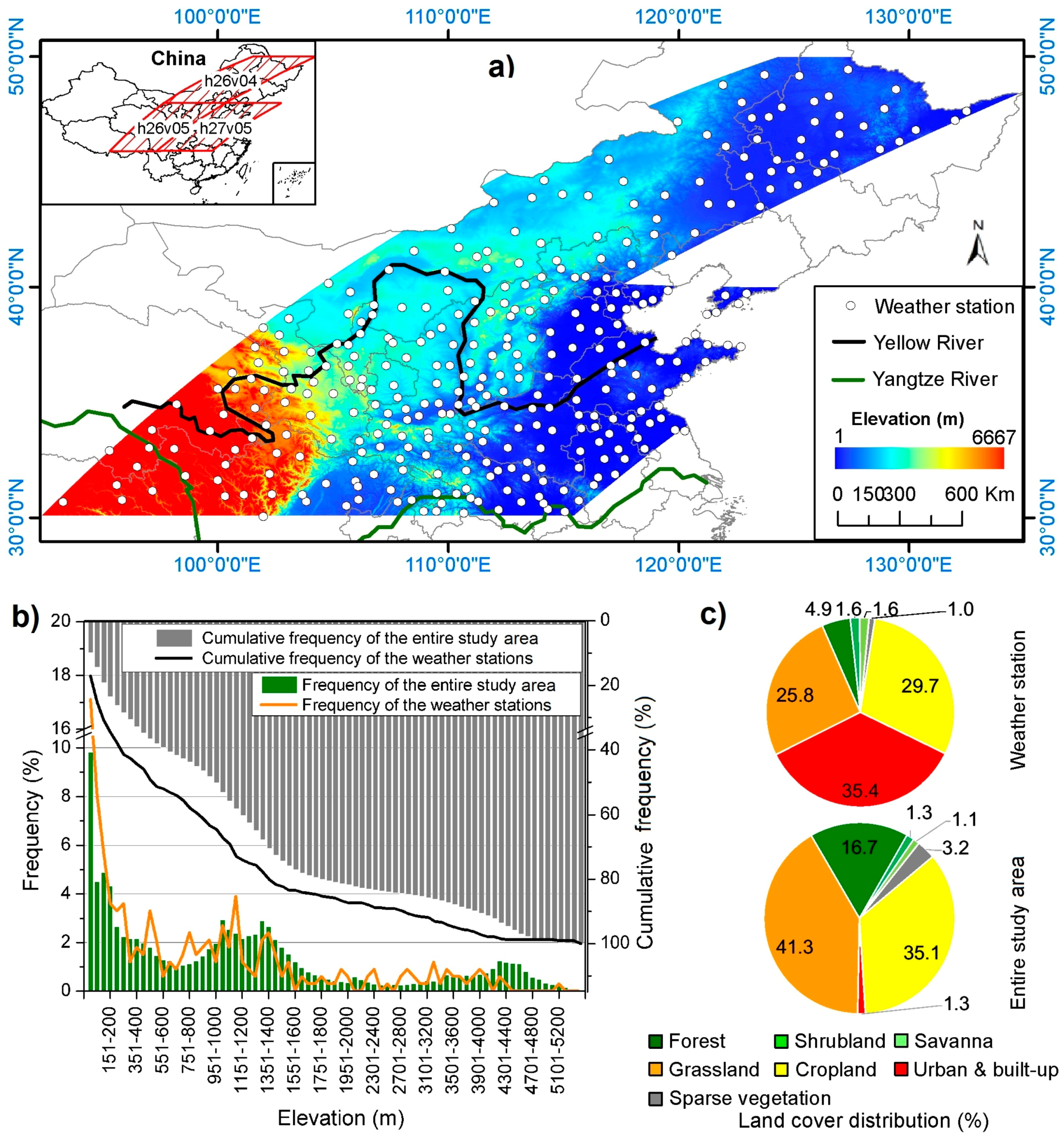
2.1. Study Area and Meteorological Data
2.2. Spatio-Temporal Predictors
2.2.1. LST
2.2.2. NDVI and ISA
2.2.3. BSA and NDWI
2.2.4. NSL
2.2.5. ELV
2.2.6. DDL
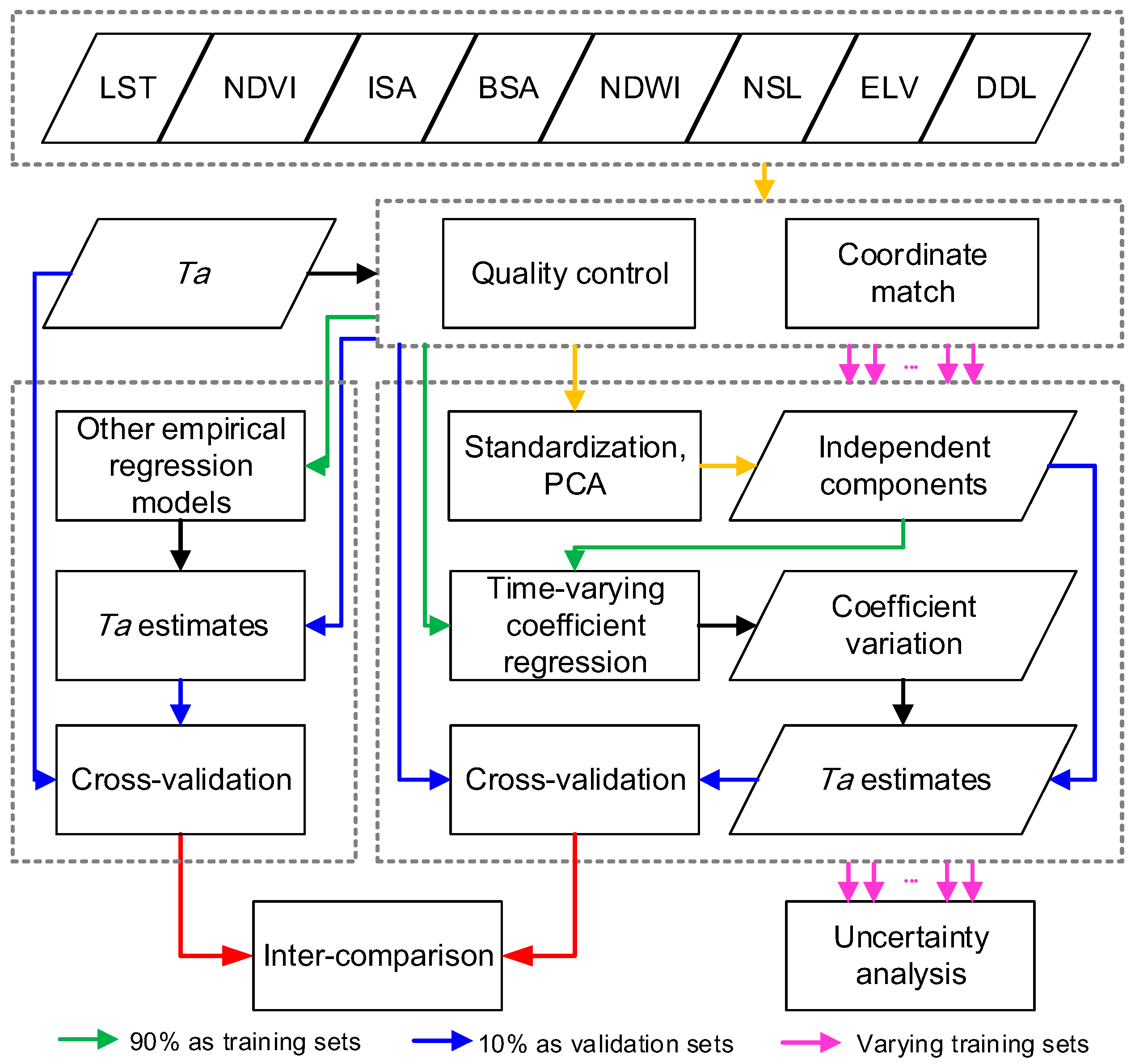
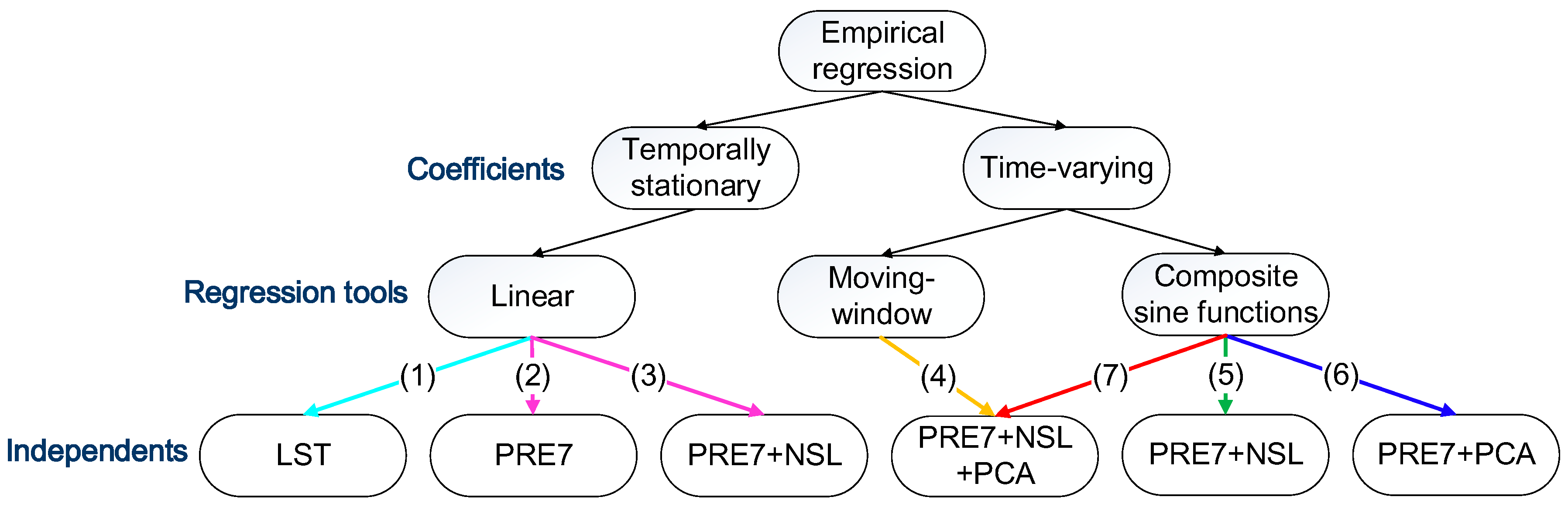
3. Methods
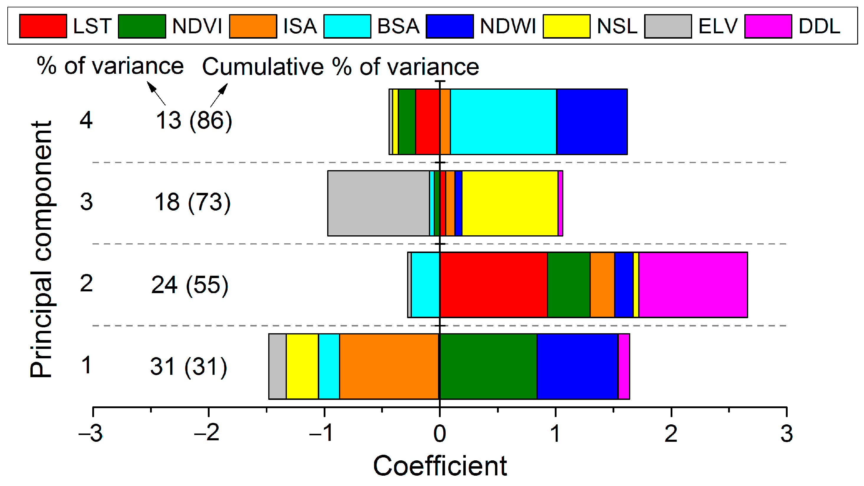
3.1. Independent Component Extraction
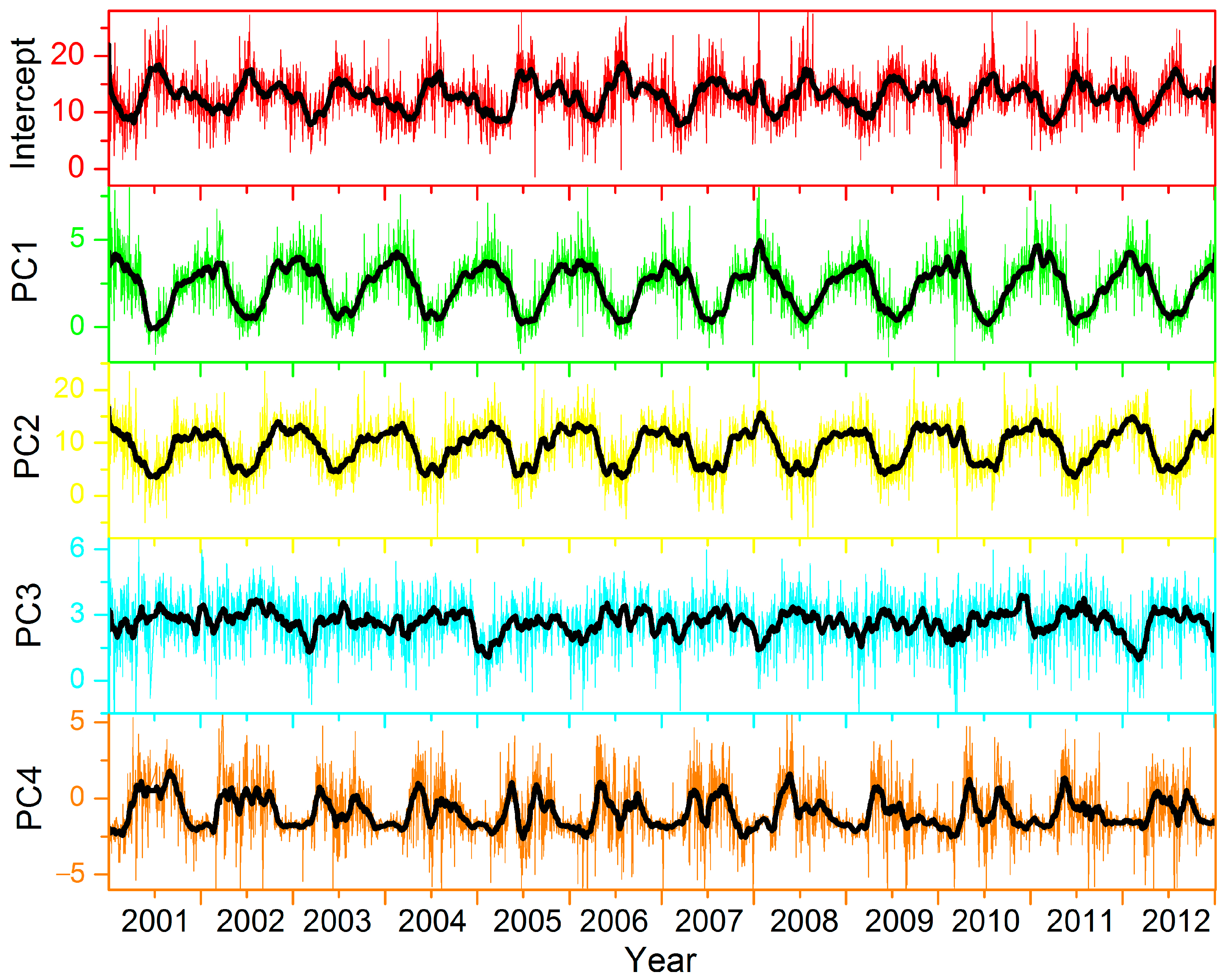
3.2. Time-Varying Coefficient Regression
3.3. Spatio-Temporal Ta Estimation
3.4. Model Evaluation
4. Results
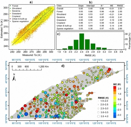
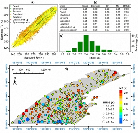
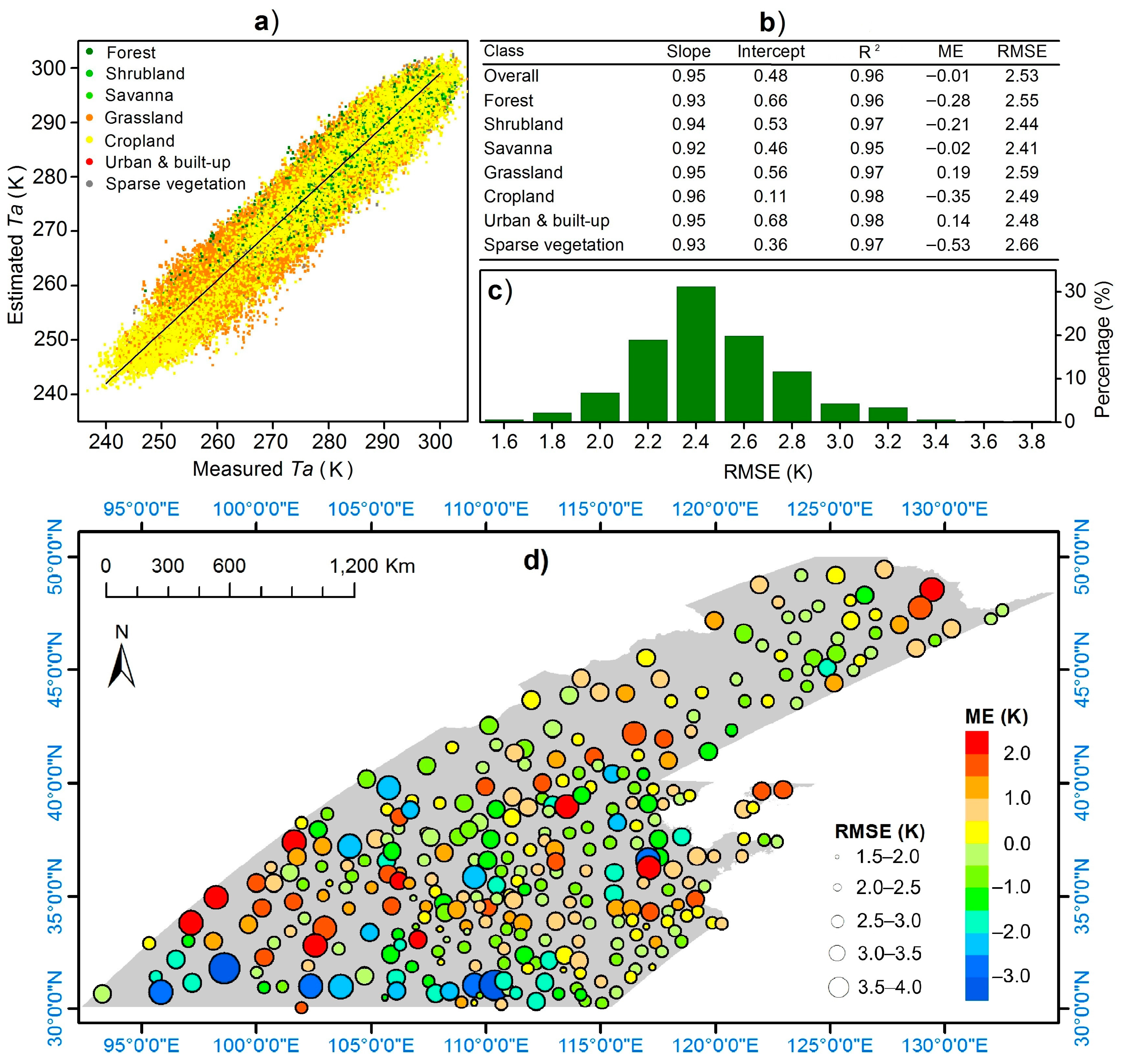
4.1. Spatial Patterns of Errors
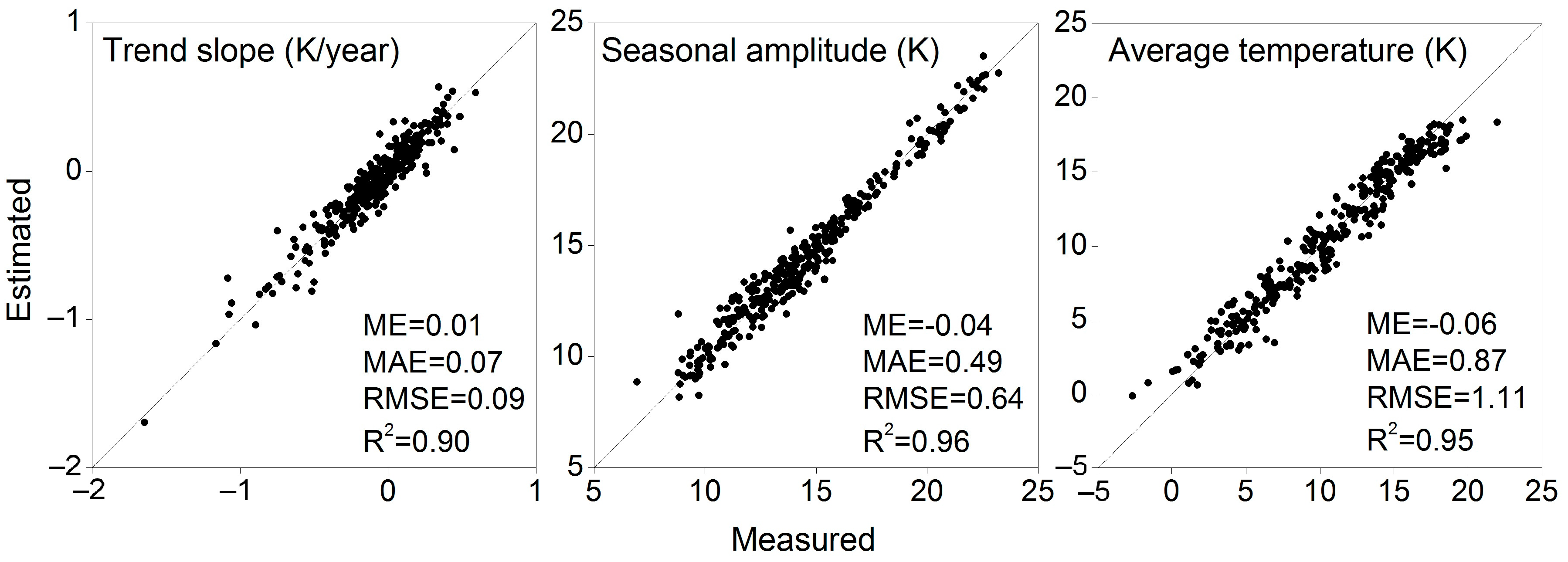
4.2. Temporal Patterns of Errors
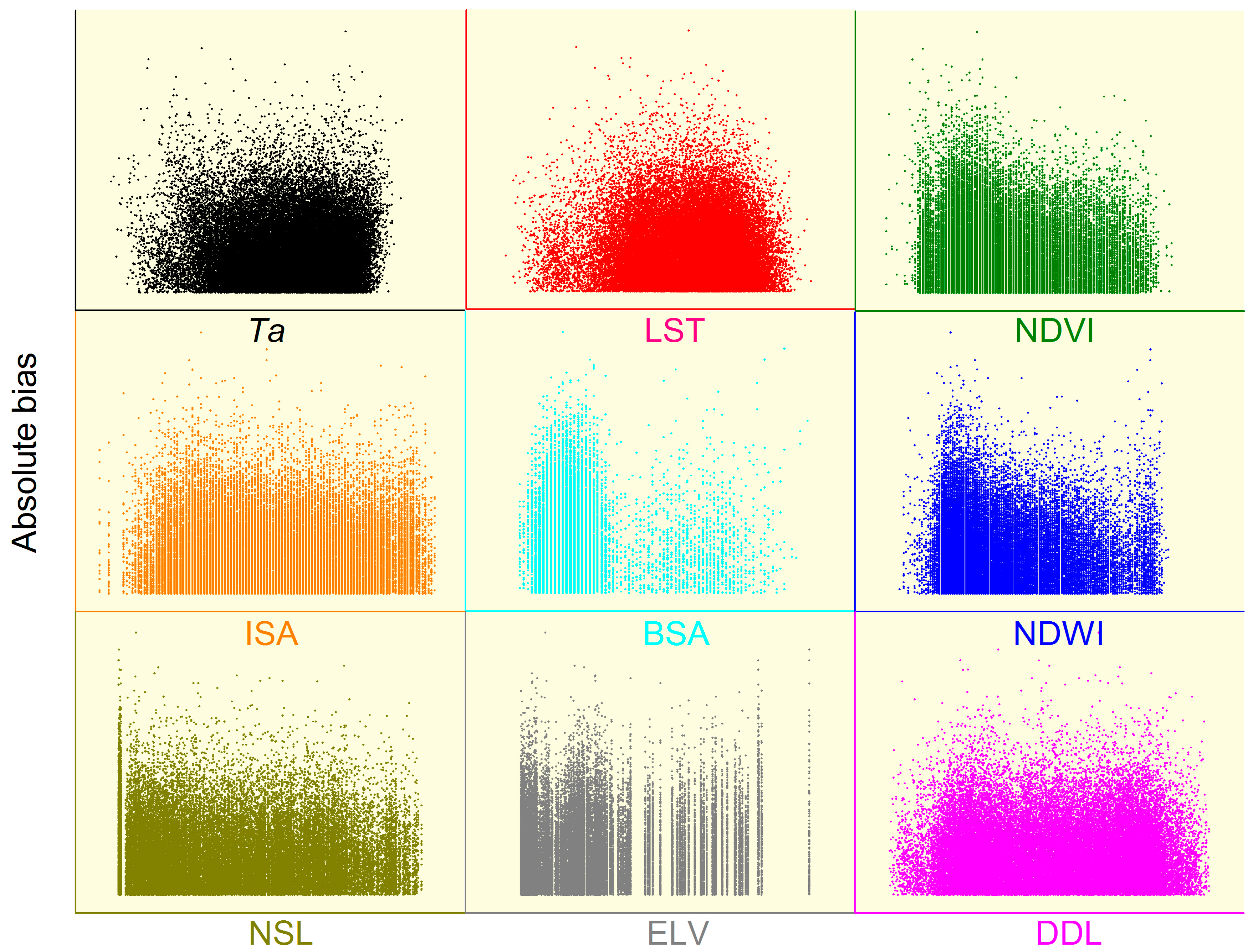
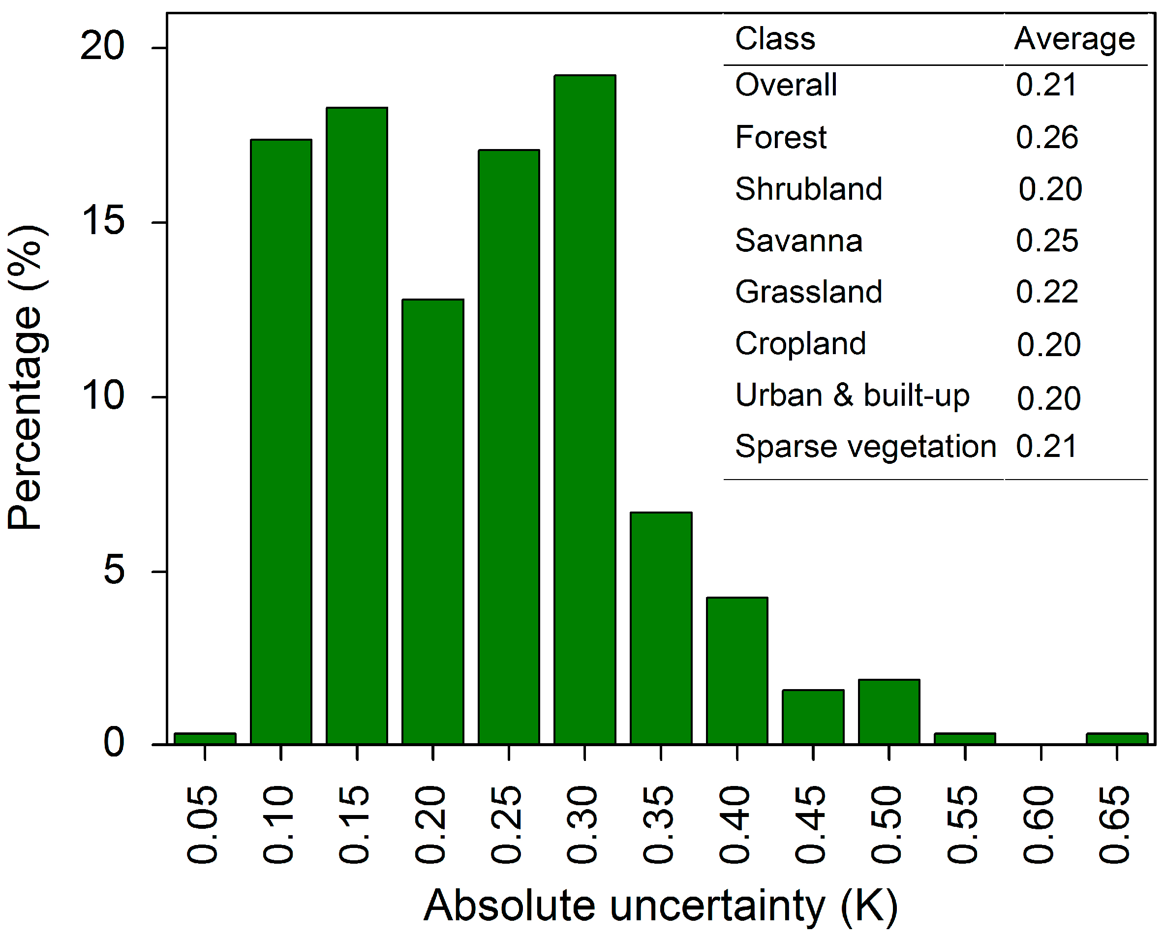
4.3. Uncertainty Analysis
4.4. Model Inter-comparison
5. Discussion
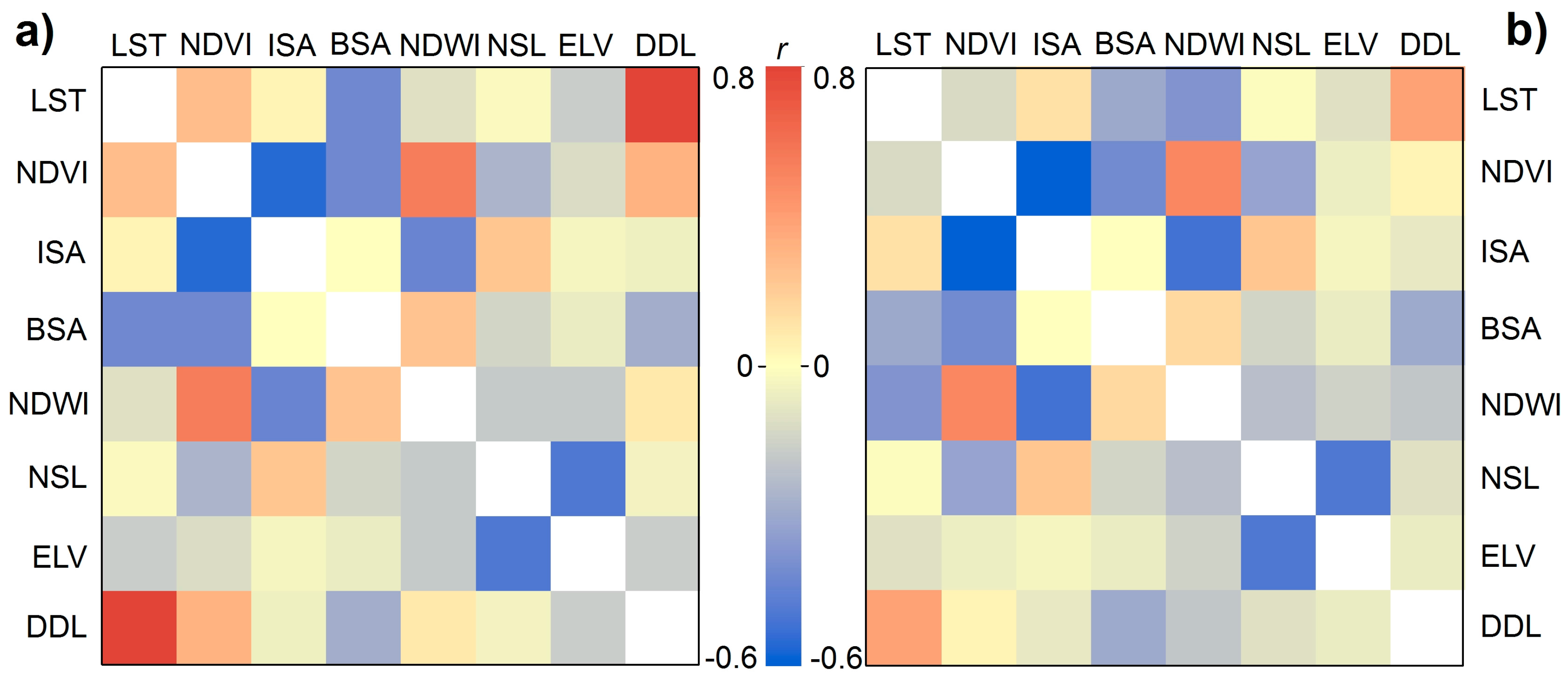
5.1. Nighttime Light, Predictor Independence, and Coefficient Dynamics
5.2. The Seven Predictors and Complementary Predictors
5.3. Spatio-Temporal Resolutions and Extensions
5.4. Ta Estimation under Cloudy Skies
6. Conclusions
Acknowledgments
Author Contributions
Conflicts of Interest
References
- Ho, H.C.; Knudby, A.; Sirovyak, P.; Xu, Y.; Hodul, M.; Henderson, S.B. Mapping maximum urban air temperature on hot summer days. Remote Sens. Environ. 2014, 154, 38–45. [Google Scholar] [CrossRef]
- Watson, R.T.; Albritton, D.L. Climate Change 2001: Synthesis Report: Third Assessment Report of the Intergovernmental Panel on Climate Change; Cambridge University Press: New York, NY, USA, 2001. [Google Scholar]
- Wang, L.; Koike, T.; Yang, K.; Yeh, P.J.F. Assessment of a distributed biosphere hydrological model against streamflow and MODIS land surface temperature in the upper tone river basin. J. Hydrol. 2009, 377, 21–34. [Google Scholar] [CrossRef]
- Garske, T.; Ferguson, N.M.; Ghani, A.C. Estimating air temperature and its influence on malaria transmission across Africa. PLoS ONE 2013, 8, e56487. [Google Scholar] [CrossRef] [PubMed]
- Nichol, J.E.; Wong, M.S. Spatial variability of air temperature and appropriate resolution for satellite-derived air temperature estimation. Int. J. Remote Sens. 2008, 29, 7213–7223. [Google Scholar] [CrossRef]
- Vancutsem, C.; Ceccato, P.; Dinku, T.; Connor, S.J. Evaluation of MODIS land surface temperature data to estimate air temperature in different ecosystems over Africa. Remote Sens. Environ. 2010, 114, 449–465. [Google Scholar] [CrossRef]
- Menzel, W.P.; Purdom, J.F.W. Introducing GOES-I: The first of a new generation of geostationary operational environmental satellites. Bull. Am. Meteorol. Soc. 1994, 75, 757–781. [Google Scholar] [CrossRef]
- Aumann, H.H.; Chahine, M.T.; Gautier, C.; Goldberg, M.D.; Kalnay, E.; McMillin, L.M.; Revercomb, H.; Rosenkranz, P.W.; Smith, W.L.; Staelin, D.H.; et al. AIRS/AMSU/HSB on the aqua mission: Design, science objectives, data products, and processing systems. IEEE Trans. Geosci. Remote Sens. 2003, 41, 253–264. [Google Scholar] [CrossRef]
- Borbas, E.E.; Seemann, S.W.; Aniko, K.; Moy, L.; Li, J.; Liam, G.; Menzel, W.P. MODIS Atmospheric Profile Retrieval Algorithm Theoretical Basis Document (collection 6); University of Wisconsin-Madison: Madison, WI, USA, 2011. [Google Scholar]
- Gao, W.; Zhao, F.; Xu, Y.; Feng, X. Validation of the surface air temperature products retrieved from the atmospheric infrared sounder over China. IEEE Trans. Geosci. Remote Sens. 2008, 46, 1783–1789. [Google Scholar]
- Sun, Y.J.; Wang, J.F.; Zhang, R.H.; Gillies, R.R.; Xue, Y.; Bo, Y.C. Air temperature retrieval from remote sensing data based on thermodynamics. Theor. Appl. Climatol. 2005, 80, 37–48. [Google Scholar] [CrossRef]
- Xu, Y.; Qin, Z.H.; Wan, H. Advances in the study of near surface air temperature retrieval from thermal infrared remote sensing. Remote Sens. Land. Resour. 2011, 9–14. [Google Scholar]
- Cristóbal, J.; Ninyerola, M.; Pons, X. Modeling air temperature through a combination of remote sensing and GIS data. J. Geophys. Res. Atmos. 2008, 113, D13106. [Google Scholar] [CrossRef]
- Florio, E.N.; Lele, S.R.; Chi Chang, Y.; Sterner, R.; Glass, G.E. Integrating AVHRR satellite data and NOAA ground observations to predict surface air temperature: A statistical approach. Int. J. Remote Sens. 2004, 25, 2979–2994. [Google Scholar] [CrossRef]
- Park, S. Integration of satellite-measured LST data into cokriging for temperature estimation on tropical and temperate islands. Int. J. Climatol. 2011, 31, 1653–1664. [Google Scholar] [CrossRef]
- Kilibarda, M.; Hengl, T.; Heuvelink, G.B.M.; Gräler, B.; Pebesma, E.; Perčec Tadić, M.; Bajat, B. Spatio-temporal interpolation of daily temperatures for global land areas at 1 km resolution. J. Geophys. Res. Atmos. 2014, 119, 2294–2313. [Google Scholar] [CrossRef]
- Chen, F.; Liu, Y.; Liu, Q.; Qin, F. A statistical method based on remote sensing for the estimation of air temperature in China. Int. J. Climatol. 2015, 35, 2131–2143. [Google Scholar] [CrossRef]
- Lennon, J.J.; Turner, J.R.G. Predicting the spatial distribution of climate: Temperature in great Britain. J. Anim. Ecol. 1995, 64, 370–392. [Google Scholar] [CrossRef]
- Stahl, K.; Moore, R.D.; Floyer, J.A.; Asplin, M.G.; McKendry, I.G. Comparison of approaches for spatial interpolation of daily air temperature in a large region with complex topography and highly variable station density. Agric. For. Meteorol. 2006, 139, 224–236. [Google Scholar] [CrossRef]
- Sun, H.; Chen, Y.; Gong, A.; Zhao, X.; Zhan, W.; Wang, M. Estimating mean air temperature using MODIS day and night land surface temperatures. Theor. Appl. Climatol. 2014, 118, 81–92. [Google Scholar] [CrossRef]
- Sandholt, I.; Rasmussen, K.; Andersen, J. A simple interpretation of the surface temperature/vegetation index space for assessment of surface moisture status. Remote Sens. Environ. 2002, 79, 213–224. [Google Scholar] [CrossRef]
- Stisen, S.; Sandholt, I.; Nørgaard, A.; Fensholt, R.; Eklundh, L. Estimation of diurnal air temperature using MSG SEVIRI data in West Africa. Remote Sens. Environ. 2007, 110, 262–274. [Google Scholar] [CrossRef]
- Xu, Y.; Qin, Z.; Shen, Y. Study on the estimation of near-surface air temperature from MODIS data by statistical methods. Int. J. Remote Sens. 2012, 33, 7629–7643. [Google Scholar] [CrossRef]
- Kloog, I.; Chudnovsky, A.; Koutrakis, P.; Schwartz, J. Temporal and spatial assessments of minimum air temperature using satellite surface temperature measurements in Massachusetts, USA. Sci. Total Environ. 2012, 432, 85–92. [Google Scholar] [CrossRef] [PubMed]
- Blennow, K. Modelling minimum air temperature in partially and clear felled forests. Agric. For. Meteorol. 1998, 91, 223–235. [Google Scholar] [CrossRef]
- Emamifar, S.; Rahimikhoob, A.; Noroozi, A.A. Daily mean air temperature estimation from MODIS land surface temperature products based on M5 model tree. Int. J. Climatol. 2013, 33, 3174–3181. [Google Scholar] [CrossRef]
- Shen, S.; Leptoukh, G.G. Estimation of surface air temperature over central and eastern Eurasia from MODIS land surface temperature. Environ. Res. Lett. 2011, 6, 045206. [Google Scholar] [CrossRef]
- Jang, J.D.; Viau, A.A.; Anctil, F. Neural network estimation of air temperatures from AVHRR data. Int. J. Remote Sens. 2004, 25, 4541–4554. [Google Scholar] [CrossRef]
- Benali, A.; Carvalho, A.C.; Nunes, J.P.; Carvalhais, N.; Santos, A. Estimating air surface temperature in Portugal using MODIS LST data. Remote Sens. Environ. 2012, 124, 108–121. [Google Scholar] [CrossRef]
- Fu, G.; Shen, Z.; Zhang, X.; Shi, P.; Zhang, Y.; Wu, J. Estimating air temperature of an alpine meadow on the northern Tibetan Plateau using MODIS land surface temperature. Acta Ecol. Sinica 2011, 31, 8–13. [Google Scholar] [CrossRef]
- Vogt, J.V.; Viau, A.A.; Paquet, F. Mapping regional air temperature fields using satellite-derived surface skin temperatures. Int. J. Climatol. 1997, 17, 1559–1579. [Google Scholar] [CrossRef]
- Muller, C.L.; Chapman, L.; Grimmond, C.S.B.; Young, D.T.; Cai, X. Sensors and the city: A review of urban meteorological networks. Int. J. Climatol. 2013, 33, 1585–1600. [Google Scholar] [CrossRef]
- Muller, C.L.; Chapman, L.; Grimmond, C.S.B.; Young, D.T.; Cai, X.-M. Toward a standardized metadata protocol for urban meteorological networks. Bull. Am. Meteorol. Soc. 2013, 94, 1161–1185. [Google Scholar] [CrossRef]
- Shao, Q.; Sun, C.; Liu, J.; He, J.; Kuang, W.; Tao, F. Impact of urban expansion on meteorological observation data and overestimation to regional air temperature in China. J. Geogr. Sci. 2011, 21, 994–1006. [Google Scholar] [CrossRef]
- Good, E. Daily minimum and maximum surface air temperatures from geostationary satellite data. J. Geophys. Res. Atmos. 2015, 120, 2306–2324. [Google Scholar] [CrossRef]
- Nichol, J.E.; To, P.H. Temporal characteristics of thermal satellite images for urban heat stress and heat island mapping. ISPRS J. Photogramm. Remote Sens. 2012, 74, 153–162. [Google Scholar] [CrossRef]
- Sailor, D.J.; Lu, L. A top down methodology for developing diurnal and seasonal anthropogenic heating profiles for urban areas. Atmos. Environ. 2004, 38, 2737–2748. [Google Scholar] [CrossRef]
- Fan, H.; Sailor, D.J. Modeling the impacts of anthropogenic heating on the urban climate of Philadelphia: A comparison of implementations in two PBL schemes. Atmos. Environ. 2005, 39, 73–84. [Google Scholar] [CrossRef]
- Salamanca, F.; Georgescu, M.; Mahalov, A.; Moustaoui, M.; Wang, M. Anthropogenic heating of the urban environment due to air conditioning. J. Geophys. Res. Atmos. 2014, 119, 5949–5965. [Google Scholar] [CrossRef]
- Oke, T.R. The urban energy balance. Progr. Phys. Geogr. 1988, 12, 471–508. [Google Scholar] [CrossRef]
- Taha, H.; Akbari, H.; Sailor, D.; Ritschard, R. Causes and Effects of Heat Islands: Sensitivity to Surface Parameters and Anthropogenic Heating; Lawrence Berkeley Lab: Berkeley, CA, USA, 1992.
- Sailor, D.J.; Georgescu, M.; Milne, J.M.; Hart, M.A. Development of a national anthropogenic heating database with an extrapolation for international cities. Atmos. Environ. 2015, 118, 7–18. [Google Scholar] [CrossRef]
- Kato, S.; Yamaguchi, Y. Analysis of urban heat-island effect using ASTER and ETM+ data: Separation of anthropogenic heat discharge and natural heat radiation from sensible heat flux. Remote Sens. Environ. 2005, 99, 44–54. [Google Scholar] [CrossRef]
- Chen, B.; Shi, G.; Wang, B.; Zhao, J.; Tan, S. Estimation of the anthropogenic heat release distribution in China from 1992 to 2009. Acta Meteorol. Sinica 2012, 26, 507–515. [Google Scholar] [CrossRef]
- Dormann, C.F.; Elith, J.; Bacher, S.; Buchmann, C.; Carl, G.; Carré, G.; Marquéz, J.R.G.; Gruber, B.; Lafourcade, B.; Leitão, P.J.; et al. Collinearity: A review of methods to deal with it and a simulation study evaluating their performance. Ecography 2013, 36, 27–46. [Google Scholar] [CrossRef]
- Lee, J.S. The Geology of China; Thomas Murky & Co.: London, UK, 1939; p. 31. [Google Scholar]
- Zhou, D.C.; Zhao, S.Q.; Liu, S.G.; Zhang, L.X.; Zhu, C. Surface urban heat island in China's 32 major cities: Spatial patterns and drivers. Remote Sens. Environ. 2014, 152, 51–61. [Google Scholar] [CrossRef]
- Angstrom, A. Solar and terrestrial radiation. Report to the international commission for solar research on actinometric investigations of solar and atmospheric radiation. Q. J. R. Meteorol. Soc. 1924, 50, 121–126. [Google Scholar] [CrossRef]
- Wan, Z.M.; Dozier, J. A generalized split-window algorithm for retrieving land-surface temperature from space. IEEE Trans. Geosci. Remote Sens. 1996, 34, 892–905. [Google Scholar]
- Wan, Z.M. New refinements and validation of the collection-6 MODIS land-surface temperature/emissivity product. Remote Sens. Environ. 2014, 140, 36–45. [Google Scholar] [CrossRef]
- Hulley, G.C.; Hughes, C.G.; Hook, S.J. Quantifying uncertainties in land surface temperature and emissivity retrievals from aster and MODIS thermal infrared data. J. Geophys. Res. 2012, 117, D23113. [Google Scholar] [CrossRef]
- Wan, Z.M. New refinements and validation of the MODIS land-surface temperature/emissivity products. Remote Sens. Environ. 2008, 112, 59–74. [Google Scholar] [CrossRef]
- Neteler, M. Estimating daily land surface temperatures in mountainous environments by reconstructed MODIS LST data. Remote Sens. 2010, 2, 333–351. [Google Scholar] [CrossRef]
- Wang, K.; Liang, S. Evaluation of aster and MODIS land surface temperature and emissivity products using long-term surface longwave radiation observations at SURFRAD sites. Remote Sens. Environ. 2009, 113, 1556–1565. [Google Scholar] [CrossRef]
- Wang, W.; Liang, S.; Meyers, T. Validating MODIS land surface temperature products using long-term nighttime ground measurements. Remote Sens. Environ. 2008, 112, 623–635. [Google Scholar] [CrossRef]
- Lagouarde, J.P.; Hénon, A.; Irvine, M.; Voogt, J.; Pigeon, G.; Moreau, P.; Masson, V.; Mestayer, P. Experimental characterization and modelling of the nighttime directional anisotropy of thermal infrared measurements over an urban area: Case study of Toulouse (France). Remote Sens. Environ. 2012, 117, 19–33. [Google Scholar] [CrossRef]
- Quan, J.L.; Chen, Y.H.; Zhan, W.F.; Wang, J.F.; Voogt, J.; Wang, M.J. Multi-temporal trajectory of the urban heat island centroid in Beijing, China based on a Gaussian volume model. Remote Sens. Environ. 2014, 149, 33–46. [Google Scholar] [CrossRef]
- Yang, F.; Matsushita, B.; Fukushima, T.; Yang, W. Temporal mixture analysis for estimating impervious surface area from multi-temporal MODIS NDVI data in Japan. ISPRS J. Photogramm. Remote Sens. 2012, 72, 90–98. [Google Scholar] [CrossRef] [Green Version]
- Abraha, M.G.; Savage, M.J. Comparison of estimates of daily solar radiation from air temperature range for application in crop simulations. Agric. For. Meteorol. 2008, 148, 401–416. [Google Scholar] [CrossRef]
- Gao, B.C. NDWI A normalized difference water index for remote sensing of vegetation liquid water from space. Remote Sens. Environ. 1996, 58, 257–266. [Google Scholar] [CrossRef]
- Liu, Z.; He, C.; Zhang, Q.; Huang, Q.; Yang, Y. Extracting the dynamics of urban expansion in China using DMSP-OLS nighttime light data from 1992 to 2008. Landsc. Urban Plan. 2012, 106, 62–72. [Google Scholar] [CrossRef]
- Elvidge, C.D.; Ziskin, D.; Baugh, K.E.; Tuttle, B.T.; Ghosh, T.; Pack, D.W.; Erwin, E.H.; Zhizhin, M. A fifteen year record of global natural gas flaring derived from satellite data. Energies 2009, 2, 595–622. [Google Scholar] [CrossRef]
- Ma, T.; Zhou, Y.; Zhou, C.; Haynie, S.; Pei, T.; Xu, T. Night-time light derived estimation of spatio-temporal characteristics of urbanization dynamics using DMSP/OLS satellite data. Remote Sens. Environ. 2015, 158, 453–464. [Google Scholar] [CrossRef]
- Göttsche, F.M.; Olesen, F.S. Modelling of diurnal cycles of brightness temperature extracted from Meteosat data. Remote Sens. Environ. 2001, 76, 337–348. [Google Scholar] [CrossRef]
- Rajagopalan, B.; Lall, U. A k-nearest-neighbor simulator for daily precipitation and other weather variables. Water Resour. Res. 1999, 10, 3089–3101. [Google Scholar] [CrossRef]
- Singh, A.; Harrison, A. Standardized principal components. Int. J. Remote Sens. 1985, 6, 883–896. [Google Scholar] [CrossRef]
- Jain, A.; Nandakumar, K.; Ross, A. Score normalization in multimodal biometric systems. Pattern Recognit. 2005, 38, 2270–2285. [Google Scholar] [CrossRef]
- Zakšek, K.; Oštir, K. Downscaling land surface temperature for urban heat island diurnal cycle analysis. Remote Sens. Environ. 2012, 117, 114–124. [Google Scholar] [CrossRef]
- Quan, J.L.; Zhan, W.F.; Chen, Y.H.; Wang, M.; Wang, J.F. Time series decomposition of remotely sensed land surface temperature and investigation of trends and seasonal variations in surface urban heat islands. J. Geophys. Res. Atmos. 2016, 121, 2638–2657. [Google Scholar] [CrossRef]
- Amaral, S.; Monteiro, A.M.V.; Camara, G.; Quintanilha, J.A. DMSP/OLS nighttime light imagery for urban population estimates in the Brazilian Amazon. Int. J. Remote Sens. 2006, 27, 855–870. [Google Scholar] [CrossRef]
- Ghosh, T.; Anderson, S.; Powell, L.R.; Sutton, C.P.; Elvidge, D.C. Estimation of Mexico's informal economy and remittances using nighttime imagery. Remote Sens. 2009, 1, 418–444. [Google Scholar] [CrossRef]
- Letu, H.; Hara, M.; Yagi, H.; Naoki, K.; Tana, G.; Nishio, F.; Shuhei, O. Estimating energy consumption from night-time DMPS/OLS imagery after correcting for saturation effects. Int. J. Remote Sens. 2010, 31, 4443–4458. [Google Scholar] [CrossRef]
- Bechtel, B.; Zakšek, K.; Hoshyaripour, G. Downscaling land surface temperature in an urban area: A case study for Hamburg, Germany. Remote Sens. 2012, 4, 3184–3200. [Google Scholar] [CrossRef]
- Gu, Y.; Hunt, E.; Wardlow, B.; Basara, J.B.; Brown, J.F.; Verdin, J.P. Evaluation of MODIS NDVI and NDWI for vegetation drought monitoring using Oklahoma Mesonet soil moisture data. Geophys. Res. Lett. 2008, 35, L22401. [Google Scholar] [CrossRef]
- Rizwan, A.M.; Dennis, L.Y.C.; Liu, C. A review on the generation, determination and mitigation of urban heat island. J. Environ. Sci. 2008, 20, 120–128. [Google Scholar] [CrossRef]
- Janjai, S.; Pankaew, P.; Laksanaboonsong, J.; Kitichantaropas, P. Estimation of solar radiation over cambodia from long-term satellite data. Renew. Energy 2011, 36, 1214–1220. [Google Scholar] [CrossRef]
- Reddy, K.S.; Ranjan, M. Solar resource estimation using artificial neural networks and comparison with other correlation models. Energy Conv. Manag. 2003, 44, 2519–2530. [Google Scholar] [CrossRef]
- Soltani, A.; Meinke, H.; de Voil, P. Assessing linear interpolation to generate daily radiation and temperature data for use in crop simulations. Eur. J. Agron. 2004, 21, 133–148. [Google Scholar] [CrossRef]
- Bristow, K.L.; Campbell, G.S. On the relationship between incoming solar radiation and daily maximum and minimum temperature. Agric. For. Meteorol. 1984, 31, 159–166. [Google Scholar] [CrossRef]
- Mahmood, R.; Hubbard, K.G. Effect of time of temperature observation and estimation of daily solar radiation for the Northern Great Plains, USA. Agron. J. 2002, 94, 723–733. [Google Scholar] [CrossRef]
- Hansen, J.W. Stochastic daily solar irradiance for biological modeling applications. Agric. For. Meteorol. 1999, 94, 53–63. [Google Scholar] [CrossRef]
- Zakšek, K.; Podobnikar, T.; Oštir, K. Solar radiation modelling. Comput. Geosci. 2005, 31, 233–240. [Google Scholar] [CrossRef]
- Avissar, R.; Pielke, R.A. A parameterization of heterogeneous land surfaces for atmospheric numerical models and its impact on regional meteorology. Mon. Weather Rev. 1989, 117, 2113–2136. [Google Scholar] [CrossRef]
- Huang, H.-Y.; Margulis, S.A. On the impact of surface heterogeneity on a realistic convective boundary layer. Water Resour. Res. 2009, 45, W04425. [Google Scholar] [CrossRef]
- Garrigues, S.; Allard, D.; Baret, F.; Weiss, M. Quantifying spatial heterogeneity at the landscape scale using variogram models. Remote Sens. Environ. 2006, 103, 81–96. [Google Scholar] [CrossRef]
- Hintz, M.; Lennartz-Sassinek, S.; Liu, S.; Shao, Y. Quantification of land surface heterogeneity via entropy spectrum method. J. Geophys. Res. Atmos. 2014, 119, 8764–8777. [Google Scholar] [CrossRef]
- Chen, Y.H.; Shi, P.J.; Li, X.B. Research on spatial thermal environment in Shanghai city based on remote sensing and GIS. Acta Geod. Cartogr. Sinica 2002, 31, 139–144. [Google Scholar]
- Unger, J. Intra-urban relationship between surface geometry and urban heat island: Review and new approach. Clim. Res. 2004, 27, 253–264. [Google Scholar] [CrossRef]
- Hu, D.; Yang, L.M.; Zhou, J.; Deng, L. Estimation of urban energy heat flux and anthropogenic heat discharge using ASTER image and meteorological data: Case study in Beijing metropolitan area. J. Appl. Remote Sens. 2012, 6, 063559. [Google Scholar] [CrossRef]
- Holden, Z.A.; Abatzoglou, J.T.; Luce, C.H.; Baggett, S.L. Empirical downscaling of daily minimum air temperature at very fine resolutions in complex terrain. Agric. For. Meteorol. 2011, 151, 1066–1073. [Google Scholar] [CrossRef]
- Bechtel, B.; Wiesner, S.; Zakšek, K. Estimation of dense time series of urban air temperatures from multitemporal geostationary satellite data. IEEE J. Sel. Top. Appl. Earth Obs. Remote Sens. 2014, 7, 4129–4137. [Google Scholar] [CrossRef]
- Kloog, I.; Nordio, F.; Coull, B.A.; Schwartz, J. Predicting spatiotemporal mean air temperature using MODIS satellite surface temperature measurements across the northeastern USA. Remote Sens. Environ. 2014, 150, 132–139. [Google Scholar] [CrossRef]
- Jin, M.; Dickinson, R.E. Land surface skin temperature climatology: Benefitting from the strengths of satellite observations. Environ. Res. Lett. 2010, 5, 044004. [Google Scholar] [CrossRef]
- Pepin, N.C.; Norris, J.R. An examination of the differences between surface and free-air temperature trend at high-elevation sites: Relationships with cloud cover, snow cover, and wind. J. Geophys. Res. Atmos. 2005, 110, D24112. [Google Scholar] [CrossRef]
- Jang, K.; Kang, S.; Kimball, S.J.; Hong, Y.S. Retrievals of all-weather daily air temperature using MODIS and AMSR-E data. Remote Sens. 2014, 6, 8387–8404. [Google Scholar] [CrossRef]
- Jones, L.A.; Ferguson, C.R.; Kimball, J.S.; Zhang, K.; Chan, S.T.K.; McDonald, K.C.; Njoku, E.G.; Wood, E.F. Satellite microwave remote sensing of daily land surface air temperature minima and maxima from amsr-e. IEEE J. Sel. Top. Appl. Earth Obs. Remote Sens. 2010, 3, 111–123. [Google Scholar] [CrossRef]
- Köhn, J.; Royer, A. Microwave brightness temperature as an indicator of near-surface air temperature over snow in Canadian northern regions. Int. J. Remote Sens. 2012, 33, 1126–1138. [Google Scholar] [CrossRef]
- Zhan, W.; Zhou, J.; Ju, W.; Li, M.; Sandholt, I.; Voogt, J.; Yu, C. Remotely sensed soil temperatures beneath snow-free skin-surface using thermal observations from tandem polar-orbiting satellites: An analytical three-time-scale model. Remote Sens. Environ. 2014, 143, 1–14. [Google Scholar] [CrossRef]


| Predictor | Source | Spatial Resolution | Temporal Resolution |
|---|---|---|---|
| Land surface temperature (LST) | MOD11A1 (~22:30) | 1000 m | 1 day |
| Normalized difference vegetation index (NDVI) | MOD13Q1 (~10:30) | 250 m | 16 days |
| Impervious surface area (ISA) | Temporal mixture analysis of NDVI time series | 250 m | 1 year |
| Black-sky albedo (BSA) | MCD43A3 | 500 m | 16 days |
| Normalized difference water index (NDWI) | Calculated from BSA | 500 m | 16 days |
| Nighttime stable light (NSL) | DMSP/OLS | 30″ | 1 year |
| Elevation (ELV) | GTOPO30 | 30″ | - |
| Duration of daylight (DDL) | Calculated from latitude and day of year | 1000 m | 1 day |
| Year | RMSE (K) | R2 | Month | RMSE (K) | R2 | Season | RMSE (K) | R2 |
|---|---|---|---|---|---|---|---|---|
| 2001 | 2.55 | 0.97 | December | 2.46 | 0.93 | Winter | 2.53 | 0.98 |
| 2002 | 2.56 | 0.98 | January | 2.61 | 0.93 | |||
| 2003 | 2.45 | 0.98 | February | 2.62 | 0.92 | |||
| 2004 | 2.53 | 0.97 | March | 2.63 | 0.90 | Spring | 2.62 | 0.92 |
| 2005 | 2.51 | 0.98 | April | 2.63 | 0.88 | |||
| 2006 | 2.56 | 0.97 | May | 2.61 | 0.85 | |||
| 2007 | 2.44 | 0.98 | June | 2.53 | 0.85 | Summer | 2.50 | 0.90 |
| 2008 | 2.45 | 0.98 | July | 2.44 | 0.88 | |||
| 2009 | 2.56 | 0.98 | August | 2.40 | 0.87 | |||
| 2010 | 2.60 | 0.98 | September | 2.46 | 0.87 | Autumn | 2.47 | 0.93 |
| 2011 | 2.64 | 0.98 | October | 2.50 | 0.90 | |||
| 2012 | 2.52 | 0.98 | November | 2.42 | 0.93 | |||
| Model | RMSE (K) | R2 |
|---|---|---|
| (1) Linear regression with LST | 5.13 | 0.89 |
| (2) Linear regression with the seven predictors (excluding NSL) | 3.35 | 0.94 |
| (3) Linear regression with the eight predictors | 3.33 | 0.96 |
| (4) Moving-window regression with PC1–PC4 of the eight predictors | 2.71 | 0.81 |
| (5) Composite sinusoidal coefficient regression with the eight predictors | - | - |
| (6) Composite sinusoidal coefficient regression with PC1–PC4 of the seven predictors (excluding NSL) | 3.11 | 0.96 |
| (7) Composite sinusoidal coefficient regression with PC1–PC4 of the eight predictors | 2.53 | 0.96 |
| Predictor Excluded | ΔRMSE (K) | ΔR2 | Predictor Excluded | ΔRMSE (K) | ΔR2 |
|---|---|---|---|---|---|
| LST | 1.59 | 0.06 | NDWI | 0.30 | 0.02 |
| NDVI | 0.04 | 0.00 | ELV | 0.30 | 0.02 |
| ISA | 0.14 | 0.00 | DDL | 0.20 | 0.02 |
| BSA | 0.22 | 0.02 |
© 2016 by the authors; licensee MDPI, Basel, Switzerland. This article is an open access article distributed under the terms and conditions of the Creative Commons Attribution (CC-BY) license (http://creativecommons.org/licenses/by/4.0/).
Share and Cite
Chen, Y.; Quan, J.; Zhan, W.; Guo, Z. Enhanced Statistical Estimation of Air Temperature Incorporating Nighttime Light Data. Remote Sens. 2016, 8, 656. https://doi.org/10.3390/rs8080656
Chen Y, Quan J, Zhan W, Guo Z. Enhanced Statistical Estimation of Air Temperature Incorporating Nighttime Light Data. Remote Sensing. 2016; 8(8):656. https://doi.org/10.3390/rs8080656
Chicago/Turabian StyleChen, Yunhao, Jinling Quan, Wenfeng Zhan, and Zheng Guo. 2016. "Enhanced Statistical Estimation of Air Temperature Incorporating Nighttime Light Data" Remote Sensing 8, no. 8: 656. https://doi.org/10.3390/rs8080656