Downscaling Snow Cover Fraction Data in Mountainous Regions Based on Simulated Inhomogeneous Snow Ablation

Abstract

High-resolution snow distributions are essential for studying cold regions. However, the temporal and spatial resolutions of current remote sensing snow maps remain limited. Remotely sensed snow cover fraction (SCF) data only provide quantitative descriptions of snow area proportions and do not provide information on subgrid-scale snow locations. We present a downscaling method based on simulated inhomogeneous snow ablation capacities that are driven by air temperature and solar radiation data. This method employs a single parameter to adjust potential snow ablation capacities. Using this method, SCF data with a resolution of 500 m are downscaled to a resolution of 30 m. Then, 18 remotely sensed TM, CHRIS and EO-1 snow maps are used to verify the downscaled results. The mean overall accuracy is 0.69, the average root-mean-square error (RMSE) of snow-covered slopes between the downscaled snow map and the real snow map is 3.9°, and the average RMSE of the sine of the snow covered aspects between the downscaled snow map and the real snow map is 0.34, which is equivalent to 19.9°. This method can be applied to high-resolution snow mapping in similar mountainous regions.

1. Introduction

Accurate snow spatial heterogeneity descriptions are essential to scientific studies in cold regions [1]. Snow distributions present high degrees of heterogeneity under complex terrain conditions [2,3]. Only high-spatial-resolution snow maps can be used to accurately characterize the patterns of snow distribution and melting in such regions. This paper aims to provide a method retrieving subgrid-scale snowpack locations by downscaling remotely sensed snow cover fraction data.

The limited available studies of the spatial heterogeneity of subgrid-scale snow cover have indicated that using different grid sizes while modeling distributed snowmelt can result in considerable variability in modeling accuracy [4]. For hydrological simulations conducted in cold regions, there are various flow routing paths for distributed snowpack at various points in a spatial grid [5]. Moreover, accurate descriptions of the snow’s spatial heterogeneity are essential to estimating solar radiation in snow-covered mountainous areas [6]. These works further underscore the importance of obtaining accurate, high-resolution snow distributions.

With the rapid development of remote sensing (RS) technologies, highly accurate snow cover area (SCA) measurements can now be retrieved at various spatial and temporal resolutions [7]. While some high-spatial-resolution satellite images for snow mapping exist (e.g., IKONOS [8] and Landsat/TM (Thematic Mapper) [9,10]), these images are generated over long time intervals (e.g., 16 days for the TM). In gathering more detailed information, scientists have examined methods for retrieving MODIS (MODerate-resolution Imaging Spectroradiometer) fractional snow cover (SCF) data at the pixel scale [11,12]. Successful retrieval algorithms include the normalized difference snow index method [13] and the linear spectral mixture analysis method [14]. These remotely sensed SCF data have been used in various land-surface [15] and hydrological models [2,16] to represent snow distribution heterogeneity. Recently, SCF products, particularly MODIS data, have become more popular than binary snow mapping data. Although SCF data are frequently affected by cloud cover, several effective cloud removal methods exist [17,18,19].

However, subgrid-scale snow locations remain unknown when SCF data products are used, which can introduce considerable errors when estimating patterns of solar radiation or snowmelt flow paths in mountainous regions. It is also of interest to map subgrid-scale snow locations in mountainous regions in accurate geoscientific studies. Few published works have attempted this task. For example, Walters et al. [20] downscaled MODIS fractional snow cover data using topographic snow distribution features, and Czyzowska-Wisniewski et al. [8] estimated snow cover distributions by fusing multi-sensor remotely sensed data with medium temporal/spatial resolutions over complex terrain. While these methods can retrieve subgrid-scale snow locations, they do not consider temporal and spatial features of snow ablation processes. Some studies focused on the relationship between the statistical probability distribution of snow water equivalent and the sub-grid terrain characteristics at the subgrid scale [21,22,23], and other studies estimated snow water equivalent according to known snow cover area at the subgrid scale, via a parameterized snow depletion curve [24,25]. For better ablation simulation, some studies evaluated the influence of resolution and topographic uncertainty on modelling melt at the subgrid scale [26]. However, these studies did not take into account subgrid-scale snowpack locations and the influence of temporal weather conditions on inhomogeneous snow ablation.

Beyond the studies above, this study develops a means of retrieving subgrid-scale snowpack locations via simulated inhomogeneous snow ablation. In this method, air temperature and solar radiation data, more than just DEM (Digital Elevation Model) data, are integrated together to downscale snow cover fraction data. Inhomogeneous snow ablation results in heterogeneous snow distribution at the subgrid scale. It is necessary to determine the inhomogeneity in order to determine snow patterns and locations at the subgrid scale. The inhomogeneity can be simulated by an empirical snowmelt model driven by air temperature and solar radiation at the subgrid scale. Simulated inhomogeneous snow ablations are considered a priori information to downscale snow cover fraction at the subgrid scale in this study. This method can better reflect the temporal and spatial inhomogeneous characteristic of snow ablation. The presented method is based on the following principles:

(1)

Snow is always present where it is not easily ablated, such as northern slopes and high-altitude regions. In a grid with complex terrain, snow ablation capacities differ from topographies.

(2)

Inhomogeneous snow ablation capacities can be empirically simulated based on dominant meteorological factors, such as solar radiation and air temperature. Solar radiation and air temperature can be accurately interpolated using a limited number of station observations [27].

(3)

Comparing modeled ablation heterogeneities at the subgrid scale enables one to allocate snow positions where snow is not easily ablated under a given grid-scale SCF.

2. Methodology

2.1. Problem Description

The problem to be solved is as follows. Given a known grid-scale SCF, a finer subgrid-scale DEM and a meteorological data time series, can we estimate subgrid-scale snow locations? The following values are given:

(1)

A grid measuring L by L and containing n times n cells.

(2)

A grid-scale SCF (≤100%) of the grid at time t.

(3)

A subgrid-scale DEM with a spatial resolution of L/n.

(4)

A subgrid-scale time series of solar radiation and air temperature in a typical snow season.

Specifically, then, which cells are snow-covered?

Solution: We use the potential snow ablation capacity P_s principle to quantitatively estimate the presence of snow. In this study, P_s is computed using an improved degree-day factor method that takes into account the radiation index (see Section 2.2). Three assumptions are made. (1) Snow is present for longer periods of time where snow ablation is relatively low, e.g., on north-facing slopes or at high altitudes; (2) precipitation is homogeneous within a grid; (3) the subgrid is the basic unit, and subgrid-scale ablation is homogeneous.

In this study, the grid scale is set to 500 m, thereby matching the typical spatial resolution of the fractional snow cover data (e.g., MODIS), and the subgrid scale is set to 30 m, as in high-resolution remotely sensed images (e.g., TM).

For convenience, the abbreviation DS subgrids denotes those subgrids classified as snow-covered in the downscaled snow map, and RS subgrids denotes snow-covered pixels (subgrids) in the high-resolution remotely sensed snow maps.

2.2. Calculation of Potential Snow Ablation Capacities

P_s is defined as the total subgrid-scale snow ablation from the first day of a snow season (i = 1) until the date on which the SCF data are downscaled (i = t), assuming that enough snow has ablated. For the ith subgrid,

$$P_s^i={\displaystyle \sum _{i=1}^t(k_d{T}_i+k_r{R}_i)}$$

(1)

where k_d (cm·°C⁻¹·day⁻¹) is the degree-day factor. A degree-day factor indicates the snowmelt depth resulting from 1 degree-day. A degree-day is defined here as one degree of difference between the mean daily air temperature and 0 °C. k_r is a factor of the energy-to-water-depth conversion (cm·W⁻¹·m²·day⁻¹). T_i is the daily average air temperature above 0 °C, Ti = max [Ti, 0 °C] on day i. Ri is the average downward shortwave radiation above 0 Wm⁻² on day i. k_dT_i denotes partial ablation related to air temperature, which is dominated by elevation, whereas K_rR_i denotes partial ablation related to radiation, which is dominated by slope and aspect features. This combined air temperature and solar radiation index has been used successfully in several empirical studies [28,29,30]. We can adjust the weightings assigned to the air temperature and solar radiation and obtain different P_s distributions for each subgrid using different values of k_d and k_r.

For comparison, relative values of P_s can be used to determine snow distributions. For convenience, we set k_d to 0.15 following recommendations of a previous study [28] and use the equation $K=\frac{k_r}{k_d}$. Thus, Equation (1) can be rewritten as

$$P_s^i=k_d{\displaystyle \sum _{i=1}^t(T_i+K{R}_i)}$$

(2)

where K is the only variable to be determined and represents the weighting assigned to the solar radiation influence. Possible values of K ranging from 0 to 0.03 at intervals of 0.001 are used to calculate possible potential snow ablation capacities.

2.3. From Distributed P_s to Subgrid-Scale Snow Locations

To determine subgrid-scale snow locations in a patchy snow grid, a threshold criteria C is used to assign subgrids to two classes. P_s ≤ C subgrids are assumed to be snow covered, whereas P_s > C subgrids are snow free (Figure 1). For an undetermined C, the estimated SCF (f_e) can be calculated as follows:

$$f_e=\frac{number(G_s|P_s<C)}{number(G_s)}$$

(3)

where $number\left(G_s\text{|}{P}_s<C\right)$ denotes the number of snow-covered subgrids, and number(G_s) is the total number of subgrids.

Figure 1. An illustration of snow locations. The left image shows a snow-covered grid. The right-hand image presents the same grid divided into multiple subgrids. It is assumed that P_s is greater than C in snow-covered subgrids (gray).

Figure 1. An illustration of snow locations. The left image shows a snow-covered grid. The right-hand image presents the same grid divided into multiple subgrids. It is assumed that P_s is greater than C in snow-covered subgrids (gray).

Given P_s values distributed at a subgrid scale and a real SCF (f_rs) distributed at a grid scale, a threshold criteria C can be obtained using Equation (3). When adjusting the threshold criteria C, a minimum value difference between the f_rs and f_e can be generated:

$$|f_{rs}-f_e|\to 0$$

(4)

P_s ≤ C subgrids are assigned to the snow-covered class. Note that $\left|f_{rs}-f_e\right|$ is not equal to zero in most cases because f_e is a set of discrete values that depend on the subgrid scale.

2.4. K Value Determination and Accuracy Assessment

Effects of energy exchange on snow distribution patterns are relatively stable in a given region [31]. Thus, it is assumed that energy exchange is dominated by air temperature and radiation and that K is stable. To test this assumption and to determine a reasonable value for K, we determine a possible set of K values. Given a specified SCF at grid scale and simulated snow ablations at subgrid scale, C is a fixed value. SCF value and simulated snow ablations determine a certain C value, according to the method presented in Section 2.3. According to a C value, the subgrids are divided into snow covered and snow free. Simulated snow ablations are varied with different K value. Each K value corresponds to a subgrid-scale snow distribution pattern using the method presented in Section 2.2 and Section 2.3. In general, given a specified SCF at grid scale and simulated snow ablations at subgrid scale, K is the only parameter for determining snow locations at subgrid scale. C is different from each subgrid, but K is uniform for the whole domain. We compare different snow patterns with the high-resolution, remotely sensed snow map and determine both the “closest” distribution pattern and the related K value.

To determine the “closest” distribution pattern, we use the high-resolution, remotely sensed snow map as the real snow distribution and use various indicators to evaluate similarities between the real snow maps and downscaled snow maps: (1) the overall accuracy of the downscaled snow map and the real snow map; (2) the kappa coefficient of the downscaled snow map and the real snow map; (3) the root-mean-square error (RMSE) between slopes of DS subgrids and RS subgrids; and (4) the RMSE between the sine of the aspects in DS subgrids and RS subgrids.

2.4.1. Overall Accuracy

We use the overall accuracy to assess agreement between the downscaled snow map and the real values. The overall accuracy (OA) of the downscaled snow map can be formulated as follows:

$$OA=\frac{n_f}{n_s}$$

(5)

where n_s is the number of snow pixels in an union set, which includes snow pixels in the high-resolution downscaled map and remotely sensed snow map, and n_f is the number of snow pixels in an intersection set, which includes pixels that are classified as snow in the high resolution downscaled map and remotely sensed snow map too.

2.4.2. Kappa Coefficient

The kappa coefficient is one of the most commonly used indicators for evaluating mapping classification accuracy [32]. This parameter is viewed as a more robust measurement than simple percent agreement calculations. In this study, the coefficient is formulated as follows:

$$kp=\frac{p_o-p_c}{1-p_c}$$

(6)

where $P_o=s/n$, and $P_c=\left(a_1{b}_1+a_0{b}_0\right)/n^2$. n is the number of subgrids, and s is the number of subgrids assigned to a particular class (snow-covered or snow-free) in the estimated and real snow maps. a₁ is the number of snow-covered subgrids in the real snow map; b₁ is the number of snow-covered subgrids in the estimated snow map. Moreover, a₀ is the number of snow-free subgrids in the real snow map, and b₀ is the number of snow-free subgrids in the estimated snow map. As a reference, a magnitude guideline [33] of characterized kp values < 0 denotes no agreement, and 0–0.20, 0.21–0.40, 0.41–0.60, 0.61–0.80, and 0.81–1 denote slight, fair, moderate, substantial and almost perfect agreement, respectively.

2.4.3. Evaluation of the RMSE

We use the RMSE between the slopes of the DS and RS subgrids and the RMSE between the sine of the aspects of the DS and RS subgrids to assess the accuracy of the downscaled topographic features. The formula is as follows:

$$RMSE=\sqrt{\frac{{\displaystyle {\sum }_{i=1}^m{(y_o^i-y_m^i)}^2}}{m}}$$

(7)

where m is the number of all subgrids covered by snow, $y_o^i$ is the real slope or sine of the aspect in the ith subgrid that is covered in snow, and $y_m^i$ is the real slope or sine of the aspect in the i th subgrid that is covered by snow.

Lower RMSEs between the slopes of the DS and RS subgrids denote higher levels of accuracy. The aspect values cannot be directly used to compute the RMSE because certain similar aspects may vary considerably (e.g., 359° and 0° are both northern aspects, although these numbers differ considerably). Thus, the sine of the aspects was used to compute the RMSE.

3. Data

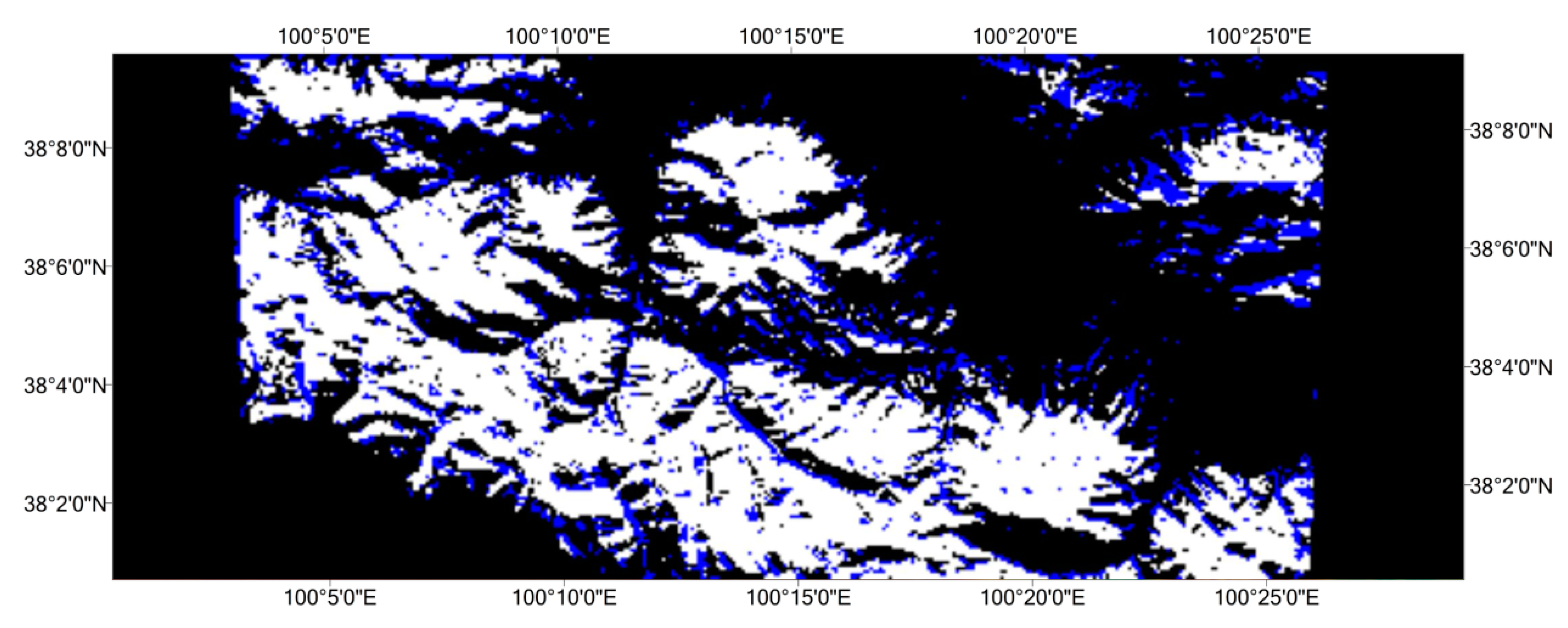
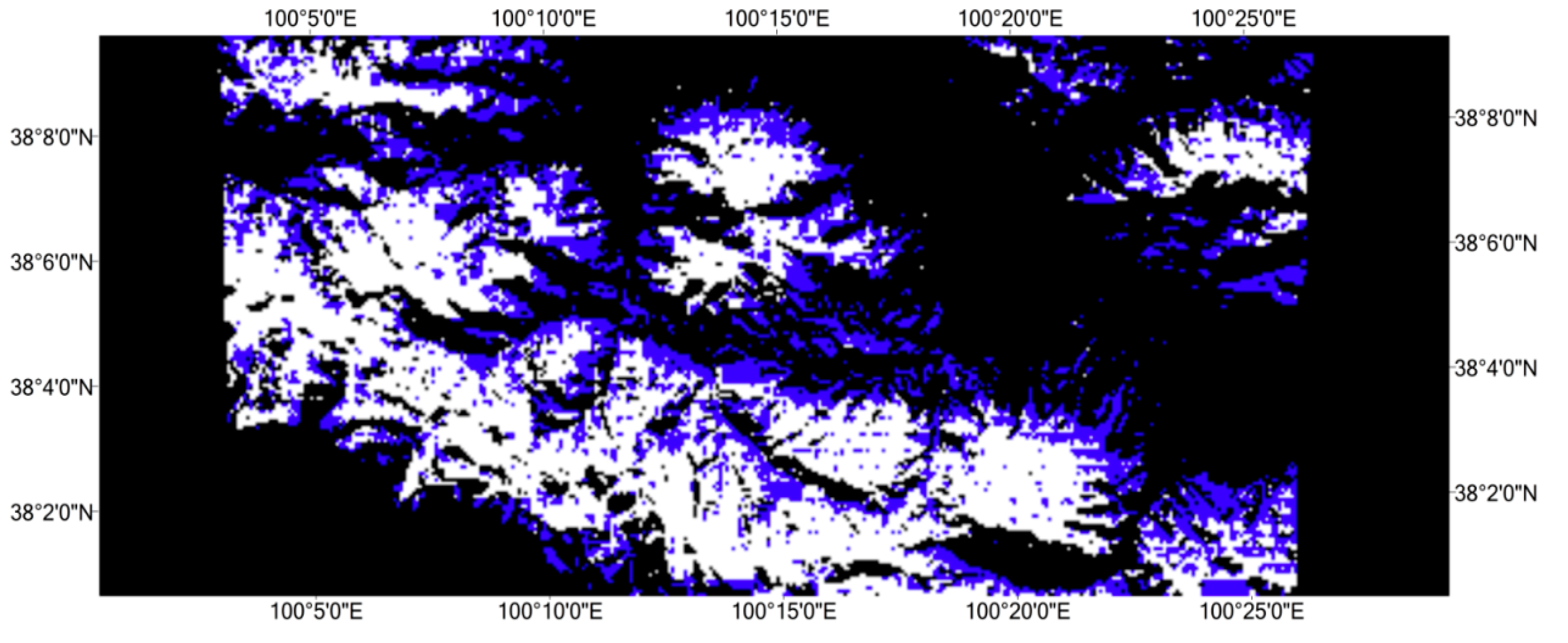
3.1. Remotely Sensed Snow Cover Data

3.1.1. Real Snow Distribution Maps Based on Multi-Source Remote Sensing Data

Multi-source remote sensing data are typically used to map snow cover patterns at different scales, including Landsat TM, CHRIS (Compact High Resolution Imaging Spectrometer), EO-1 (Earth Observing-1 Extended Mission) and MODIS. (Table 1). The Landsat 5 TM image data files consist of seven spectral bands which can supply snow classification using NDSI index method. 2 TM images with 30 m resolution are used in this paper. The TM data are from USGS (United State Geological Survey) archive. CHRIS was launched aboard Proba-1 satellite of ESA (European Space Agency) and provides hyperspectral images. 12 MODE 1 images from PROBA CHRIS are used in this study. Hyperion hyperspectral products from the EO-1 Extended Mission are used in this study. The spectral range of the EO-1 Hyperion data varies from 400 nm to 2500 nm. 4 EO-1 Hyperion images with 30 m resolution are collected in this study, which is from USGS Center. MODIS daily SCF data (MOD10A1) with resolution 500 m are obtained from NSIDC (National Snow and Ice Data Center).

Table 1. Remote sensing data used in this study.

Source	Number	Date		Resolution
PROBA/CHRIS	12	2008.11.18 2008.11.19 2009.01.10 2009.03.30 2009.03.31 2009.11.06	2009.11.14 2009.11.23 2009.11.24 2009.12.29 2010.01.07 2010.02.19	30 m
Landsat/EO-1	4	2008.03.17 2008.03.22	2008.03.27 2008.04.01	30 m
Landsat/TM	2	2008.03.17	2009.09.28	30 m
MODIS/Terra	18	All dates above		500 m

Table 1. Remote sensing data used in this study.

Source	Number	Date		Resolution
PROBA/CHRIS	12	2008.11.18 2008.11.19 2009.01.10 2009.03.30 2009.03.31 2009.11.06	2009.11.14 2009.11.23 2009.11.24 2009.12.29 2010.01.07 2010.02.19	30 m
Landsat/EO-1	4	2008.03.17 2008.03.22	2008.03.27 2008.04.01	30 m
Landsat/TM	2	2008.03.17	2009.09.28	30 m
MODIS/Terra	18	All dates above		500 m

CHRIS, EO-1 and TM data are preprocessed via radiometric calibration, atmospheric correction and geometric correction. Binary snow distributions are then mapped using these image data. Snow maps generated from these images are regarded as true snow distributions. The images with a 30-m resolution are used to validate the downscaled results, 16 SCF images are used as the training data, and the TM image in 17 March 2008 and EO-1 image in 27 March 2008 are used as independent evaluation data. MODIS SCF products are used to validate the method in case classification errors that are introduced in real SCF products.

For the TM and EO-1 data, the normalized difference snow index (NDSI) method is used to map snow distributions [34]. NDSI values are obtained using

$$NDSI=\frac{VIR-SIR}{VIR+SIR}$$

(8)

where VIR denotes the visible band reflectance, and SIR denotes the shortwave–infrared band reflectance. The NDSI method can detect snow distributions due to high reflectance in the visible band and high absorption in the shortwave–infrared band. When the pixel NDSI value exceeds a predefined criterion, the pixel is classified as snow covered. In certain regions, a criterion of 0.4 is adopted [34]. A previous study of the Qilian mountains showed that 0.36 best reflects snow classifications in this region [35].

The NDSI method is not suitable for use with CHRIS images because the spectral range of the CHRIS data (L1, MODE 1) varies from 773 nm to 1036 nm and lacks a shortwave–infrared band range (approximately 1500 nm), which is needed in the NDSI index method. In this study, binary snow distributions are mapped via supervised classification.

3.1.2. SCF Data

There are various means of retrieving SCF values from moderate-resolution satellite images such as MODIS data. Retrieval accuracy levels are influenced by various factors such as the reliability of the retrieval methods and atmospheric conditions. The accuracy of SCF values is somewhat uncertain. Because we focus here on the availability and reliability of the downscaled method, we minimize SCF errors using remotely sensed images with a resolution of 30 m to develop the SCF map with a resolution of 500 m. The 500-m resolution reflects the resolution of typical SCF products such as MODIS. The remotely sensed images with a resolution of 30 m included 18 CHRIS, TM and EO-1 images (see Table 1). Converting snow maps from a 30-m to a 500-m resolution involves three tasks.

(1)

Downscaling the 30-m-resolution binary snow map to a 10-m-resolution binary snow map via linear interpolation.

(2)

Counting the number of snow-covered grids in each region using 50 × 50 grids of the 10-m resolution binary snow map. Each region with 50 × 50 grids represents a 500-m-resolution grid.

(3)

Computing the snow-covered area in each 500-m-resolution grid to determine the 500-m-resolution SCF field.

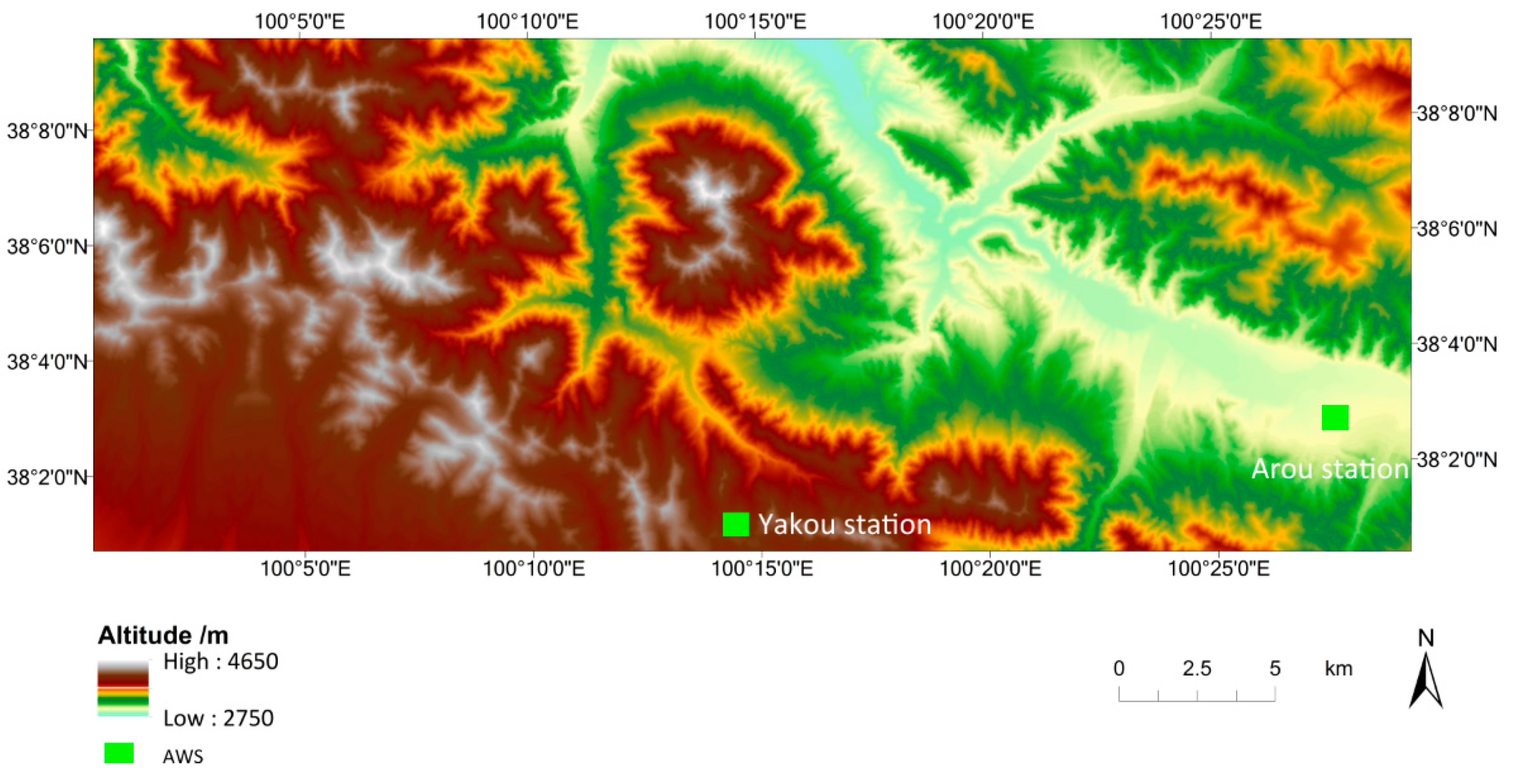
3.2. Study Region

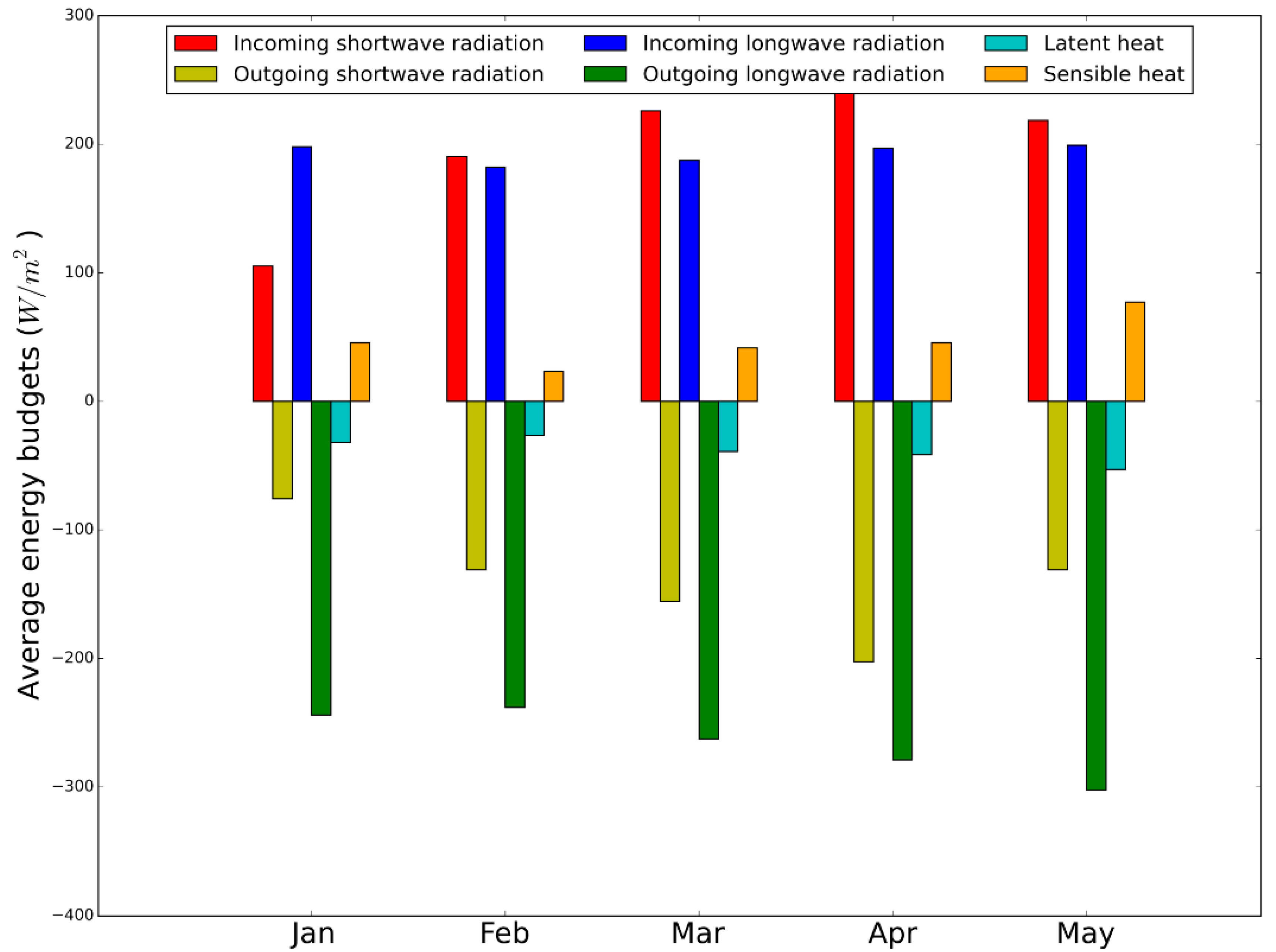
3.2.1. Topographic and Meteorological Data

The study area is located in the Babaohe basin of the Qilian mountains region in China [36]. The region covers an area of approximately 17.3 × 42.4 km (Figure 2). Two automatic weather stations (AWSs) are located in the study area: the Yakou station (4146 m, 100°14′E, 38°00′N) and the Arou station (2995 m, 100°27′E, 38°03′N). Our observations include hourly measurements of air temperature and solar radiation. The DEM is drawn from the World Data System for Cold and Arid Regions (http://data.westgis.ac.cn/) and has a resolution of 30 m [37,38]. The slope and aspect distributions are measured based on the DEM data.

Figure 2. Study region DEM and AWS locations in the Babaohe basin of the Qilian mountainous region in China. Two automatic weather stations are located in the study area.

Figure 2. Study region DEM and AWS locations in the Babaohe basin of the Qilian mountainous region in China. Two automatic weather stations are located in the study area.

Here a brief introduction about local energy budgets is made (Figure 3). The dataset used is from the previous study in this region [2]. Radiation data are from the weather station, and latent heat and sensible heat are from a physically based snow model. The period is from January to May 2008, which represents a typical snow season. In the station, incoming and outgoing shortwave radiation increases gradually from January to April, while incoming longwave radiation remains stable through the whole snow season but outgoing longwave radiation experiences a slow increase. Latent heat and sensible heat accounts for relatively small part.

3.2.2. Spatial Interpolation of Solar Radiation and Air Temperature

The observed AWS solar radiation is divided into direct and diffuse radiation; these values are distributed across the entire study region based on slope and aspect features. It is assumed that horizontal direct radiation is homogeneous throughout the study region because the region is relatively small. Here, we present a description of our solar radiation spatial interpolation method.

The atmospheric diffuse transmission coefficient (${\tau }_d$) is first calculated to divide the solar radiation into direct radiation and diffuse radiation [39,40,41]:

$${\tau }_d={\tau }_t\left[1-\exp \left(\frac{0.6(1-B/{\tau }_t)}{B-0.4}\right)\right]$$

(9)

where ${\tau }_d$ is the atmospheric diffuse transmission coefficient (S_diff/S_bo), S_diff is the diffuse radiation value, and S_bo is the total incident solar radiation on a horizontal surface along the outer edge of the atmosphere. Moreover, ${\tau }_t$ is the atmospheric total transmission coefficient (S_t/S_bo), and S_t is the AWS-observed incoming solar radiation, including both direct radiation S_dire and diffuse radiation S_diff. B is the maximum clear-sky transmissivity of the atmosphere, which is assumed to be 0.76 in this study.

Second, the diffuse and direct radiation are distributed across the entire study region using the following equations [42]:

$$S_{slope}=S_{dire}\cos Z+S_{diff\_slope}$$

(10)

$$S_{diff\_slope}=S_{diff}({\cos }^2{k}_s/2)+(1-{\cos }^2{k}_s/2){\alpha }_t{S}_{envi}$$

(11)

where S_slope is the solar radiation along a slope, and S_{diff_slope} is the diffuse radiation along a slope. Z is the incidence angle of the sun, which represents the angle between the solar beam and a line perpendicular to the snowpack surface. Ks is the slope. Moreover, $co{s}^2{k}_s/2$ represents the sky-view factor, and $1-co{s}^2{k}_s/2$ represents the fraction of the view from the slope that is occupied by the surrounding terrain. ${\alpha }_t$ is the albedo of the surrounding terrain, which is assumed to be 0.6 in this study. Furthermore, S_envi is the total shortwave flux density of the surrounding terrain. S_envi is seldom known directly; thus, S_dire is substituted as an approximation for S_envi in this study.

Normally, sufficient linearity exists between air temperature and elevation. The air temperature adiabatic lapse rate of two AWSs is first calculated. Then, spatial temperatures are determined based on the lapse rate and elevation difference in each study region grid.

Figure 3. Monthly energy budgets in Yakou station in the study region in the 2008 snow season.

Figure 3. Monthly energy budgets in Yakou station in the study region in the 2008 snow season.

4. Results

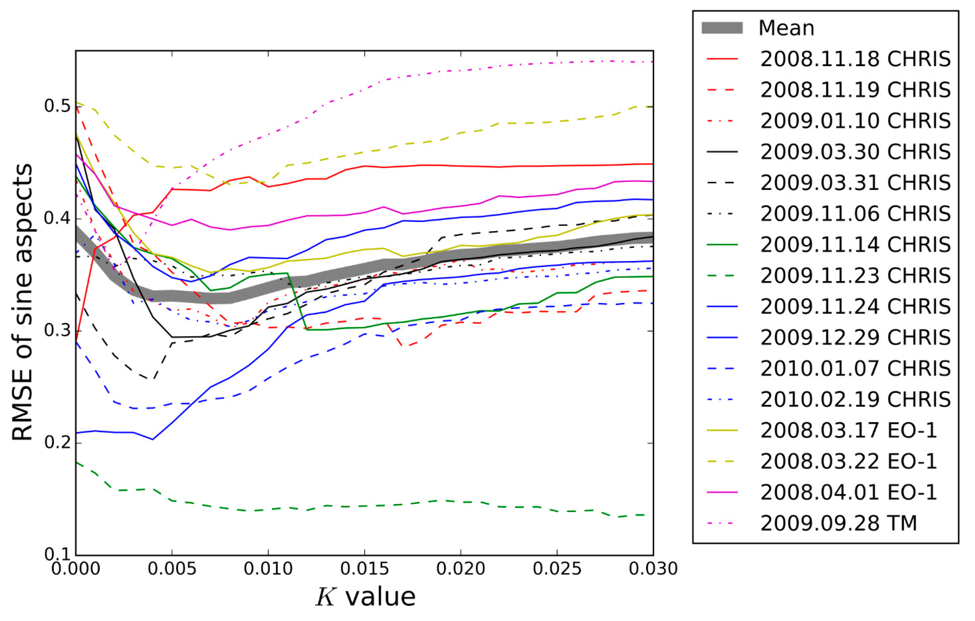
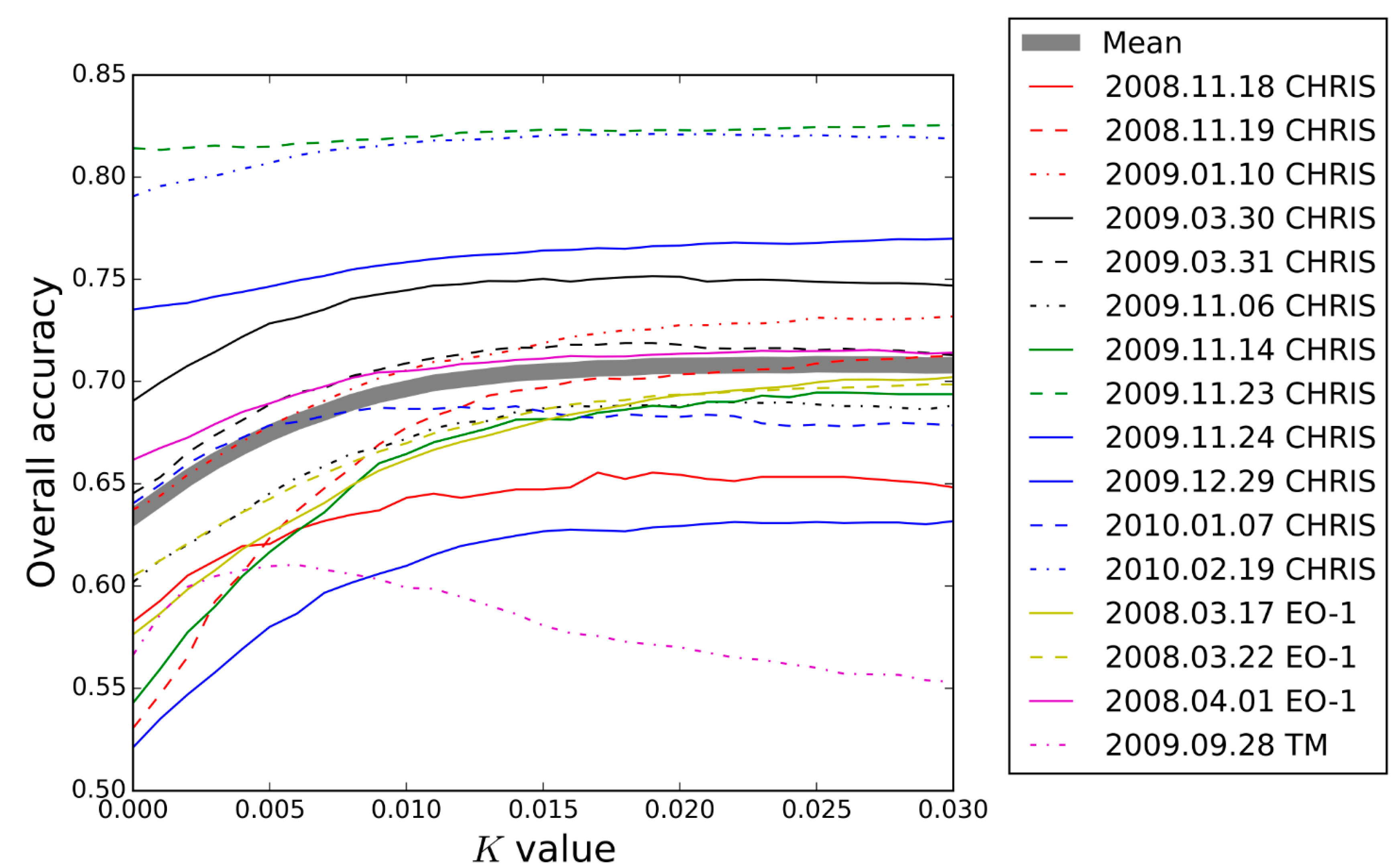
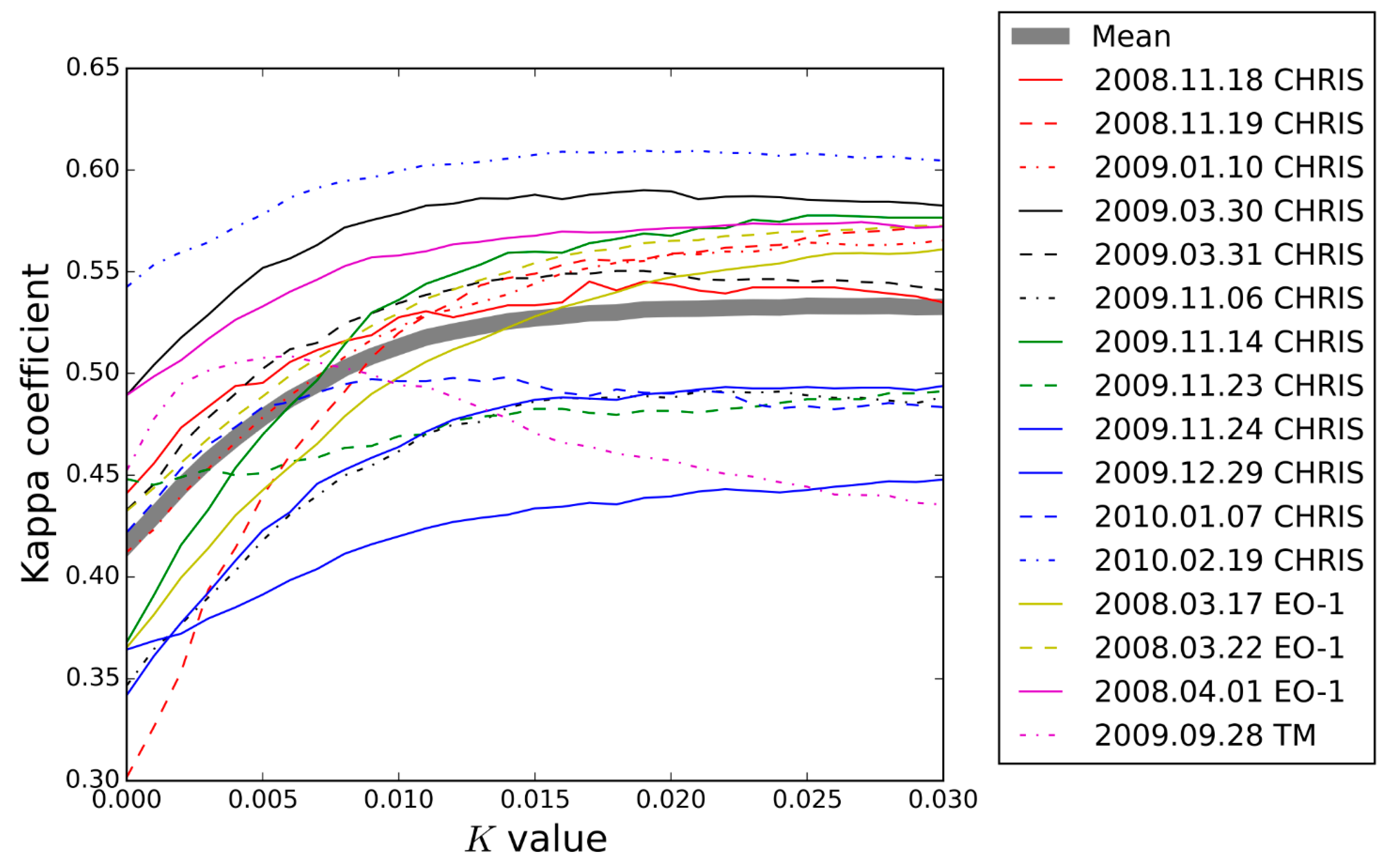
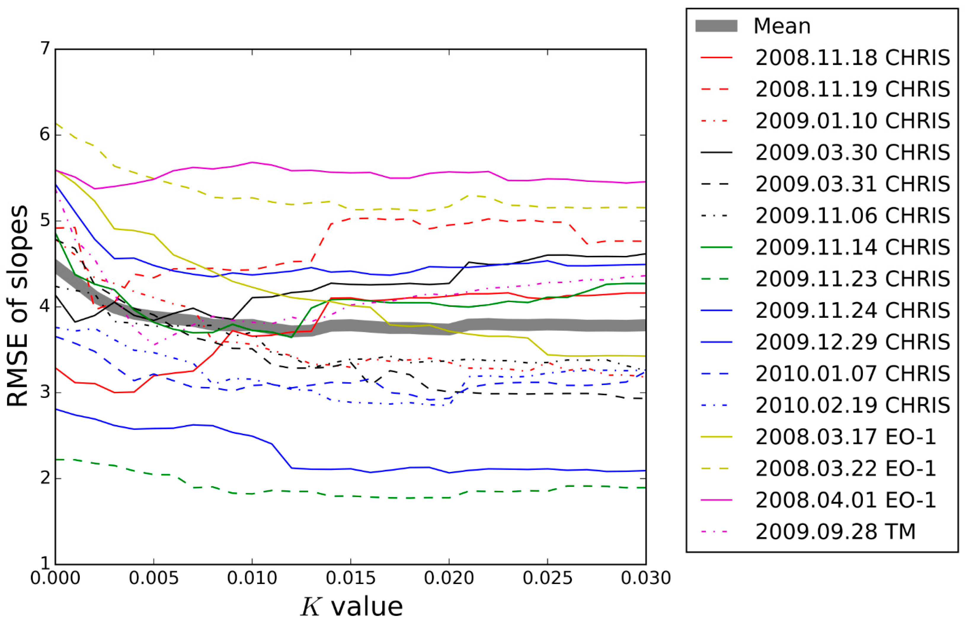
4.1. Determining K

We determine the accuracy of the downscaled snow maps based on the K values for various periods (Table 2) and find 0.009 to be the best value for the downscaled snow cover fraction data. We use 18 satellite images collected during the spring and winter snow seasons to verify the downscaling results based on different snow cover areas. The results indicate that this determined K value is stable during various periods in the study region.

Table 2. Mean downscaled snow map accuracies with different K values.

K Value	Mean Overall Accuracy	Mean Kappa Coefficient	Mean RMSE between the SLopes of DS and RS Subgrids (°)	Mean RMSE between the Sine of the Aspects of DS and RS Subgrids
0.000	0.63	0.42	4.5	0.388
0.001	0.64	0.43	4.3	0.370
0.002	0.65	0.44	4.1	0.349
0.003	0.66	0.46	4.0	0.337
0.004	0.67	0.47	3.9	0.331
0.005	0.67	0.48	3.9	0.332
0.006	0.68	0.49	3.9	0.330
0.007	0.68	0.49	3.8	0.329
0.008	0.69	0.50	3.8	0.329
0.009	0.69	0.51	3.8	0.330
0.010	0.70	0.51	3.8	0.339
0.011	0.70	0.52	3.7	0.343
0.012	0.70	0.52	3.7	0.344
0.013	0.70	0.52	3.7	0.349
0.014	0.70	0.53	3.8	0.352
0.015	0.70	0.53	3.8	0.356
0.016	0.71	0.53	3.8	0.359
0.017	0.71	0.53	3.8	0.359
0.018	0.71	0.53	3.8	0.362
0.019	0.71	0.53	3.7	0.366
0.020	0.71	0.53	3.7	0.368
0.021	0.71	0.53	3.8	0.369
0.022	0.71	0.53	3.8	0.372
0.023	0.71	0.53	3.8	0.372
0.024	0.71	0.53	3.8	0.374
0.025	0.71	0.53	3.8	0.375
0.026	0.71	0.53	3.8	0.377
0.027	0.71	0.53	3.8	0.380
0.028	0.71	0.53	3.8	0.381
0.029	0.71	0.53	3.8	0.383
0.030	0.71	0.53	3.8	0.383

Table 2. Mean downscaled snow map accuracies with different K values.

K Value	Mean Overall Accuracy	Mean Kappa Coefficient	Mean RMSE between the SLopes of DS and RS Subgrids (°)	Mean RMSE between the Sine of the Aspects of DS and RS Subgrids
0.000	0.63	0.42	4.5	0.388
0.001	0.64	0.43	4.3	0.370
0.002	0.65	0.44	4.1	0.349
0.003	0.66	0.46	4.0	0.337
0.004	0.67	0.47	3.9	0.331
0.005	0.67	0.48	3.9	0.332
0.006	0.68	0.49	3.9	0.330
0.007	0.68	0.49	3.8	0.329
0.008	0.69	0.50	3.8	0.329
0.009	0.69	0.51	3.8	0.330
0.010	0.70	0.51	3.8	0.339
0.011	0.70	0.52	3.7	0.343
0.012	0.70	0.52	3.7	0.344
0.013	0.70	0.52	3.7	0.349
0.014	0.70	0.53	3.8	0.352
0.015	0.70	0.53	3.8	0.356
0.016	0.71	0.53	3.8	0.359
0.017	0.71	0.53	3.8	0.359
0.018	0.71	0.53	3.8	0.362
0.019	0.71	0.53	3.7	0.366
0.020	0.71	0.53	3.7	0.368
0.021	0.71	0.53	3.8	0.369
0.022	0.71	0.53	3.8	0.372
0.023	0.71	0.53	3.8	0.372
0.024	0.71	0.53	3.8	0.374
0.025	0.71	0.53	3.8	0.375
0.026	0.71	0.53	3.8	0.377
0.027	0.71	0.53	3.8	0.380
0.028	0.71	0.53	3.8	0.381
0.029	0.71	0.53	3.8	0.383
0.030	0.71	0.53	3.8	0.383

The mean overall accuracy is found to be 0.69, and the mean kappa coefficient is 0.51, i.e., the maximum corresponding to a K of 0.009. The mean RMSE of snow covered slopes between the downscaled snow map and the real snow map is found to be 3.9°, and the mean RMSE of the sine of the now covered aspects is found to be 0.34, which is equivalent to 19.9° (Table 2). The highest overall accuracy is 0.71 when K exceeds 0.015 (Figure 4). The optimal kappa coefficient is 0.53, which is stable for values of K exceeding 0.014 (Figure 5). The minimum RMSE of the simulated slope is 3.8° when K reaches approximately 0.012 (Figure 6). The RMSE of the sine of the aspect reaches a minimum of 0.335, which is equivalent to 19.6°, while K is approximately 0.007 (Figure 7). Rather than using only one index such as the overall accuracy or kappa coefficient, the four indexes should be considered together when determining the best K coefficient value. A value of 0.009 effectively mitigates the variations in the indexes. When K is 0.009, the overall accuracy is 0.69, which is close to the best value of 0.71, and the kappa coefficient is 0.51, which is close to the best value of 0.53. The RMSEs for the simulated slope and sine of the aspect are close to the minimum values.

We also note variations in downscaling accuracy due to different K values.

(1)

In this study, air temperature and solar radiation differences are understood to affect inhomogeneous snow distributions at the subgrid scale. Temperature differences at different elevations may play a dominant role in causing inhomogeneities. Solar radiation associated with various slopes and aspects has a secondary role.

When K reaches zero, according to Equation (1), only air temperature differences are used to determine the potential snow ablation capacities. The kappa coefficient ranges from 0.30 to 0.55, with a mean value of 0.42 (Figure 5). With an increase in K, the role of solar radiation becomes greater, and the kappa coefficient reaches a stable value that ranges from 0.43 to 0.61, with a mean value of 0.53. The results indicate an increase in the kappa coefficient from 0.42 to 0.53 when solar radiation is considered, indicating that downscaling accuracy levels can be marginally improved when solar radiation is considered.

(2)

In determining K values, the accuracy of the downscaled aspect plays a more important role than the slope. When K is zero, the RMSEs between the slopes in different downscaled images range from 2.2° to 6.8°, with an average value of 4.7°; as K increases, the RMSE gradually decreases to a stable value with an average of 3.8°. The RMSEs for the sine of the aspect followed a different trend than those for the slopes, i.e., decreasing to minimum values and then increasing gradually. When K is zero, the RMSEs for the sine of the aspect range from 0.18 to 0.55, with an average of 0.40; when K is 0.007, the average RMSE reaches a minimum of 0.33. Thereafter, the RMSE gradually increases to 0.39. When K exceeds 0.014, the kappa coefficient and slope accuracy of the downscaled results exhibit no further improvement, and the aspect accuracy worsens. Thus, the accuracy of the aspect should be considered a decisive factor when determining K values when the slope and kappa coefficient accuracies become stable.

Overall, using a single assessment criterion may skew downscaled snow cover fraction data. The method based on four indicators used in this study can yield downscaled snow distributions that agree well with the real distributions.

Figure 4. Overall accuracies of downscaled maps with various K values. High-resolution satellite images are used to verify the downscaling results based on different snow cover areas. Each line represents an accuracy change due to the adjustment of the K value. Accuracy changes have a similar trend with increasing K value.

Figure 4. Overall accuracies of downscaled maps with various K values. High-resolution satellite images are used to verify the downscaling results based on different snow cover areas. Each line represents an accuracy change due to the adjustment of the K value. Accuracy changes have a similar trend with increasing K value.

Figure 5. Kappa coefficients for the downscaled snow maps with different K values. High-resolution satellite images are used as the ground truth. It indicates similar trends of Kappa coefficients with increased K value between different calibration processes.

Figure 5. Kappa coefficients for the downscaled snow maps with different K values. High-resolution satellite images are used as the ground truth. It indicates similar trends of Kappa coefficients with increased K value between different calibration processes.

Figure 6. The RMSEs between the slopes of the downscaled snow covered subgrids and real snow covered subgrids for different K values.

Figure 6. The RMSEs between the slopes of the downscaled snow covered subgrids and real snow covered subgrids for different K values.

Figure 7. RMSE between the sine of the aspects of the downscaled snow covered subgrids and real snow covered subgrids.

Figure 7. RMSE between the sine of the aspects of the downscaled snow covered subgrids and real snow covered subgrids.

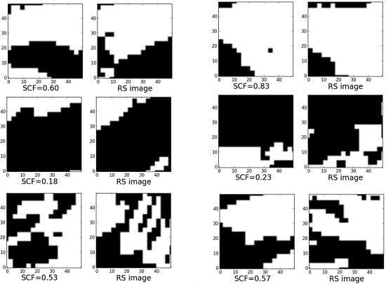
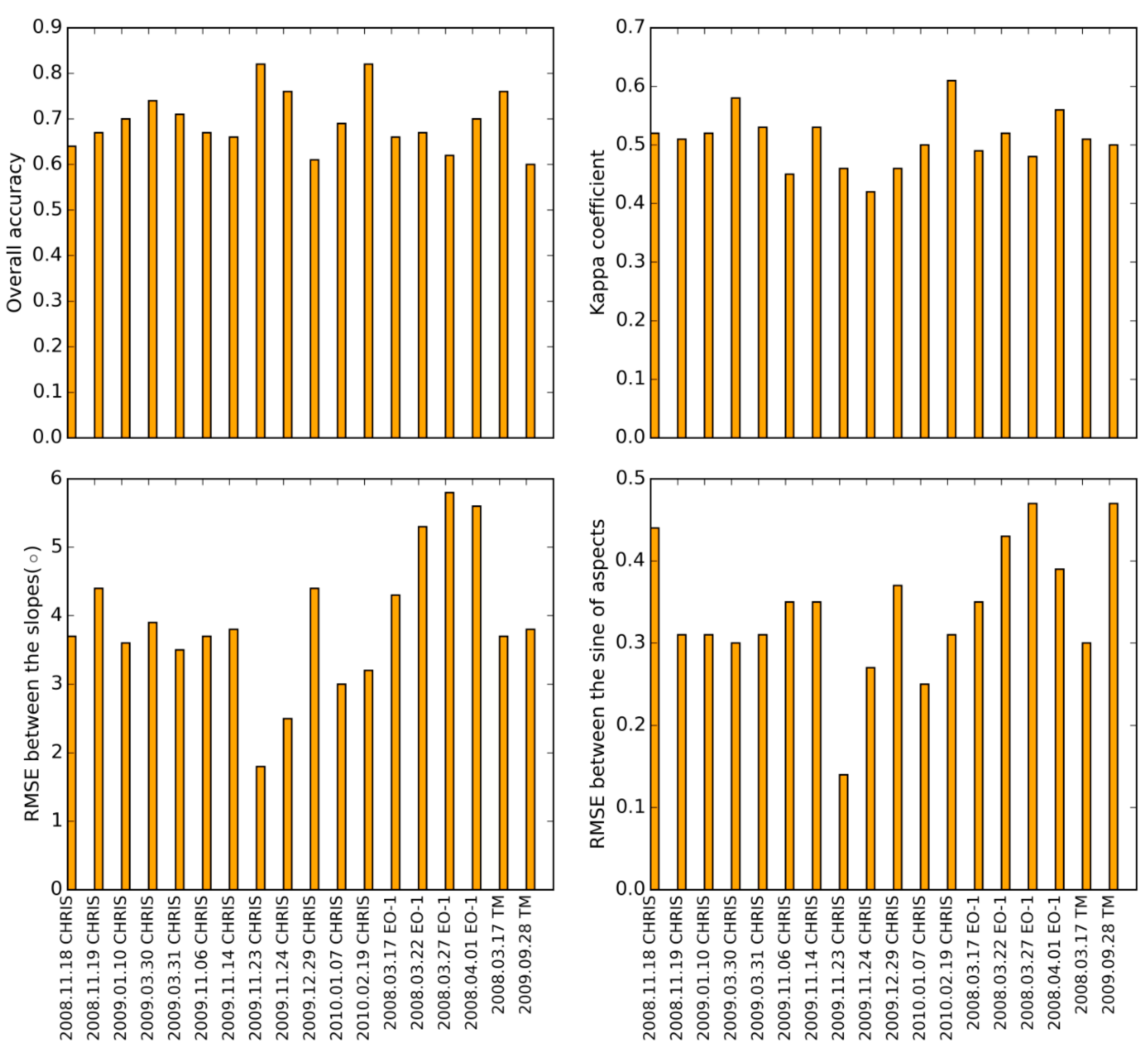
4.2. Downscaled Snow Map Accuracy Assessment

In this work, remotely sensed 30-m-resolution snow maps are used to verify the downscaled snow map. The results reveal good agreement between the downscaled map and the real results (Figure 8). The highest and lowest overall accuracies are 0.82 and 0.60, respectively, with a mean of 0.69. The maximum and minimum RMSEs of the slopes are 5.8° and 1.8°, respectively, with an average of 3.9°. The maximum and minimum RMSEs for the sine of the aspects are 0.47 and 0.14, respectively, with an average of 0.34, which is equivalent to 19.9°.

Figure 8. Accuracies of the downscaled snow map for different periods assuming K is 0.009. The X-coordinate is different image sources. For example, “2008.11.18 CHRIS” means the snow map from CHRIS data in 18 November 2008. The Y-coordinates are overall accuracy, kappa coefficient, RMSE between the slopes of real high-resolution snow map and downscaled snow map and RMSE between the sine of aspects of real high-resolution snow map and downscaled snow map.

Figure 8. Accuracies of the downscaled snow map for different periods assuming K is 0.009. The X-coordinate is different image sources. For example, “2008.11.18 CHRIS” means the snow map from CHRIS data in 18 November 2008. The Y-coordinates are overall accuracy, kappa coefficient, RMSE between the slopes of real high-resolution snow map and downscaled snow map and RMSE between the sine of aspects of real high-resolution snow map and downscaled snow map.

The downscaled snow map is fairly accurate. The snow-covered areas approximate the real snow distributions. Below, we present downscaled pixel-scale snow maps (Figure 9). The differences indicate that the topographic features of the snow distribution are well reproduced. We present an example to illustrate the spatial agreement between the downscaled snow map and the real trends (Figure 10). The misclassified area is located primarily along the boundaries of the snow-covered area.

Figure 9. Differences between downscaled snow pixels and 30-m-resolution RS images. Six comparisons are presented. The figure on the left is the downscaled snow map generated for a known SCF, and the figure on the right is the real snow distribution. Snow-covered and snow-free areas are depicted in white and black, respectively.

Figure 9. Differences between downscaled snow pixels and 30-m-resolution RS images. Six comparisons are presented. The figure on the left is the downscaled snow map generated for a known SCF, and the figure on the right is the real snow distribution. Snow-covered and snow-free areas are depicted in white and black, respectively.

Figure 10. Differences between the high-resolution downscaled and remotely sensed snow maps for 17 March 2008. Snow-free areas and areas lacking data are shown in black in both maps; snow-covered areas in the remotely sensed map that were identified as being snow-free in the downscaled map are blue; and snow-covered regions in both maps are white.

Figure 10. Differences between the high-resolution downscaled and remotely sensed snow maps for 17 March 2008. Snow-free areas and areas lacking data are shown in black in both maps; snow-covered areas in the remotely sensed map that were identified as being snow-free in the downscaled map are blue; and snow-covered regions in both maps are white.

5. Discussion

5.1. Applicability of the Downscaled Method Driven by Air Temperature and Solar Radiation

In a given region, snow distribution patterns are similar from one year to the next due to the presence of similar topographical conditions and weather patterns [31]. Topographic conditions affect meteorological factors and contribute to snow ablation. Meteorological conditions are an underlying cause of inhomogeneous snow ablation. In this study, air temperature and solar radiation are examined as two major determinants of meteorological conditions. Previous studies have also recommended using air temperature and solar radiation to simulate snow ablation patterns in areas of complex terrain [28,43].

We use an empirical linear formula that combines air temperature and solar radiation to simulate snow ablation patterns. The K parameter is used to adjust the contributions of air temperature and solar radiation to ablation. It is assumed that K is stable and independent of topographic conditions. Our results indicate that this is a viable assumption. Moreover, we use satellite images taken during different seasons to verify the downscaled results with different K values. Similar features are observed regardless of the K value selected during the calibration; hence, a constant of 0.009 is used as the final calibrated K value. The results indicate that a single K constant could satisfy the downscaled accuracies of snow maps.

If a more complex, physically based snow model can better simulate snow distribution heterogeneity, can one obtain superior downscaled results? Generally, physically based snow models are more accurate than empirical models, assuming the former’s use of precise data. Moreover, the physically based snow model takes into account more physical processes without neglecting regional parameters [44]. However, precise large-scale data regarding wind speeds, humidity and longwave radiation are difficult to obtain. The accuracy of modeled snow ablation depends primarily on meteorological forcing data, which are controlled by topographic differences. Previous studies have found that solar radiation and air temperature are more accurate than wind speed and precipitation [45]. When using more-complex models, more uncertainties are introduced due to the use of more data. In certain cases, complex models may not yield the best results [43]. In regions of scarce data, such as sparsely gauged mountainous regions, we suggest that empirical methods based on air temperature and solar radiation are the most appropriate for downscaling snow fraction data.

5.2. Limitations of the Downscaling Method and Error Analysis

Our results suggest that the downscaling method employed in this study is reasonable. However, the method is limited in terms of its accuracy (i.e., an overall accuracy of 0.71 is the highest level recorded).

5.2.1. Spatial Scale Limit

Snow distribution patterns vary at different spatial scales [46]. At macro-scales, i.e., 10 to 1,000 km, snow distribution patterns depend on latitude, elevation and orography. At mesoscales, with linear distances of 100 m to 1000 m, snow deposition and accumulation patterns may be related to elevation, slope, aspect, and vegetation cover. Moreover, at microscales, i.e., 10 to 100 m, accumulation patterns are primarily controlled by surface roughness conditions. The method presented in this paper is found to be suitable for application at the mesoscale. Topographic features are the main factors in our interpolation study of meteorological data, as discussed in Section 3.2.2. Macroscale and microscale snow-distribution mechanisms differ greatly from those at the mesoscale due to the presence of different applicable conditions.

Based on the above considerations, the downscaled method presented in this paper is suitable for satellite images of 500- to 1000-m resolution.

5.2.2. Errors due to an Absence of Blowing Snow and Inhomogeneous Precipitation

Air temperature and solar radiation are examined as two dominant factors that can be used to downscale snow fraction data at the 500-m scale. Although blowing snow is not considered in this study, it can disturb the accuracy of downscaled results in certain regions.

While blowing snow may have affected our downscaled results, it is not likely to have exerted a major effect. Blowing snow only affects high-altitude regions characterized by high wind speeds. In extreme cases, blowing snow can continuously redistribute snow in certain regions. This process challenges the assumption made in this study that air temperature and solar radiation are the two dominant factors. In these cases, errors due to blowing snow cannot be ignored. In the study region, blowing snow weather patterns typically occur under dry snow conditions in the winter at altitudes exceeding 4000 m [47]. Blowing snow patterns decline sharply at altitudes below 3700 m. Blowing snow patterns are not significant in our study region; thus, a good agreement is obtained without considering blowing snow in this study. However, if this method is to be applied in other regions, an evaluation of blowing snow conditions would be necessary.

Several sophisticated methods have been used to model blowing snow [48,49]. These methods have revealed complex processes of blowing snow mass exchange. However, these methods require access to precise wind flow simulations and snow properties, which are difficult to obtain, especially in cold regions. This is one reason why only solar radiation and air temperature are considered in this study.

The inhomogeneous precipitation can also affect the heterogeneity of snow ablation. The heterogeneity is more obvious on a large spatial scale. In this study, 500-m resolution is used as the grid scale, and it is assumed the heterogeneity from precipitation is not the dominant factor resulting in the inhomogeneous snow ablation in this scale. This assumption needs more detailed field observations as proof. Microtopography and inhomogeneous wind speed both can affect the spatial distribution of precipitation. In particular, the influence from blowing snow needs to be distinguished between from precipitation. Because there are only two weather stations in the study region, it is not enough to give a reliable analysis in the spatial heterogeneity of precipitation. The topic is indeed very important, though, and detailed field observations are needed to examine it.

5.2.3. Errors in the Employed Data

In addition to errors of the downscaled method, data errors must also be noted.

Remote sensing image identification errors cannot be ignored. As noted above, due to uncertainties in terms of the accuracy of SCF products, more reliable datasets should be used. We downscaled the MODIS fractional snow cover data (MOD10A1) to snow locations at a subgrid scale using the same method and parameters. The downscaled results and accuracies are compared with the previous results using SCF data calculated from high-resolution images such as TM, EO-1 and CHRIS. We present two diagrams to show the results (Figure 11 and Figure 12). Three conclusions are drawn from the results.

(1)

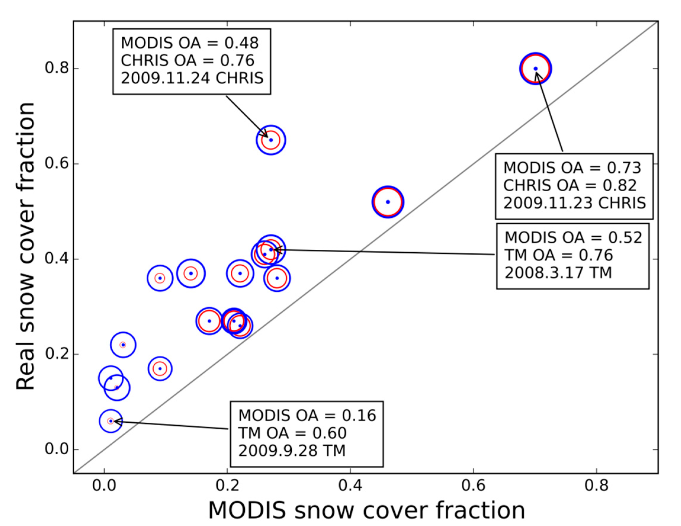
MODIS SCF products yield systematic underestimation, as shown in Figure 11. The SCF values across the region of different dates are compared with the “real” SCF obtained from high-resolution satellite images. Our results indicate that the underestimation occurs primarily where the snow cover fraction is relatively low and at lower elevations (Figure 12). Other studies in this region mentioned similar results. For example, Zhang et al. [50] reported that the SCF in the MODIS standard product is less than the “ground truth” obtained from ETM+ images with 30-m resolution, and the MODIS product fails to retrieve snow in the snow cover-transition areas with patchy snow. Rittger et al. [51] found that the MODIS SCF product is slightly underestimated in the Himalaya region. Fortunately, a few previous studies have generated strong retrieval results. For example, an improved endmember extraction method was employed to improve fractional snow cover mapping in our study region [50]. This method is based on the fast autonomous spectral endmember determination (N-FINDR) maximizing volume iteration algorithm and on orthogonal subspace projection theory. For MODIS data, the study reported a retrieved RMSE for the SCF of 0.14, which is superior to that of the MODIS standard fractional snow cover product (MOD10A1) [50]. Because this paper focuses on the downscaling method, we only analyze the influence of errors from MODIS standard products (MOD10A1) in the downscaling accuracy and do not involve other SCF products using different retrieval methods.

(2)

As expected, the errors from the MODIS product reduce the downscaled accuracy. The accuracy of the MODIS SCF is better, and the downscaled accuracy is closer to the best value using high-resolution images. For example (Figure 11), on 23 November 2009, the MODIS SCF of the study region is 0.70 and the CHRIS SCF is 0.80, whereas the overall accuracy (OA) of the downscaled snow map from the MODIS SCF product is 0.73 and the OA using CHRIS is 0.82. Both calculation results and accuracies are close. By contrast, on 24 November 2009, the MODIS SCF of the study region is 0.27 and the CHRIS SCF is 0.65, whereas the OA of the downscaled snow map using the MODIS product is 0.48 and the OA using CHRIS is 0.76. There is a large difference between the accuracies because the MODIS product dramatically underestimates the SCF value on that day. Overall, better accuracy of the MODIS SCF leads to better downscaling accuracy because there is less error in the MODIS product itself.

(3)

We also find that a higher SCF is related to higher downscaling accuracy of the MODIS products. For example, on 28 September 2009, the MODIS SCF of the study region is 0.01 and the CHRIS SCF is 0.06, whereas the OA of the downscaled snow map using the MODIS product is 0.16 and the OA using the TM is 0.60. In this case, the SCFs from MODIS and TM are close; however, the downscaled results different substantially. The underlying cause is still the misestimation associated with the MODIS SCF products in low-SCF regions, as mentioned earlier.

In general, reliable downscaling accuracy can be obtained where the errors in the MODIS SCF products are low using the method presented in this paper. The downscaling results are better particularly where the snow cover area is large. The underestimation produced by the MODIS SCF products can seriously reduce the downscaling accuracy, especially in regions with small areas of snow cover. Retrieval errors must be considered in future studies based on the downscaled method.

Figure 11. Comparison between MODIS snow cover fraction and the real snow cover fraction retrieved from high-resolution satellite images such as TM, CHRIS and EO-1 images. The radius of a blue circle represents the overall accuracy (OA) of a downscaled snow map based on high-resolution satellite images, and the radius of a red circle represents that of a downscaled map based on MODIS SCF products. For clarity, four annotations are presented in the figure: OAs of downscaled snow maps based on TM and CHRIS data are compared with those of MODIS products.

Figure 11. Comparison between MODIS snow cover fraction and the real snow cover fraction retrieved from high-resolution satellite images such as TM, CHRIS and EO-1 images. The radius of a blue circle represents the overall accuracy (OA) of a downscaled snow map based on high-resolution satellite images, and the radius of a red circle represents that of a downscaled map based on MODIS SCF products. For clarity, four annotations are presented in the figure: OAs of downscaled snow maps based on TM and CHRIS data are compared with those of MODIS products.

Figure 12. Differences between the MODIS-based downscaled and remotely sensed snow maps for 17 March 2008. Snow-free areas and areas lacking data are shown in black in both maps; snow-covered areas in the remotely sensed map that were identified as being snow-free in the downscaled map are blue; and snow-covered regions in both maps are white. This image can be compared with the downscaled snow map based on high-resolution images shown in Figure 10.

Figure 12. Differences between the MODIS-based downscaled and remotely sensed snow maps for 17 March 2008. Snow-free areas and areas lacking data are shown in black in both maps; snow-covered areas in the remotely sensed map that were identified as being snow-free in the downscaled map are blue; and snow-covered regions in both maps are white. This image can be compared with the downscaled snow map based on high-resolution images shown in Figure 10.

We used an empirical method using air temperature and solar radiation as inputs to approximately simulate the heterogeneity of snow ablation at subgrid scale. The method uses a simplification to represent all energy budgets. Obviously its accuracy is less than the complex physically based snow model which clearly consider different energy budgets such as longwave radiation and turbulent fluxes. The main reason for using the empirically method in this paper is the data availability and accuracy, as we discussed in Section 5.1. The solar radiation and air temperature distributions are interpolated based on station observations and DEM data. Given the complexities of mountainous weather patterns, some data may be inaccurate, especially data from areas far from the stations. Investigators should carefully examine the applicability of the downscaled method in these regions when using other data sources, such as reanalyzed atmospheric forcing data, instead of data from local stations. Vegetation conditions also affect snow accumulation patterns. Our study region is almost uniformly covered with grassland; thus, we do not consider potential effects of inhomogeneous vegetation distributions. A previous study also mentioned the possible influence of forest in snow classification in downscaling snow maps [20]. If this method is generalized to other regions, we recommend the study of smaller areas due to potential meteorological data errors and inhomogeneous vegetation patterns. Large study areas may be divided into smaller regions, and SCF data can be downscaled for each separate region.

In this study, some river ice is classified as snow. Although we use prior information regarding river channel locations to identify river ice in the snow map, in some higher-elevation areas, river ice and snow are not easily distinguishable. The river ice formation mechanism differs significantly from that of snow and does not depend primarily on topographic features and temperatures, which leads to errors in the downscaled snow distribution. Fortunately, these areas are small.

6. Conclusions

A simple and reliable method is used to downscale snow cover fraction data in a mountainous region. The downscaled snow map shows good agreement with the real snow distribution. The mean overall accuracy is 0.69 for all 18 remotely sensed images. The applicability of the downscaled method based on air temperature, solar radiation, sources of error and means of methodological improvement is discussed above. The following conclusions can be drawn from this work:

(1)

The downscaled method is suitable for reconstructing subgrid-scale snow distributions. Slope and aspect information for snow-covered areas can be retrieved with sufficient accuracy compared to the real information. Downscaled results may be used in hydrological simulations or in other studies that require more accurate snow distribution data.

(2)

This method can be applied to other similar mountainous regions. A spatial scale of 500 m is employed herein. Because most remotely sensed snow map products employ kilometer-based resolutions, the method can be used for such products (e.g., MODIS data). Only air temperature, solar radiation and DEM data are required. This simplicity ensures the applicability of this method to sparsely gauged mountainous regions.

(3)

Spatial scales must be considered when this method is generalized to other similar regions due to the different mechanisms that are important for snow distributions, data interpolation errors and vegetation heterogeneities. Blowing snow should be considered in areas where such patterns are prominent. If sophisticated physically based snow processes are considered while employing downscaling methods, the accuracy of the data should remain intact.

References

- Li, X.; Cheng, G.D.; Jin, H.J.; Kang, E.S.; Che, T.; Jin, R.; Wu, L.Z.; Nan, Z.T.; Wang, J.; Shen, Y.P. Cryospheric change in China. Glob. Planet. Chang. 2008, 62, 210–218. [Google Scholar] [CrossRef]
- Li, H.Y.; Wang, J. Simulation of snow distribution and melt under cloudy conditions in an Alpine watershed. Hydrol. Earth Syst. Sci. 2011, 15, 2195–2203. [Google Scholar] [CrossRef]
- Qin, D.; Liu, S.; Li, P. Snow cover distribution, variability, and response to climate change in Western China. J. Clim. 2006, 19, 1820–1833. [Google Scholar]
- Cline, D.W.; Bales, R.C.; Dozier, J. Estimating the spatial distribution of snow in mountain basins using remote sensing and energy balance modeling. Water Resour. Res. 1998, 34, 1275–1285. [Google Scholar] [CrossRef]
- Yang, D.; Gao, B.; Jiao, Y.; Lei, H.; Zhang, Y.; Yang, H.; Cong, Z. A distributed scheme developed for eco-hydrological modeling in the upper Heihe River. Sci. China Earth Sci. 2015, 58, 36–45. [Google Scholar] [CrossRef]
- Dozier, J. A clear-sky spectral solar radiation model for snow-covered mountainous terrain. Water Resour. Res. 1980, 16, 709–718. [Google Scholar] [CrossRef]
- Hall, D.K.; Tait, A.B.; Foster, J.L.; Chang, A.T.C.; Allen, M. Intercomparison of satellite-derived snow-cover maps. Ann. Glaciol. 2000, 31, 369–376. [Google Scholar] [CrossRef]
- Czyzowska-Wisniewski, E.H.; van Leeuwen, W.J.D.; Hirschboeck, K.K.; Marsh, S.E.; Wisniewski, W.T. Fractional snow cover estimation in complex alpine-forested environments using an artificial neural network. Remote Sens. Environ. 2015, 156, 403–417. [Google Scholar] [CrossRef]
- Yang, J.; Jiang, L.; Ménard, C.B.; Luojus, K.; Lemmetyinen, J.; Pulliainen, J. Evaluation of snow products over the Tibetan Plateau. Hydrol. Process. 2015. [Google Scholar] [CrossRef]
- Rosenthal, W.; Dozier, J. Automated mapping of montane snow cover at subpixel resolution from the Landsat Thematic Mapper. Water Resour. Res. 1996, 32, 115–130. [Google Scholar] [CrossRef]
- Wang, J.; Li, H.X.; Hao, X.H.; Huang, X.D.; Hou, J.L.; Che, T.; Dai, L.Y.; Liang, T.G.; Huang, C.L.; Li, H.Y.; et al. Remote sensing for snow hydrology in China: Challenges and perspectives. J. Appl. Remote Sens. 2014, 8, 084687. [Google Scholar] [CrossRef]
- Arsenault, K.R.; Houser, P.R.; de Lannoy, G.J.M. Evaluation of the MODIS snow cover fraction product. Hydrol. Process. 2012, 28, 980–998. [Google Scholar] [CrossRef]
- Salomonson, V.V.; Appel, I. Estimating fractional snow cover from MODIS using the normalized difference snow index. Remote Sens. Environ. 2004, 89, 351–360. [Google Scholar] [CrossRef]
- Painter, T.H.; Rittger, K.; McKenzie, C.; Slaughter, P.; Davis, R.E.; Dozier, J. Retrieval of subpixel snow covered area, grain size, and albedo from MODIS. Remote Sens. Environ. 2009, 113, 868–879. [Google Scholar] [CrossRef]
- Homan, J.W.; Luce, C.H.; McNamara, J.P.; Glenn, N.F. Improvement of distributed snowmelt energy balance modeling with MODIS-based NDSI-derived fractional snow-covered area data. Hydrol. Process. 2011, 25, 650–660. [Google Scholar] [CrossRef]
- Zhang, G.Q.; Xie, H.J.; Yao, T.D.; Liang, T.G.; Kang, S.C. Snow cover dynamics of four lake basins over Tibetan Plateau using time series MODIS data (2001–2010). Water Resour. Res. 2012, 48, W10529. [Google Scholar] [CrossRef]
- Gao, Y.; Xie, H.; Lu, N.; Yao, T.; Liang, T. Toward advanced daily cloud-free snow cover and snow water equivalent products from Terra-Aqua MODIS and Aqua AMSR-E measurements. J. Hydrol. 2010, 385, 23–35. [Google Scholar] [CrossRef]
- Gafurov, A.; Bárdossy, A. Cloud removal methodology from MODIS snow cover product. Hydrol. Earth Syst. Sci. 2009, 13, 1361–1373. [Google Scholar] [CrossRef]
- Hall, D.K.; Riggs, G.A.; Foster, J.L.; Kumar, S.V. Development and evaluation of a cloud-gap-filled MODIS daily snow-cover product. Remote Sens. Environ. 2010, 114, 496–503. [Google Scholar] [CrossRef]
- Walters, R.D.; Watson, K.A.; Marshall, H.P.; McNamara, J.P.; Flores, A.N. A physiographic approach to downscaling fractional snow cover data in mountainous regions. Remote Sens. Environ. 2014, 152, 413–425. [Google Scholar] [CrossRef]
- Skaugen, T.; Randen, F. Modeling the spatial distribution of snow water equivalent, taking into account changes in snow-covered area. Ann. Glaciol. 2013, 54, 305–313. [Google Scholar] [CrossRef]
- Marchand, W.D.; Killingtveit, A. Statistical probability distribution of snow depth at the model sub-grid cell spatial scale. Hydrol. Process. 2005, 19, 355–369. [Google Scholar] [CrossRef]
- Liston, G.E. Representing subgrid snow cover heterogeneities in regional and global models. J. Clim. 2004, 17, 1381–1397. [Google Scholar] [CrossRef]
- Luce, C.H.; Tarboton, D.G. The application of depletion curves for parameterization of subgrid variability of snow. Hydrol. Process. 2004, 18, 1409–1422. [Google Scholar] [CrossRef]
- Kolberg, S.A.; Gottschalk, L. Updating of snow depletion curve with remote sensing data. Hydrol. Process. 2006, 20, 2363–2380. [Google Scholar] [CrossRef]
- Hebeler, F.; Purves, R.S. The influence of resolution and topographic uncertainty on melt modelling using hypsometric sub-grid parameterization. Hydrol. Process. 2008, 22, 3965–3979. [Google Scholar] [CrossRef] [Green Version]
- Liston, G.E.; Elder, K. A meteorological distribution system for high-resolution terrestrial modeling (MicroMet). J. Hydrometeorol. 2006, 7, 217–234. [Google Scholar] [CrossRef]
- Brubaker, K.; Rango, A.; Kustas, W. Incorporating radiation inputs into the snowmelt runoff model. Hydrol. Process. 1996, 10, 1329–1343. [Google Scholar] [CrossRef]
- Cazorzi, F.; Dalla Fontana, G. Snowmelt modelling by combining air temperature and a distributed radiation index. J. Hydrol. 1996, 181, 169–187. [Google Scholar] [CrossRef]
- Molotch, N.P.; Margulis, S.A. Estimating the distribution of snow water equivalent using remotely sensed snow cover data and a spatially distributed snowmelt model: A multi-resolution, multi-sensor comparison. Adv. Water Resour. 2008, 31, 1503–1514. [Google Scholar] [CrossRef]
- Sturm, M.; Wagner, A.M. Using repeated patterns in snow distribution modeling: An Arctic example. Water Resour. Res. 2010, 46, W12549. [Google Scholar] [CrossRef]
- Cohen, J. A coefficient of agreement for nominal scales. Educ. Psychol. Meas. 1960, 20, 37–46. [Google Scholar] [CrossRef]
- Landis, J.R.; Koch, G.G. The measurement of observer agreement for categorical data. Biometrics 1977, 33, 159–174. [Google Scholar] [CrossRef] [PubMed]
- Hall, D.K.; Riggs, A.; Salomonson, V.V. Development of methods for mapping global snow cover using moderate resolution imaging spectroradiometer data. Remote Sens. Environ. 1995, 54, 127–140. [Google Scholar] [CrossRef]
- Hao, X.; Wang, J.; Li, H.Y. Evaluation of the NDSI threshold value in mapping snow cover of MODIS—A case study of snow in the Middle Qilian Mountains. J. Glaciol. Geocryol. 2008, 30, 132–138. [Google Scholar]
- Li, X.; Cheng, G.; Liu, S.; Xiao, Q.; Ma, M.; Jin, R.; Che, T.; Liu, Q.; Wang, W.; Qi, Y.; et al. Heihe Watershed Allied Telemetry Experimental Research (HiWATER): Scientific objectives and experimental design. Bull. Am. Meteorol. Soc. 2013, 94, 1145–1160. [Google Scholar] [CrossRef]
- Cheng, G.; Li, X. Integrated research methods in watershed science. Sci. China Earth Sci. 2015, 58, 1159–1168. [Google Scholar] [CrossRef]
- Cheng, G.; Li, X.; Zhao, W.; Xu, Z.; Feng, Q.; Xiao, S.; Xiao, H. Integrated study of the water-ecosystem-economy in the Heihe River Basin. Natl. Sci. Rev. 2014, 1, 413–428. [Google Scholar] [CrossRef]
- Flerchinger, G.N. The Simultaneous Heat and Water (SHAW) Model. Available online: http://www.ars.usda.gov/SP2UserFiles/Place/20520000/ShawDocumentation.pdf (accessed on 4 May 2015).
- Xiao, W.; Flerchinger, G.N.; Yu, Q.; Zheng, Y.F. Evaluation of the SHAW model in simulating the components of net all-wave radiation. Trans. ASABE 2006, 49, 1351–1360. [Google Scholar] [CrossRef]
- Bristow, K.L.; Campbell, G.S.; Saxton, K.E. An equation for separating daily solar irradiation into direct and diffuse components. Agric. For. Meteorol. 1985, 35, 123–131. [Google Scholar] [CrossRef]
- DeWalle, D.R.; Rango, A. Principles of Snow Hydrology; Cambridge University Press: Cambridge, UK, 2008. [Google Scholar]
- Valéry, A.; Andréassian, V.; Perrin, C. “As simple as possible but not simpler”: What is useful in a temperature-based snow-accounting routine? Part 1—Comparison of six snow accounting routines on 380 catchments. J. Hydrol. 2014, 517, 1166–1175. [Google Scholar] [CrossRef]
- Bartlett, S.J.; Lehning, M. A theoretical assessment of heat transfer by ventilation in homogeneous snowpacks. Water Resour. Res. 2011, 47, W04503. [Google Scholar] [CrossRef]
- Pan, X.; Tian, X.; Li, X.; Xie, Z.; Shao, A.; Lu, C. Assimilating Doppler radar radial velocity and reflectivity observations in the weather research and forecasting model by a proper orthogonal-decomposition-based ensemble, three-dimensional variational assimilation method. J. Geophys. Res. 2012, 117, D17113. [Google Scholar] [CrossRef]
- Gray, D.M.; Prowse, T.D. Snow and floating ice. In Handbook of Hydrology; Maidment, D.R., Ed.; MCGRAW-HILL Professional: New York, NY, USA, 1993; pp. 259–304. [Google Scholar]
- Li, H.; Wang, J.; Hao, X. Role of blowing snow in snow processes in Qilian Mountainous region. Sci. Cold Arid Reg. 2014, 6, 124–130. [Google Scholar]
- Fang, X.; Pomeroy, J.W. Modelling blowing snow redistribution to prairie wetlands. Hydrol. Process. 2009, 23, 2557–2569. [Google Scholar] [CrossRef]
- Bowling, L.C.; Pomeroy, J.W.; Lettenmaier, D.P. Parameterization of blowing-snow sublimation in a macroscale hydrology model. J. Hydrometeorol. 2004, 5, 745–762. [Google Scholar] [CrossRef]
- Zhang, Y.; Huang, X.; Hao, X.; Wang, J.; Wang, W.; Liang, T. Fractional snow-cover mapping using an improved endmember extraction algorithm. J. Appl. Remote Sens. 2014, 8, 084691:1–084691:11. [Google Scholar] [CrossRef]
- Rittger, K.; Painter, T.H.; Dozier, J. Assessment of methods for mapping snow cover from MODIS. Adv. Water Resour. 2013, 51, 367–380. [Google Scholar] [CrossRef]
© 2015 by the authors; licensee MDPI, Basel, Switzerland. This article is an open access article distributed under the terms and conditions of the Creative Commons Attribution license (http://creativecommons.org/licenses/by/4.0/).
Share and Cite
Li, H.Y.; He, Y.Q.; Hao, X.H.; Che, T.; Wang, J.; Huang, X.D. Downscaling Snow Cover Fraction Data in Mountainous Regions Based on Simulated Inhomogeneous Snow Ablation. Remote Sens. 2015, 7, 8995-9019. https://doi.org/10.3390/rs70708995
Li HY, He YQ, Hao XH, Che T, Wang J, Huang XD. Downscaling Snow Cover Fraction Data in Mountainous Regions Based on Simulated Inhomogeneous Snow Ablation. Remote Sensing. 2015; 7(7):8995-9019. https://doi.org/10.3390/rs70708995
Chicago/Turabian StyleLi, Hong Yi, Yong Qi He, Xiao Hua Hao, Tao Che, Jian Wang, and Xiao Dong Huang. 2015. "Downscaling Snow Cover Fraction Data in Mountainous Regions Based on Simulated Inhomogeneous Snow Ablation" Remote Sensing 7, no. 7: 8995-9019. https://doi.org/10.3390/rs70708995