A Robust Algorithm of Multiquadric Method Based on an Improved Huber Loss Function for Interpolating Remote-Sensing-Derived Elevation Data Sets

Abstract

Remote-sensing-derived elevation data sets often suffer from noise and outliers due to various reasons, such as the physical limitations of sensors, multiple reflectance, occlusions and low contrast of texture. Outliers generally have a seriously negative effect on DEM construction. Some interpolation methods like ordinary kriging (OK) are capable of smoothing noise inherent in sample points, but are sensitive to outliers. In this paper, a robust algorithm of multiquadric method (MQ) based on an Improved Huber loss function (MQ-IH) has been developed to decrease the impact of outliers on DEM construction. Theoretically, the improved Huber loss function is null for outliers, quadratic for small errors, and linear for others. Simulated data sets drawn from a mathematical surface with different error distributions were employed to analyze the robustness of MQ-IH. Results indicate that MQ-IH obtains a good balance between efficiency and robustness. Namely, the performance of MQ-IH is comparative to those of the classical MQ and MQ based on the Classical Huber loss function (MQ-CH) when sample points follow a normal distribution, and the former outperforms the latter two when sample points are subject to outliers. For example, for the Cauchy error distribution with the location parameter of 0 and scale parameter of 1, the root mean square errors (RMSEs) of MQ-CH and the classical MQ are 0.3916 and 1.4591, respectively, whereas that of MQ-IH is 0.3698. The performance of MQ-IH is further evaluated by qualitative and quantitative analysis through a real-world example of DEM construction with the stereo-images-derived elevation points. Results demonstrate that compared with the classical interpolation methods, including natural neighbor (NN), OK and ANUDEM (a program that calculates regular grid digital elevation models (DEMs) with sensible shape and drainage structure from arbitrarily large topographic data sets), and two versions of MQ, including the classical MQ and MQ-CH, MQ-IH has a better ability of maximally reducing the impact of outliers, while faithfully preserving terrain features. Theoretically, MQ-IH is not a promising interpolation method, and some side effects can be found from its simulation results. For example, the contours of MQ-IH are coarser than ANUDEM in some locations of the real-world study site, and its hill shade may not strictly agree with the real-world surface at rough terrain. Furthermore, the computing cost of MQ-IH is much bigger than that of the classical interpolation methods. However, compared with the classical interpolation methods, MQ-IH has significant potential for interpolating remote-sensing-derived elevation data sets.

1. Introduction

At present, remote-sensing techniques have been widely adopted to capture DEM data sources, such as Light Detection and Ranging (LiDAR), Interferometric Synthetic Aperture Radar (InSAR) and photogrammetry [1,2,3]. However, due to the physical limitations of sensors, multiple reflectance, occlusions and low contrast of texture, remote-sensing-derived elevation data sets always suffer from outliers [4,5,6,7]. In a statistical sense, a spatial outlier is an observation whose value is significantly inconsistent with those of its spatial neighbors [8,9]. The existence of outliers seriously affects subsequent spatial data analyses and often distorts the inference process. In principle, if the uncertainties of sample data are known, then the outliers can be tested based on prior knowledge. However, this is a non-trivial task. It has been demonstrated that the uncertainties of sample points are highly dependent on the landscapes of the study areas [10,11], and the attributes of the scanner and the scanner geometry, such as distance and surface orientation [12,13].

Diagnostic and robust statistics are two different branches that deal with the problem of outliers. In the context of DEM construction with diagnostic statistics, outliers are first detected and removed, and then the traditional interpolation methods are used to interpolate the remaining data [4,14,15]. Compared with diagnostic statistics, robust statistics have great potential to be resilient to outliers, which is stable with respect to small changes in the data, and even large changes in the underlying data pattern cannot cause a complete failure of the procedures [16,17]. Theoretically, a perfect robust interpolation method is capable of maximally resisting the effect of outliers, while faithfully constructing terrain surfaces. In this paper, we only focus on the development of robust interpolation methods.

Presently, many promising algorithms have been proposed for generating DEMs, such as natural neighbor (NN), ordinary kriging (OK), and Multiquadric method (MQ) [18,19,20]. A series of tests indicated that MQ can be considered as an excellent interpolation method in terms of timing, storage, accuracy, visual pleasantness of the surface, and ease of implementation [21,22]. However, the classical MQ is an exact interpolator and sensitive to outliers due to its sum of squared error loss function.

In the theory of statistics, the Huber loss function has been widely applied to robust regression, which reduces the effect of outliers on parameter estimation, while treating non-outliers in a more standard way [23]. The Huber loss function considers a convex differentiable cost function, which is quadratic for small errors and linear for others. However, the classical Huber loss function does not completely avoid the effect of outliers, since its influence function is a constant for points with very large errors (i.e., outliers). Therefore, the objectives of this paper are to: (1) develop a robust algorithm of MQ method based on an Improved Huber loss function (MQ-IH) that is completely resist the impact of outliers; (2) test the robustness of MQ-IH to outliers for surface modeling with simulated data sets subject to errors with different distributions; and (3) compare the performance of MQ-IH with those of the classical interpolation methods, including natural neighbor (NN), ordinary kriging (OK), ANUDEM and the classical MQ for DEM construction with stereo-images-derived elevation data set.

The remainder of this paper is organized as follows. Section 2 presents a short literature review for diagnostic and robust statistics. Section 3 gives the principle and procedure of MQ-IH for interpolations. In Section 4, a numerical test for surface modeling with five groups of simulated data sets is first employed to assess the robustness of MQ-IH, and then a real-world example for DEM construction with stereo-images-derived elevation data set is used to compare the performance of MQ-IH with those of the classical interpolation methods. Discussion and conclusions are provided in Section 5 and Section 6, respectively.

2. Related Works

Many methods related to outlier detection have been explored in different disciplines, like statistics and geosciences. In statistics, the existing traditional outlier detection algorithms can be classified into the following five categories, clustering-based, distribution-based, depth-based, density-based and distance-based. For clustering-based approaches, the major data cluster distributions are found and the points that do not belong to any cluster are defined as outliers [24,25]. Distribution-based approaches employ a standard distribution (e.g., Gaussian and Laplacian) to fit the data set, so that data points with heavy deviations from this distribution are defined as outliers [9]. Depth-based methods organize the data in different layers of k-dimensional convex hulls, where the data in the outer layers are defined as outliers [26,27]. Density-based approaches define the outlier with the analysis of data distribution density, which uses a local outlier factor (LOF) to compare the density of each data with those of its neighbors [28]. Thus, the data with a higher LOF is considered an outlier. Distance-based methods use a distance metric to measure the relationship between data samples and define the data as an outlier, which is obviously far away from the other data [29,30]. Generally, the aforementioned methods for detecting outliers mainly focus on low dimensional and non-spatial data sets [31].

In geosciences, the methods for spatial outlier detection can be generally classified into two categories, graphic approaches and quantitative tests. Graphic approaches to outlier detection are mostly based on visualizing spatial data [32]. Podobnikar [33] defined four classes of visual methods for assessing the accuracy of DTMs: visualizations according to spatial analytical operations based on one or multiple datasets; visualizations according to spatial statistical analysis; non-spatial visualizations; and other visualization techniques/other algorithms. Additionally, scatterplot and Moran scatterplot are two representative visualization approaches [34,35]. However, the scatterplot approaches are ineffective when sample points have huge data volumes and contain several outliers. Thus, many researchers have focused on the development of quantitative methods for outlier detection. For example, Liu, et al. [4] presented a method to find outliers mixed in remote-sensing-derived elevation points in terms of some sensitive outlier indices and locally adaptive and robust statistical criteria. Lu, et al. [27] proposed a set of graph-based algorithms to identify spatial outliers in US housing and Census data. Nevertheless, when several outliers cluster together, they could mask the effect of one another by increasing the size of residuals for other observations. This is the well-known masking and swapping problem. Yet, this problem can be overcome by the method based on Mahalanobis distance and Minimum Covariance Determinant (MCD). For example, Chen, et al. [31] used this method to detect spatial outliers with single and multiple attributes in West Nile virus data set. Giménez, et al. [36] employed this method to detect multivariate outliers in the processing of RTK positions. Nurunnabi, et al. [37] proposed a diagnostic principle component analysis (PCA) for dealing with mobile LiDAR point clouds, where the outliers are detected and removed with the robust Mahalanobis distance. It should be noted that the performance of Mahalanobis distance-based method is not assured for surface modeling of DEMs in areas with complex terrain characteristics, since it only depends on a simple linear interpolation to determine the neighborhood relationship in the process of outlier detection.

In principle, the robust interpolation methods resist the effect of outliers on surface modeling based on robust loss functions. In various disciplines including computer vision, computer graphics, computational geometry and robotics, different robust methods have been explored for plane surface fitting. For instance, Fleishman, et al. [38] proposed a forward-search-based robust moving least squares technique for reconstructing piecewise smooth surfaces. The random sample consensus (RANSAC) algorithm, presented by Fischler and Bolles [39], has been frequently optimized and generalized for decreasing the effect of outliers on planar surface fitting [40,41,42]. Debese, et al. [43] developed a robust fitting method of polynomial based on M-estimator for multibeam echosounder data interpolation. Nurunnabi, et al. [6] developed two robust versions of PCA with robust covariance [44] and Projection Pursuit [45] for planar surface fitting. However, the aforementioned methods are simple linear interpolators, which is ineffective in simulating steep slope areas.

Therefore, in order to avoid the shortcomings of the aforementioned methods, a promising robust interpolation method is developed in this paper, which combines the advantages of the nonlinear interpolation method (i.e., MQ) for dealing with complex terrain surfaces, and an improved Huber loss function for decreasing the effect of outliers on surface modeling.

3. Proposed Robust Algorithm

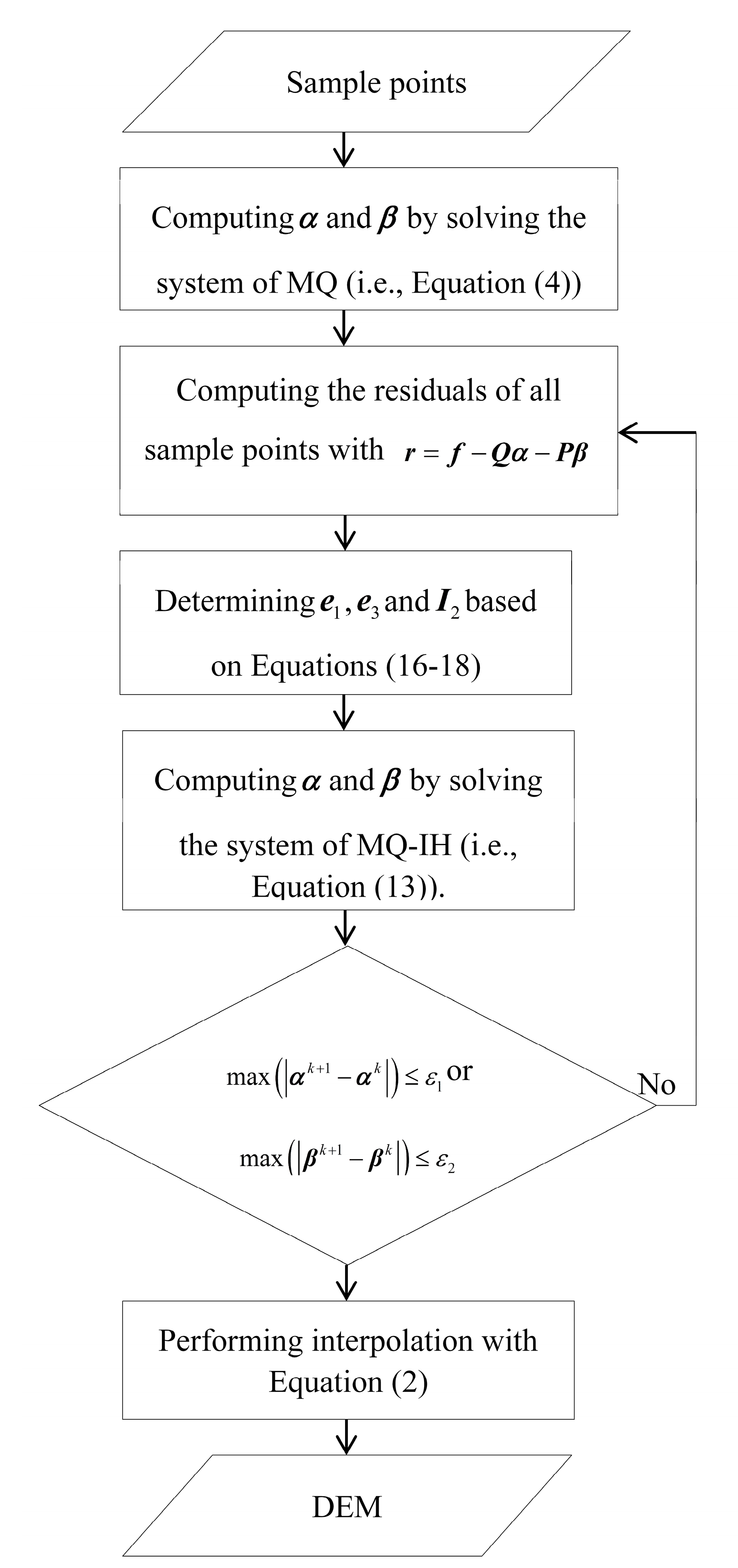
In data analysis, the essential framework of smoothing divides the observations into two components including signal and noise. Smoothing interpolation attempts to recover the coherent signal and remove noise, simultaneously. The general smoothing model can be expressed as [46],

$$\left[z(x_i,y_i)=f(x_i,y_i)+e(x_i,y_i),i=1,2,\cdots ,n\right]$$

(1)

where f(x_i, y_i) is the value of a smoothing function to be modeled based on the sample point z(x_i, y_i), which includes the sample error e(x_i, y_i); n is the number of sample points.

Multiquadric method (MQ) is an analytical interpolator of representing irregular surfaces that involve the summation of equations of quadric surfaces located at significant topographic points. In terms of MQ, the smoothing function f(x, y) is expressed as [47],

$$\left[f(x,y)={\displaystyle \sum _{j=1}^n{\alpha }_{j}q(r_j)}+{\displaystyle \sum _{j=0}^m{\beta }_j{p}_j(x,y)}\right]$$

(2)

where m is the degree of the polynomial; p_j(x, y) and β_j are the jth basis and coefficient of the polynomial; r_j is the distance from the interpolated point (x, y) to the jth data point; q(r) and α, respectively, represent a basis function and its weight. For MQ,

$$\left[q\left(r\right)=\sqrt{r^2+c^2}\right]$$

(3)

where c is a shape parameter. Its optimal value depends on the number and the distribution of data points, on the data vector and on the precision of the computation [48,49].

In order to perform interpolations with MQ (i.e., Equation (2)), the variables α and β must be computed. From Appendix A, we can obtain that,

$$\left[\{\begin{array}{c}\alpha =L^{-1}\left(I-P{N}^{-1}{P}^T{L}^{-1}\right)f\\ \beta =N^{-1}{P}^T{L}^{-1}\text{f\hspace{0.05em}\hspace{0.05em}\hspace{0.05em}\hspace{0.05em}\hspace{0.05em}\hspace{0.05em}\hspace{0.05em}\hspace{0.05em}\hspace{0.05em}\hspace{0.05em}\hspace{0.05em}\hspace{0.05em}\hspace{0.05em}\hspace{0.05em}\hspace{0.05em}\hspace{0.05em}\hspace{0.05em}\hspace{0.05em}\hspace{0.05em}\hspace{0.05em}\hspace{0.05em}\hspace{0.05em}\hspace{0.05em}\hspace{0.05em}\hspace{0.05em}\hspace{0.05em}\hspace{0.05em}}\end{array}\right]$$

(4)

where

$$L=Q+\lambda I$$

(5)

$$N=P^T{L}^{-1}P$$

(6)

$$Q=\left[\begin{array}{ccc}{q}_{11}& \cdots & q_{1n}\\ ⋮& \ddots & ⋮\\ q_{n1}& \cdots & q_{nn}\end{array}\right]$$

(7)

$$P=\left[\begin{array}{ccc}{p}_{11}& \cdots & p_{1m}\\ ⋮& \ddots & ⋮\\ p_{n1}& \cdots & p_{nm}\end{array}\right]$$

(8)

$$q_{ij}=q\left(r_{ij}\right)$$

(9)

$$p_{ij}=p_j(x_i,y_i)$$

(10)

λ is a positive real constant, which determines the relative importance of loss function and the weight regularization term. In the case of noisy data, one avoids overfitting by taking a smaller λ value.

It can be concluded from Appendix A that the classical MQ is inherently sensitive to outliers due to the least squares loss function in the objective function. In statistical theory, the Huber loss function has been widely applied to robust regression, which reduces the effect of outliers on parameter estimation, while treating non-outliers in a more standard way [23]. However, the Huber loss function cannot completely resist the effect of outliers due to the influence function of points with large residuals being a constant. Hence, an improved version is developed in this paper. It is expressed as follows,

$$\left[L_{\epsilon }(r)=\{\begin{array}{c}0,A_0=\left\{r|r/s>c_2\right\}\\ c_1\left(r/s-c_1/2\right),A_1=\left\{r|c_1\le r/s\le c_2\right\}\\ {\left(r/\sqrt{2}s\right)}^2,A_2=\left\{r|-c_1\le r/s<c_1\right\}\\ -c_1\left(r/s+c_1/2\right),A_3=\left\{r|-c_2\le r/s<-c_1\right\}\\ 0,A_4=\left\{r|r/s<-c_2\right\}\end{array}\right]$$

(11)

where s is the standard deviation of simulation residuals; c₁ and c₂ represent two constants, which are typically set as c₁ = 2.5 and c₂ = 3. This is a reasonable selection taking into account the fact that for a Gaussian distribution in statistics, there are only a few residuals bigger than 2.5 s [14]. In order to improve the robustness and efficiency of s, we used the scale estimator of Rousseeuw and Croux [50], which is expressed as,

$$\left[s=1.1926{\text{med}}_i\left\{{\text{med}}_j\left|v_i-v_j\right|\right\}\right]$$

(12)

where med_i(x) is the median of x. As Rousseeuw and Croux mentioned in their paper [50], this scale estimator has 50% breakdown point and 58% Gaussian efficiency, whereas median absolute deviation only has 37% Gaussian efficiency.

In this article, we assume that the spatial data sets under investigation are observations on a spatially continuous geospatial variable. These types of geospatial variables show gradual and continuous variation over space, and can be represented as a surface. Hence, if a point has a large simulation residual during surface modeling, we consider it as an outlier. Equation (11) indicates that the improved Huber loss function is null for large errors, and therefore completely avoids the impact of outliers.

Taking Equation (11) as the loss function in the objective function of MQ-IH, we can obtain α and β as follows (Appendix B),

$$\left[\{\begin{array}{c}\alpha ={\widehat{L}}^{-1}\left(I-I_{2}P{\widehat{N}}^{-1}{P}^T{\widehat{L}}^{-1}\right)\left(I_{2}f+c_1{e}_1-c_1{e}_3\right)\\ \beta \text{\hspace{0.05em}\hspace{0.05em}=}{\widehat{N}}^{-1}{P}^T{\widehat{L}}^{-1}\left(I_{2}f+c_1{e}_1-c_1{e}_3\right)\end{array}\right]$$

(13)

where

$$\widehat{L}=\lambda I+I_{2}Q$$

(14)

$$\widehat{N}{P}^T{\widehat{L}}^{-1}{I}_{2}P$$

(15)

$$\left[{\left(\underset{n\times 1}{e_1}\right)}_i=\{\begin{array}{c}1,r_i\in A_1\\ 0,others\end{array}\right]$$

(16)

$$\left[{\left(\underset{n\times 1}{e_3}\right)}_i=\{\begin{array}{c}1,r_i\in A_3\\ 0,others\end{array}\right]$$

(17)

$$\left[{\left(\underset{n\times n}{I_2}\right)}_{i,i}=\{\begin{array}{c}1,r_i\in A_2\\ 0,others\end{array}\right]$$

(18)

the other expressions can be found in Equations (7–10).

Comparing Equation (4) with Equation (13), we can find that Equation (4) is a special case of Equation (13) with I₂ being the identity matrix, and all the elements of e₁ and e₃ being zeroes. Namely, for the classical MQ, the residuals of all sample points belong to the set A₂.

The procedure of MQ-IH (Figure 1) for carrying out robust interpolations is as follows:

Figure 1. Flow chart of MQ-IH for carrying out interpolations.

Figure 1. Flow chart of MQ-IH for carrying out interpolations.

(1)

Solving the linear systems of the classical MQ method (i.e., Equation (4)) to obtain α and β. The parameter λ is pre-determined by the k-fold cross-validation (e.g., k = 10) technique [51].

(2)

Computing the residuals of all sample points with r = f − Qα − Pβ.

(3)

Determining e₁, e₃ and I₂ based on Equations (16–18).

(4)

Computing α and β based on Equation (13).

(5)

Repeating 2–4 until either max(|α^k+1 − α^k|) or max(|β^k+1 − β^k|) is smaller than a pre-set tolerance. In this paper, the pre-set tolerance is set as 0.01.

(6)

Carrying out interpolations with Equation (2).

4. Experimental Verification

In our experimental verification, a numerical test and a real-world test were, respectively, employed to assess the performance of MQ-IH for surface modeling and for DEM construction. In the numerical test, we validated the robustness of MQ-IH and MQ based on the classical Huber loss function (MQ-CH) to outliers for surface modeling, and these results were compared with the classical MQ. In the real-world example, we compared the performance of MQ-IH with those of the classical interpolation methods including NN, OK and ANUDEM, and the two versions of MQ, including the classical MQ and MQ-CH for DEM construction with stereo-images-derived elevation data set.

4.1. Numerical Test

A mathematical surface (Figure 2) was employed as the test surface to analyze the robustness of MQ-IH, so that the “true” output value can be pre-determined to avoid uncertainty caused by uncontrollable data errors. The mathematical surface has the following formulation:

$$\left[\begin{array}{l}z(x_i,y_i)=3{(1-x_i)}^2\exp (-x_i^2-{(y_i+1)}^2)-10(0.2x_i-x_i^3-y_i^5)\exp (-x_i^2-y_i^2)\\ -\frac{1}{3}\exp (-{(x_i+1)}^2-y_i^2)+r_i,i=1,2,\cdots ,n\end{array}\right]$$

(19)

where r_i is the model error of the ith sample point (x_i, y_i); n is the number of sample points.

Figure 2. The mathematical surface in the numerical test.

Figure 2. The mathematical surface in the numerical test.

In the numerical tests, the model errors r_i(i = 1, 2, …, n) were, respectively, drawn from one of the following distributions:

Case 1: the normal distribution N (0, 1) with the mean of 0 and the standard deviation of 1.

Case 2: the contaminated normal distribution (1 − θ) × N (0, 1) + θ × N (0, 5²), where θ is the contaminating proportion, which is, respectively, taken as 10%, 20% and 30%.

Case 3: the Cauchy distribution C (0, 1) with the location parameter of 0 and scale parameter of 1.

In principle, if model errors were drawn from the normal distribution N (0, 1) in Case 1, sample data would not contain outliers. If the model errors were drawn from the contaminated normal distribution in Case 2, about 100 θ percent of them would belong to N (0, 5²), and some excessively large values might be included due to the very large variance. Because the Cauchy distribution in Case 3 is of such heavy tails that its mean and variance do not exist, the errors from this distribution generally include some outliers. Therefore, if the model errors were drawn from the distributions including Case 2 and Case 3, the sample data from Equation (19) would be contaminated by outliers.

The computational domain of the test surface is normalized into [–3, 3] × [–3, 3] and is orthogonally divided into 101 × 101 grid cells. Namely, the grid resolution is 0.06. 51 × 51 points were randomly collected to construct the original surface. Root mean squared error (RMSE), maximum error (MaxE) and minimum error (MinE) were adopted as the accuracy measures. RMSE is expressed as,

$$\left[RMSE=\sqrt{\frac{{\displaystyle \sum _{i=1}^n{\left(z_i-h_i\right)}^2}}{n}}\right]$$

(20)

where z_i and h_i represent the ith true and estimated values; n is the number of grid cells, i.e. n = 101 × 101. It should be noted that RMSE is an absolute accuracy measure, and should be as small as possible for a promising interpolation method.

Simulation results (Table 1) indicate that for the normal distribution in Case 1, the classical MQ obtains the best result in terms of RMSE and MinE, which is closely followed by MQ-CH and MQ-IH. For example, the RMSEs of the classical MQ and MQ-CH are 0.2111 and 0.2116, respectively, whereas that of MQ-IH is 0.2162. This is reasonable when taking into account the fact that the least squares method is theoretically optimal for the errors with a Gaussian distribution. Hence, we can conclude that MQ-IH has high efficiency for interpolating noisy sample points with a normal distribution.

For the contaminated normal distribution in Case 2, the accuracies of all interpolation methods decrease compared with that in Case 1. Additionally, with the increase of contaminating proportion, the results of all methods become poorer, except for MaxE and MinE of MQ-IH. This indicates that MQ-IH is more stable than the classical MQ and MQ-CH. In addition, MQ-IH is always more accurate than the other two methods, except for the MinE with the contaminating proportion of 0.1. For example, the MaxE of MQ-IH ranges from 0.7643 to 1.1015, whereas those of MQ-CH and the classical MQ, respectively, range from 1.0610 to 2.0798, and 1.9612 to 3.3844. This clearly shows that MQ-IH can effectively resist the effect of outliers on surface modeling.

For the Cauchy distribution in Case 3, the errors of the classical MQ are much bigger than those of MQ-IH and MQ-CH. MQ-IH obtains better results than MQ-CH. For example, the RMSEs of MQ-CH and the classical MQ are 0.3916 and 1.4591, respectively, whereas that of MQ-IH is 0.3698. This further demonstrates the high robustness of MQ-IH to outliers.

In conclusion, MQ-IH has not only high efficiency for sample points with a normal distribution, but also high robustness for sample points subject to outliers. Furthermore, MQ-IH is more accurate than MQ-CH in terms of quantitative analysis.

Table 1. Accuracy comparison between MQ-IH, MQ-CH, the classical MQ and least absolute deviation-based MQ (MQ-L) under different error distributions (The results of MQ-L are discussed in the Discussion of this paper).

Case	Error Distribution	Method	RMSE	MaxE	MinE
Case 1	N (0, 1)	MQ-IH	0.2162	0.7026	−0.6802
		MQ-CH	0.2116	0.6751	−0.6981
		Classical MQ	0.2111	0.6806	−0.6754
		MQ-L	0.3992	2.1558	−1.3729
Case 2	(1 − θ) × N (0, 1) + θ × N (0, 52); θ = 0.1	MQ-IH	0.2227	1.0110	−1.0066
		MQ-CH	0.2579	1.0610	−0.9575
		Classical MQ	0.4610	1.9612	−1.3051
		MQ-L	0.4494	2.6757	−2.4062
	(1 − θ) × N (0, 1) + θ × N (0, 52); θ = 0.2	MQ-IH	0.2541	0.7643	−0.9459
		MQ-CH	0.3828	1.8248	−1.0014
		Classical MQ	0.7009	2.5330	−1.7434
		MQ-L	0.5690	2.4362	−3.5633
	(1 − θ) × N(0, 1) + θ × N (0, 52); θ = 0.3	MQ-IH	0.3543	1.1015	−1.3773
		MQ-CH	0.6180	2.0798	−2.5702
		Classical MQ	1.0788	3.3844	−6.1778
		MQ-L	0.6858	3.0878	−4.7632
Case 3	C (0, 1)	MQ-IH	0.3698	0.8894	−1.0187
		MQ-CH	0.3916	1.0638	−1.4952
		Classical MQ	1.4591	5.0341	−4.7246
		MQ-L	0.6099	3.1236	−3.5425

Table 1. Accuracy comparison between MQ-IH, MQ-CH, the classical MQ and least absolute deviation-based MQ (MQ-L) under different error distributions (The results of MQ-L are discussed in the Discussion of this paper).

Case	Error Distribution	Method	RMSE	MaxE	MinE
Case 1	N (0, 1)	MQ-IH	0.2162	0.7026	−0.6802
		MQ-CH	0.2116	0.6751	−0.6981
		Classical MQ	0.2111	0.6806	−0.6754
		MQ-L	0.3992	2.1558	−1.3729
Case 2	(1 − θ) × N (0, 1) + θ × N (0, 52); θ = 0.1	MQ-IH	0.2227	1.0110	−1.0066
		MQ-CH	0.2579	1.0610	−0.9575
		Classical MQ	0.4610	1.9612	−1.3051
		MQ-L	0.4494	2.6757	−2.4062
	(1 − θ) × N (0, 1) + θ × N (0, 52); θ = 0.2	MQ-IH	0.2541	0.7643	−0.9459
		MQ-CH	0.3828	1.8248	−1.0014
		Classical MQ	0.7009	2.5330	−1.7434
		MQ-L	0.5690	2.4362	−3.5633
	(1 − θ) × N(0, 1) + θ × N (0, 52); θ = 0.3	MQ-IH	0.3543	1.1015	−1.3773
		MQ-CH	0.6180	2.0798	−2.5702
		Classical MQ	1.0788	3.3844	−6.1778
		MQ-L	0.6858	3.0878	−4.7632
Case 3	C (0, 1)	MQ-IH	0.3698	0.8894	−1.0187
		MQ-CH	0.3916	1.0638	−1.4952
		Classical MQ	1.4591	5.0341	−4.7246
		MQ-L	0.6099	3.1236	−3.5425

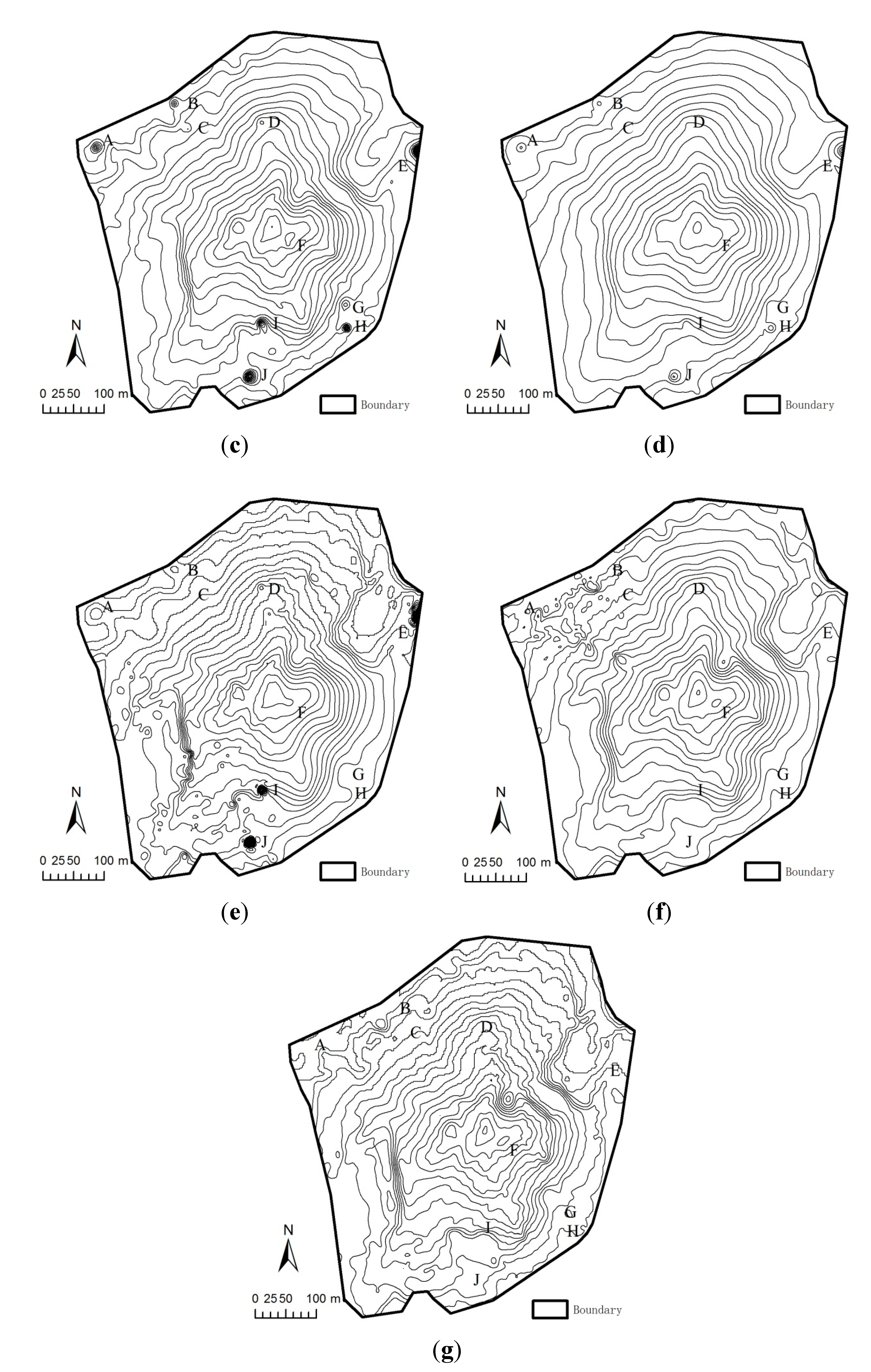
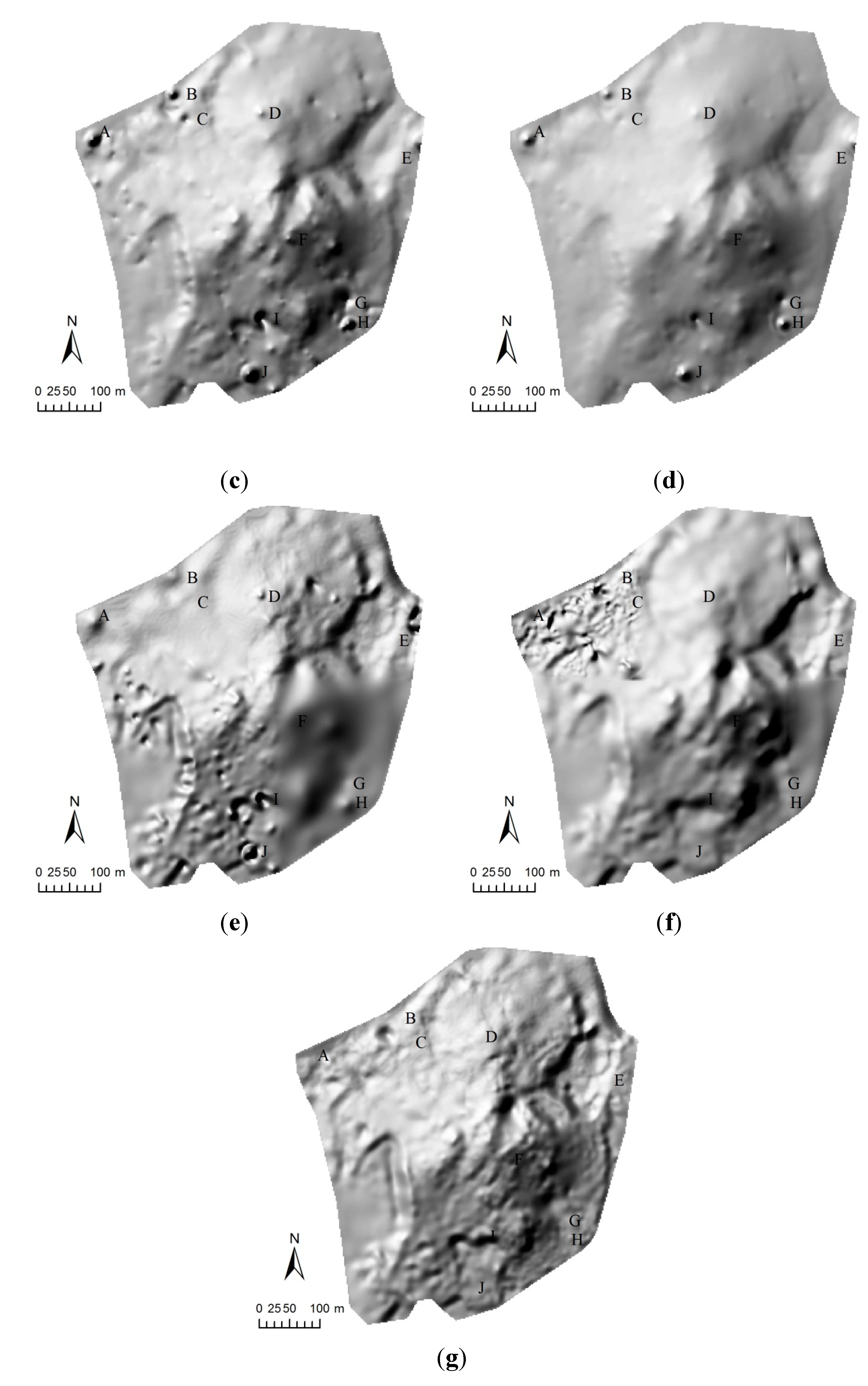
4.2. A Real-World Example

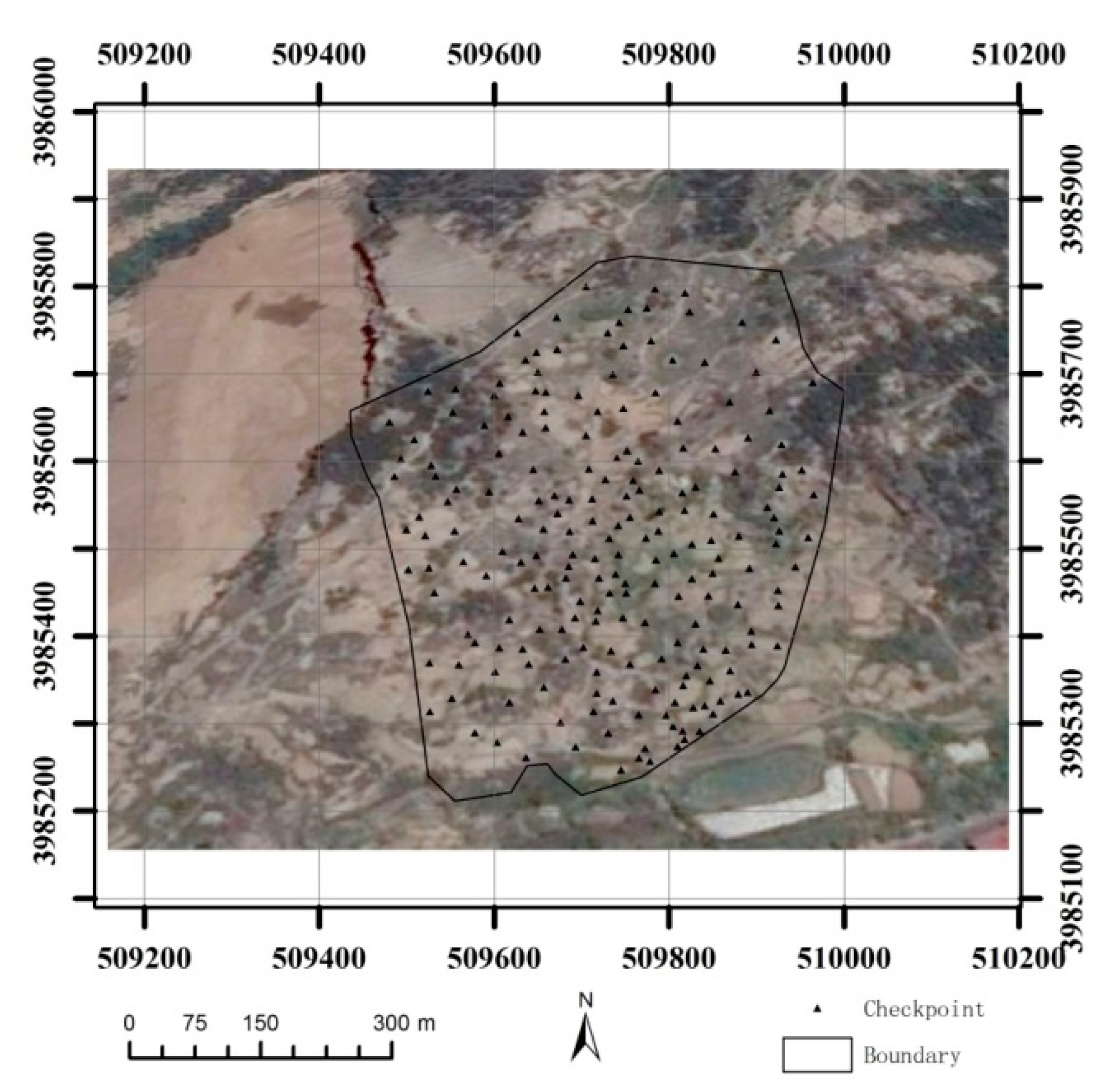
4.2.1. Study Site and Data Capture

The study site with an area of about 0.46 km² is located in Shandong province, China. The terrain is mainly characterized as non-karstic with some isolated trees (Figure 3). The Gauss–Krueger projection, in which each zone is 3° of longitude in width, was adopted to transform the National Geodetic Coordinate System 1980 into rectangular Cartesian coordinates. The elevation datum was National Height Datum 1985. The elevations of this study site range from 28 m to 231 m with the mean of 78.3 m and the standard deviation of 22.6 m. The survey was carried out on 12 November 2012. Two Canon EOS 5D-Mark II cameras were mounted on the UAV for taking photos. The mean flying height of the UAV above the ground (relative flying height) was about 350 m. The photographic scale was 1:12,000 with an image of 5616 × 3744 pixels and the ground resolution of 8 cm. The side overlapping proportion of two neighbor images was about 50%, and the forward overlapping proportion was 80%. All images were processed with an automatic air triangulation (AT) mapping software termed Map-AT, developed by Chinese Academy of Survey & Mapping. After the stereo-image processing, about 6797 points were extracted. Namely, the average point space (PS) is about 0.15 m. In total, 203 checkpoints (Figure 3) randomly sampled using RTK GNSS with vertical root mean square error (RMSE) of 2 cm and horizontal RMSE of 1 cm were used to test the interpolation accuracy. The checkpoints were selected by three surveyors under the rule of data accuracy and personal safety. Namely, the signal of RTK GNSS must be strong, and some places that are difficult to reach are not sampled.

Figure 3. Digital orthophoto map of the study site in the real-world example (The Gauss–Krueger projection was adopted to transform the National Geodetic Coordinate System 1980 into rectangular Cartesian coordinates. The elevation datum was National Height Datum 1985.)

Figure 3. Digital orthophoto map of the study site in the real-world example (The Gauss–Krueger projection was adopted to transform the National Geodetic Coordinate System 1980 into rectangular Cartesian coordinates. The elevation datum was National Height Datum 1985.)

4.2.2. Interpolation Methods

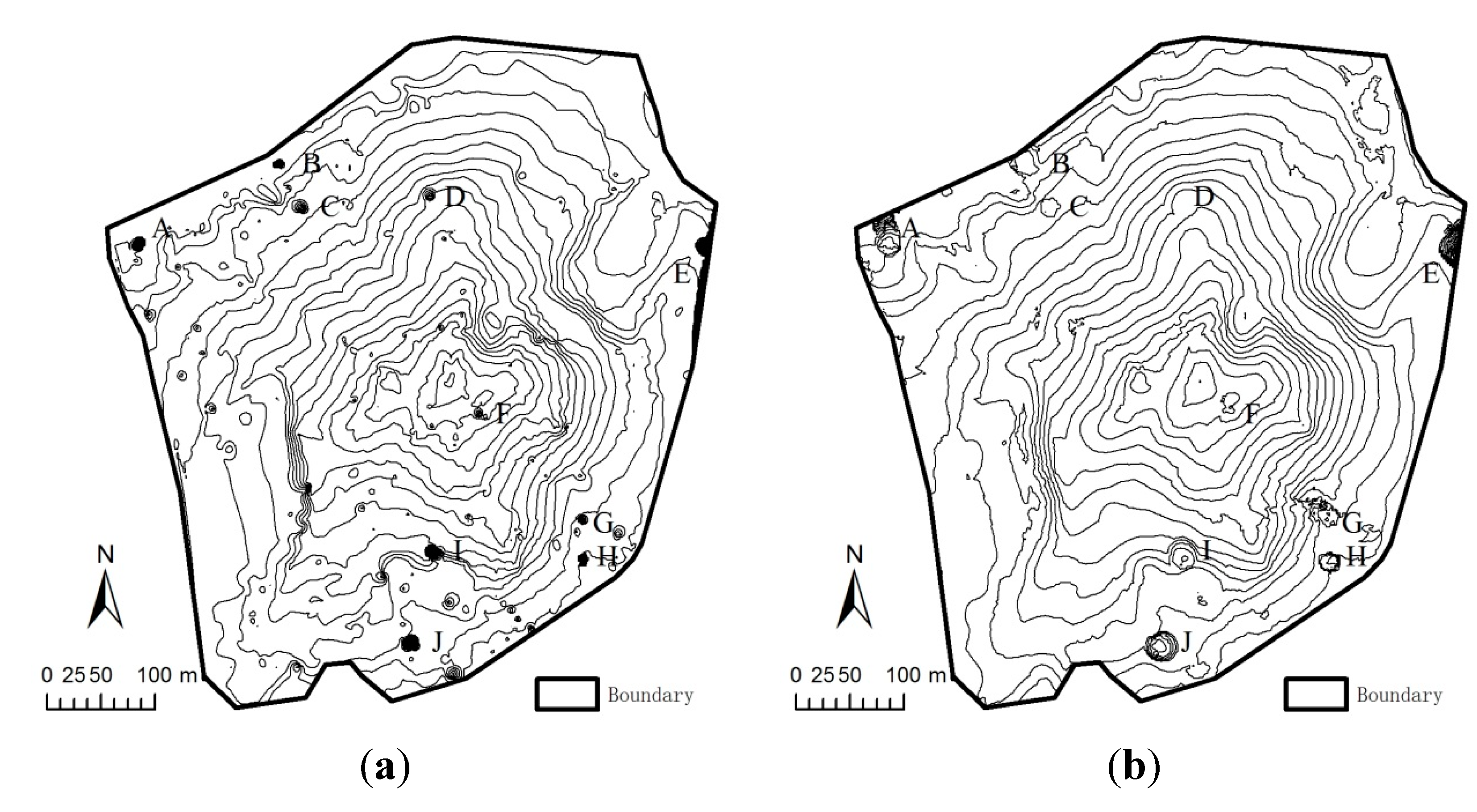
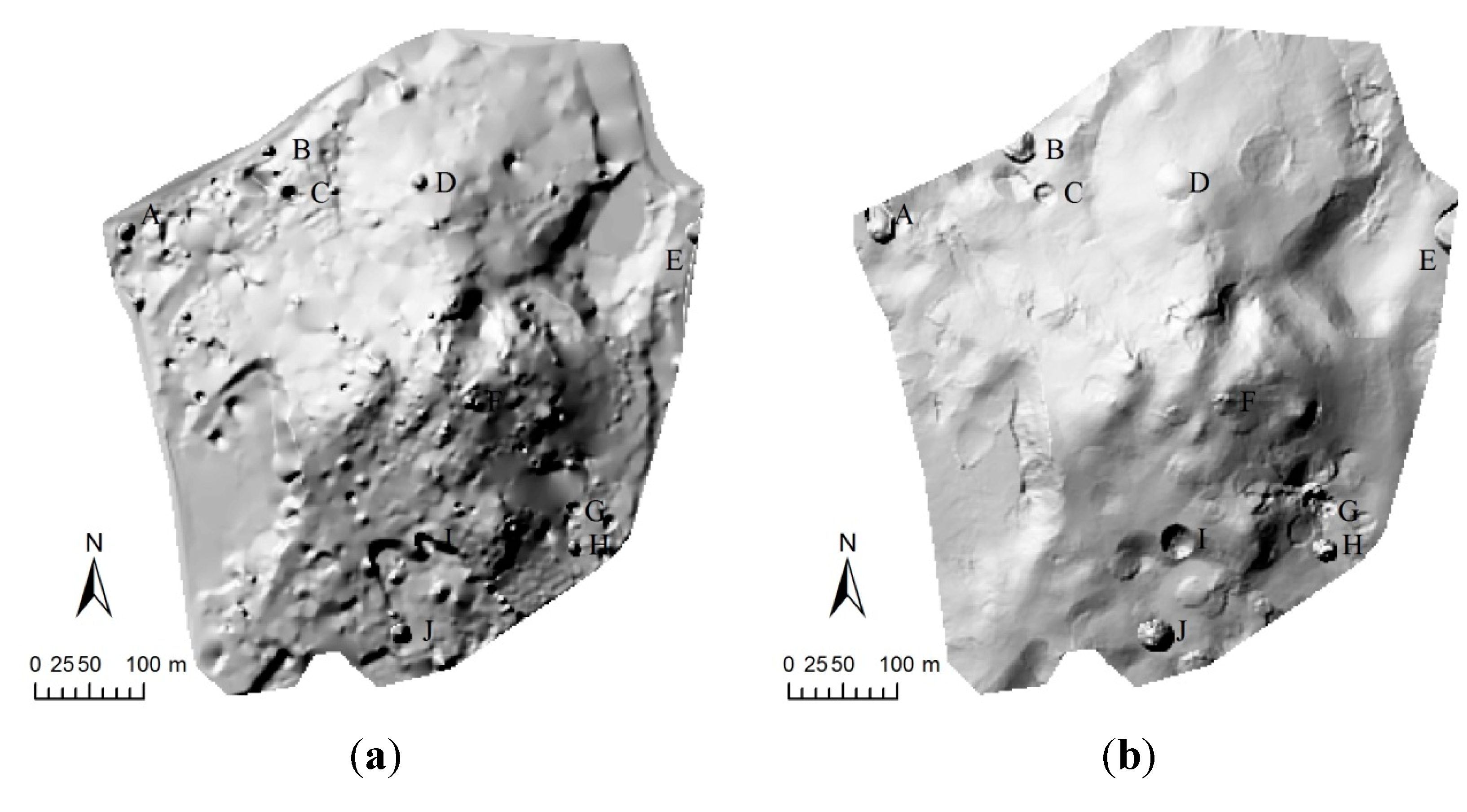
In addition to the three versions of MQ, including MQ-IH, MQ-CH and the classical MQ, the classical interpolation methods, including NN, OK and ANUDEM, were also employed to construct DEMs. In principle, the three classical interpolation methods have their respective features. NN and OK are, respectively, representative of exact and smoothing interpolators, which are widely adopted for remote-sensing-derived DEM construction [18,20,52,53]. NN is based on Voronoi tessellation of a discrete set of spatial points. It is very simple to perform, as no parameter should be assigned. The performance of OK is seriously determined by the semivariogram, which must be manually fitted before performing interpolations. ANUDEM is an interpolation method specifically designed for the creation of hydrologically correct digital elevation models (DEMs) [54,55]. The robustness of ANUDEM is determined by the parameter “vertical standard error”. In our paper, OK was performed in the GS+ geostatistics software [56]. GS+ provides all geostatistics components, from semivariance analysis through kriging and mapping, in a single integrated software program widely praised for its flexibility and friendly interface. ANUDEM was performed in the “Spatial Analyst Tools” module of ArcGIS 10.1 with the “topo to raster” command, where the optimal value of the parameter “vertical standard error” was determined by trial and error. NN was also performed with ArcGIS 10.1.

In the first group of tests, the aforementioned interpolation methods were, respectively, employed to construct 2 m DEMs with all sample points. In order to conduct a qualitative comparison, the shaded relief maps and contour lines with 5 m interval of all interpolation methods were formed. In the second group, we tested the effect of sample density on the accuracy of interpolation methods by collecting two groups of points with different sample densities from the raw points, and the interpolation results were measured by the 203 checkpoints.

4.2.3. Results

NN is an exact interpolator, which can show the raw nature of sample points. It can be seen from Figure 4a that there are a considerable number of densely closed contours representing artificial depressions and erratic mounds at the locations A–J. This indicates that many erroneous values exist in the raw sample points. Labeling these points on the satellite image of this study site, we found that they are mainly located either at the low contrast and featureless regions, or at steep slope regions of rugged hills, where the automatic image matching algorithm always fails. In addition, some points are located on trees, which can be considered as outliers in the context of DEM construction. In conclusion, the raw elevation points suffer from noise and outliers.

Figure 4. Contours of (a) NN; (b) OK; (c) ANUDEM with 5 m vertical standard deviation error (ANUDEM5); (d) ANUDEM with 6 m vertical standard deviation error (ANUDEM6); (e) classical MQ; (f) MQ-CH; and (g) MQ-IH.

Figure 4. Contours of (a) NN; (b) OK; (c) ANUDEM with 5 m vertical standard deviation error (ANUDEM5); (d) ANUDEM with 6 m vertical standard deviation error (ANUDEM6); (e) classical MQ; (f) MQ-CH; and (g) MQ-IH.

For OK (Figure 4b), the densely closed contours at the locations B–D and F disappear. For ANUDEM with 5 m vertical standard deviation error (ANUDEM5) (Figure 4c), the densely closed contours at the locations C, D, F and J disappear. For ANUDEM with 6 m vertical standard deviation error (ANUDEM6) (Figure 4d), almost all of the densely closed contours disappear, except for the locations E and J. In addition, the small closed contours sporadically distributed in Figure 4a disappear in the maps of OK and ANUDEM. This indicates that OK and ANUDEM are less influenced by outliers than NN. The above results can be expected, as both OK and ANUDEM are smoothing interpolation methods, which can smooth noise inherent in sample points. For MQ (Figure 4e), the densely closed contours at the locations A–D and F–H disappear. For MQ-CH (Figure 4f), all densely closed contours disappear. However, some small closed contours are sporadically distributed in the upper-left. In comparison, MQ-IH is more robust to outliers than the other methods, which is demonstrated by the fact that all the densely closed contours at the locations A–J completely disappear, and are replaced by smooth contour lines with a natural appearance (Figure 4g).

The shaded relief map of NN is fragmented with many isolated pits and mounds (Figure 5a). This indicates that NN is very sensitive to outliers. The map of OK is smoother than that of NN. However, some erratic pits and artificial mounds still exist, especially at the locations A–J (Figure 5b). With the adjustment of vertical standard deviation error, ANUDEM seems to have the ability to resist outliers (Figure 4c,d). However, observing the maps of ANUDEM5 and ANUDEM6, we can find that ANUDEM possesses the robustness at the cost of losing subtle terrain features (Figure 5c,d). MQ is also influenced by the outliers, proved by the isolated pits and mounds at the locations A and D–J (Figure 5e). The effect of outliers is obviously decreased by MQ-CH (Figure 5f). However, MQ-CH has a coarse surface at the upper-left, and at other locations, its surface is so smooth that many subtle terrain features are lost. Comparatively, MQ-IH has a better ability of decreasing the effect of outliers, while retaining the subtle terrain features (Figure 5g). For example, the erosion cliff in the left bottom is kept very well. The erroneous pits and mounds at the locations A–J disappear and the surface keeps good continuity at these locations. Hence, we can conclude that MQ-IH is more robust to outliers than the classical interpolation methods for interpolating remote-sensing-derived elevation data set.

Figure 5. Shaded relief maps of (a) NN; (b) OK; (c) ANUDEM with 5 m vertical standard deviation error (ANUDEM5); (d) ANUDEM with 6 m vertical standard deviation error (ANUDEM6), (e) classical MQ; (f) MQ-CH and (g) MQ-IH.

Figure 5. Shaded relief maps of (a) NN; (b) OK; (c) ANUDEM with 5 m vertical standard deviation error (ANUDEM5); (d) ANUDEM with 6 m vertical standard deviation error (ANUDEM6), (e) classical MQ; (f) MQ-CH and (g) MQ-IH.

Based on the checkpoints, we tested the effect of sample density on the interpolation accuracy of MQ-IH. Namely, three groups of data sets with different point spaces (PSs) were, respectively, collected from the original sampling points to construct 2 m DEMs. The PSs obtained were those shown in Table 2, i.e., from 0.15 m to 0.3 m.

Table 2. Relationship between the number of sample points and average point space.

Number of Sample Points	6797	3822	1699
Point space (m)	0.15	0.2	0.3

Table 2. Relationship between the number of sample points and average point space.

Number of Sample Points	6797	3822	1699
Point space (m)	0.15	0.2	0.3

Simulation results (Table 3) demonstrate that regardless of interpolation methods, the estimation accuracy decreases with the increasing PS. Irrespective of accuracy measures, MQ-IH is always more accurate than other interpolation methods in terms of RMSE and MinE. However, the MaxE of MQ-IH is slightly bigger than those of NN, OK, ANUDEM5 and ANUDEM6, which may be caused by the fact that some feature points at rough terrain are overly smoothed by MQ.

Table 3. Accuracy comparison between different interpolation methods in the real-world example (unit: m).

PS	Accuracy Measures	Methods
		NN	OK	ANUDEM5	ANUDEM6	MQ	MQ-CH	MQ-IH
0.15	RMSE	1.91	1.38	2.38	2.36	2.80	1.17	0.97
	MaxE	1.36	1.60	2.02	1.66	5.02	4.36	3.80
	MinE	−25.74	−18.00	−33.14	−32.76	−35.17	−5.58	−5.55
0.2	RMSE	2.35	1.58	2.59	2.47	2.94	1.24	1.05
	MaxE	1.98	1.95	2.32	1.88	5.42	4.57	4.02
	MinE	−25.88	−18.72	−33.97	−33.14	−35.84	−5.94	−5.91
0.3	RMSE	2.89	1.91	2.87	2.72	3.11	1.45	1.22
	MaxE	2.04	2.03	2.68	2.03	5.88	5.01	4.88
	MinE	−30.12	−19.11	−34.45	−34.00	−36.17	−6.06	−6.03

Table 3. Accuracy comparison between different interpolation methods in the real-world example (unit: m).

PS	Accuracy Measures	Methods
		NN	OK	ANUDEM5	ANUDEM6	MQ	MQ-CH	MQ-IH
0.15	RMSE	1.91	1.38	2.38	2.36	2.80	1.17	0.97
	MaxE	1.36	1.60	2.02	1.66	5.02	4.36	3.80
	MinE	−25.74	−18.00	−33.14	−32.76	−35.17	−5.58	−5.55
0.2	RMSE	2.35	1.58	2.59	2.47	2.94	1.24	1.05
	MaxE	1.98	1.95	2.32	1.88	5.42	4.57	4.02
	MinE	−25.88	−18.72	−33.97	−33.14	−35.84	−5.94	−5.91
0.3	RMSE	2.89	1.91	2.87	2.72	3.11	1.45	1.22
	MaxE	2.04	2.03	2.68	2.03	5.88	5.01	4.88
	MinE	−30.12	−19.11	−34.45	−34.00	−36.17	−6.06	−6.03

In order to test the computational cost of the aforementioned interpolation methods, their computing time for interpolating 2 m DEM with 6797 points was shown in Table 4. It should be noted that the computing time of OK is difficult to count due to the manual operation for fitting the semivarogram. Thus, its time is not list. Results (Table 4) indicate that NN is the fastest method. This result can be expected, as NN need not solve any system of linear equations. The two versions of ANUDEM are much faster than the three versions of MQ. This is due to the fact that ANUDEM is based on a finite difference technique to perform surface modeling, and one solution of the system of linear equations can achieve the simulation results. Furthermore, the system of ANUDEM is very sparse, so it can be efficiently solved [57]. However, MQ is a point-to-point interpolator. Namely, we must solve one system of linear equations to compute the value of one point, which brings huge computational cost for modeling the whole surface. Results also show that the classical MQ has a higher speed than MQ-CH and MQ-IH. This is because the latter two employ an iterative process to decrease the effect of outliers on surface modeling.

In a word, the real-world example indicates that MQ-IH is more accurate than the classical interpolation methods for DEM construction in terms of both quantitative and qualitative analysis. However, its computational cost is much bigger than that of the classical interpolation methods.

Table 4. Computing time of all interpolation methods for interpolating 2 m DEM with 6797 sample points.

Methods	Time (s)
NN	6.28
OK	-
ANUDEM5	20.34
ANUDEM6	20.34
Classical MQ	63.25
MQ-CH	150.17
MQ-IH	150.17

Table 4. Computing time of all interpolation methods for interpolating 2 m DEM with 6797 sample points.

Methods	Time (s)
NN	6.28
OK	-
ANUDEM5	20.34
ANUDEM6	20.34
Classical MQ	63.25
MQ-CH	150.17
MQ-IH	150.17

5. Discussion

Recently, Chen and Li [58] presented a least absolute deviation (LAD)-based MQ (MQ-L) for decreasing the impact of outliers on DEM construction. Namely, MQ-L takes the least sum of absolute deviation as the objective function. It includes two independent procedures, i.e., the selection of some significant knots with a space-filling design and the solution of a linear system with LAD. Results indicated that MQ-L is more accurate than the classical MQ when sample points are subject to outliers. However, there are three major shortcomings of MQ-L: (1) LAD does not completely avoid the impact of outliers due to the least absolute deviation loss function; (2) the optimal number of knots is difficult to determine (in practice, it is subjectively set as the tenth of the total number of sample points); and (3) LAD has a huge memory cost, which seriously restricts its widespread applications in practice. In order to compare the performance of MQ-IH with that of MQ-L, the data sets in the numerical test of this paper were simulated by MQ-L. Results (Table 1) show that MQ-L is more robust to outliers than the classical MQ when sample points are subject to outliers (i.e., Cases 2 and 3). This conclusion is consistent with that obtained in the paper of Chen and Li [58]. However, MQ-IH is always more accurate than MQ-L, regardless of error distributions. This further validates the high robustness of MQ-IH.

It should be noted that spatial outliers in a statistical sense are not definitely erroneous data although they are highly likely to be so [31]. Instead of being simply removed, spatial outliers should be further checked with some prior knowledge to determine whether they should be retained or eliminated. For example, in the real-world example of this paper, we can superimpose outliers (i.e., observations with residuals belonging to A₀ or A₄ in the improved Huber loss function) on satellite images for error verification. The outliers located at a smooth terrain are definitely erroneous data. However, if outliers were located at natural cliffs, steep gorges, mounds or pits, they certainly contain important terrain features and hence should be retained. So, in the context of surface modeling with MQ-IH, the residuals of these retained outliers should belong to A₂ in the improved Huber loss function.

Like the classical interpolation methods, elevation sample points and contour lines captured by any instruments or techniques can be used as the input data when performing interpolations with MQ-IH. However, compared with the classical interpolation methods, MQ-IH is more effective to remote-sensing-derived elevation data sets, since they often suffer from noise and outliers due to various reasons, such as the physical limitations of sensors, multiple reflectance, occlusions and low contrast of texture.

6. Conclusions

In this paper, we have developed a robust method of multiquadric method (MQ) based on an Improved Huber loss function (MQ-IH) for carrying out interpolations when spatial points are subject to outliers. The numerical test with the simulated model errors show that MQ-IH is more robust than MQ based on the classical Huber loss function (MQ-CH) and the classical MQ for surface modeling when sample points suffer from outliers, and MQ-IH has high efficiency when sample points follow a normal distribution. For example, for the Cauchy error distribution with the location parameter of 0 and scale parameter of 1, the RMSEs of MQ-CH and the classical MQ are 0.3916 and 1.4591, respectively, whereas that of MQ-IH is 0.3698. The real-world example of DEM construction with stereo-images-derived elevation data set demonstrates that MQ-IH outperforms the classical interpolation methods including NN, OK and ANUDEM, and the two versions of MQ including the classical MQ and MQ-CH. Specifically, NN is seriously influenced by outliers, which leads to the densely closed contour lines with an unnatural appearance and the fragmented shaded relief map with many artificial pits and erroneous mounds. OK is slightly better than NN. Nevertheless, some unnatural contours still exist and its map is so smooth than many terrain features like erosion cliffs are lost. ANUDEM is capable of resisting the effect of outliers with an adjustment of vertical standard deviation, but this is at the cost of losing some subtle terrain features. The classical MQ suffers from densely closed contour lines, artificial pits and erroneous mounds in the shaded relief map. MQ-CH is slightly better than MQ, but its surface is so smooth that many subtle terrain features are lost. Comparatively, MQ-IH has a better ability of maximally decreasing the effect of outliers, while faithfully keeping terrain features. When interpolating the 2 m DEM with the 6797 sample points in terms of quantitative analysis, the RMSEs of NN, OK, ANUDEM with 5 m and 6 m vertical standard deviation errors, the classical MQ and MQ-CH are 1.91 m, 1.38 m, 2.38 m, 2.36 m, 2.80 m and 1.17 m, respectively, whereas that of MQ-IH is only 0.97 m. Yet, MQ-IH has much bigger computing cost than the classical interpolation methods. In addition, MQ-IH has coarser contours than ANUDEM in the upper location of the real-world study site, and its shaded relief map may not satisfactorily conform to the real-world surface at rough terrain.

Theoretically, the well performance of MQ-IH can be attributed to the high interpolation accuracy of MQ for surface modeling and the high robustness of the improved Huber loss function to outliers. Based on MQ, surfaces with complex terrain morphologies can be accurately simulated. With the improved Huber loss function, the contribution of a point to MQ-based surface modeling is significantly determined by its sample error. Theoretically, when the error of a sample point is more than three times as big as the standard deviation of all sample errors, the point is considered as an outlier and then have no effect on surface modeling. Thus, MQ-IH has high robustness to outliers. In conclusion, MQ-IH has great potential for interpolating remote-sensing-derived elevation data sets.

In principle, a data set can contain four types of points including regular observations, vertical outliers, good leverage points and bad leverage points [8]. It should be noted that the bad leverage points also belong to outliers. In this paper, MQ-IH can only resist the effect of vertical outliers, as the improved Huber loss function is not robust to the bad leverage points. At present, the least sum of trimmed squares (LTS) has been widely accepted as a robust objective function for resisting vertical outliers and bad leverage points because of its highly statistical efficiency and high breakdown point [59]. Hence, our further work is to improve the robustness of MQ by using the LTS as the loss function for remote-sensing-derived DEM construction in study sites with different terrain morphologies, such as flat, rolling, karstic and mountainous areas.

References

1. Wilson, J.P. Digital terrain modeling. Geomorphology 2012, 137, 107–121. [Google Scholar] [CrossRef]
2. Baltsavias, E.P. A comparison between photogrammetry and laser scanning. ISPRS J. Photogramm. Remote Sens. 1999, 54, 83–94. [Google Scholar] [CrossRef]
3. Gamba, P.; DELL’ACQUA, F.; Houshmand, B. Comparison and fusion of LiDAR and InSAR digital elevation models over urban areas. Int. J. Remote Sens. 2003, 24, 4289–4300. [Google Scholar] [CrossRef]
4. Liu, H.; Jezek, K.C.; O’Kelly, M.E. Detecting outliers in irregularly distributed spatial data sets by locally adaptive and robust statistical analysis and GIS. Int. J. Geogr. Inf. Sci. 2001, 15, 721–741. [Google Scholar] [CrossRef]
5. Sun, X.; Rosin, P.L.; Martin, R.R.; Langbein, F.C. Noise in 3D laser range scanner data. In Proceedings of the IEEE International Conference on Shape Modeling and Applications, Stony Brook, NY, USA, 4–6 June 2008; pp. 37–45.
6. Nurunnabi, A.; Belton, D.; West, G. Robust statistical approaches for local planar surface fitting in 3D laser scanning data. ISPRS J. Photogramm. Remote Sens. 2014, 96, 106–122. [Google Scholar] [CrossRef]
7. Höhle, J.; Höhle, M. Accuracy assessment of digital elevation models by means of robust statistical methods. ISPRS J. Photogramm. Remote Sens. 2009, 64, 398–406. [Google Scholar] [CrossRef]
8. Rousseeuw, P.J.; Hubert, M. Robust statistics for outlier detection. Wiley Interdiscip. Rev. Data Min. Knowl. Discov. 2011, 1, 73–79. [Google Scholar] [CrossRef]
9. Barnett, V.; Lewis, T. Outliers in Statistical Data; Wiley: New York, NY, USA, 1994; Volume 3. [Google Scholar]
10. Höhle, J. Assessing the positional accuracy of airborne laser scanning in urban areas. Photogramm. Record 2013, 28, 196–210. [Google Scholar] [CrossRef]
11. Aguilar, F.J.; Mills, J.P. Accuracy assessment of lidar-derived digital elevation models. Photogramm. Record 2008, 23, 148–169. [Google Scholar] [CrossRef]
12. Soudarissanane, S.; Lindenbergh, R.; Menenti, M.; Teunissen, P. Scanning geometry: Influencing factor on the quality of terrestrial laser scanning points. ISPRS J. Photogramm. Remote Sens. 2011, 66, 389–399. [Google Scholar] [CrossRef]
13. Sun, X.; Rosin, P.L.; Martin, R.R.; Langbein, F.C. Noise analysis and synthesis for 3D laser depth scanners. Graph. Models 2009, 71, 34–48. [Google Scholar] [CrossRef]
14. Rousseeuw, P.; Leroy, A. Robust Regression and Outlier Detection; Wiley-IEEE: New York, NY, USA, 2003. [Google Scholar]
15. Chen, C.F.; Yue, T.X.; Dai, H.L.; Tian, M.Y. The smoothness of HASM. Int. J. Geogr. Inf. Sci. 2013, 27, 1651–1667. [Google Scholar] [CrossRef]
16. Alfons, A.; Croux, C.; Gelper, S. Sparse least trimmed squares regression for analyzing high-dimensional large data sets. Ann. Appl. Stat. 2013, 7, 226–248. [Google Scholar] [CrossRef]
17. Chen, C.F.; Fan, Z.M.; Yue, T.X.; Dai, H.L. A robust estimator for the accuracy assessment of remote-sensing-derived DEMs. Int. J. Remote Sens. 2012, 33, 2482–2497. [Google Scholar] [CrossRef]
18. Bater, C.W.; Coops, N.C. Evaluating error associated with lidar-derived DEM interpolation. Comput. Geosci. 2009, 35, 289–300. [Google Scholar] [CrossRef]
19. Lloyd, C.; Atkinson, P. Deriving DSMs from LiDAR data with kriging. Int. J. Remote Sens. 2002, 23, 2519–2524. [Google Scholar] [CrossRef]
20. Lloyd, C.D.; Atkinson, P.M. Deriving ground surface digital elevation models from LiDAR data with geostatics. Int. J. Geogr. Inf. Sci. 2006, 20, 535–563. [Google Scholar] [CrossRef]
21. Franke, R. Scattered data interpolation: Tests of some method. Math. Comput. 1982, 38, 181–200. [Google Scholar]
22. Aguilar, F.J.; Aguera, F.; Aguilar, M.A.; Carvajal, F. Effects of terrain morphology, sampling density, and interpolation methods on grid DEM accuracy. Photogramm. Eng. Remote Sens. 2005, 71, 805–816. [Google Scholar] [CrossRef]
23. Huber, P.J. Robust Statistics; Wiley-Interscience: New York, NY, USA, 2004. [Google Scholar]
24. Ester, M.; Kriegel, H.P.; Sander, J.; Xu, X. A Density-Based Algorithm for Discovering Clusters in Large Spatial Databases with Noise. Available online: http://www.dbs.ifi.lmu.de/Publikationen/Papers/KDD-96.final.frame.pdf (accessed on 12 January 2015).
25. Su, X.; Tsai, C.L. Outlier detection. Wiley Interdiscip. Rev. Data Min. Knowl. Discov. 2011, 1, 261–268. [Google Scholar] [CrossRef]
26. Ruts, I.; Rousseeuw, P.J. Computing depth contours of bivariate point clouds. Comput. Stat. Data Anal. 1996, 23, 153–168. [Google Scholar] [CrossRef]
27. Lu, C.T.; Santos, R.F.D.O.S.; Liu, X.; Kou, Y. A graph-based approach to detect abnormal spatial points and regions. Int. J. Artif. Intell. Tools 2011, 20, 721–751. [Google Scholar] [CrossRef]
28. Breunig, M.M.; Kriegel, H.P.; Ng, R.T.; Sander, J. LOF: Identifying density-based local outliers. ACM SIGMOD Record 2000, 29, 93–104. [Google Scholar] [CrossRef]
29. Knorr, E.M.; Ng, R.T.; Tucakov, V. Distance-based outliers: Algorithms and applications. VLDB J. 2000, 8, 237–253. [Google Scholar] [CrossRef]
30. Chawla, S.; Sun, P. SLOM: A new measure for local spatial outliers. Knowl. Inf. Syst. 2006, 9, 412–429. [Google Scholar] [CrossRef]
31. Chen, D.; Lu, C.T.; Kou, Y.; Chen, F. On detecting spatial outliers. GeoInformatica 2008, 12, 455–475. [Google Scholar] [CrossRef]
32. MacEachren, A.M.; Robinson, A.; Hopper, S.; Gardner, S.; Murray, R.; Gahegan, M.; Hetzler, E. Visualizing geospatial information uncertainty: What we know and what we need to know. Cartogr. Geogr. Inf. Sci. 2005, 32, 139–160. [Google Scholar] [CrossRef]
33. Podobnikar, T. Methods for visual quality assessment of a digital terrain model. SAPI. EN. S. Surv. Perspect. Integr. Environ. Soc. 2009, 2, 15–24. [Google Scholar]
34. Haining, R. Spatial Data Analysis in the Social and Environmental Sciences; Cambridge University Press: Cambridge, UK, 1993. [Google Scholar]
35. Anselin, L. The Moran scatterplot as an ESDA tool to assess local instability in spatial association. Spat. Anal. Perspect. GIS 1996, 111, 111–125. [Google Scholar]
36. Giménez, E.; Crespi, M.; Garrido, M.S.; Gil, A.J. Multivariate outlier detection based on robust computation of Mahalanobis distances. Application to positioning assisted by RTK GNSS Networks. Int. J. Appl. Earth Obs. Geoinf. 2012, 16, 94–100. [Google Scholar] [CrossRef]
37. Nurunnabi, A.; West, G.; Belton, D. Outlier detection and robust normal-curvature estimation in mobile laser scanning 3D point cloud data. Pattern Recog. 2015, 48, 1400–1415. [Google Scholar]
38. Fleishman, S.; Cohen-Or, D.; Silva, C.T. Robust moving least-squares fitting with sharp features. ACM Trans. Graph. 2005, 24, 544–552. [Google Scholar] [CrossRef]
39. Fischler, M.A.; Bolles, R.C. Random sample consensus: A paradigm for model fitting with applications to image analysis and automated cartography. Commun. ACM 1981, 24, 381–395. [Google Scholar] [CrossRef]
40. Schnabel, R.; Wahl, R.; Klein, R. Efficient RANSAC for point-cloud shape detection. Comput. Graph. Forum 2007, 26, 214–226. [Google Scholar] [CrossRef]
41. Masuda, H.; Tanaka, I.; Enomoto, M. Reliable surface extraction from point-clouds using scanner-dependent parameters. Comput. Aid. Design Appl. 2013, 10, 265–277. [Google Scholar] [CrossRef]
42. Torr, P.H.S.; Zisserman, A. MLESAC: A new robust estimator with application to estimating image geometry. Comput. Vision Image Underst. 2000, 78, 138–156. [Google Scholar] [CrossRef]
43. Debese, N.; Moitié, R.; Seube, N. Multibeam echosounder data cleaning through a hierarchic adaptive and robust local surfacing. Comput. Geosci. 2012, 46, 330–339. [Google Scholar] [CrossRef]
44. Rousseeuw, P.J.; Driessen, K.V. A fast algorithm for the minimum covariance determinant estimator. Technometrics 1999, 41, 212–223. [Google Scholar] [CrossRef]
45. Hubert, M.; Rousseeuw, P.J.; Vanden Branden, K. ROBPCA: A new approach to robust principal component analysis. Technometrics 2005, 47, 64–79. [Google Scholar] [CrossRef]
46. Garcia, D. Robust smoothing of gridded data in one and higher dimensions with missing values. Comput. Stat. Data Anal. 2010, 54, 1167–1178. [Google Scholar] [CrossRef] [PubMed]
47. Hardy, R. Theory and applications of the multiquadric-biharmonic method 20 years of discovery 1968–1988. Comput. Math. Appl. 1990, 19, 163–208. [Google Scholar] [CrossRef]
48. Rippa, S. An algorithm for selecting a good value for the parameter c in radial basis function interpolation. Adv. Comput. Math. 1999, 11, 193–210. [Google Scholar] [CrossRef]
49. Chen, C.F.; Yan, C.Q.; Cao, X.W.; Guo, J.Y.; Dai, H.L. A greedy-based multiquadric method for LiDAR-derived ground data reduction. ISPRS J. Photogramm. Remote Sens. 2015, 102, 110–121. [Google Scholar] [CrossRef]
50. Rousseeuw, P.J.; Croux, C. Alternatives to the median absolute deviation. J. Am. Stat. Assoc. 1993, 88, 1273–1283. [Google Scholar] [CrossRef]
51. An, S.; Liu, W.; Venkatesh, S. Fast cross-validation algorithms for least squares support vector machine and kernel ridge regression. Pattern Recog. 2007, 40, 2154–2162. [Google Scholar] [CrossRef]
52. Bailly, J.S.; Le Coarer, Y.; Languille, P.; Stigermark, C.J.; Allouis, T. Geostatistical estimations of bathymetric LiDAR errors on rivers. Earth Surf. Process. Landf. 2010, 35, 1199–1210. [Google Scholar] [CrossRef]
53. Grohmann, C.H.; Steiner, S.S. SRTM resample with short distance-low nugget kriging. Int. J. Geogr. Inf. Sci. 2008, 22, 895–906. [Google Scholar] [CrossRef]
54. Hutchinson, M.F. A new procedure for gridding elevation and stream line data with automatic removal of spurious pits. J. Hydrol. 1989, 106, 211–232. [Google Scholar] [CrossRef]
55. Hutchinson, M.F.; Xu, T.; Stein, J.A. Recent Progress in the ANUDEM Elevation Gridding Procedure. Available online: http://geomorphometry.org/system/files/HutchinsonXu2011geomorphometry.pdf (accessed on 12 January 2015).
56. Robertson, G.P. Geostatistics for Environmental Sciences, GS+ Users Guide, Version 5; Gamma Design Software: Plainwell, MI, USA, 2008. [Google Scholar]
57. Hutchinson, M.F. A locally adaptive approach to the interpolation of digital elevation models. In Proceedings of the Third International Conference/Workshop on Integrating GIS and Environmental Modeling NCGIA, University of California, Oakland, CA, USA, 21–25 January 1996; pp. 21–26.
58. Chen, C.F.; Li, Y.Y. A robust multiquadric method for digital elevation model construction. Math. Geosci. 2013, 45, 297–319. [Google Scholar] [CrossRef]
59. Rousseeuw, P.J.; van Driessen, K. Computing LTS regression for large data sets. Data Min. Knowl. Discov. 2006, 12, 29–45. [Google Scholar] [CrossRef]