Monitoring of Irrigation Schemes by Remote Sensing: Phenology versus Retrieval of Biophysical Variables

Abstract
:
1. Introduction
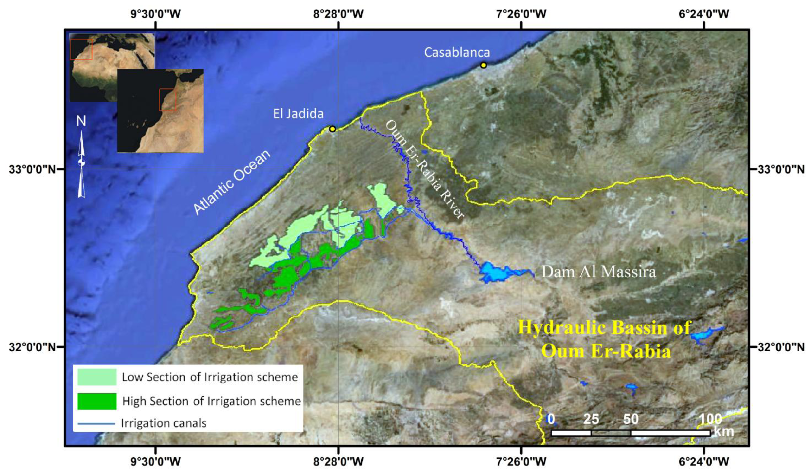
2. Study Area
3. Data Collection
3.1. Satellite Data
3.2. Meteorological and Water Flow Data
3.3. Data In-Situ
4. Methods
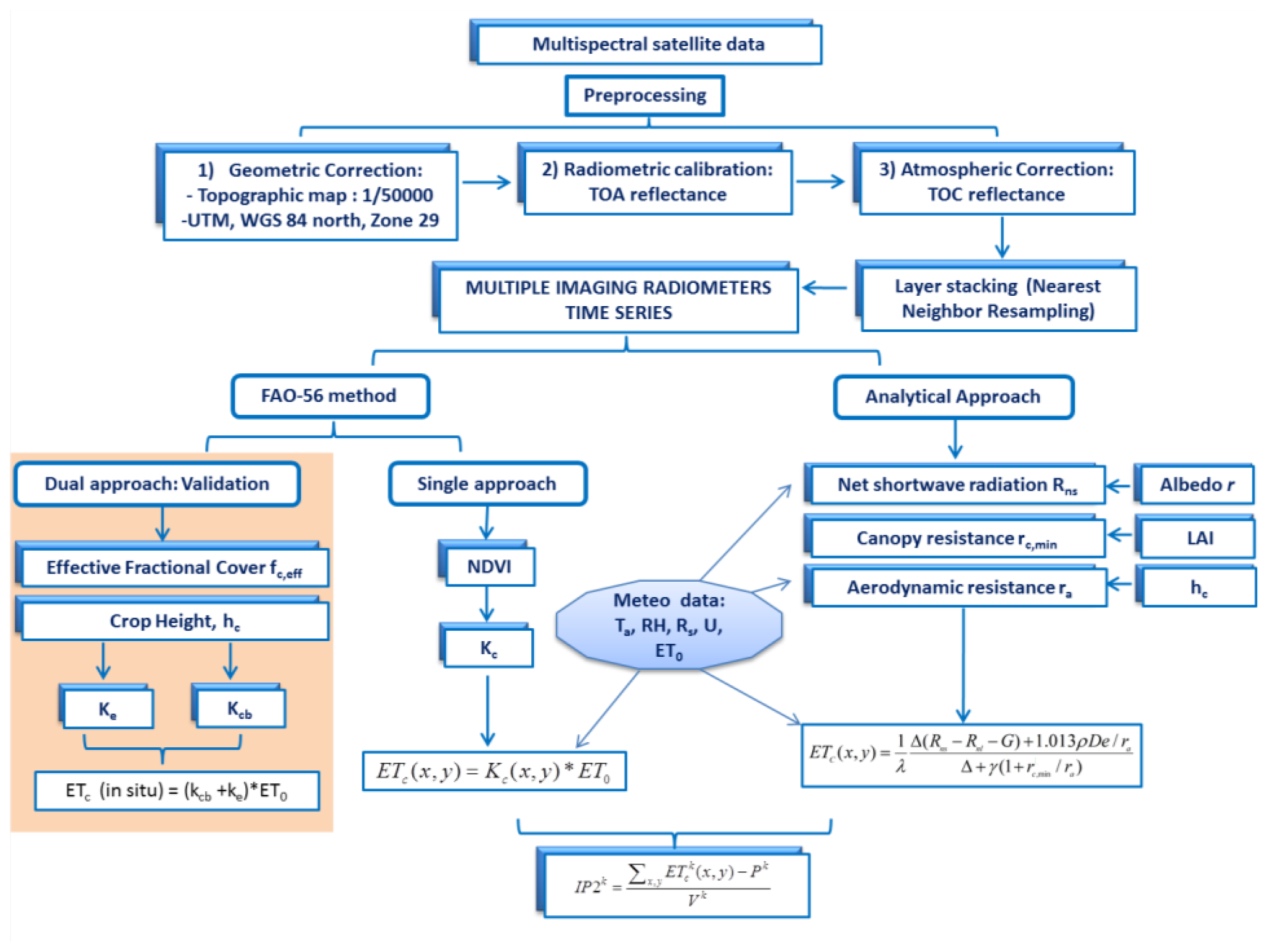
4.1. Work Flow
4.2. Pre-Processing
4.3. Application of FAO-56 Model
4.3.1. Single Crop Coefficient Approach: kc-NDVI Method
4.3.2. Dual Crop Coefficient Approach
- Kcb-mid is the estimated basal Kcb during the mid-season when plant density and/or leaf area are lower than for full cover conditions;
- Kcb-full is the estimated basal Kcb during the mid-season (at peak plant size or height);
- Kc-min is the minimum Kc for bare soil (in the presence of vegetation) (Kcmin ≈ 0.15–0.20),
- fc is the observed fraction of soil surface that is covered by vegetation as observed from nadir [0.01–1], fc-eff is the effective fraction of soil surface covered or shaded by vegetation [0.01–1].
- hc is the plant height (m).
4.4. Analytical Approach
4.5. Irrigation Performance Indicators
5. Results and Discussions
5.1. Retrieval of Crop Bio-Physical Variables
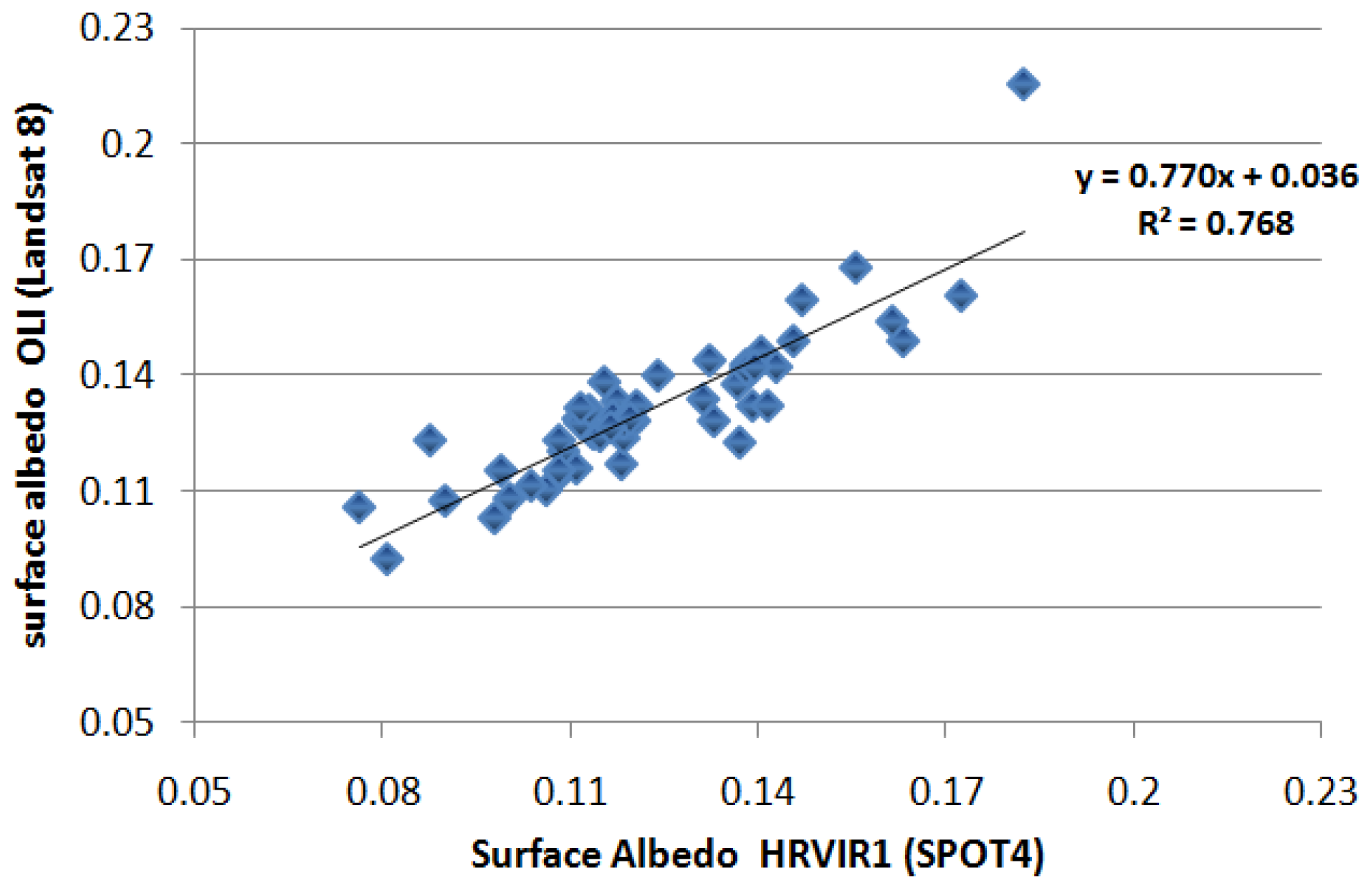
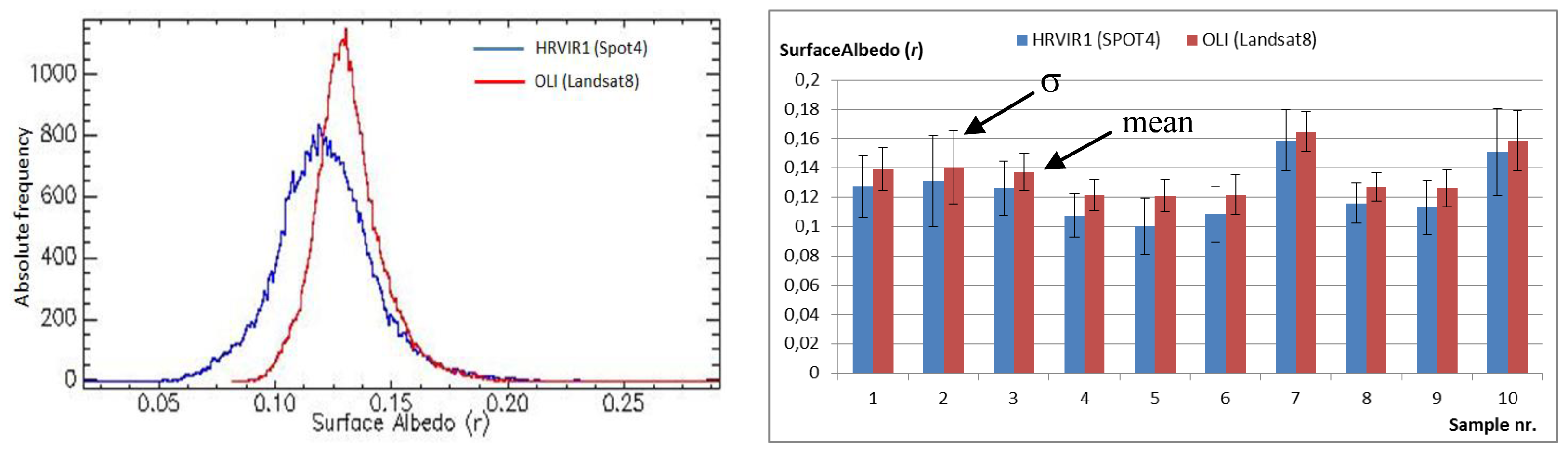
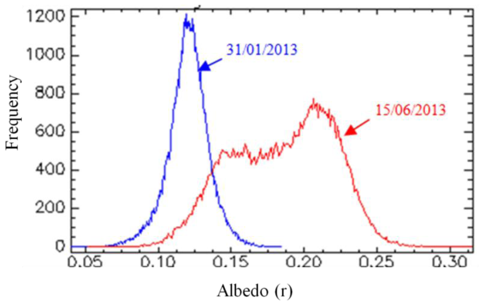
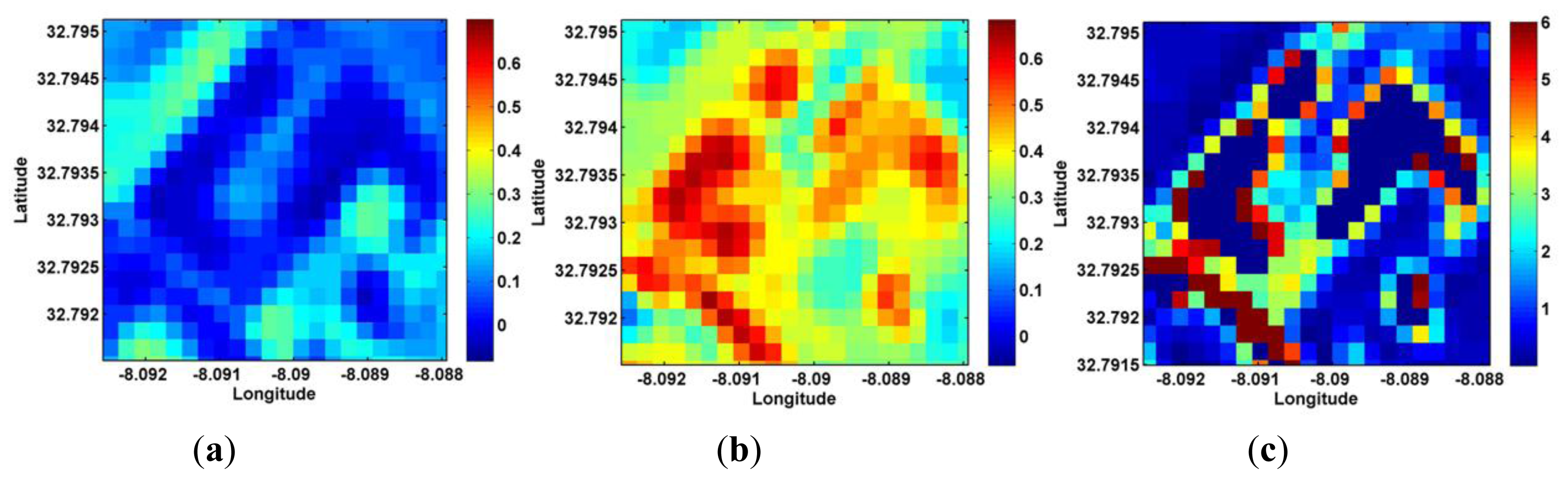
5.1.1. The Surface Albedo r
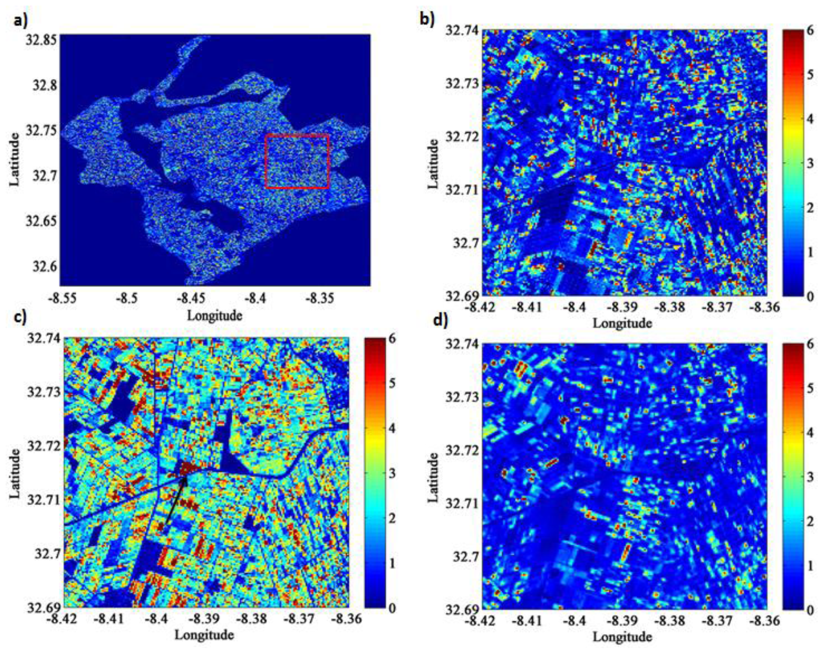
5.1.2. The Leaf Area Index (LAI)
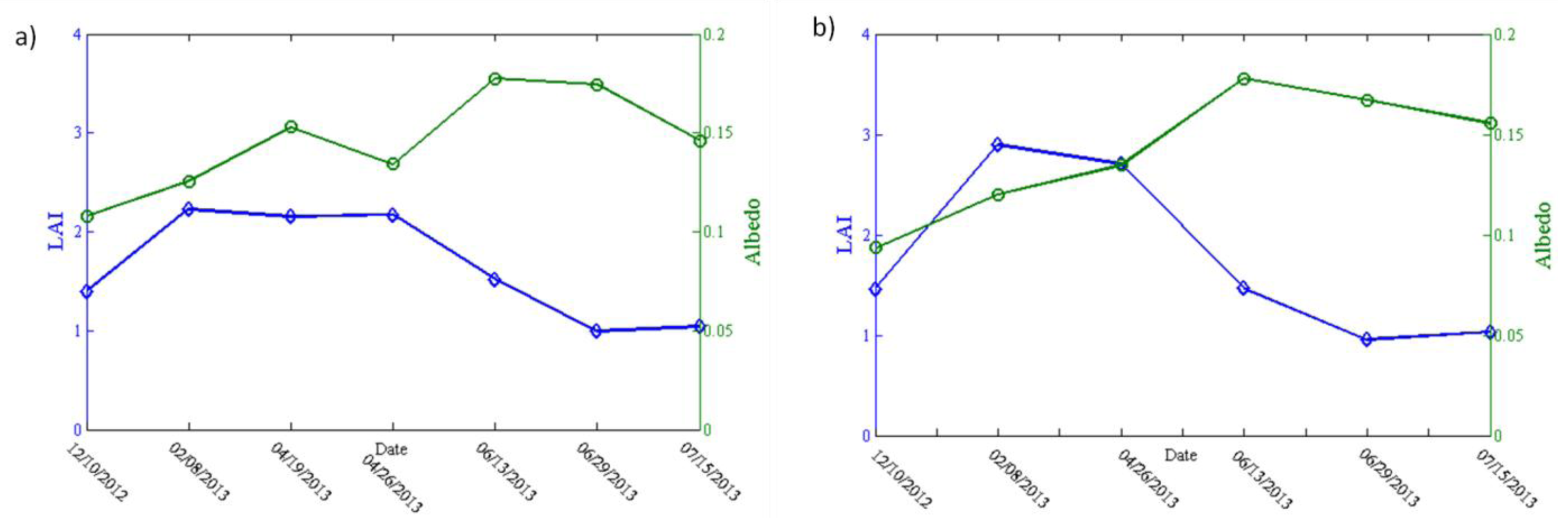
5.1.3. Soil Moisture and Radiation Control: LAI vs. Albedo
5.1.4. The Crop Height hc
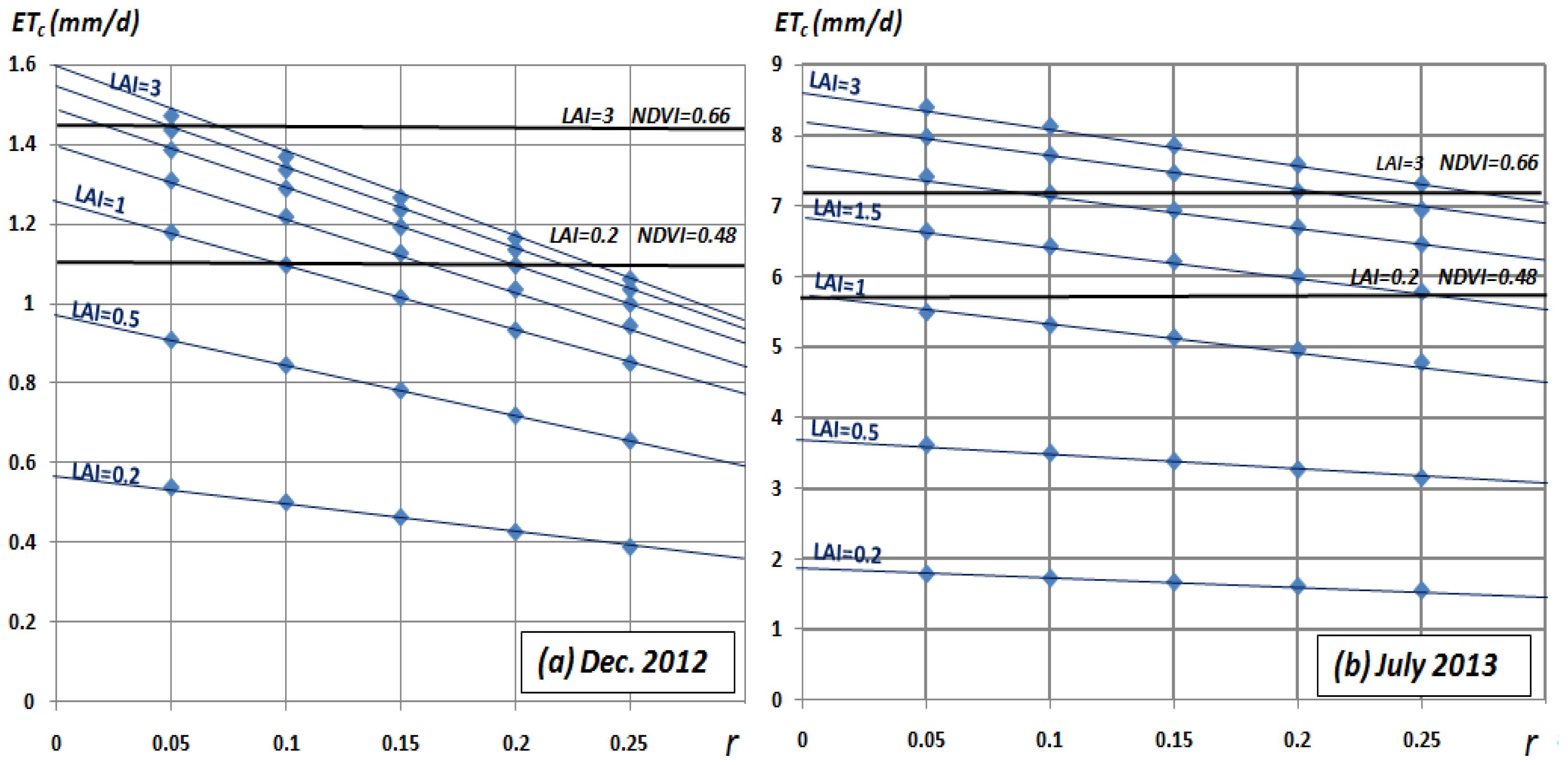
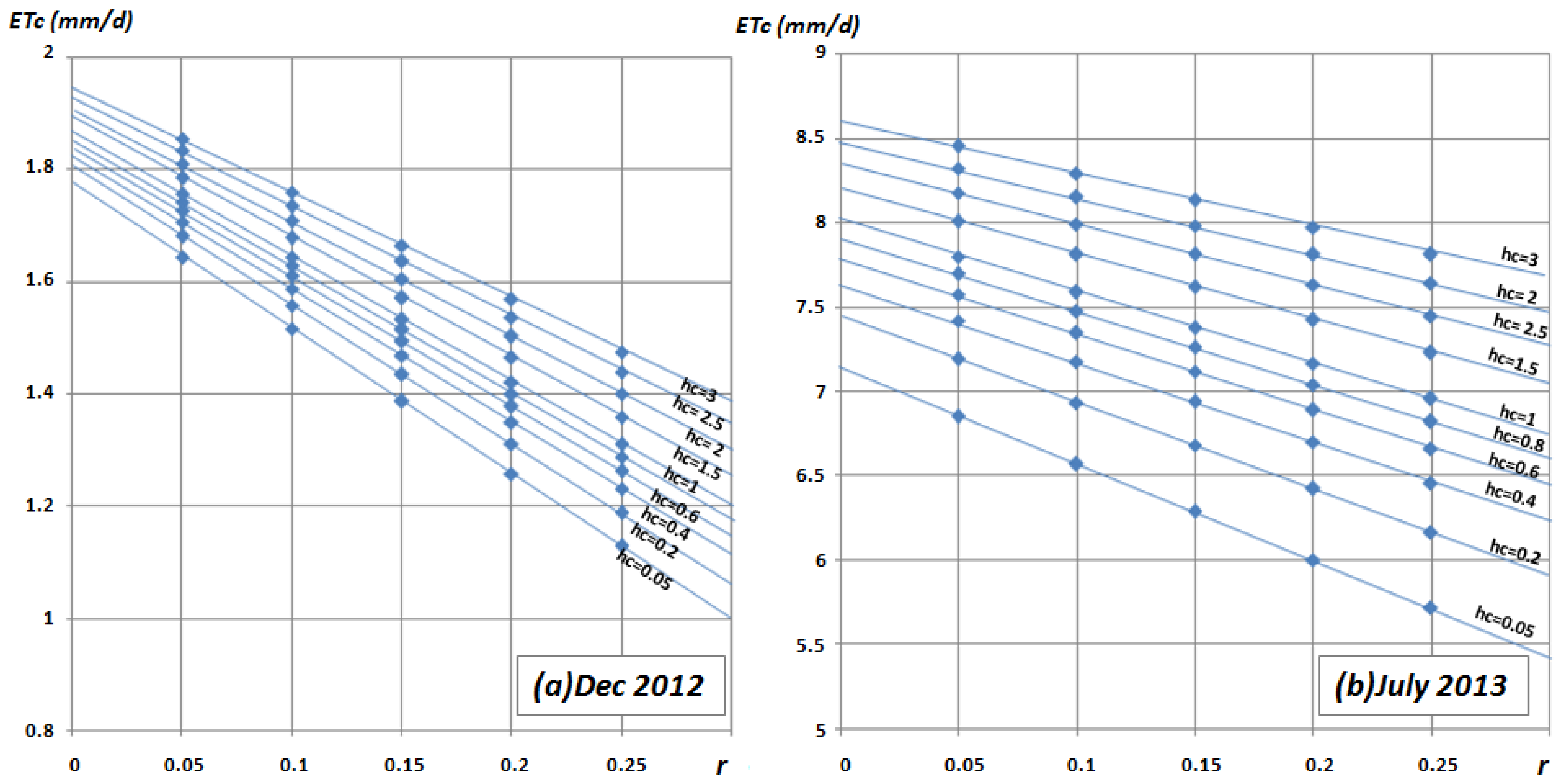
5.2. Sensitivity Analysis of ETc to Bio-Physical Variables
5.2.1. ETc (Analytical) versus (r-LAI)
5.2.2. ETc (Analytical) versus (r-hc)
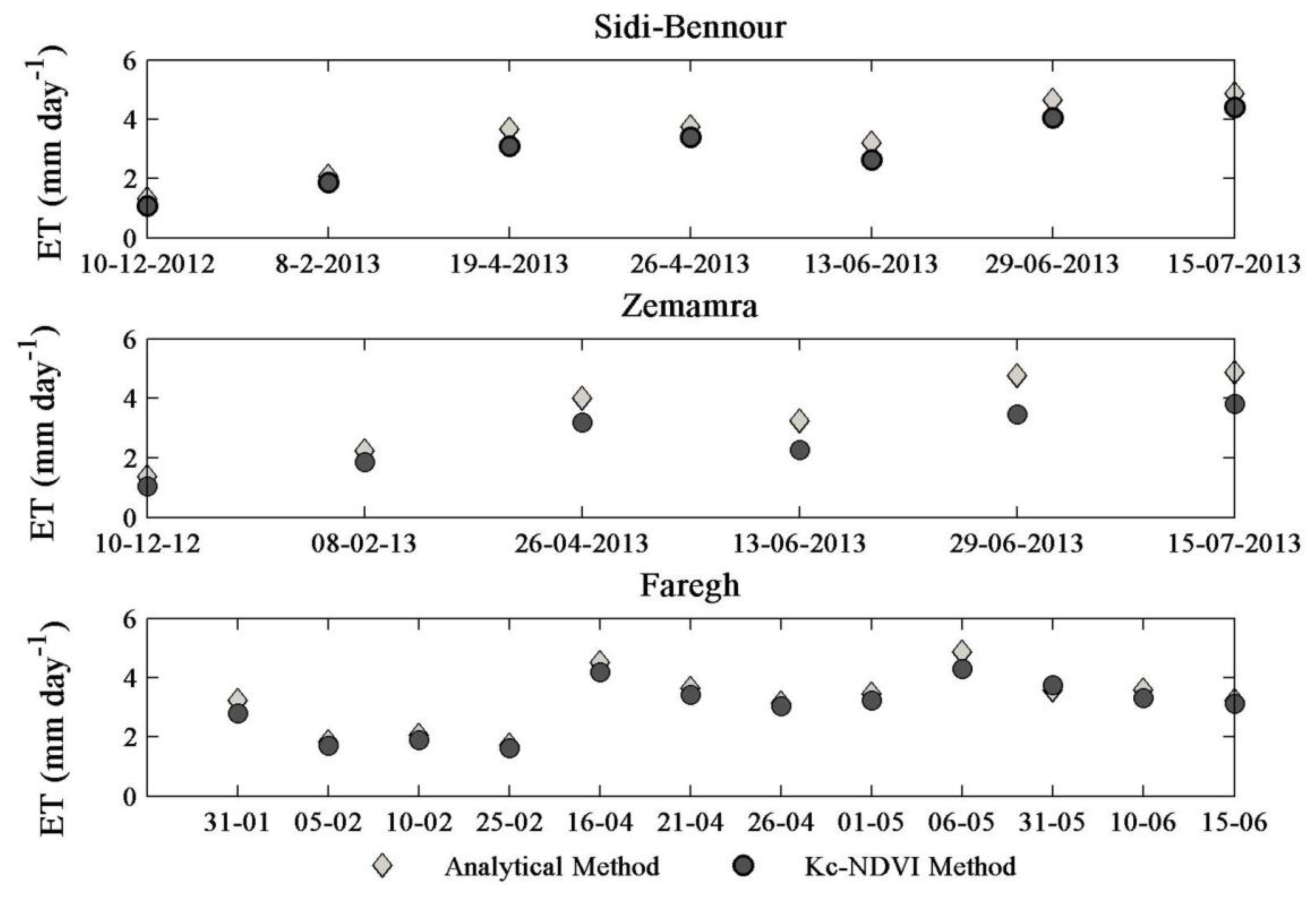
5.3. Estimation of Crop Evapotranspiration ETc: kc-NDVI vs. Analytical Approach
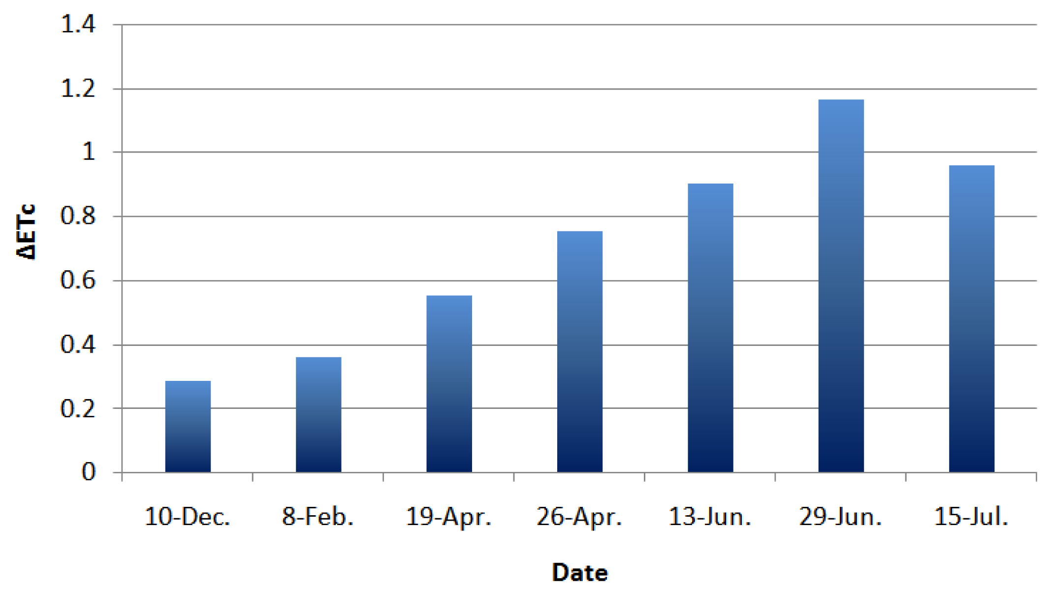
5.3.1. Temporal Variability
5.3.2. Spatial Variability
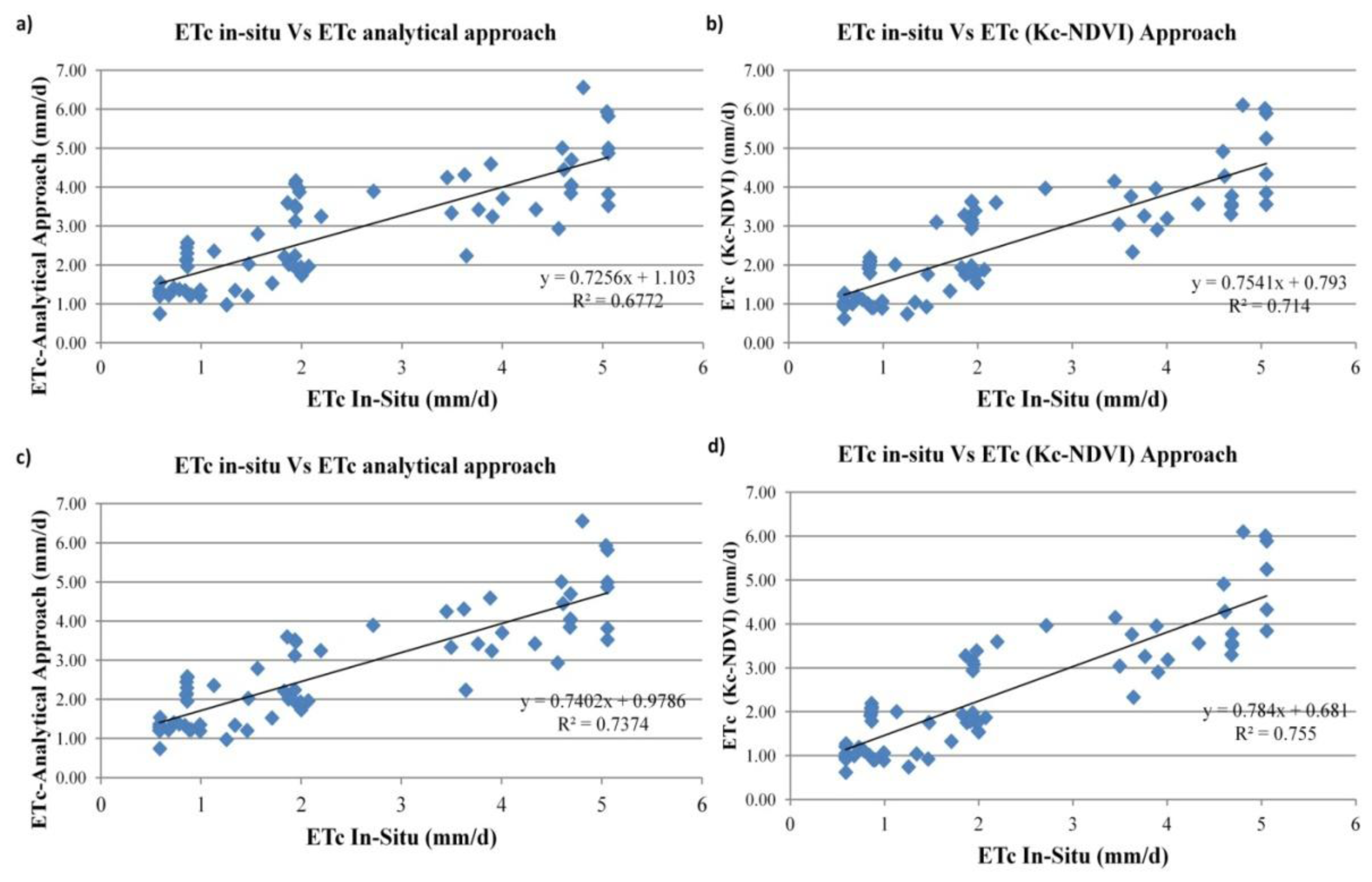
5.3.3. Validation
5.4. Irrigation Performance Indicator
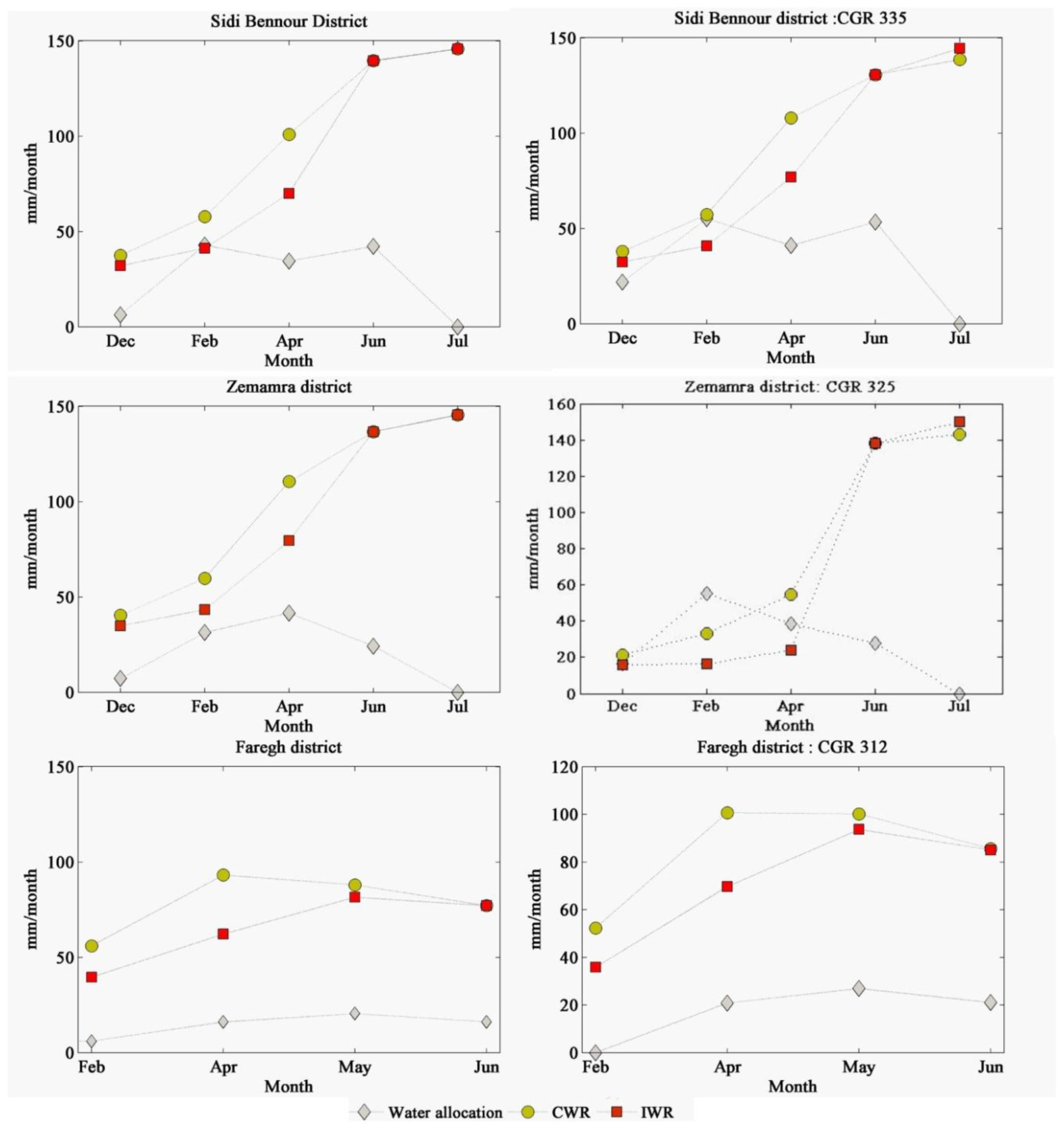
5.4.1. CWR and IWR versus Water Allocation
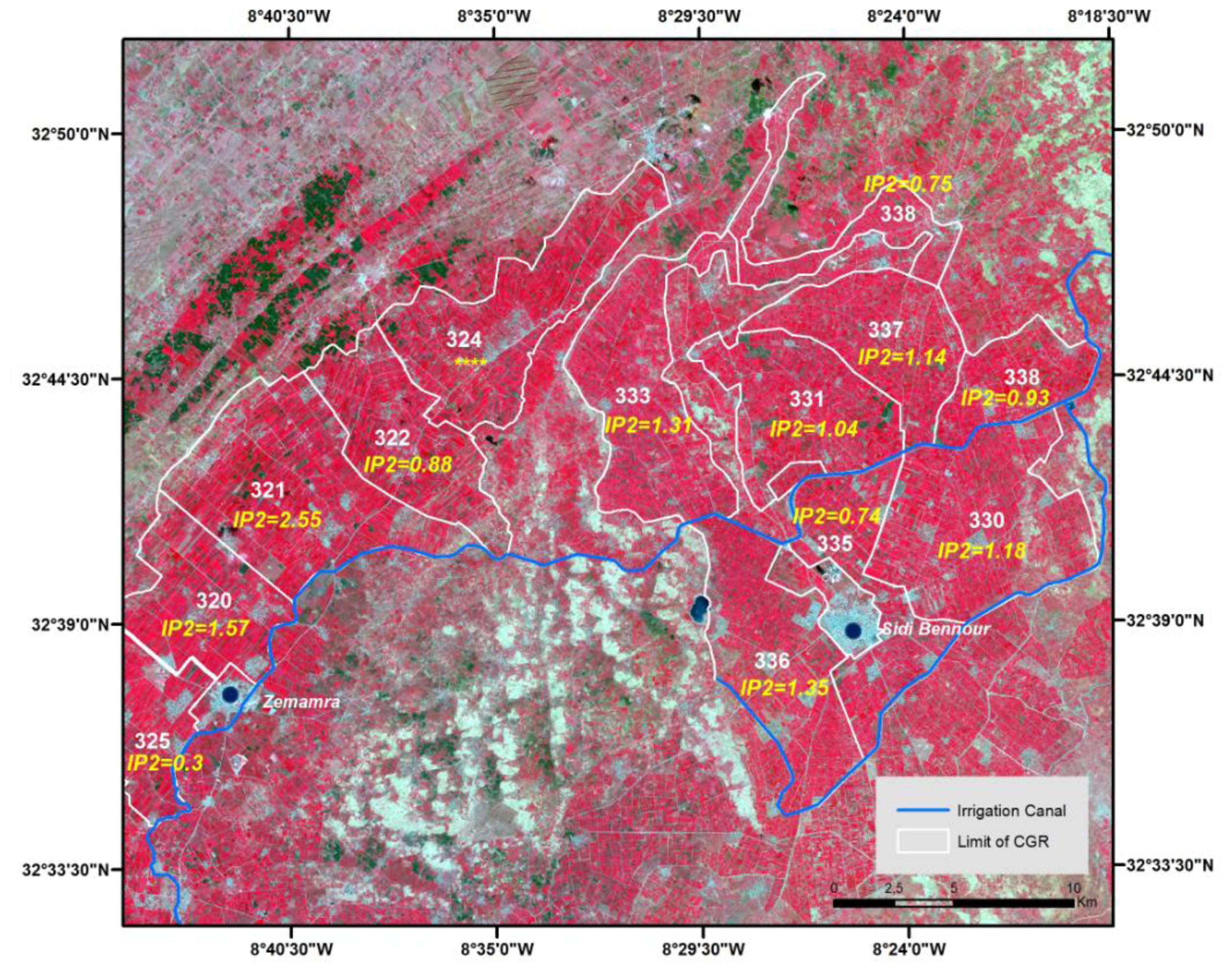
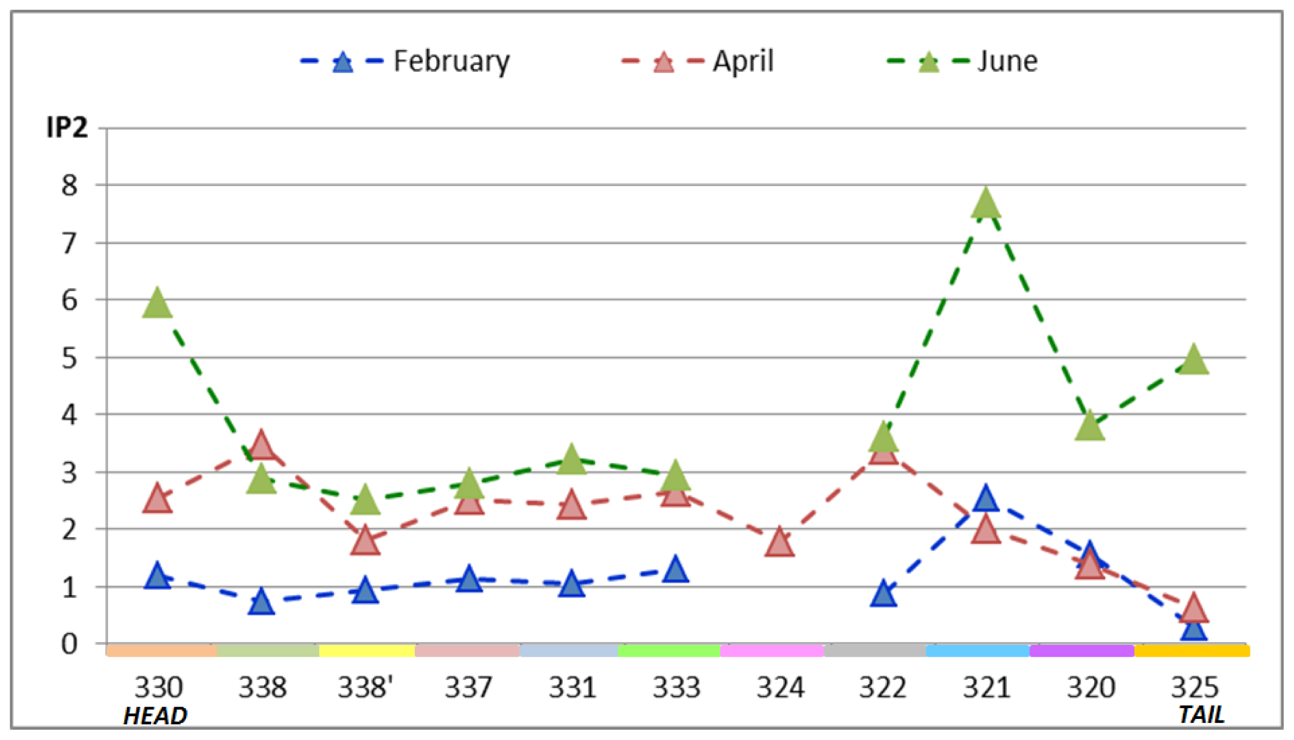
5.4.2. Spatial Distribution of IP2
6. Application in Irrigation Water Management
7. Conclusions
Acknowledgments
Conflicts of Interest
- Author ContributionsNadia Akdim was responsible for the study and the write up of the manuscript with contributions by Silvia Maria Alfieri and Massimo Menenti. Field data were acquired by Nadia Akdim, Adnane Habib, Abdeloihab Choukri and Kamal Labbassi. Field and satellite data were processed by Nadia Akdim, Silvia Maria Alfieri and Elijah Cheruiyot; and analyzed by Nadia Akdim, Silvia Maria Alfieri, Kamal Labbassi and Massimo Menenti.
References
- Lahlou, O.; Vidal, A. Remote Sensing and Management of Large Irrigation Projects. In Options Mediterraneennes. Serie A, Seminaires Mediterraneens, No. 4; Seminaires Mediterraneens: Montpellier, France, 1991; pp. 131–138. [Google Scholar]
- Vidal, A.; Sagardoy, J.A. Use of remote sensing techniques in irrigation and drainage. Water Rep 1995, 4, 173–178. [Google Scholar]
- Molden, D.J. Accounting for Water Use and Productivity. Available online: http://www.iwmi.cgiar.org/Publications/SWIM_Papers/PDFs/SWIM01.PDF (accessed on 18 February 2014).
- Molden, D.; Sakthivadivel, R. Water accounting to assess use and productivity of water. Int. J. Water Resour. Dev 1999, 15, 55–71. [Google Scholar]
- Menenti, M.; Visser, T.N.M.; Morabito, J.A.; Drovandi, A. Appraisal of Irrigation Performance with Satellite Data and Georeferenced Information. In Irrigation Theory and Practice; Rydzewsky, J.R., Ward, K., Eds.; Pentech Press: London, UK, 1989. [Google Scholar]
- Azzali, S. High and low resolution satellite images to monitor agricultural land. Rep. Winand Star. Cent. Wagening 1990, 61, 41–56. [Google Scholar]
- Moran, M.S.; Jackson, R.D. Assessing the spatial distribution of evapotranspiration using remotely sensed inputs. J. Environ. Qual 1991, 20, 725–737. [Google Scholar]
- Moran, M.S.; Inoue, Y.; Barnes, E.M. Opportunities and limitations for image-based remote sensing in precision crop management. Remote Sens. Environ 1997, 61, 319–346. [Google Scholar]
- Kustas, W.P.; Perry, E.M.; Doraiswamy, P.C.; Moran, M.S. Using satellite remote sensing to extrapolate evapotranspiration estimates in time and space over a semiarid rangeland basin. Remote Sens. Environ 1994, 49, 275–286. [Google Scholar]
- D’Urso, G.; Menenti, M. Section of Remote Sensing for agriculture, Forestry, and Natural Resources. In Mapping Crop Coefficients in Irrigated Areas from Landsat TM Images; International Society for Optics and Photonics: Paris, France, 1995; pp. 41–47. [Google Scholar]
- D’Urso, G. Operative Approaches to Determine Crop Water Requirements from Earth Observation Data: Methodologies and Applications. Proceedings of Earth Observation for Vegetation Monitoring and Water Management, Naples, Italy, 10–11 November 2005; pp. 14–25.
- Vuolo, F.; D’Urso, G.; Richter, K.; Prueger, J.; Kustas, W. Physically-Based Methods for the Estimation of Crop Water Requirements from EO Optical Data, 2008. Proceedings of Geosciences and Remote Sensing Symposium, IGARSS 2008, Boston, Massachusetts, USA, 8–11 July 2008; pp. IV-275–IV-278.
- Bastiaanssen, W.G.M.; Molden, D.J.; Makin, I.W. Remote sensing for irrigated agriculture: Examples from research and possible applications. Agric. Water Manag 2000, 46, 137–155. [Google Scholar]
- Er-Raki, S.; Chehbouni, A.; Guemouria, N.; Duchemin, B.; Ezzahar, J.; Hadria, R. Combining FAO-56 model and ground-based remote sensing to estimate water consumptions of wheat crops in a semi-arid region. Agric. Water Manag 2007, 87, 41–54. [Google Scholar]
- Er-Raki, S.; Chehbouni, A.; Duchemin, B. Combining satellite remote sensing data with the FAO-56 dual approach for water use mapping in irrigated wheat fields of a semi-arid region. Remote Sens 2010, 2, 375–387. [Google Scholar]
- Yang, Y.; Yang, Y.; Liu, D.; Nordblom, T.; Wu, B.; Yan, N. Regional water balance based on remotely sensed evapotranspiration and irrigation: An assessment of the Haihe Plain, China. Remote Sens 2014, 6, 2514–2533. [Google Scholar]
- Teixeira, A.H.D.C. Determining regional actual evapotranspiration of irrigated crops and natural vegetation in the São Francisco river basin (Brazil) using remote sensing and penman-monteith equation. Remote Sens 2010, 2, 1287–1319. [Google Scholar]
- Alexandridis, T.K.; Cherif, I.; Chemin, Y.; Silleos, G.N.; Stavrinos, E.; Zalidis, G.C. Integrated methodology for estimating water use in mediterranean agricultural areas. Remote Sens 2009, 1, 445–465. [Google Scholar]
- Bastiaanssen, W.G.M.; Thiruvengadachari, S.; Sakthivadivel, R.; Molden, D.J. Satellite remote sensing for estimating productivities of land and water. Int. J. Water Resour. Dev 1999, 15, 181–194. [Google Scholar]
- Bastiaanssen, W.G.M.; Bos, M.G. Irrigation performance indicators based on remotely sensed data: A review of literature. Irrig. Drain. Syst 1999, 13, 291–311. [Google Scholar]
- Zwart, S.J.; Bastiaanssen, W.G.M. Review of measured crop water productivity values for irrigated wheat, rice, cotton and maize. Agric. Water Manag 2004, 69, 115–133. [Google Scholar]
- Teixeira, A.D.C.; Bassoi, L.H. Crop water productivity in semi-arid regions: From field to large scales. Ann. Arid Zone 2009, 48, 1–13. [Google Scholar]
- Jackson, R.D.; Idao, S.B.; Reginato, R.J.; Pinter, P.J. Remotely Sensed Crop Temperatures and Reflectances as Inputs to Irrigtion Scheduling. Available online: http://cedb.asce.org/cgi/WWWdisplay.cgi?31647 (accessed on 18 February 2014).
- Jackson, R.D.; Idso, S.B.; Reginato, R.J.; Pinter, P.J., Jr. Canopy temperature as a crop water stress indicator. Water Resour. Res 1981, 17, 1133–1138. [Google Scholar]
- Jackson, R.D. Section of Remote Sensing: Critical Review if Technology. In Remote Sensing of Vegetation Characteristics for Farm Management; International Society for Optics and Photonics: Arlington, Washington, DC, USA, 1984; pp. 81–97. [Google Scholar]
- Makin, I.W. Applications of Remotely Sensed, Multi-Spectral Data in Monitoring Saline Soils; Irrigation and Power Research Institute (IPRI): Punjab, Amritsar, India, 1986. [Google Scholar]
- Ben-Asher, J.; Charach, C.; Zemel, A. Infiltration and water extraction from trickle irrigation source: The effective hemisphere model. Soil. Sci. Soc. Am. J 1986, 50, 882–887. [Google Scholar]
- Moran, M.S.; Clarke, T.R.; Inoue, Y.; Vidal, A. Estimating crop water deficit using the relation between surface-air temperature and spectral vegetation index. Remote Sens. Environ 1994, 49, 246–263. [Google Scholar]
- Er-Raki, S.; Chehbouni, A.; Hoedjes, J.; Ezzahar, J.; Duchemin, B.; Jacob, F. Improvement of FAO-56 method for olive orchards through sequential assimilation of thermal infrared-based estimates of ET. Agric. Water Manag 2008, 95, 309–321. [Google Scholar]
- Wolters, W. Influences on the Efficiency of Irrigation Water Use; International Institute for Land Reclamation and Improvement: Wageningen, the Netherlands, 1992. [Google Scholar]
- Murray-Rust, H.; Snellen, W.B. Irrigation System Performance Assessment and Diagnosis; Irrigation Water Management Institute: Colombo, Sri Lanka, 1993. [Google Scholar]
- Bos, M.G.; Wolters, W. Influences of Irrigation on Drainage. In Drainage Principles and Applications; Ritzema, H.P., Ed.; International Institute for Land Reclamation and Improvement: Wageningen, the Netherlands, 1994; pp. 513–531. [Google Scholar]
- Allen, R.G.; Pereira, L.S.; Raes, D.; Smith, M. Crop Evapotranspiration-Guidelines for Computing Crop Water Requirements-FAO Irrigation and Drainage Paper 56. Available online: http://www.kimberly.uidaho.edu/water/fao56/fao56.pdf (accessed on 18 February 2014).
- López-Urrea, R.; Martín de Santa Olalla, F.; Montoro, A.; López-Fuster, P. Single and dual crop coefficients and water requirements for onion (Allium cepa L.) under semiarid conditions. Agric. Water Manag 2009, 96, 1031–1036. [Google Scholar]
- Casa, R.; Russell, G.; Lo Cascio, B. Estimation of evapotranspiration from a field of linseed in central Italy. Agric. For. Meteorol 2000, 104, 289–301. [Google Scholar]
- Benli, B.; Kodal, S.; Ilbeyi, A.; Ustun, H. Determination of evapotranspiration and basal crop coefficient of alfalfa with a weighing lysimeter. Agric. Water Manag 2006, 81, 358–370. [Google Scholar]
- Paço, T.A.; Ferreira, M.I.; Conceição, N. Peach orchard evapotranspiration in a sandy soil: Comparison between eddy covariance measurements and estimates by the FAO 56 approach. Agric. Water Manag 2006, 85, 305–313. [Google Scholar]
- Er-Raki, S.; Chehbouni, A.; Guemouria, N.; Ezzahar, J.; Khabba, S.; Boulet, G.; Hanich, L. Citrus orchard evapotranspiration: Comparison between eddy covariance measurements and the FAO-56 approach estimates. Plant Biosyst 2009, 143, 201–208. [Google Scholar] [Green Version]
- Johnson, L.F.; Trout, T.J. Satellite NDVI assisted monitoring of vegetable crop evapotranspiration in California’s San Joaquin valley. Remote Sens 2012, 4, 439–455. [Google Scholar]
- De Bie, C.A.J.M.; Khan, M.R.; Smakhtin, V.U.; Venus, V.; Weir, M.J.C.; Smaling, E.M.A. Analysis of multi-temporal SPOT NDVI images for small-scale land-use mapping. Int. J. Remote Sens 2011, 32, 6673–6693. [Google Scholar]
- Benhadj, I.; Simonneaux, V.; Maisongrande, P.; Khabba, S.; Chehbouni, A. Combined Use of NDVI Time Courses at Low and High Spatial Resolution to Estimate Land Cover and Crop Evapotranspiration in Semi-Arid Areas. Proceedings of International Workshop on the Analysis of Multi-temporal Remote Sensing Images, 2007, MultiTemp 2007, Leuven, Belgium, 18–20 July 2007; pp. 1–6.
- Thenkabail, P.S.; Wu, Z. An Automated Cropland Classification Algorithm (ACCA) for Tajikistan by combining Landsat, MODIS, and secondary data. Remote Sens 2012, 4, 2890–2918. [Google Scholar]
- Amri, R.; Zribi, M.; Lili-Chabaane, Z.; Duchemin, B.; Gruhier, C.; Chehbouni, A. Analysis of vegetation behavior in a North African semi-arid region, using SPOT-VEGETATION NDVI data. Remote Sens 2011, 3, 2568–2590. [Google Scholar]
- Atzberger, C.; Rembold, F. Mapping the spatial distribution of winter crops at sub-pixel level using AVHRR NDVI time series and neural nets. Remote Sens 2013, 5, 1335–1354. [Google Scholar]
- Gumma, M.K.; Thenkabail, P.S.; Hideto, F.; Nelson, A.; Dheeravath, V.; Busia, D.; Rala, A. Mapping irrigated areas of Ghana using fusion of 30 m and 250 m resolution remote-sensing data. Remote Sens 2011, 3, 816–835. [Google Scholar]
- González-Dugo, M.P.; Escuin, S.; Cano, F.; Cifuentes, V.; Padilla, F.L.M.; Tirado, J.L.; Oyonarte, N.; Fernández, P.; Mateos, L. Monitoring evapotranspiration of irrigated crops using crop coefficients derived from time series of satellite images. II. Application on basin scale. Agric. Water Manag 2013, 125, 92–104. [Google Scholar]
- Conrad, C.; Fritsch, S.; Zeidler, J.; Rücker, G.; Dech, S. Per-field irrigated crop classification in arid central Asia using SPOT and ASTER data. Remote Sens 2010, 2, 1035–1056. [Google Scholar]
- Azzali, S.; Menenti, M. Mapping isogrowth zones on continental scale using temporal Fourier analysis of AVHRR-NDVI data. Int. J. Appl. Earth Obs. Geoinform 1999, 1, 9–20. [Google Scholar]
- Calera, A.B.; Jochum, A.M.; García, A.C.; Rodríguez, A.M.; Fuster, P.L. Irrigation management from space: Towards user-friendly products. Irrig. Drain. Syst 2005, 19, 337–353. [Google Scholar]
- D’Urso, G. Current status and perspectives for the estimation of crop water requirements from Earth Observation. Ital. J. Agron 2010, 5, 107–120. [Google Scholar]
- Rocha, J.; Perdigão, A.; Melo, R.; Henriques, C. Managing Water in Agriculture through Remote Sensing Applications. Proceedings of 30th EARSeL Symposium on Remote Sensing for Science, Education, and Natural and Cultural Heritage, Paris, France, 31 May–3 June 2010; pp. 223–230.
- Rouse, J.W.; Haas, R.H.; Schell, J.A.; Deering, D.W.; Harlan, J.C. Monitoring the Vernal Advancement and Retrogradation (Greenwave Effect) of Natural Vegetation; Texas Agricultural and Mecanical University, Remote Sensing Center: Texas, TX, USA, 1974. [Google Scholar]
- Richardson, A.J.; Weigand, C.L. Distinguishing vegetation from soil background information. Photogramm. Eng. Remote Sens 1977, 43, 1541–1552. [Google Scholar]
- Huete, A.R. A soil-adjusted vegetation index (SAVI). Remote Sens. Environ 1988, 25, 295–309. [Google Scholar]
- Ray, S.S.; Dadhwal, V.K. Estimation of crop evapotranspiration of irrigation command area using remote sensing and GIS. Agric. Water Manag 2001, 49, 239–249. [Google Scholar]
- Garatuza-Payan, J.; Tamayo, A.; Watts, C.; Rodríguez, J.C. Estimating Large Area Wheat Evapotranspiration from Remote Sensing Data. Proceedings of IEEE International Geoscience and Remote Sensing Symposium, 2003, IGARSS ’03, Toulouse, France, 21–25 July 2003; pp. 380–382.
- Gontia, N.K.; Tiwari, K.N. Estimation of crop coefficient and evapotranspiration of wheat (Triticum aestivum) in an irrigation command using remote sensing and GIS. Water Resour. Manag 2010, 24, 1399–1414. [Google Scholar]
- Clevers, J. Application of a weighted infrared-red vegetation index for estimating leaf area index by correcting for soil moisture. Remote Sens. Environ 1989, 29, 25–37. [Google Scholar]
- Pinty, B.; Verstraete, M.M. GEMI: A non-linear index to monitor global vegetation from satellites. Vegetatio 1992, 101, 15–20. [Google Scholar]
- Menenti, M.; Bastiaanssen, W.; Van Eick, D.; Abd el Karim, M.A. Linear relationships between surface reflectance and temperature and their application to map actual evaporation of groundwater. Adv. Space Res 1989, 9, 165–176. [Google Scholar]
- D’Urso, G.; Menenti, M.; Santini, A. Regional application of one-dimensional water flow models for irrigation management. Agric. Water Manag 1999, 40, 291–302. [Google Scholar]
- Ferré, M.; Ruhard, J.P. Les bassins des Abda-Doukkala et du Sahel de Azemmour à Safi. Notes Mém. Serv. Géol 1975, 23, 261–297. [Google Scholar]
- Guemimi, A. Plan D’action D’économie de L’eau Dans le Périmètre Des Doukkala. Proceedings of La Modernisation de L’agriculture Irriguée. Actes du Séminaire Euro-Méditerranéen, Thème 1: Aspects Techniques de la Modernisation des Systèmes Irriguès, Rabat, Maroc, 19–23 April 2004; pp. 1–10.
- Rahman, H.; Dedieu, G. SMAC: A simplified method for the atmospheric correction of satellite measurements in the solar spectrum. Int. J. Remote Sens 1994, 15, 123–143. [Google Scholar]
- Mousivand, A.; Menenti, M.; Gorte, B.; Verhoef, W. Global sensitivity analysis of the spectral radiance of a soil-vegetation system. Remote Sens. Environ 2014, 145, 131–144. [Google Scholar]
- Smith, M. CROPWAT: A Computer Program for Irrigation Planning and Management; Food and Agriculture Organization (FAO): Rome, Italy, 1992; Volume 46. [Google Scholar]
- Kashyap, P.S.; Panda, R.K. Evaluation of evapotranspiration estimation methods and development of crop-coefficients for potato crop in a sub-humid region. Agric. Water Manag 2001, 50, 9–25. [Google Scholar]
- Allen, R.G. Using the FAO-56 dual crop coefficient method over an irrigated region as part of an evapotranspiration intercomparison study. J. Hydrol 2000, 229, 27–41. [Google Scholar]
- Suleiman, A.A.; Tojo Soler, C.M.; Hoogenboom, G. Evaluation of FAO-56 crop coefficient procedures for deficit irrigation management of cotton in a humid climate. Agric. Water Manag 2007, 91, 33–42. [Google Scholar]
- Choudhury, B.J.; Ahmed, N.U.; Idso, S.B.; Reginato, R.J.; Daughtry, C.S.T. Relations between evaporation coefficients and vegetation indices studied by model simulations. Remote Sens. Environ 1994, 50, 1–17. [Google Scholar]
- Heilman, J.L.; Heilman, W.E.; Moore, D.G. Evaluating the crop coefficient using spectral reflectance. Agron. J 1982, 74, 967–971. [Google Scholar]
- Bausch, W.C.; Neale, C.M.U. Spectral inputs improve corn crop coefficients and irrigation scheduling. Trans. ASAE 1989, 32, 1901–1908. [Google Scholar]
- Neale, C.M.U.; Bausch, W.C.; Heermann, D.F. Development of reflectance-based crop coefficients for corn. Trans. ASAE 1989, 32, 1891–1900. [Google Scholar]
- Bausch, W.C. Remote sensing of crop coefficients for improving the irrigation scheduling of corn. Agric. Water Manag 1995, 27, 55–68. [Google Scholar]
- Bausch, W.C. Soil background effects on reflectance-based crop coefficients for corn. Remote Sens. Environ 1993, 46, 213–222. [Google Scholar]
- Simonneaux, V.; Duchemin, B.; Helson, D.; Er-Raki, S.; Olioso, A.; Chehbouni, A.G. The use of high-resolution image time series for crop classification and evapotranspiration estimate over an irrigated area in central Morocco. Int. J. Remote Sens 2008, 29, 95–116. [Google Scholar]
- Menenti, M.; Bastiaanssen, W.G.M.; van Eick, D. Determination of surface hemispherical reflectance with Thematic Mapper data. Remote Sens. Environ 1989, 28, 327–337. [Google Scholar]
- Vuolo, F.; Neugebauer, N.; Bolognesi, S.; Atzberger, C.; D’Urso, G. Estimation of leaf area index using DEIMOS-1 data: Application and transferability of a semi-empirical relationship between two agricultural areas. Remote Sens 2013, 5, 1274–1291. [Google Scholar]
- Menenti, M.; Ritchie, J.C. Estimation of effective aerodynamic roughness of Walnut Gulch watershed with laser altimeter measurements. Water Resour. Res 1994, 30, 1329–1337. [Google Scholar]
- Ritchie, J.C.; Menenti, M.; Weltz, M.A. Measurements of land surface features using an airborne laser altimeter: The HAPEX-Sahel experiment. Int. J. Remote Sens 1996, 17, 3705–3724. [Google Scholar]
- De Vries, A.C.; Kustas, W.P.; Ritchie, J.C.; Klaassen, W.; Menenti, M.; Rango, A.; Prueger, J.H. Effective aerodynamic roughness estimated from airborne laser altimeter measurements of surface features. Int. J. Remote Sens 2003, 24, 1545–1558. [Google Scholar]
- Payero, J.O.; Neale, C.M.U.; Wright, J.L. Comparison of eleven vegetation indices for estimating plant height of alfalfa and grass. Appl. Eng. Agric 2004, 20, 385–393. [Google Scholar]
- Brutsaert, W. Evaporation into the Atmosphere: Theory, History, and Applications; Reidel Dordrecht: Dordrecht, The Netherlands, 1982. [Google Scholar]
- Moran, M.S.; Jackson, R.D.; Hart, G.F.; Slater, P.N.; Bartell, R.J.; Biggar, S.F.; Gellman, D.I.; Santer, R.P. Obtaining surface reflectance factors from atmospheric and view angle corrected SPOT-1 HRV data. Remote Sens. Environ 1990, 32, 203–214. [Google Scholar]
- Su, Z.; Schmugge, T.; Kustas, W.P.; Massman, W.J. An evaluation of two models for estimation of the roughness height for heat transfer between the land surface and the atmosphere. J. Appl. Meteorol 2001, 40, 1933–1951. [Google Scholar]
- Jacob, F.; Olioso, A.; Gu, X.F.; Su, Z.; Seguin, B. Mapping surface fluxes using airborne visible, near infrared, thermal infrared remote sensing data and a spatialized surface energy balance model. Agronomie 2002, 22, 669–680. [Google Scholar]
- Perry, C.J. The IWMI water resources paradigm—Definitions and implications. Agric. Water Manag 1999, 40, 45–50. [Google Scholar]
- Rao, P.S. Review of Selected Literature on Indicators of Irrigation Performance. Available online: http://publications.iwmi.org/pdf/H_13467i.pdf (accessed on 18 February 2014).
- Nageswara Rao, P.P.; Mohankumar, A. Cropland inventory in the command area of Krishnarajasagar project using satellite data. Int. J. Remote Sens 1994, 15, 1295–1305. [Google Scholar]
- Menenti, M.; Azzali, S.; d’Urso, G. Management of Irrigation Schemes in Arid Countries. In Use of Remote Sensing Techniques in Irrigation and Drainage: Proceedings of the Expert Consultation; Food and Agricultural Organization (FAO): Montpellier, France, 1993; pp. 2–4. [Google Scholar]
- Bastiaanssen, W.G.M.; Pelgrum, H.; Droogers, P.; de Bruin, H.A.R.; Menenti, M. Area-average estimates of evaporation, wetness indicators and top soil moisture during two golden days in EFEDA. Agric. For. Meteorol 1997, 87, 119–137. [Google Scholar]
- Bastiaanssen, W.G.M.; Menenti, M.; Feddes, R.A.; Holtslag, A.A.M. A remote sensing surface energy balance algorithm for land (SEBAL). 1. Formulation. J. Hydrol 1998, 212, 198–212. [Google Scholar]
- Bos, M.G. Performance indicators for irrigation and drainage. Irrig. Drain. Syst 1997, 11, 119–137. [Google Scholar]
- Xu, D.; Guo, X. A study of soil line simulation from landsat images in mixed grassland. Remote Sens 2013, 5, 4533–4550. [Google Scholar]
- Duong, N.D.; Thoa, K.; Hoan, N.T. Some Advanced Techniques for SPOT 4 Xi Data Handling. Available online: http://www.geoinfo.com.vn/userfiles/file/cac%20cong%20trinh/15.pdf (accessed on 18 February 2014).
- Tomasko, M.G.; Doose, L.R.; Smith, P.H.; West, R.A.; Soderblom, L.A.; Combes, M.; Bézard, B.; Coustenis, A.; de Bergh, C.; Lellouch, E. The Descent Imager/Spectral Radiometer aboard Huygens. Available online: http://www.rssd.esa.int/SB/HUYGENS/docs/SP1177/tomask_1.pdf (accessed on 18 February 2014).
- Szafranek, I.; Amir, O.; Calahora, Z.; Adin, A.; Cohen, D. Blooming effects in indium antimode focal plane arrays. Proc. SPIE 1997, 3061, 633–639. [Google Scholar]
- Walker, D.; Epstein, H.; Jia, G.; Balser, A.; Copass, C.; Edwards, E.; Gould, W.; Hollingsworth, J.; Knudson, J.; Maier, H. Phytomass, LAI, and NDVI in northern Alaska: Relationships to summer warmth, soil pH, plant functional types, and extrapolation to the circumpolar Arctic. J. Geophys. Res. Atmos 2003, 108, 1984–2012. [Google Scholar]
- Feddes, R.A.; Kowalik, P.J.; Zaradny, H. Simulation Monographs. In Simulation of Field Water Use and Crop Yield; Centre for Agricultural Publishing and Documentation (PUDOC): Wageningen, The Netherlands, 1978; p. 188. [Google Scholar]
- Van Dam, J.; Huygen, J.; Wesseling, J.; Feddes, R.; Kabat, P.; van Walsum, P.; Groenendijk, P.; van Diepen, C. Theory of SWAP version 2.0; Simulation of water flow, solute transport and plant growth in the soil-water-atmosphere-plant environment. Tech. Doc 1997, 45, 970–973. [Google Scholar]
- TIGER. Avalable online: http://www.tiger.esa.int/PDF/news_45/20.pdf (accessed on 18 February 2014).
- Bos, M.G.; Nugteren, J. On Irrigation Efficiencies; International Institute for Land Reclamation and Improvement: Wageningen, The Netherlands, 1974; Volume 19. [Google Scholar]


| District | CGR | Area (Ha) | Irrigation System |
|---|---|---|---|
| SidiBennour | 330 | 5305.25 | Surface Irrigation |
| 331 | 3520.06 | ||
| 333 | 4293.39 | ||
| 335 | 3202.49 | ||
| 336 | 4197.1 | ||
| 337 | 3112.55 | ||
| 338 | 1738.92 | ||
| 338 sprinkler | 1905.3 | Sprinkler Irrigation | |
| Zemamra | 320 | 2995.18 | Sprinkler Irrigation |
| 321 | 5327.4 | ||
| 322 | 3243.68 | ||
| 324 | 4565.71 | ||
| 325 | 3122.27 | ||
| Faregh | 312 | 4840.24 | Drip Irrigation |
| 332 | 1490.46 | Surface Irrigation | |
| 310 | 4468.60 | ||
| 311 | 5021.25 | ||
| SENSOR | DATE | Area | SPECTRAL RESOLUTION (μm) | Spatial Resolution | ORBIT |
|---|---|---|---|---|---|
| SPOT4-HRVIR1 | From January to June 2013 | FAREGH | XS1: 0.500–0.590 | 20 m | Altitude:832 km revisit: 5 days |
| XS2: 0.610–0.680 | |||||
| XS3: 0.790–0.890 | |||||
| SWIR (HRVIR): 1.530–1.750 | |||||
| RapidEye-REIS | 10 December 2012
| ZEMAMRA SIDIBENNOUR | Blue: 0.440–0.510 | 5 m | Altitude:630 km revisit: Daily (off-nadir); 5.5 days (at nadir) |
| Green: 0.520–0.590 | |||||
| 8 February 2013 | Red: 0.630–0.685 | ||||
| Red-Edge: 0.690–0.730 | |||||
| NIR: 0.760–0.850 | |||||
| Landsat 8-OLI | 19 April 2013 | SIDIBENNOUR ZEMAMRA | Coastal/Aerosol: 0.433–0.453 | 30 m | Altitude:705 km revisit: 16 days |
| Blue: 0.450–0.515 | |||||
| 26 April 2013 | Green: 0.525–0.600 | ||||
| Red: 0.630–0.680 | |||||
| 13 June 2013 | NearInfrared: 0.845–0.885 | ||||
| SWIR: 1.560–1.660 | |||||
| 29 June 2013 | SWIR: 2.100–2.300 | ||||
| Cirrus: 1.360–1.390 | |||||
| 15 July 2013 | Panchromatic: 0.500–0.680 | 15 m | |||
| PARAMETER | VALUE | Date |
|---|---|---|
| Model Atmosphere | Mid Latitude Summer | 10 December 2012 |
| 8 February 2013 | ||
| 19 April 2013 | ||
| 26 April 2013 | ||
| Tropical | 13 June 2013 | |
| 29 June 2013 | ||
| 15 July 2013 | ||
| Aerosol Model | Rural | |
| Aerosol Retrieval | None | |
| Visibility | 40 km (Default) | |
| Ground Altitude Above Sea Level | 150 m |
| Sensor | Spectral Band (μm) | Weighting Coefficient Wλ |
|---|---|---|
| RapidEye (REIS) | Blue: 0.440–0.510 | 0.2455 |
| Green: 0.520–0.590 | 0.2989 | |
| Red: 0.630–0.685 | 0.1973 | |
| NIR: 0.760–0.850 | 0.2583 | |
| Landsat 8 (OLI) | Blue: 0.450–0.515 | 0.2935 |
| Green: 0.525–0.600 | 0.2738 | |
| Red: 0.630–0.680 | 0.233 | |
| NIR: 0.845–0.885 | 0.1554 | |
| SWIR: 1.560–1.660 | 0.0322 | |
| SWIR: 2.100–2.300 | 0.0121 | |
| Spot 4 (HRVIR1) | XS1: 0.500–0.590 | 0.3925 |
| XS2: 0.610–0.680 | 0.3339 | |
| XS3: 0.790–0.890 | 0.224 | |
| SWIR:1.530–1.750 | 0.0496 | |
| Kc-NDVI Approach | Analytical Approach | ||||
|---|---|---|---|---|---|
| Mean | Standard Deviation | Mean | Standard Deviation | ||
| 20 × 20 | December | 1.22 | 0.25 | 1.47 | 0.55 |
| April | 4.06 | 0.74 | 4.08 | 0.90 | |
| June | 4.22 | 0.76 | 4.24 | 0.92 | |
| 200 × 200 | December | 1.26 | 0.36 | 1.55 | 0.74 |
| April | 4.58 | 0.72 | 4.78 | 1.08 | |
| June | 4.43 | 1.08 | 4.61 | 1.31 | |
© 2014 by the authors; licensee MDPI, Basel, Switzerland This article is an open access article distributed under the terms and conditions of the Creative Commons Attribution license (http://creativecommons.org/licenses/by/3.0/).
Share and Cite
Akdim, N.; Alfieri, S.M.; Habib, A.; Choukri, A.; Cheruiyot, E.; Labbassi, K.; Menenti, M. Monitoring of Irrigation Schemes by Remote Sensing: Phenology versus Retrieval of Biophysical Variables. Remote Sens. 2014, 6, 5815-5851. https://doi.org/10.3390/rs6065815
Akdim N, Alfieri SM, Habib A, Choukri A, Cheruiyot E, Labbassi K, Menenti M. Monitoring of Irrigation Schemes by Remote Sensing: Phenology versus Retrieval of Biophysical Variables. Remote Sensing. 2014; 6(6):5815-5851. https://doi.org/10.3390/rs6065815
Chicago/Turabian StyleAkdim, Nadia, Silvia Maria Alfieri, Adnane Habib, Abdeloihab Choukri, Elijah Cheruiyot, Kamal Labbassi, and Massimo Menenti. 2014. "Monitoring of Irrigation Schemes by Remote Sensing: Phenology versus Retrieval of Biophysical Variables" Remote Sensing 6, no. 6: 5815-5851. https://doi.org/10.3390/rs6065815