


Highlights
What are the main findings?
- Random Forest (RF) and Gradient Tree Boosting (GTB) achieved the highest accuracy (OA ≈ 92–93%, Kappa ≈ 0.91), significantly outperforming an unconstrained Classification and Regression Trees (CART) under family-wise correction and a linear-kernel Support Vector Machine (SVM) under false-discovery-rate control.
- Class-specific SHAP identified Normalized Difference Water Index (NDWI), Modified Normalized Difference Water Index (MNDWI), Normalized Difference Vegetation Index (NDVI), and KOMPSAT-3 NIR/blue bands as key drivers of water, forest, and vegetation classification.
- A leave-one-sensor-out (LOSO) ablation indicated that KOMPSAT-3 and Sentinel-2 provided additional predictive information, although no individual ablation contrast remained significant after multiplicity correction.
What are the implications of the main findings?
- Class-level SHAP combined with sensor-group ablation supports application-specific sensor selection: NDWI/MNDWI and the KOMPSAT-3 NIR/blue bands for water-resource monitoring, and the Sentinel-2 reflectance–index ensemble for bare land and mixed-area mapping, where the ablation effect is largest.
- Coupling SHAP with LOSO demonstrates how sensor-level necessity can diverge from feature-level attribution when information is shared among correlated inputs.
- Co-registering and fusing high-resolution KOMPSAT-3/5 with medium-resolution Sentinel-1/2 on a common 2.8 m analysis grid within a unified GEE-based XAI workflow provides a transferable template for an explainable multi-sensor data-cube design.
Abstract
This study benchmarks four classifiers—Random Forest (RF), Classification and Regression Trees (CART), Support Vector Machine (SVM), and Gradient Tree Boosting (GTB)—on an identical 16-feature KOMPSAT-3/5 and Sentinel-1/2 stack harmonized to a common 2.8 m grid within Google Earth Engine. RF and GTB reached overall accuracies of 92.4% and 92.8%, separating them from the unconstrained CART under family-wise correction and from the linear-kernel SVM under false-discovery-rate control. Class-specific SHAP was cross-interpreted against permutation importance, feature-correlation analysis, and a leave-one-sensor-out (LOSO) ablation, with SHAP and permutation-importance rankings in broad agreement (Spearman ρ = 0.72–0.92). The central contribution is to characterize two conditions—strong within-sensor collinearity and class-conditional information concentration—under which feature-level attribution and sensor-level necessity diverge. In the Bare Land class, no individual Sentinel-2 SWIR band ranks among the top three by SHAP, yet withholding the Sentinel-2 group produces the largest class-wise degradation observed (ΔF1 = 0.102 for RF and 0.130 for GTB), consistent with attribution dilution across the collinear SWIR1–SWIR2 pair (r = 0.97). Because none of the sixteen ablation contrasts survives multiplicity correction with a sample size of 250 (n = 250), these contrasts are reported as effect-size estimates rather than confirmatory tests.
1. Introduction
Recent studies have highlighted the growing importance of explainable artificial intelligence (XAI) in Earth Observation (EO) and remote sensing applications. Gevaert [1] argued that XAI in EO should not only aim to improve model accuracy but also enhance social and policy trust, increase accountability, and facilitate scientific discovery. However, achieving these broader objectives remains a critical challenge for improving the reliability and practical usability of XAI models. The following review situates the present study within recent XAI research in EO and identifies the specific gap it addresses.
Ishikawa et al. [2] proposed a case-based XAI framework for evaluating the reliability of deep learning (DL)-based remote sensing classification and demonstrated its complementary role alongside feature-attribution methods such as SHapley Additive exPlanations (SHAP) and Local Interpretable Model-agnostic Explanations (LIME). Similarly, Temenos et al. [3] integrated SHAP into a deep-learning framework for land-use/land-cover (LULC) classification and demonstrated that SHAP-based explanations improve model interpretability and user trust without compromising predictive performance. Chen et al. [4] further developed an interactive XAI tool for land-cover mapping in Google Earth Engine (GEE), providing both sample-level and class-level SHAP interpretations. Talukdar et al. [5] compared six machine learning (ML) classifiers for Landsat-based LULC mapping and reported that the Random Forest (RF) scheme achieved the highest overall classification accuracy, showing the strongest agreement with both index-based validation and field observations derived from Google Earth imagery.
Höhl et al. [6,7] surveyed XAI in EO, identifying SHAP, LIME, and Gradient-weighted Class Activation Mapping (Grad-CAM) as the most widely adopted methods and advocating inherently interpretable architectures, quantitative evaluation protocols, and integration with physical modeling and uncertainty analysis. Model-agnostic attribution has since been applied across data-scarce and thematic settings: Lee et al. [8] report that SHAP and LIME improve interpretability in few-shot remote sensing learning, while Lu et al. [9] combine RF with SHAP for desert classification, quantifying feature contributions at both global and local levels.
Comparative evaluations of XAI methods have also received attention beyond EO-specific applications: Van Zyl et al. [10] show that SHAP and Grad-CAM improve both predictive accuracy and computational efficiency in energy-demand forecasting by identifying redundant variables, and SHAP-, Grad-CAM- and RF-based frameworks have since been applied to flood-susceptibility mapping, wildfire-spread prediction, and soil-moisture estimation [11,12,13]. Collectively, these studies establish XAI as a standard component of AI-driven Earth observation.
More recently, Earth observation research has increasingly adopted remote sensing foundation models that learn transferable spatial, temporal, and multimodal representations from large-scale pretraining datasets, including Prithvi-EO-2.0 [14], SkySense V2 [15] and AlphaEarth Foundations [16]. Because such representations integrate optical, SAR, and other geospatial sources rather than treating each sensor independently, the question of which modality is actually necessary for a given prediction becomes correspondingly harder to answer from attribution alone. These models are cited here to motivate that question; they are not evaluation targets of the present study, which is conducted entirely at the conventional multi-sensor machine-learning level. The SHAP–LOSO framework proposed below addresses the question at that level and provides a conceptually transferable basis for interpreting multimodal and foundation-model-based systems. They are not evaluation targets of the present study, which is conducted entirely at the conventional multi-sensor machine-learning level. The SHAP–LOSO framework proposed below addresses this question at that level and provides a conceptually transferable basis for interpreting multimodal and foundation-model-based systems.
Accurate land-cover information underpins environmental monitoring, water-resource management, and urban and agricultural planning. Classifications based on a single sensor or a single acquisition date nevertheless remain constrained by sensor-specific limitations—atmospheric sensitivity, limited spatial resolution, and differences in sensing mechanism—and these constraints are most pronounced in heterogeneous landscapes where water, forest, cropland, and bare surfaces occur in close spatial proximity.
To overcome these limitations, recent studies have increasingly adopted multi-sensor approaches that integrate optical imagery with synthetic aperture radar (SAR) data by exploiting the differing physical bases of the two sensing mechanisms. Optical imagery provides rich spectral information describing the biophysical and biochemical properties of vegetation, water, and soil surfaces, whereas SAR observations are sensitive to surface roughness and structural characteristics and can be acquired regardless of cloud cover or illumination conditions. Furthermore, integrating medium-resolution Sentinel imagery with high-resolution KOMPSAT data combines broad spatial coverage with detailed local-scale information, making this approach particularly suitable for operational land-cover mapping that requires both regional consistency and fine spatial detail. Nevertheless, studies that simultaneously integrate high- and medium-resolution optical and SAR data while systematically analyzing their respective contributions within an XAI framework remain relatively scarce.
Nonlinear classifiers—Random Forests (RF), Classification and Regression Trees (CART), Support Vector Machines (SVM), and Gradient Tree Boosting (GTB)—are now widely used for land-cover classification. Conventional feature-importance measures, however, provide only a global variable ranking and explain neither how individual features contribute to specific classes nor how feature interactions shape predictions, which limits their use for sensor selection, feature-space design, and mission planning.
Within this context, SHAP, which decomposes individual predictions into feature-level contributions grounded in cooperative game theory, has emerged as a powerful framework for interpreting complex ML models. SHAP enables the quantitative assessment of how individual sensor bands or spectral indices influence class predictions at the pixel level by decomposing each prediction into additive feature-level contributions. Furthermore, visualization techniques such as beeswarm, waterfall, and dependency plots facilitate the interpretation of feature interactions and class-specific decision behavior. In remote sensing, however, SHAP has been applied predominantly to single-sensor datasets or to relatively limited feature sets.
Recent ML applications to multi-source LULC classification converge on a broadly consistent picture. RF achieved the highest accuracy in Sentinel-2-based GEE mapping [17], whereas Shao et al. [18] report the opposite ordering for urban land-cover, with eXtreme Gradient Boosting (XGBoost) outperforming both RF and Google Dynamic World, highlighting boosting’s advantages for multi-sensor mapping. RF was again the strongest performer in fused Landsat-8/Sentinel-1 tree-species mapping—where a SHAP analysis identified elevation and vegetation indices as the most influential variables [19]—and in multi-temporal Landsat monitoring, where GTB and CART showed greater temporal variability [20]; further comparisons confirm that RF and GTB generally provide robust performance across diverse environmental conditions [21,22]. Taken together, these studies do not converge on a single best algorithm: the reported ordering depends on the sensor configuration, the class scheme, and the study area, with RF favored in several Sentinel-based settings [17,19] and gradient boosting favored in others [18]. The present study accordingly does not set out to establish the superiority of any one classifier, but to characterize how four structurally distinct classifiers encode an identical multi-sensor feature space and how that encoding is reflected in their attributions. Lee et al. [23] presented an integrated SHAP–remove-and-retrain (ROAR)–bootstrap framework that quantifies and validates class-dependent sensor contributions in RF-based multi-sensor land-cover classification, enhancing interpretability while maintaining high accuracy. This study is methodologically distinct from our earlier RF-only SHAP–ROAR analysis [23] in three respects: (i) it compares four structurally distinct classifier families under an identical feature space and a fixed untuned hyperparameter configuration, rather than interpreting a single model; (ii) it validates attribution at the sensor-group level through a leave-one-sensor-out (LOSO) ablation, rather than at the individual-feature level through remove-and-retrain; and (iii) it addresses a different study area and a different class scheme. No accuracy figures, attribution values, or figures are reproduced from [23]; the two studies are complementary rather than incremental. Critically, the two protocols answer different questions: remove-and-retrain quantifies the faithfulness of a feature-level attribution, whereas LOSO quantifies the marginal predictive information of an entire acquisition modality, and the latter cannot be recovered by aggregating the former across the features of a sensor group.
Two gaps therefore remain. First, multi-sensor XAI studies in remote sensing typically either vary the input data while retaining a single classifier—most commonly RF—or compare several classifiers on predictive accuracy alone, without examining how structurally different algorithms encode identical evidence at the attribution level. Second, where attribution is reported, it is rarely validated against an independent, attribution-free criterion; therefore, feature importance obtained under strong inter-sensor collinearity is difficult to read as evidence of sensor necessity. This study addresses both gaps by benchmarking four structurally distinct classifiers on an identical high- and medium-resolution optical–SAR feature set and by cross-interpreting the resulting class-specific SHAP attributions against a LOSO ablation.
The present study is therefore distinguished from existing approaches on four dimensions: it compares four structurally distinct classifiers rather than varying the inputs under a single one; it combines high-resolution KOMPSAT-3 optical and KOMPSAT-5 SAR data with medium-resolution Sentinel-1 and Sentinel-2 observations on a common analysis grid; it validates the resulting attributions against criteria that are independent of the attribution method itself, namely permutation importance, the feature-correlation structure, and a sensor-group ablation; and it performs that validation at the level of the sensor group rather than the individual feature. The last of these also distinguishes the study from our earlier remove-and-retrain analysis [23], which operates at the feature level and quantifies attribution faithfulness, whereas the leave-one-sensor-out design used here quantifies the marginal predictive information of an entire acquisition modality.
The specific objectives of this study are as follows.
- (1)
- To construct an integrated multi-sensor feature space by combining high-resolution KOMPSAT-3 optical imagery, KOMPSAT-5 SAR data, Sentinel-1 SAR data, Sentinel-2 multispectral imagery, and derived spectral indices (Normalized Difference Water Index (NDWI), the Modified Normalized Difference Water Index (MNDWI), the Normalized Difference Vegetation Index (NDVI)) within a GEE workflow, and to evaluate land-cover classification performance for the Water, Forest, Vegetation, Bare Land, and Unclassified classes.
- (2)
- To benchmark four representative ML classifiers (RF, CART, SVM, and GTB) under identical multi-sensor inputs and fixed, untuned hyperparameter settings, and to compare them using overall accuracy (OA), the Kappa coefficient, class-wise F1-scores with bootstrap confidence intervals, and paired McNemar tests evaluated on a common validation partition.
- (3)
- To apply SHAP-based explainable AI at both the global (mean |SHAP|) and class-specific levels (beeswarm, waterfall, and dependency plots) to quantify sensor-, band-, and index-level contributions for each classifier and land-cover class, and to translate these findings into site-specific, evidence-based guidance for sensor and feature selection in multi-sensor data-cube designs.
- (4)
- To characterize the conditions under which feature-level attribution and sensor-level necessity diverge, treating such divergences as diagnostic evidence rather than as inconsistencies to be reconciled.
2. Materials and Methods
2.1. Study Area
This study was conducted in a compact regional study area characterized by heterogeneous land-cover types, including water bodies, forests, vegetated agricultural land, bare surfaces, and mixed or unclassified areas. Such spatial heterogeneity provides a suitable test bed for evaluating the applicability of multi-sensor land-cover classification methods.
The study area comprises water bodies embedded within predominantly forested mountainous terrain, whereas agricultural and vegetated areas are distributed across relatively flat lowlands. Figure 1 presents the study area used for the multi-sensor land-cover classification and SHAP-based interpretability analyses, together with the spatial coverage of the satellite datasets employed in this study. The study area is located in Hapcheon-gun, Gyeongsangnam-do, in the inland southeastern region of the Republic of Korea, and is defined by a rectangular boundary with corner coordinates of 127.980841°E, 35.646149°N (upper left); 127.980841°E, 35.534320°N (lower left); 128.148181°E, 35.646149°N (upper right); and 128.148181°E, 35.534320°N (lower right).
Figure 1.
Study area and spatial coverage of the multi-sensor datasets used in this study, including KOMPSAT-3, KOMPSAT-5, Sentinel-1, and Sentinel-2, overlaid on the base map with geographic coordinates and scale bar.
The region encompasses several inland water bodies of varying sizes, surrounded by diverse land-cover types. Topographically, it is characterized by complex terrain with pronounced elevation gradients and irregular slopes, which may introduce terrain shadow effects and mixed-pixel artifacts in optical imagery. These characteristics pose significant challenges for land-cover classification and underscore the importance of integrating optical and SAR data to enhance class discrimination across varying surface and illumination conditions. The study area was selected to ensure overlapping spatial coverage of KOMPSAT-3, KOMPSAT-5, Sentinel-1, and Sentinel-2 acquisitions within a comparable acquisition period.
2.2. Applied Methods
Figure 2 presents the overall workflow of the proposed framework, encompassing data acquisition, preprocessing, model training, accuracy assessment, and two complementary explainability analyses using Sentinel-1 SAR, Sentinel-2, KOMPSAT-3, and KOMPSAT-5 datasets. The upper part of the workflow illustrates the acquisition of optical imagery from KOMPSAT-3 and SAR observations from KOMPSAT-5 over the study area, together with Sentinel-1 SAR Ground Range Detected (GRD) and Sentinel-2 optical imagery. This multi-sensor configuration combines high-resolution domestic satellite data with medium-resolution Sentinel observations within a unified analysis framework.
Figure 2.
Overall workflow of the multi-sensor land-cover classification framework, encompassing GEE-based data preprocessing, four-classifier training (RF, CART, SVM, GTB), and accuracy assessment. Accuracy assessment branches into two parallel interpretability pathways—SHAP-based explainable AI and LOSO ablation—whose findings are cross-interpreted to assess the consistency and divergence between feature-level attribution and sensor-level necessity (dashed line). The same workflow is stated in algorithmic form as Algorithm A1 (Appendix A).
At the center of the workflow, GEE serves as the primary platform for acquiring and preprocessing Sentinel datasets via the GEE Application Programming Interface (API). The KOMPSAT-3 and KOMPSAT-5 datasets are first registered, mosaicked, and clipped to the study area boundary. Subsequently, data from all four sensors are resampled to a common spatial resolution, and the spectral indices NDVI, NDWI, and MNDWI are derived. These datasets are then integrated into a spatially consistent 2.8 m data cube, which serves as the input feature set for subsequent ML analyses.
The lower part of the workflow illustrates the four ML classifiers evaluated in this study: RF, CART, SVM, and GTB. Land-cover classification is performed independently using each classifier, followed by a performance evaluation based on confusion matrices, OA, the Kappa coefficient, and class-wise F1-scores. From this common evaluation stage, the workflow branches into two complementary explainability pathways.
The first pathway applies SHAP-based explainable AI to quantify the contributions of individual sensor bands and spectral indices to classification outcomes at both the global and class-specific levels (Section 2.5). The second pathway performs a LOSO ablation analysis, sequentially excluding each sensor group (KOMPSAT-3, KOMPSAT-5, Sentinel-1, and Sentinel-2). Satellite imagery was acquired from KOMPSAT-3 and KOMPSAT-5, developed under the leadership of the Korea Aerospace Research Institute (KARI; Daejeon, Republic of Korea), and from Sentinel-1 and Sentinel-2, operated by the European Space Agency (ESA) under the Copernicus program. The resulting performance degradation is then used to evaluate each sensor’s attribution-independent necessity while reducing the influence of attribution ambiguity caused by feature collinearity (Section 2.6).
The dashed connection between the SHAP and LOSO pathways represents the cross-interpretation stage (Section 3.2.4), where SHAP-derived feature-attribution rankings are compared with LOSO-derived sensor-necessity rankings. This comparison distinguishes sensor-level predictive-necessity patterns from features whose SHAP contributions may be redistributed among correlated inputs.
The complete procedure—feature-stack construction, classifier training and accuracy assessment, class-specific attribution, and the sixteen leave-one-sensor-out configurations—is set out step by step in Appendix A.
2.3. Data Sources and Data Preprocessing
Table 1 summarizes the satellite sensors and derived spectral indices used in this study, including data type, acquisition date, data source, and spatial resolution. KOMPSAT-3, an optical sensor, provides four spectral bands: red (R), green (G), blue (B), and near-infrared (NIR). Imagery acquired on 3 April 2023 with a spatial resolution of 2.8 m was used in this study. KOMPSAT-5 provides SAR imagery in vertical–vertical (VV) polarization; data acquired on 15 April 2023 were used, with a spatial resolution of 1 m—the highest among the sensors employed in this study.
Table 1.
Satellite datasets used in this study, listing sensor, data type, acquisition date, source, and native spatial resolution. All layers were harmonized to a common 2.8 m analysis grid. The spectral indices NDVI, NDWI, and MNDWI were derived from the Sentinel-2 bands listed here and are described in Section 2.3.
Sentinel-1 is a SAR sensor that provides dual polarization (VV) and vertical–horizontal (VH). GRD products, acquired on 6 April 2023, were collected via the GEE API at their native 10 m spatial resolution and were subsequently resampled to the common 2.8 m analysis grid. Prior to classification, standard preprocessing steps were applied to each dataset. Sentinel-2 imagery was atmospherically corrected and filtered to minimize cloud contamination, while Sentinel-1 SAR data were radiometrically calibrated and terrain-corrected. KOMPSAT datasets were spatially aligned to the common analysis grid.
To enable integrated analysis, all datasets were harmonized to a unified 2.8 m analysis grid—the native sampling of KOMPSAT-3, which is the highest-resolution optical sensor employed. The KOMPSAT-3 bands therefore required no resampling. The KOMPSAT-5 backscatter layer was resampled from its native 1 m sampling to the 2.8 m grid by nearest-neighbor selection. Because this operation selects a single source pixel per target cell rather than averaging several, it performs no multi-looking and provides no speckle reduction: the resulting layer retains the full single-look speckle of the 1 m acquisition while discarding the sub-2.8 m spatial detail. Nearest-neighbor was adopted so that the original backscatter values are preserved without the introduction of interpolated intensities, and the implications of this choice for the sensor-level results obtained for KOMPSAT-5 are discussed in Section 4. The Sentinel-1 and Sentinel-2 layers were upsampled from their native sampling to 2.8 m by the same nearest-neighbor rule. Because upsampling adds no information content, the effective spatial resolution of these layers remains that of the source products—20 m for SWIR1 and SWIR2, and for the MNDWI derived from SWIR1, and 10 m for Sentinel-1 and the remaining Sentinel-2 bands—with a single source pixel replicated across several cells of the analysis grid. Two limitations follow. First, nearest-neighbor resampling ensures that the pairwise feature correlations reported in Section 3.2.3 are not inflated by interpolation since source values are replicated rather than blended; the replication of one source cell across multiple training pixels is nevertheless not excluded by the 50 m minimum-separation criterion, which is enforced between the training and validation partitions rather than within them, and the correlations should be interpreted with this in mind. Second, because the SWIR-derived index inherits the 20 m sampling of its parent band, contributions attributed to the Sentinel-2 group should be understood as spectral rather than as fine-scale spatial in origin.
Spectral indices (NDVI, NDWI, and MNDWI) were computed using standard optical-band formulations. The final feature stack consisted of multi-band optical reflectance, SAR backscatter coefficients, and index-based variables, forming a high-dimensional input space for ML classification.
Training and validation samples were manually delineated from visual interpretation of high-resolution KOMPSAT-3 imagery and existing land-cover information, yielding 1250 samples across five land-cover classes (Water, Forest, Vegetation, Bare Land, and Unclassified), with 250 samples per class partitioned into 200 training and 50 validation pixels. Efforts were made to ensure representative spatial coverage and balanced sample distribution across classes, although some classes exhibited greater intra-class variability owing to heterogeneous surface conditions.
The Unclassified class was defined operationally as pixels that could not be assigned unambiguously to one of the four thematic classes during visual interpretation of the KOMPSAT-3 imagery, comprising predominantly built-up surfaces, roads, terrain shadow, and mixed boundary pixels. These categories are grouped not because they are spectrally or structurally similar—they are not—but because they share the property of being unresolvable at the interpretation stage; the class is therefore defined by interpretation outcome rather than by land cover. Two of its constituents are, in any case, not land-cover categories: terrain shadow is an illumination condition, and mixed pixels are an artifact of spatial scale. The class was retained as an explicit trainable category rather than masked so that this ambiguity is isolated rather than forced into a thematic class, where it would propagate into both the accuracy and the attribution of that class. Because 250 samples were allocated to each of the five classes, the OA reported in Section 3.1 is a class-balanced estimate and should be interpreted as a comparative benchmark across classifiers rather than as a map-level accuracy assessment.
The five-class scheme (Water, Forest, Vegetation, Bare Land, and Unclassified) was a deliberate benchmarking choice, not a data limitation. Unclassified should be interpreted as an operational residual class rather than a physically homogeneous land-cover class. Because the primary objective is to isolate algorithm-level differences in how identical multi-sensor inputs are encoded (Section 1, Objective 2) and to translate class-specific SHAP evidence into operational sensor-selection guidelines (Objective 3), a parsimonious class scheme is methodologically preferable to a fine-grained taxonomy. Increasing the number of classes—for example, by subdividing Vegetation into crop-specific categories or Bare Land into lithological subclasses—would introduce additional inter-class spectral confusion that risks confounding the algorithm-level signal this study seeks to characterize because performance differences would then reflect a mixture of (i) intrinsic classifier behavior and (ii) class-definition-dependent boundary ambiguity. The adopted five-class scheme thus ensures that the observed performance gaps between ensemble and non-ensemble models, and the class-conditional SHAP patterns reported in Section 3.2.1, Section 3.2.2, Section 3.2.3 and Section 3.2.4, can be attributed primarily to algorithmic and sensor-feature factors rather than to taxonomic granularity. Extending the framework to finer class hierarchies is a complementary direction for future application-specific studies (Section 4).
Following evidence that RF performs robustly with limited, representative training data [24,25], a 200/50 train/validation split was adopted per class. A 50 m minimum-distance criterion was enforced between training and validation samples to control spatial autocorrelation, and this allocation was calibrated to provide sufficient statistical power for the McNemar tests and bootstrap confidence intervals reported in Section 3.1 while reducing short-range spatial dependence within the compact ~15.2 km × 12.4 km study area [26,27]. The relatively narrow 95% bootstrap confidence intervals obtained for RF and GTB (Section 3.1) provide empirical evidence of reasonably stable performance estimation on the present validation set, although they do not eliminate uncertainty associated with the limited validation sample size.
The 50 m minimum-separation criterion is defined in ground distance and is therefore independent of the analysis-grid spacing; on the 2.8 m grid, it corresponds to approximately 18 pixels. Because spatial autocorrelation is governed by ground distance rather than pixel count, this separation substantially reduces short-range dependence but does not guarantee full spatial independence, and the reported accuracies may therefore retain the small optimistic bias common to point-sampled validation designs.
Because all four classifiers are evaluated on the same validation pixels, any residual optimistic bias arising from the sampling design acts on all four models in common. It therefore primarily affects the interpretation of the absolute accuracies, while the shared validation partition and paired design reduce—but do not entirely eliminate—concerns arising from residual spatial dependence in between-model comparisons. The absolute accuracies should accordingly be interpreted as a comparative benchmark across classifiers rather than as map-level accuracy estimates, consistent with the class-balanced sampling design described above.
2.4. Machine Learning Algorithms
Table 2 presents the key hyperparameters and their configurations applied to the four ML models used in this study. Crucially, all four classifiers were trained on the identical 16-feature multi-sensor stack under fixed, untuned hyperparameter settings, and a fixed random seed (seed = 0). No per-classifier hyperparameter search was performed, so the comparison is between four classifiers at fixed settings rather than at their individually optimal configurations. This controlled configuration is the methodological precondition for the subsequent SHAP comparison: it ensures that the inter-model differences reported in Section 3.1 and Section 3.2 can be attributed to the algorithmic encoding strategy and to the specified settings, rather than to differences in data, feature selection, or tuning effort.
Table 2.
Hyperparameter settings of the ML models used for multi-sensor land-cover classification.
The same model-selection procedure was applied to all four classifiers. No per-classifier hyperparameter search was performed: each argument was set either to the default value of its Google Earth Engine implementation or to a value in common use in the land-cover classification literature, and a single random seed (seed = 0) was used throughout. The unconstrained maxNodes of CART is the Earth Engine default for smileCart and was retained under this rule rather than selected to disadvantage that classifier. The comparison reported here is accordingly between four classifiers at fixed, untuned settings rather than at their individually optimal configurations. Because a single tree grown without a node-count limit attains the maximum expressiveness available to that hypothesis class on the training partition, restricting maxNodes can alter CART only in the direction of reduced training-set fit; the configuration reported here therefore represents one end of the single-tree complexity range rather than a point sampled from its interior. The comparison accordingly supports the claim that RF and GTB separate from a single tree at its Earth Engine default configuration, and not the stronger claim that they separate from the CART family at its best attainable setting.
For the RF model, the number of trees (numberOfTrees) was set to 300 to ensure ensemble stability, while the number of variables considered at each split (variablesPerSplit) was set to 6 to promote diversity among individual trees. The minimum number of samples required at a leaf node (minLeafPopulation) was set to 1, allowing fine-grained partitioning of the feature space. A bagging fraction (bagFraction) of 0.5 was adopted, meaning that each tree was trained using a randomly selected half of the available samples. To prevent excessive model complexity, the maximum number of leaf nodes per tree (maxNodes) was limited to 1000, and the random seed was fixed at 0 to ensure reproducibility.
For the CART model, the maximum number of leaf nodes (maxNodes) was left unconstrained (null), allowing the algorithm to determine optimal splits based on the data, while the minimum leaf population was set to 1 to permit relatively detailed rule learning.
The CART model was deliberately configured with an unconstrained maximum node count to retain the full hypothesis space of a single decision tree, providing an upper bound on tree expressiveness rather than a tuned baseline. As a consequence, the CART results reported in Section 3.1 are likely to reflect a degree of overfitting to the training data, and the performance gap between CART and the ensemble models should be interpreted as the combined effect of (i) ensemble aggregation in RF and GTB and (ii) the regularization differential between the unconstrained CART and the bagged/boosted ensembles.
A dedicated complexity-regularization sweep would establish how far a pruned single tree can close this gap; it lies outside the fixed-setting comparison defined above and is identified as a priority for future work (see Section 4). It should be noted, however, that node-count regularization changes the granularity of the induced partition rather than its form: the axis-aligned, piecewise-constant decision structure that gives CART its distinctive attribution profile in Section 3.2.1 is a property of single-tree partitioning and is retained—indeed sharpened—under restricted growth. Although the axis-aligned, piecewise-constant structure is intrinsic to CART, the specific attribution magnitudes and rankings reported here may still depend on the chosen tree complexity.
In the SVM configuration, the decision procedure was set to voting, and the SVM type was specified as C_SVC to accommodate multi-class classification. A linear kernel (kernelType: LINEAR) was deliberately selected to serve as a structurally contrasting baseline to the nonlinear ensemble methods (RF and GTB), thereby enabling an explicit comparison of linear versus nonlinear decision strategies within the same multi-sensor feature space. Although a radial basis function (RBF) kernel may achieve higher accuracy for nonlinear feature distributions, the linear kernel provides coefficients with direct geometric meaning, facilitating comparison of feature weighting patterns across classifiers. Note that SHAP values for the SVM model were computed using KernelExplainer regardless of kernel type; therefore, the choice of a linear kernel does not reduce the computational cost of SHAP approximation. The shrinking heuristic (shrinking = true) was enabled to improve computational efficiency, and the cost parameter (C) was set to 1 to balance margin maximization with misclassification tolerance.
For the GTB model, the number of trees (numberOfTrees) was set to 200, and a small learning rate (shrinkage) of 0.005 was adopted to mitigate overfitting through gradual residual correction. This combination was selected after preliminary tests showed that larger shrinkage values (0.05–0.1) yielded comparable accuracy but less stable SHAP rankings across resampling runs. A sampling rate of 0.7 was used for stochastic boosting, and the maximum number of leaf nodes (maxNodes) was left unconstrained to ensure sufficient model expressiveness. The loss function was defined as Least Absolute Deviation, a commonly used loss function in regression-based boosting that is relatively robust to outliers. As with the other models, the random seed was fixed at 0. Least Absolute Deviation was retained because it is the loss function exposed by the GEE smileGradientTreeBoost implementation for the multi-class configuration adopted here, in which the classifier is fitted to one-vs-rest encoded class labels; the choice therefore reflects a platform-level implementation constraint rather than a preference for a regression objective, and it is applied identically to the full-feature and all ablated models so that no comparison reported in this study is affected by it.
SHAP values could not be computed on the Earth Engine estimators directly, so they were computed on Python (Version 3.14) surrogate models trained on the identical 200-sample-per-class training partition, the identical 16-feature stack, and the same fixed seed (seed = 0), using the closest available counterparts of the settings in Table 2. Pixel-level agreement with the corresponding Earth Engine model on the independent validation set was 97.6% for RF (Cohen’s κ = 0.970), 96.0% for GTB (κ = 0.950), 94.0% for CART (κ = 0.925), and 86.8% for the linear-kernel SVM (κ = 0.835), and paired McNemar tests returned no significant difference in OA for any pair (all p ≥ 0.216). The surrogates are accordingly treated as sufficiently faithful proxies for attribution in RF and CART; for GTB, the loss functions of the two implementations are not equivalent (Appendix B); therefore, its attributions are interpreted in terms of rank tiers rather than exact magnitudes. And for the SVM, the attributions reported in Section 3.2 should be read as describing the surrogate rather than the Earth Engine estimator. Neither principal claim of this study depends on the SVM attributions. The surrogates were used exclusively for the SHAP and permutation-importance analyses: all accuracy metrics in Section 3.1 and all ablation results in Section 3.2.4 were computed on the native Earth Engine models. Appendix B documents the construction of the surrogates, the argument-level correspondences, and the interpretation of the residual accuracy offset.
2.5. SHAP-Based Model Interpretation and Accuracy Assessment
Classification performance was evaluated using confusion matrices, OA, the Kappa coefficient, and class-wise F1-scores. These metrics were computed on the independent validation dataset to provide an objective comparison of algorithm performance.
Two families of paired significance tests are reported in this study and are corrected separately: the six pairwise model contrasts of Section 3.1, and the sixteen sensor-ablation contrasts of Section 3.2.4. Within each family, Bonferroni, Holm–Bonferroni, and Benjamini–Hochberg adjustments are reported alongside the uncorrected p-values; no correction is applied across the two families, which address different hypotheses.
To enhance model interpretability, SHAP values were computed using the Python shap library (v0.48.0): the TreeExplainer was applied to the RF, CART, and GTB models, while the KernelExplainer was used for the SVM model with a randomly subsampled background of 100 instances. The background dataset used for KernelExplainer was randomly subsampled to 100 instances to balance computational tractability and approximation fidelity; preliminary tests with background sizes of 50 and 200 yielded a Spearman ρ > 0.95 relative to the n = 100 setting, confirming that SHAP value rankings are stable across these sample sizes. KernelExplainer produces approximate SHAP values, whereas TreeExplainer—applied to RF, CART, and GTB—computes exact SHAP values; therefore, the absolute SHAP magnitudes for the SVM should be interpreted with caution when comparing them directly with those of the tree-based models. The model output explained by SHAP differs by classifier and is stated here explicitly. For RF and CART, the explained output is the class probability returned by the surrogate; for GTB, it is the margin on the log-odds scale, prior to the softmax transformation; and for the linear-kernel SVM, it is the value of the decision function. No probability calibration was applied to any model. SHAP values are accordingly interpreted on each classifier’s own output scale, and their absolute magnitudes are not compared across classifiers.
We computed SHAP values on the Python 3.14 surrogate models described in Section 2.4 and analyzed them at both global (mean |SHAP|) and class-specific levels to identify dominant features and their directional influence on classification outcomes, linking model behavior to physically meaningful remote sensing variables [28]. We used two SHAP evaluation sets and kept them distinct throughout. The global, class-stacked attributions reported in Section 3.2 were computed over the full 1000-pixel training partition, so that the per-class stacks are supported by 200 pixels per class. The attributions used for the permutation-importance comparison in Section 3.2.2 were instead computed over the 250-pixel independent validation partition, matching the set on which PI itself is scored. The training partition is appropriate for the former because the surrogates are interpreted rather than evaluated at that step, so no generalization claim attaches to these attributions; the validation partition is required wherever attribution is compared against a scored criterion, as in the permutation-importance analysis. Because mean|SHAP| is sample-dependent, the two computations yield feature orderings that agree in their upper and lower tiers but differ in the middle ranks, and these contrasts therefore reflect the four specific model configurations evaluated here rather than intrinsic differences among the algorithm families.
We generated beeswarm, waterfall, and dependency plots using the shap.plots module. The SHAP method can be mathematically expressed as follows: the SHAP value of a feature is the average contribution of that feature to the model’s prediction across all possible feature combinations. In other words, it quantifies the marginal effect of including the feature across different feature subsets. Furthermore, SHAP explains the model output by reformulating the prediction as a linear additive model, where the total prediction is decomposed into the baseline value and the individual SHAP values of the features.
Let a sample (pixel or object) be represented by features from multiple sensors as
x = [x(opt), x(sar), x(anc)], where x(opt) denotes optical spectral bands, x(sar) denotes SAR backscatter features, and x(anc) denotes ancillary variables such as vegetation indices.
Equation (1) states this output for the RF case, in which the class-c score is the average over the T member trees (T = 300; Table 2), with ft,c denoting the class-c output of the t-th tree:
Throughout this section, fc denotes the class-c output of a trained classifier. The SHAP decomposition of Equations (2) and (3) is model-agnostic and is applied to all four classifiers without modification; the classifiers differ only in how fc is realized.
The same expression reduces to the single-tree case for CART (T = 1). For GTB, the member trees are combined additively under the shrinkage parameter of Table 2 rather than by simple averaging, and for the linear-kernel SVM, fc is the class-c decision value returned by the voting procedure described in Section 2.4. Because fc is a class score rather than a calibrated probability in these last two configurations, the SHAP values reported for each classifier are interpreted on that classifier’s own output scale, and those for the SVM are additionally approximate (KernelExplainer, Section 2.5).
For each feature i ∈ N, the SHAP value for class c is
where is the SHAP value of feature i, N is the set of all features, S is the subset excluding feature i, and is the class-c model output for a specific subset S of the input x. And denotes the expected class-c model output when only the features in S are known.
The model prediction can then be decomposed as follows:
where is the baseline prediction value for class c, is the SHAP value of feature j for class c, xj′ ∈ {0, 1} is a binary indicator variable defined in the SHAP simplified input space, where xj′ = 1 denotes that feature j is observed (i.e., takes its original value in x), and xj′ = 0 denotes that it is marginalized out. For each classifier, quantifies the contribution of feature j to the class-c output.
To assess whether the SHAP-based feature rankings are robust to the choice of attribution method, permutation importance (PI) was additionally computed for each of the four surrogate classifiers on the independent validation set, with 30 permutation repeats per feature and OA as the scoring function. PI and mean|SHAP| values were min–max normalized within each model to enable cross-method comparison, and their agreement was quantified using Spearman’s rank correlation coefficient (ρ) and Kendall’s τ. Pairwise Pearson correlations among the 16 input features were also computed on the training set to support the interpretation of any PI–SHAP divergences. Because correlated variables may share and redistribute SHAP credit, the rankings reported here should be interpreted as relative contributions within the present feature set rather than absolute causal necessity.
For comparability with the segmentation literature, the class-wise Intersection over Union corresponding to any F1-score reported here is recoverable from the same confusion matrix as IoU = F1/(2 − F1); because this transformation is strictly monotone, it preserves the ordering of the class-wise scores themselves and the sign of every class-wise difference reported in Section 3.2.4. However, it does not, in general, preserve the ordering of those differences, and because the validation data are point-sampled rather than a dense mask, these values are confusion-matrix-derived rather than areal segmentation accuracies.
The computational cost of this workflow, which is dominated by the explainability stage rather than by classification, is set out in Section 2.7.
2.6. Leave-One-Sensor-Out (LOSO) Ablation Analysis
While the SHAP-based analyses reported in Section 3.2 quantify the marginal attribution of individual features under the trained multi-sensor models, feature-level SHAP importance can be redistributed among correlated inputs without altering the underlying predictive information content (Section 3.2.3).
To directly assess the predictive necessity of each sensor modality—independent of collinearity-induced credit redistribution—a LOSO ablation experiment was conducted, following the leave-one-band-out feature-reduction protocol previously used to rank spectral band importance in Sentinel-2-based crop-type classification models [29]. This sensor-level ablation design is conceptually aligned with systematic ablation designs for optical–SAR–topographic LULC mapping, where SAR-only, optical-only, and fully fused configurations are compared to isolate each modality’s marginal contribution [30].
The 16-dimensional feature stack X = {x1, …, x16} was partitioned into four sensor-defined, mutually exclusive subsets:
FK3 = {K3_R, K3_G, K3_B, K3_NIR} (KOMPSAT-3 optical, 4 features)
FK5 = {K5_VV} (KOMPSAT-5 SAR, 1 feature)
FS1 = {S1_VV, S1_VH} (Sentinel-1 SAR, 2 features)
FS2 = {S2_B, S2_G, S2_R, S2_NIR, S2_SWIR1, S2_SWIR2, NDVI, NDWI, MNDWI} (Sentinel-2 optical and derived indices, 9 features)
Because NDVI, NDWI, and MNDWI are computed exclusively from Sentinel-2 surface reflectance (Section 2.3), these three indices were grouped with FS2 to avoid residual information leakage when the Sentinel-2 sensor is nominally excluded.
For each sensor s ∈ {K3, K5, S1, S2}, a reduced feature set was constructed as X − s = X∖Fs, and each of the four classifiers (RF, CART, SVM, and GTB) was retrained on X − s using the identical hyperparameter configuration, training/validation split, and random seed (seed = 0) reported in Section 2.4 and Table 2. OA, the Kappa coefficient, class-wise F1-scores, and mean Intersection over Union (mIoU) were recomputed on the independent validation set for each of the 4 sensors × 4 classifiers = 16 ablated models and compared with the corresponding full-feature model reported in Section 3.1. For each configuration, class-wise IoU was obtained as IoU = F1/(2 − F1), and mIoU was calculated as the arithmetic mean of the five class-wise IoU values. The corresponding ablation effect was defined as ΔmIoUs,m = mIoUfull,m − mIoU−s,m, expressed in percentage points.
For each ablated configuration, the accuracy degradation attributable to sensor s under model m was defined as in Equations (4)–(6). Sensor necessity was expressed as the proportional accuracy loss relative to each model’s own full-feature accuracy through the Sensor Necessity Index (SNI) of Equation (7). A larger SNIs,m indicates a larger proportional reduction in classification accuracy when sensor s is removed. Because the normalization is performed within each classifier, SNI supports a comparison of the same sensor across classifiers of differing baseline accuracy; within a single classifier, it is a strictly monotone rescaling of ΔOA and therefore preserves the ordering of sensors rather than adding information. SNI is also not normalized by the number of features withheld, which differs by group (four for KOMPSAT-3, one for KOMPSAT-5, two for Sentinel-1, and nine for Sentinel-2), and it is defined on the same signed scale as ΔOA: a negative value does not express a small necessity but the absence of a measurable one.
Here, m ∈ {RF, CART, SVM, GTB} denotes the classifier, c denotes one of the five land-cover classes (Water, Forest, Vegetation, Bare Land, or Unclassified), and the subscripts full and −s denote the model trained on the complete 16-feature stack and on the sensor -s-ablated stack X − s, respectively.
ΔOAs,m = OAfull,m − OA−s,m
ΔKappas,m = Kappafull,m − Kappa−s,m
ΔF1s,m,c = F1full,m,c − F1−s,m,c
SNIs,m = (ΔOAs,m/OAfull,m) × 100
The statistical significance of each degradation was assessed using McNemar’s test with Edwards’ continuity correction, applied to the paired classification outcomes from the full and the corresponding ablated model on the independent validation set:
χ2(s,m) = [max(0, |b − c| − 1)]2/(b + c), b + c > 0;
χ2(s,m) = 0, b + c = 0
Here, b and c are the numbers of validation pixels classified correctly by exactly one of the two models. The clamp is applied before squaring, so the statistic returns χ2 = 0 and p = 1.000 whenever |b − c| ≤ 1, including the case b = c, rather than the spurious positive value an unclamped expression yield. The second branch covers configurations in which the two models produce identical predictions and no discordant pair occurs.
2.7. Computational Considerations
Because the classifiers are trained on shared Earth Engine infrastructure while the attributions are computed locally, wall-clock timings are neither comparable between the two stages nor reproducible across sessions. Cost is therefore reported as quantities recoverable from Table 2 alone. Training the tree-based models is of order O(T · m · n log n) for T trees, m candidate features per split, and n = 1000 training pixels, giving T = 300 with m = 6 for RF, T = 200 for GTB, and T = 1 for CART; the linear-kernel C_SVC solves ten binary problems under the voting procedure for five classes.
The explainability stage dominates, and the explainer rather than the classifier governs its cost. TreeExplainer traverses the tree structure directly and returns exact values in one pass per instance, whereas KernelExplainer requires model evaluations proportional to the product of the sampled coalitions, the background size (100), and the instances explained (250)—of order 107 single-row evaluations for the SVM under the default coalition budget for M = 16 features. This asymmetry between the exact and the approximate explainer, not the form of the decision boundary, is why the linear kernel reduces training costs but not the cost of attribution. The validation procedures add a fixed overhead: 30 × 16 × 250 = 120,000 predictions per classifier for permutation importance, and sixteen reduced-feature retrainings for the LOSO ablation. All of these scales linearly in the number of validation pixels and features. A controlled wall-clock benchmark across explainers and hardware is identified as follow-up work (Section 4).
3. Results
3.1. Classification Results
Figure 3 presents a spatial comparison of the land-cover classification results from the four ML models—RF, CART, SVM, and GTB—using a combined feature set comprising Sentinel-1, Sentinel-2, KOMPSAT-3, and KOMPSAT-5 data, along with the NDVI, NDWI, and MNDWI indices.
Figure 3.
Land-cover classification maps produced by the four ML models using the combined S1 + S2 + K3 + K5 + NDVI + NDWI + MNDWI feature set: (a) RF, (b) CART, (c) SVM, and (d) GTB.
The RF and GTB results (panels (a) and (d)) show a continuous and coherent delineation of water bodies along rivers and reservoirs, accompanied by spatially smooth patterns for surrounding forest and agricultural areas. In contrast, the CART and SVM outputs (panels (b) and (c)) exhibit a higher level of noise and small, fragmented patches, particularly along water boundaries and within portions of the bare and vegetation classes. Discontinuous and locally inconsistent class assignments are especially evident near class-transition zones.
Figure 4 presents the confusion matrices and corresponding F1-scores for each land-cover class produced by the four ML models. Panels (a)–(d) correspond to RF, CART, SVM, and GTB, respectively. In each matrix, the rows represent reference (ground-truth) classes, and the columns denote predicted classes. Class-wise F1-scores were reported with 95% bootstrap confidence intervals (CIs), computed by resampling the independent validation set (n = 250) 1000 times with replacement, stratified by reference class so that each replicate retains 50 pixels per class using the Bias-Corrected and Accelerated (BCa) method [31], to assess classification robustness and variability across models. RF and GTB produced narrower F1-score confidence intervals than CART and SVM across most classes, indicating more stable class-wise performance, with the widest intervals occurring for the Bare Land class under CART and SVM. These intervals are reported as a description of estimation precision rather than as a test of between-model differences: because all four classifiers were evaluated on the same validation samples, their errors are paired, and comparing independently constructed intervals is not an appropriate significance criterion. The formal between-model comparisons are therefore based on the paired McNemar tests reported below.
Figure 4.
Confusion matrices and class-wise F1-scores for the five land-cover classes (Water class, Forest class, Vegetation class, Bare Land class, and Unclassified) obtained by (a) RF, (b) CART, (c) SVM, and (d) GTB. Confusion matrix–cell values are row-normalized percentages (%) rather than raw sample counts; each row sums to 100% of the 50 validation samples for that class.
Concretely, the 95% bootstrap CIs for the class-wise F1-scores were as follows. For the Random Forest model, F1 = 0.970 [0.931–1.000] for Water, 0.929 [0.869–0.976] for Forest, 0.895 [0.825–0.951] for Vegetation, 0.863 [0.780–0.930] for Bare Land, and 0.960 [0.914–0.991] for Unclassified; the corresponding intervals for Gradient Tree Boosting were 0.970 [0.931–1.000], 0.940 [0.884–0.982], 0.914 [0.851–0.966], 0.857 [0.774–0.925], and 0.958 [0.911–0.991], respectively. The CART and SVM models produced systematically wider intervals, particularly for the Bare Land class (CART: 0.733 [0.626–0.822]; SVM: 0.780 [0.681–0.863]), reflecting their higher sensitivity to sample variability in spectrally heterogeneous classes.
Because the confusion matrices in Figure 4 are row-normalized over the fifty reference pixels of each class, class-wise recall is given directly by the diagonal entries and class-wise precision by the corresponding column totals. Meanwhile, the F1-scores reported in the figure are the harmonic means of these two quantities. Reading the matrices in this way separates omission from commission error. For the linear-kernel SVM, the Water class combines a recall of 0.980 with a precision of 0.831, the commission error arising from the seven Unclassified pixels assigned to Water discussed below, whereas the same model shows the opposite structure for the Unclassified class (precision 0.974; recall 0.760), in which omission dominates. For RF, the Bare Land class is omission-dominated (precision 0.911; recall 0.820), while CART errs in both directions for that class (precision 0.725; recall 0.740), consistent with the wider confidence interval reported for it above. Precision, recall, and F1 for all twenty class × classifier combinations are tabulated in Supplementary Table S1.
The intervals also show where the ensemble advantage is well resolved and where it is not. For the Bare Land class, the four intervals overlap substantially—RF 0.863 [0.780–0.930] against SVM 0.780 [0.681–0.863] and CART 0.733 [0.626–0.822]—so the class-wise estimates alone do not separate the models for this class, consistent with the high intra-class spectral variability of bare surfaces discussed in Section 4. The paired McNemar tests reported below establish overall between-model differences and account for the shared validation set.
For the RF model, the Water class performs particularly well, with 49 of 50 samples correctly classified and only 1 misclassified, yielding an F1-score of 0.970.
The Forest class achieves an F1-score of 0.929, correctly identifying 46 of the 50 Forest reference samples, and most misclassifications are due to confusion with the Bare Land class. The Vegetation and Bare Land classes also show relatively high performance, with F1-scores of 0.895 and 0.863, respectively. The Unclassified category demonstrates stable behavior, with 48 of the 50 Unclassified reference samples correctly predicted, yielding an F1-score of 0.960.
In the CART results, the F1-score for the Water class decreases to 0.923 compared with RF, while the Bare Land class records the lowest performance (F1-score of 0.733), indicating substantial confusion between Bare Land and other classes. The SVM model improves the Forest class F1 to 0.931 (vs. 0.907 for CART), but its Water class F1 (0.899) is lower than both CART (0.923) and RF (0.970). This reduction stems from seven Unclassified samples being misclassified as Water, which lowers Water precision to 0.83. The Bare Land class remains challenging (F1 = 0.780), though it improves modestly over CART (0.733).
The GTB model delivered the most balanced overall performance, with F1-scores of 0.970 for Water class, 0.940 for Forest, 0.914 for Vegetation, 0.857 for Bare Land, and 0.958 for Unclassified areas. These results are comparable to, or slightly better than, RF’s across most classes.
Figure 5 visually compares overall accuracy and the Kappa coefficient across the four classification models. The overall accuracies of RF, CART, SVM, and GTB were 92.4%, 86.0%, 86.4%, and 92.8%, respectively. RF and GTB thus achieved consistently high classification accuracy of approximately 92–93%, whereas CART and SVM remained at approximately 86%.
Figure 5.
Overall accuracy and Kappa coefficients of the four machine learning models (RF, CART, SVM, and GTB) for the multi-sensor land-cover classification using the full-feature set.
A similar pattern is observed for the Kappa coefficient, with values of approximately 0.91 for RF and GTB and around 0.83 for CART and SVM. Because the validation set is class-balanced, with 50 pixels in each of the five classes, the expected agreement is fixed at 0.2, and Kappa reduces exactly to (OA − 0.2)/0.8. The two metrics are therefore not independent lines of evidence under the present design, and Kappa is reported for comparability with the wider land-cover classification literature rather than as a separate confirmation of the accuracy ranking.
To test these observed differences statistically, pairwise McNemar tests with Edwards’ continuity correction [32] were conducted on all six model pairs using the paired classification outcomes on the independent validation set (n = 250); b and c denote the discordant-pair counts favoring the first- and the second-named models of each contrast.
At the uncorrected level, RF and GTB each outperformed CART (RF–CART: χ2 = 8.036, b/c = 22/6, p = 0.005; GTB–CART: χ2 = 11.130, b/c = 20/3, p < 0.001) and SVM (RF–SVM: χ2 = 5.026, b/c = 27/12, p = 0.025; GTB–SVM: χ2 = 5.625, b/c = 28/12, p = 0.018). Neither the RF–GTB difference (χ2 = 0.000, b/c = 5/6, p = 1.000) nor the CART–SVM difference (χ2 = 0.000, b/c = 23/24, p = 1.000) reached statistical significance; in both contrasts, the two models differ by a single correctly classified pixel, so the continuity-corrected statistic is identically zero irrespective of the discordant-pair total. An exact binomial McNemar test returns p = 1.000 for both contrasts as well, confirming that this outcome is not an artifact of the continuity correction. Because these are difference rather than equivalence tests, they are reported here as the absence of a detectable difference rather than as evidence that the paired models perform identically.
Because six contrasts were evaluated on the same validation set, the p-values above are also assessed under multiplicity correction, with these six model-comparison tests treated as a family separate from the sixteen sensor-ablation contrasts of Section 3.2.4. Against the Bonferroni-adjusted threshold of 0.0083 (0.05/6), the two contrasts against CART remain significant (GTB–CART p < 0.001; RF–CART p = 0.005), whereas the two contrasts against the linear-kernel SVM do not (p = 0.018 and p = 0.025); the Holm–Bonferroni procedure yields the same outcome, rejecting the two CART contrasts and stopping at the third ranked p-value. Under the less conservative Benjamini–Hochberg procedure at a false-discovery rate of 0.05, all four ensemble-versus-non-ensemble contrasts are retained, while the RF–GTB and CART–SVM contrasts remain non-significant under every scheme.
RF and GTB therefore form a higher-performing group under the specified configurations relative to CART at its Earth Engine default configuration and the linear-kernel SVM, with family-wise confirmatory support for the separation from CART and false-discovery-rate support for the separation from SVM. The detectability limits of the present design should be kept in view: the number of discordant pairs ranges from 11 (RF–GTB) to 47 (CART–SVM) across the six contrasts; therefore, at α = 0.05, the smallest ΔOA reaching nominal significance ranges from approximately 3.2 pp to 6.0 pp, rising to 4.0–8.0 pp under the family-wise threshold. The non-significance of the RF–GTB and CART–SVM contrasts is accordingly uninformative about small true differences between those pairs.
As noted in Section 2.3, the class-balanced validation design means that the absolute accuracies reported here should be read as a comparative benchmark across classifiers rather than as map-level accuracy estimates.
3.2. Explainability Results
Figure 6 presents stacked bar charts of the mean absolute SHAP values (mean |SHAP|) computed over the training partition (n = 1000; 200 pixels per class) for the RF, CART, SVM, and GTB models, aggregated by land-cover class. For each model, the relative importance of all input features is displayed, including spectral indices (NDWI, MNDWI, and NDVI), optical bands from KOMPSAT-3 (K3_NIR, K3_R, K3_G, and K3_B), SAR polarizations from Sentinel-1 (VV and VH) and KOMPSAT-5 (VV), and multispectral bands from Sentinel-2.
Figure 6.
Mean absolute SHAP values by feature, stacked by land-cover class, computed on the training partition (n = 1000): (a) RF, (b) CART, (c) SVM, and (d) GTB, illustrating the relative contribution of each sensor band and index. Rankings in this figure are not directly comparable with those in reported in Section 3.2.2, which are computed on the independent validation partition (n = 250).
Across all four models, NDWI ranks first by global mean|SHAP|, confirming its dominant role in separating water from non-water classes. For RF, MNDWI ranks mid-tier rather than top-tier in the global ranking, and its discriminative power is somewhat more prominent in—though not dominant within—the Water class (Figure 7 and Figure 8), a class-conditional effect that motivates the class-level analysis in Section 3.2.1. The next most important features are NDVI and K3_B for RF, whereas for GTB, they are K3_B and K3_NIR.
Figure 7.
SHAP waterfall plots for a representative Water class sample, showing feature-wise contributions to the model output of each classifier as defined in Section 2.5—the class probabilities for (a) RF and (b) CART, the decision-function value for (c) SVM, and the pre-softmax margin for (d) GTB. Red bars indicate positive SHAP contributions that increase the model output, whereas blue bars indicate negative contributions that decrease it.
Figure 8.
Class-specific SHAP beeswarm plots for the Water class across the four classifiers: (a) RF, (b) CART, (c) SVM, and (d) GTB. Full beeswarm plots for the Forest, Vegetation, Bare Land, and Unclassified classes are provided in Supplementary Materials, Figures S1–S4.
In contrast, the Sentinel-1 polarizations (S1_VV, S1_VH) exhibit class-concentrated contributions, most visibly for the Unclassified class, whereas K5_VV contributes only marginally in every class. Averaging across classes therefore masks the class-conditional importance of the Sentinel-1 channels while correctly reflecting the uniformly low contribution of K5_VV, so the resulting global mean |SHAP| ranking should not be read as evidence of uniformly low SAR utility. Rather, these patterns indicate that spectral indices serve as the primary discriminators for land-cover types with strong spectral contrast—notably water and vegetation—while SAR-derived features may contribute additional information governed by surface roughness and structural properties, particularly in bare, mixed, and class-boundary regions where optical reflectance alone is insufficient.
Figure 7 presents SHAP waterfall plots for a representative pixel in the Water class, showing how individual features contribute to the model output of each classifier, as defined in Section 2.5. Panels (a)–(d) correspond to RF, CART, SVM, and GTB, respectively. In each case, feature contributions are accumulated from the base value, with positive SHAP values increasing the likelihood of classification as water and negative values decreasing it, until the final prediction is reached.
Across all models, NDWI emerges as the dominant positive contributor to Water-class predictions, with MNDWI providing a secondary, model-dependent positive contribution, most pronounced for the linear-kernel SVM and effectively absent for CART. Low K3_NIR values, which reflect the characteristic low near-infrared reflectance of water surfaces, also contributed positively to water classification. In contrast, high K3_NIR values—typically associated with vegetation or other terrestrial surfaces—contributed negatively, suppressing Water-class predictions.
Several SAR-related features (S1_VV, S1_VH, and K5_VV) provide additional adjustments by capturing differences in backscatter between smooth water surfaces and rough surrounding land. These effects are particularly evident in the RF and GTB models, where SAR information contributes secondary positive or negative corrections rather than driving the primary decision. Overall, the waterfall plots intuitively represent the internal decision pathways by which each model identifies water pixels, enabling direct comparison of feature utilization across classifiers.
3.2.1. Cross-Classifier SHAP Pattern Comparison
Class-specific SHAP beeswarm and dependency-plot analyses were conducted for all four classifiers (RF, CART, SVM, and GTB) across the five land-cover classes. Rather than presenting each model’s results in a separate subsection, this section synthesizes the cross-classifier comparison, focusing on the Water class as the primary illustrative case—it attains the highest class-wise F1-score under RF and GTB and the most consistent decision rule across all four models (Section 3.1)—while beeswarm plots for the remaining four classes are provided in Figures S1–S4 of the Supplementary Materials, with one figure per classifier.
Table 3 summarizes the top-ranked features identified from the class-specific SHAP beeswarm plots for each model–class combination.
Table 3.
Top-three features by mean |SHAP| within each model–class combination, read from the class-specific beeswarm plots (Water: Figure 8; Forest, Vegetation, Bare Land, and Unclassified: Figures S1–S4). Features are listed in descending |SHAP| order. Because mean|SHAP| is sample-dependent, features in the middle of the ranking—including S2_SWIR2 (Section 3.2.2)—shift by several ranks between the two partitions, so the class-level readings in the text are stated in terms of tiers rather than exact ordinal positions.
Across all four models, the NDWI and K3_NIR form the dominant drivers of Water-class predictions. NDWI also ranks first in the global, class-stacked ordering of Figure 6. K3_NIR occupies ranks 5–6 in that ordering for RF and SVM, and rank 3 for CART and GTB. However, in every model, its Water-class prominence exceeds its global position—exactly the class-conditional effect that averaging across classes obscures. The MNDWI provides a third, model-dependent contribution that enters the top three only for the linear-kernel SVM, and the waterfall and dependency analyses below examine its role further. The underlying decision boundary, however, differs systematically by algorithm family. RF and GTB capture nonlinear feature interactions: the dependency plots for the RF model (Figure 9) show that the combination of high NDWI and low K3_NIR produces the strongest positive SHAP contributions.
Figure 9.
SHAP dependency plots for the Water class of the RF model: (a) NDWI versus K3_NIR and (b) K3_NIR versus NDVI, highlighting key feature interactions for water detection.
CART instead relies on sharp, threshold-based rules (Figure 10): SHAP values shift abruptly once the NDWI exceeds a fixed threshold and K3_NIR falls below a corresponding level, reflecting the rule-based structure of a single decision tree. The linear-kernel SVM (Figure 11) recovers a similar feature ranking but expresses it through an approximately linear, monotonic relationship between the NDWI/MNDWI and their SHAP contributions, consistent with its linear decision hyperplane. For the GTB model (Figure 12), the same NDWI–K3_NIR interaction is expressed with K3_NIR as the leading feature: its positive SHAP contributions are concentrated at low K3_NIR values accompanied by high NDWI, whereas the SHAP values for NDWI disperse widely at high NDWI in a manner modulated by K3_B, indicating nonlinear interactions between the spectral indices and the high-resolution KOMPSAT-3 bands. Despite these structural differences, the same two features head every model: the NDWI ranks first in RF and CART, whereas K3_NIR ranks first in the linear-kernel SVM and in GTB, with the NDWI second in both.
Figure 10.
SHAP dependency plots for the Water class of the CART model: (a) NDWI versus K3_NIR and (b) K3_NIR versus K3_G, illustrating threshold-like decision behavior of the tree model.
Figure 11.
SHAP dependency plots for the Water class of the SVM model: (a) NDWI versus K3_NIR and (b) NDWI versus MNDWI, revealing the linear contribution of water-related indices to the decision boundary.
Figure 12.
SHAP dependency plots for the Water class of the GTB model: (a) K3_NIR versus NDWI and (b) NDWI versus K3_B, demonstrating nonlinear interactions between spectral indices and high-resolution bands.
For the Forest class, the water- and vegetation-related indices lead in all four models: the NDWI and NDVI occupy the first two ranks in RF and CART, the NDVI leads in SVM with S2_SWIR1 s, and GTB ranks the NDWI first, followed by the KOMPSAT-3 blue and red bands (Table 3). The Forest ranking is therefore stable in the index tier and model-dependent only in the band tier that follows it. For the Vegetation class, all four classifiers converge on the water-related indices as the leading contributors: the NDWI ranks first in RF, CART, and SVM, and the MNDWI ranks first in GTB, with the NDWI second (Table 3). Here, these indices act as negative evidence separating vegetated surfaces from water rather than as positive vegetation indicators, and the NDVI enters the top three in RF and CART but not in the SVM or GTB configurations.
The Bare Land class shows a markedly different attribution profile, dominated by the high-resolution optical bands rather than by the spectral indices. RF, CART, and GTB all rank KOMPSAT-3 bands highest: K3_G, K3_B, and K3_NIR in RF; K3_B, K3_G, and K3_NIR in CART; and K3_NIR and K3_R in GTB, whereas the linear-kernel SVM ranks the Sentinel-1 cross-polarized channel S1_VH first, followed by K3_NIR and K3_G. Notably, no Sentinel-2 SWIR band enters the top three for this class in any model, even though the LOSO ablation identifies Bare Land as the class most affected by withholding the Sentinel-2 group (Section 3.2.4). Because that ablation removes the entire nine-feature Sentinel-2 group, it measures the joint information of the Sentinel-2 reflectance bands and the three derived indices together, rather than that of any single band or band pair. The strong SWIR1–SWIR2 collinearity (r = 0.97, Section 3.2.3) provides a plausible mechanism by which credit could be diluted at the individual-feature level while the joint contribution remains large; however, the present design does not separate this from a contribution carried by the Sentinel-2 visible bands or by the derived indices—the two readings are discussed further in Section 3.2.4 and Section 4.
The Unclassified class exhibits low-magnitude, weakly discriminative SHAP values across all four classifiers, with the KOMPSAT-3 and Sentinel-2 blue bands (K3_B, S2_B) recurring at the top of the ranking in RF, CART, and GTB. This pattern is consistent with the class’s role as a heterogeneous residual category rather than a spectrally distinct one. Because this class is defined by interpretation outcome rather than by land cover (Section 2.3), its attributions should be read as a diagnostic of residual ambiguity rather than as evidence of a physical relationship between a cover type and a sensor band. The relatively high ranking of the blue bands and of the Sentinel-1 cross-polarized channel for this class is consistent with the presence of shadowed surfaces and built structures among its constituents, but it is treated here as composition-dependent rather than as evidence of a homogeneous class response.
3.2.2. Cross-Method Robustness: Permutation Importance vs. SHAP
Figure 13 presents per-classifier scatter plots of normalized PI against normalized mean|SHAP| for the 16 input features, together with Spearman’s ρ and Kendall’s τ.
Figure 13.
Per-classifier scatter of normalized permutation importance (x-axis) against normalized mean|SHAP| (y-axis) for the 16 input features, with Spearman’s ρ and Kendall’s τ. The dashed diagonal denotes perfect rank agreement (y = x). Panels: (a) RF, (b) CART, (c) SVM, and (d) GTB.
Figure 13, Figure 14 and Figure 15 address complementary aspects of PI–SHAP agreement. Figure 13, together with the rank heatmap in Figure 14, evaluates whether the two methods order the 16 features consistently, whereas Figure 15 evaluates whether they assign comparable importance magnitudes to the features they both rank highly. The two properties can diverge—two methods may order features almost identically while differing in how sharply importance decays across that ordering—so both are reported.
Figure 14.
Feature-rank heatmap (1 = most important) for the 16 input features across the eight model × method combinations (RF, CART, SVM, GTB × PI, and SHAP), computed on the independent validation partition (n = 250). Cooler colors indicate higher importance; warmer colors indicate lower importance.
Figure 15.
Side-by-side normalized permutation importance (PI) and mean|SHAP| values for the top-12 features per classifier, ranked by SHAP, computed on the independent validation partition (n = 250). This figure compares importance magnitudes; the rank agreement between the two methods is reported in Figure 13 and Figure 14. Panels: (a) RF, (b) CART, (c) SVM, and (d) GTB.
All four ρ values exceeded 0.7, although the RF value (ρ = 0.72, τ = 0.55) lies at the lower end of the observed range. Each coefficient is computed over only 16 features, so these point estimates are themselves imprecise; taken together, the rankings indicate broad rather than exact agreement and support the conclusion that the SHAP-based feature orderings reported in Section 3.2.1 are not an artifact of the attribution method.
Figure 14 presents the corresponding feature-rank heatmap (1 = most important) across the eight model × method combinations. The NDWI ranks first by mean|SHAP| across all four classifiers and ranks first or second by PI in every case, confirming its status as the dominant water-discrimination feature across models and attribution methods.
The feature ordering in Figure 14 differs in its middle ranks from the ordering displayed in Figure 6, and the difference is a direct consequence of the evaluation set rather than of the attribution method. Mean|SHAP| is an average of per-pixel contributions and is therefore sensitive to the class-conditional composition of the sample over which it is taken; features whose contributions are concentrated in a subset of pixels—most notably K3_R, S1_VH, and S2_SWIR2—shift by several ranks between the 1000-pixel training partition and the 250-pixel validation partition, whereas the NDWI retains rank 1 and S1_VV, K5_VV, and S2_G remain in the lower half under both evaluations. The stability of the extremes, together with the mobility of the middle tier, is the expected signature of a finite-sample ranking and is why the interpretations advanced in Section 3.2.1 and Section 4 are stated in terms of tiers rather than exact ordinal positions.
Whereas Figure 13 and Figure 14 concern the ordering of features, Figure 15 concerns the magnitudes assigned to them. It provides side-by-side normalized PI and mean|SHAP| values for the top-12 features per classifier and shows that, for most features, the two methods place importance at comparable levels and not merely in the same relative position. The principal exceptions are S1_VH and K3_NIR, which diverge in both respects and are examined below.
Two systematic divergences merit explicit comment. First, in the RF model, S1_VH had a high PI rank (#2) but a substantially lower SHAP rank (#7); SHAP ranked the same feature similarly low in GTB. Second, K3_NIR shows the opposite pattern in RF and GTB—a high SHAP rank (#4 for RF; #2 for GTB) but a low PI rank (#12 for RF; #7 for GTB). The two patterns have different origins. For K3_NIR, the depressed PI rank is the expected consequence of collinearity: the Pearson correlation matrix in Figure 16 (training set, n = 1000) shows r(K3_NIR, S2_NIR) = 0.84, r(S1_VH, S1_VV) = 0.81, r(S2_SWIR1, S2_SWIR2) = 0.97, r(NDVI, NDWI) = −0.93, and r(NDWI, MNDWI) = 0.84. When a feature shares information with a strongly correlated counterpart, permuting it alone produces only a small drop in predictive accuracy because the model can compensate using that counterpart, whereas SHAP—being an additive credit-allocation method—still attributes a substantial share of the prediction to it whenever the model genuinely uses it. The S1_VH pattern is the reverse and is not explained by that mechanism: S1_VH is likewise collinear with S1_VV (r = 0.81), yet permuting it still produces a large accuracy drop. This is consistent with the class-wise ablation result in which withholding Sentinel-1 from RF degrades the Unclassified class most strongly (ΔF1 = 0.049; Figure 17a): the information S1_VH supplies for that class is evidently not fully recoverable from S1_VV, so its permutation cost remains high even though its additive attribution, averaged across all five classes, is only moderate. The two methods therefore agree on which features carry information and disagree on how that information is partitioned between correlated inputs, with the direction of the disagreement depending on whether the correlated partner is an adequate substitute.
Figure 16.
Pearson correlation matrix of the 16 input features computed on the training set (n = 1000). Diverging color scale: red indicates positive correlation, blue indicates negative correlation, and white indicates near-zero correlation.
Figure 17.
Class-wise ΔF1 (Baseline and Ablated) for the five land-cover classes under each leave-one-sensor-out configuration for each of the four classifiers (GEE Smile implementation): (a) RF, (b) CART, (c) SVM, and (d) GTB. Warm colors indicate that removing the sensor reduced class-wise F1-scores; cool colors indicate a slight increase in F1 upon removal.
Taken together, the cross-method analysis indicates that (i) the SHAP-based rankings are broadly consistent across the choice of attribution method, (ii) the operational sensor- and feature selection guidelines derived from Section 3.2.1 and Section 4 are not artifacts of SHAP-specific behavior, and (iii) the prominent SHAP ranking of K3_NIR should be interpreted as reflecting the joint NIR information stream available from the fused KOMPSAT-3 and Sentinel-2 inputs rather than the standalone marginal contribution of K3_NIR—a point raised qualitatively in Section 4 and now supported by direct correlation evidence.
Such dual-attribution validation is rarely reported in remote sensing XAI studies, which predominantly rely on a single attribution method. Convergent rankings across SHAP and permutation importance therefore strengthen the evidentiary basis for the sensor-selection guidelines proposed here and provide a transferable reliability protocol for attribution analysis in multi-sensor classification.
3.2.3. Feature Collinearity
Figure 16 shows the Pearson correlation matrix of the 16 input features computed on the training set. Three blocks of strong collinearity are evident: (i) within the KOMPSAT-3 visible bands (r(K3_R, K3_G) = 0.92, r(K3_G, K3_B) = 0.92), (ii) within the Sentinel-2 visible–SWIR ensemble (r(S2_SWIR1, S2_SWIR2) = 0.97, r(S2_R, S2_G) = 0.96), and (iii) between the high- and medium-resolution NIR bands (r(K3_NIR, S2_NIR) = 0.84). The vegetation- and water-related indices form a fourth block (r(NDVI, NDWI) = −0.93, r(NDWI, MNDWI) = 0.84). The two SAR sensors are weakly correlated with the optical bands (|r| < 0.5 in nearly all cases) and show moderate within-sensor correlation (r(S1_VV, S1_VH) = 0.81). Because the Pearson coefficient measures linear association only, this indicates that the SAR channels are largely linearly uncorrelated with the optical bands; it does not establish that the information they carry is independent, since nonlinear dependence would not be detected by this analysis.
KOMPSAT-5 VV is essentially uncorrelated with all other features (|r| ≤ 0.14), reflecting its single-polarization acquisition and its different geometry from Sentinel-1. Its low global-mean importance therefore cannot be attributed to redundancy with the retained inputs: it carries information that is largely linearly uncorrelated with the other input features, but the models draw on it only marginally, and measurably only in the linear-kernel SVM, for which Bare Land and Vegetation discrimination shows the largest ablation effect (Section 3.2.4).
The predictive counterpart of this question is addressed separately by the LOSO ablation of Section 3.2.4, which assesses substitutability functionally rather than statistically, and the two criteria do not coincide here: K5_VV is almost uncorrelated with every other input, yet withholding it alters the accuracy of RF, CART, and GTB by, at most, one validation pixel. Low linear correlation is therefore not, by itself, evidence of predictive necessity. Quantifying nonlinear dependence among the input features, for example, by mutual information or distance correlation, would refine this diagnostic and is left to future work.
These collinearity patterns confirm that the K3_NIR/S2_NIR SHAP rank asymmetry noted in Section 3.2.2 reflects shared information (r = 0.84), not an attribution artifact. Because SHAP credit for correlated features can be redistributed across trees, attribution alone cannot resolve this ambiguity; we address it directly via LOSO ablation in Section 3.2.4.
3.2.4. Leave-One-Sensor-Out (LOSO) Ablation Results
Table 4 reports the LOSO performance changes in ΔOA and ΔmIoU for each of the sixteen sensor × classifier ablated configurations, together with ΔKappa, the Sensor Necessity Index (SNI), and the four-classifier sensor-group summaries.
Table 4.
Leave-one-sensor-out (LOSO) ablation results (GEE Smile implementation), including the metrics defined in Equations (4)–(7) and the ΔmIoU measure defined in Section 2.6: (1) accuracy degradation ΔOA (pp); (2) McNemar χ2 with Edwards’ continuity correction (n = 250); (3) uncorrected McNemar p-value; (4) ΔmIoU (pp) defined as mIoUfull − mIoUablated; (5) four-classifier mean ΔOA (pp); (6) four-classifier mean ΔKappa; (7) four-classifier mean Sensor Necessity Index (SNI, %); (8) number of features removed with the sensor group (Section 2.6). Columns (1)–(4) vary by classifier; (5)–(8) are constant within each sensor group. Uncorrected p-values are exploratory; no contrast survives multiplicity correction (Section 3.2.4).
Expressed on the Intersection over Union scale defined in Section 2.5, the full-feature models attain mean IoU values of 0.861 (RF), 0.868 (GTB), 0.763 (CART), and 0.763 (SVM), reproducing the ordering obtained from OA and Kappa; because the transformation is strictly monotone, the sign of every class-wise ablation effect reported below is unchanged on that scale. The sensor-group ordering is also unchanged in the present results, although a monotone but nonlinear transformation does not generally preserve the ordering of differences.
Averaged across the four classifiers, Sentinel-2 (including its three derived indices) produced the largest mean degradation (ΔOA = 3.3 pp, mean ΔmIoU = 5.22 pp, ΔKappa = 0.041, and SNI = 3.64%), followed by KOMPSAT-3 (ΔOA = 2.5 pp, mean ΔmIoU = 3.96 pp, ΔKappa = 0.031, and SNI = 2.77%), KOMPSAT-5 (ΔOA = 0.5 pp, mean ΔmIoU = 0.65 pp, and SNI = 0.59%), and Sentinel-1, whose removal produced negligible mean changes (ΔOA = −0.1 pp, mean ΔmIoU = −0.23 pp, and SNI = −0.17%).
This ordering (S2 > K3 > K5 ≳ S1) is consistent with the global mean|SHAP| ranking reported in Figure 6, in which the NDWI/MNDWI/NDVI and the KOMPSAT-3 NIR/blue bands dominate, while S1_VV/S1_VH and K5_VV occupy the lower ranks. Because the four groups differ in size and the hyperparameters were held fixed across ablations, read this ordering as descriptive of the present feature stack rather than as a transferable ranking of sensor value (see Section 4).
Removing KOMPSAT-3 (K3-out) produced the joint-largest degradation observed for RF, equal in magnitude to S2-out (both ΔOA = 3.2 pp), and was the only nominally significant ablation contrast for that classifier (uncorrected McNemar p = 0.027, against p = 0.186 for S2-out). The two contrasts share the same ΔOA but differ in the number of discordant validation pixels, and it is that difference, not the accuracy gap, that separates their p-values—a direct illustration of why the ablation results are read here as effect-size estimates. GTB showed a numerically comparable degradation that did not reach the nominal threshold (ΔOA = 3.2 pp, p = 0.061). The corresponding ΔmIoU values were 5.11 pp for RF and 5.10 pp for GTB, confirming a similarly non-trivial degradation on the class-averaged IoU scale.
For CART, K3-out produced the numerically largest degradation among all four ablations (ΔOA = 4.0 pp), exceeding S2-out (ΔOA = 0.8 pp) for this classifier; however, this degradation did not reach statistical significance (McNemar p = 0.165), likely reflecting the limited statistical power of the n = 250 validation set rather than the absence of a real effect. The direction of the result remains consistent with CART’s reliance on a small number of high-information splitting variables (Section 3.2.1) rather than the broader, redundancy-tolerant feature use of the ensemble models. For the linear-kernel SVM, K3-out instead produced a small negative ΔOA (−0.4 pp). This corresponds to a net difference of one validation pixel and is not interpretable as evidence of an effect in either direction.
In contrast, removing KOMPSAT-5 SAR (K5-out) produced only a marginal mean effect (mean SNI = 0.59%), and the class-wise ΔF1 values were at or near zero for RF, CART, and GTB across all five classes (Figure 17). The exception was the linear-kernel SVM, for which K5-out produced the only positive SAR ablation effect for that classifier (ΔOA = 2.4 pp), concentrated in the Vegetation (ΔF1 = 0.060) and Bare Land (ΔF1 = 0.055) classes; conversely, K5-out changed RF accuracy by one validation pixel in the opposite direction (ΔOA = −0.4 pp), which is below the resolution of this validation set. The ΔmIoU results reinforce this classifier-specific pattern: SVM showed a 3.42 pp degradation, whereas RF, CART, and GTB showed changes of −0.67, 0.00, and −0.16 pp, respectively.
These results suggest that the class-conditional SAR importance identified by SHAP for KOMPSAT-5 may correspond to a classifier-dependent sensor-removal effect, rather than to general sensor-level necessity that a strict reading of the beeswarm rankings alone might imply. The pattern is consistent with the near-zero correlation of K5_VV with all other features (|r| ≤ 0.14, Section 3.2.3): its information is largely linearly uncorrelated with the retained features, but the ensemble models can reach comparable accuracy without it, whereas the linear SVM cannot.
This muted effect is consistent with the uniformly non-significant McNemar results for K5-out across all four classifiers (p ≥ 0.264; Table 4), reinforcing that KOMPSAT-5 SAR does not produce a statistically detectable change in classification outcomes at this sample size.
Removing Sentinel-1 (S1-out) produced a mixed, model-dependent pattern rather than a uniform effect. The mean ΔOA across classifiers was close to zero (−0.1 pp), reflecting opposing trends: a modest positive degradation for RF (ΔOA = 1.6 pp) and GTB (ΔOA = 1.2 pp), concentrated mainly in the Unclassified class (ΔF1 = 0.049 and 0.030, respectively; Figure 17), but a negative ΔOA for CART (−0.4 pp, one validation pixel) and a larger negative ΔOA for SVM (−2.8 pp, seven pixels). Neither contrast is statistically distinguishable from chance at this sample size, and because every configuration was trained under a single fixed seed, no estimate of run-to-run variability is available; these values are therefore reported as the absence of a detectable Sentinel-1 benefit for the two non-ensemble classifiers, rather than as evidence of a harmful contribution. The ΔmIoU values showed the same model-dependent directionality, with positive degradations for RF (2.03 pp) and GTB (1.99 pp), but negative values for CART (−0.58 pp) and SVM (−4.36 pp).
This pattern would be consistent, if it were to replicate across seeds, with the strong within-sensor correlation between S1_VV and S1_VH (r = 0.81): for a single-tree classifier (CART) or a linear-combination classifier (SVM), highly correlated inputs can introduce redundant or unstabilized coefficients, whereas the bagging (RF) and boosting (GTB) procedures appear better able to exploit the same correlated pair as a small, net-positive source of additional predictive information, primarily for the Unclassified class. It is advanced here as a candidate explanation rather than as an established mechanism. This mixed pattern is mirrored in the McNemar results, which are non-significant for all four classifiers under S1-out (p ≥ 0.230; Table 4), indicating that none of the observed gains or losses can be statistically distinguished from chance at the present sample size.
Removing Sentinel-2 and its derived indices (S2-out) produced the largest degradation of any ablation for GTB (ΔOA = 6.0 pp, uncorrected McNemar p = 0.015), the only nominally significant contrast for this classifier, and a numerically comparable degradation for RF (ΔOA = 3.2 pp, p = 0.186) equal in magnitude to K3-out. Taken together, these results suggest the combined necessity of the Sentinel-2 reflectance–index ensemble, with GTB providing stronger statistical evidence. The mIoU-based analysis further emphasizes this result: S2-out produced ΔmIoU values of 5.24 pp for RF and 9.43 pp for GTB, with the latter representing the largest ΔmIoU among all sixteen LOSO configurations. SVM also showed a substantial ΔmIoU of 4.50 pp, whereas CART showed a smaller degradation of 1.69 pp.
Notably, the class-wise breakdown shows that for both RF and GTB, the single largest S2-out effect occurs in the Bare Land class (ΔF1 = 0.102 and 0.130, respectively; Figure 17) rather than in the Water class (ΔF1 = 0.029 and 0.056, respectively)—indicating that the Water-class necessity of the moisture indices suggested by the global SHAP ranking (Figure 6) is partly compensated at the sensor level by the retained KOMPSAT-3 NIR/blue bands, whereas the Bare Land contribution of the Sentinel-2 group has no equivalent substitute elsewhere in the feature stack.
This pattern is consistent with a contribution from Sentinel-2 information—potentially including the SWIR bands—that is not fully recoverable from the remaining sensors. For SVM, S2-out produced the largest degradation among the four ablations (ΔOA = 3.2 pp, McNemar p = 0.201, not statistically significant), concentrated in the Vegetation class (ΔF1 = 0.065). For CART, however, S2-out produced the smallest degradation of the four ablations (ΔOA = 0.8 pp), again reflecting this classifier’s concentration of decision-relevant information onto a small number of KOMPSAT-3- and SAR-derived splits (Table 3) rather than the Sentinel-2 stack.
These ablation results provide an attribution-independent reference for interpreting the SHAP rankings and refine two claims from Section 3.2.1, Section 3.2.2 and Section 3.2.3. First, K3-out and S2-out produced comparable, non-trivial degradation for RF and GTB, the two best-performing classifiers. This addresses the K3_NIR/S2_NIR credit-redistribution caveat raised in Section 3.2.3 at the sensor-group level and is consistent with the two NIR-bearing sensor groups carrying additional predictive information rather than purely duplicated predictive information; because both groups were withheld in their entirety, it does not isolate the K3_NIR–S2_NIR pair itself. Second, K5-out produced a small mean effect that is concentrated almost entirely in the linear-kernel SVM (ΔOA = 2.4 pp), with RF, CART, and GTB registering values between −0.4 and 0.0 pp; the class-conditional SAR importance identified by SHAP for KOMPSAT-5 is not contradicted by the ablation, but at the sensor-removal level, any measurable effect is confined to the classifier least able to compensate for its absence. Sentinel-1 is classifier-dependent in a different way: its effect changes sign rather than magnitude, being positive for the two ensembles (1.6 pp for RF and 1.2 pp for GTB) and net-negative for CART and SVM (−0.4 and −2.8 pp). Both SAR sensors are thus model-dependent, but KOMPSAT-5 varies in how much it contributes, whereas Sentinel-1 varies in whether it contributes at all.
Because we evaluated sixteen ablated configurations, the McNemar p-values in Table 4 are reported without multiplicity adjustment and should be interpreted as exploratory rather than confirmatory. Under a Bonferroni correction across all sixteen tests (adjusted threshold = 0.0031), none of the individual degradations reaches significance, and the same conclusion holds under the Holm–Bonferroni and Benjamini–Hochberg procedures. The LOSO results are therefore interpreted here primarily as effect-size estimates—the direction and magnitude of ΔOA, ΔKappa, ΔmIoU, class-wise ΔF1, and SNI—whose consistency across the two best-performing classifiers, rather than the significance of any single contrast, carries the evidential weight. With n = 250 validation samples, the observed ΔOA contrasts of approximately 2–6 pp are at the limit of detectability, and the ablation is accordingly presented as a convergent diagnostic that complements, rather than replaces, the attribution analysis.
The smallest detectable difference in a paired McNemar contrast depends strongly on the number of discordant pairs, which varies from 7 to 44 across the sixteen ablated configurations reported here. At α = 0.05, the smallest ΔOA that reaches nominal significance therefore ranges from about 2.8 pp, where discordance is low, to about 5.6 pp, where it is high, with a value of 4–5 pp applying to the mid-range configurations. Several of the ablation effects reported in Table 4 fall at or below the detection threshold appropriate to their own discordance level, and their non-significance should accordingly be interpreted as a limitation of statistical power rather than as evidence for the absence of an effect.
4. Discussion
Beyond OA, a key contribution of this study is showing that performance differences among the four models can be interpreted as differences in data utilization strategies, as revealed by SHAP analysis. As previously noted (Section 2.5), SVM’s KernelExplainer-based SHAP values are approximate and not directly comparable in magnitude to the exact TreeExplainer values used for RF, CART, and GTB, though directional patterns remain comparable.
With this caveat in mind, RF and GTB learn complex nonlinear interaction patterns by jointly exploiting moisture-related indices (NDWI, MNDWI, NDVI), high-resolution optical information from KOMPSAT-3 (notably the NIR and blue bands), and SAR backscatter from Sentinel-1 and KOMPSAT-5. These interaction patterns are consistently observed across multiple SHAP representations, including mean |SHAP| rankings, beeswarm plots, and dependency plots. For the Water class in particular, both RF and GTB show strong positive SHAP contributions arising from the combination of high NDWI and low K3_NIR values, with additional interactions involving the NDWI–K3_B and K3_NIR–NDVI pairs that delineate the water/non-water decision boundary.
In contrast, the linear-kernel SVM relies more heavily on linear combinations of moisture-related indices such as the NDWI and MNDWI. At the same time, CART exhibits a simpler, threshold-driven decision structure, with SHAP values concentrated on a small number of features, including the NDWI, K3_NIR, and K3_G. These differences show that, even when trained on identical multi-sensor inputs, the four configurations encode and exploit information differently. Because the CART baseline is deliberately unregularized and the SVM kernel is deliberately linear (Section 2.4), these contrasts should be interpreted as differences between the four configurations, as specified here, rather than as intrinsic properties of the algorithm families.
A methodological caveat applies to the SVM comparison. The linear kernel was selected to provide a structurally contrasting baseline against the nonlinear ensemble methods; consequently, the SVM results presented here should be interpreted as those of a deliberately restricted linear baseline rather than as the attainable performance of the SVM family on this feature set. An RBF or polynomial-kernel SVM with hyperparameter tuning could capture nonlinear class boundaries more effectively and may therefore reduce the performance gap between SVM and the ensemble models. Accordingly, the SHAP patterns observed for the SVM model—most notably, the predominantly linear and monotonic feature contributions—should be interpreted as a property of the linear decision hyperplane adopted in this study rather than as an inherent characteristic of the SVM family.
The independent permutation-importance analysis (Section 3.2.2) indicates broad cross-method agreement with these SHAP-based rankings (Spearman ρ = 0.72–0.92, computed over 16 features). The two most prominent residual divergences point in opposite directions and require separate explanations. The low PI but high SHAP rank of K3_NIR in RF and GTB is the expected signature of collinearity, to which PI is known to be sensitive [33,34], and the Pearson correlation analysis (Section 3.2.3) confirms that the relevant pair is strongly correlated (r = 0.84 for K3_NIR–S2_NIR). The high PI but lower SHAP rank of S1_VH in RF cannot be explained in the same way, since S1_VH is also collinear (r = 0.81 with S1_VV); it is more plausibly interpreted as a class-concentrated contribution that the class-averaged attribution dilutes, consistent with the Unclassified-class ablation effect reported in Section 3.2.4.
The repeated importance of the Sentinel-2 indices and the KOMPSAT-3 optical bands is consistent with the two optical groups carrying partly non-overlapping information on the common 2.8 m grid. Because all layers were harmonized to the native sampling of KOMPSAT-3, this partial non-redundancy plausibly reflects both radiometric and acquisition-geometry differences from near-coincident but independent acquisitions, as well as the retention of a fine-scale spatial structure that the 10 m Sentinel products cannot resolve. Because Sentinel-2 is upsampled and KOMPSAT-5 is downsampled, resolution-controlled experiments are needed to separate spectral and radiometric complementarity from spatial resolution effects.
KOMPSAT-3 and Sentinel-2 differ simultaneously in spectral band definition, spatial resolution, acquisition conditions, and preprocessing chains, so the degradation observed when either group is withheld may originate in any of these factors or in their combination. We therefore describe each group as providing additional predictive information that the other does not fully replace, rather than as complementary in a stronger sense, and note that separating the underlying source would require the resolution-controlled experiments identified below.
The prominent SHAP ranking of K3_NIR is unlikely to be a pure artifact of its correlation with S2_NIR (r = 0.84): withholding either sensor group degrades RF by an identical margin (3.2 pp for both K3-out and S2-out) and degrades GTB in both cases, though unequally (3.2 pp for K3-out against 6.0 pp for S2-out). This sensor-level pattern is also reproduced on the mIoU scale, with S2-out showing the largest mean ΔmIoU across classifiers (5.22 pp), followed by K3-out (3.96 pp). Because the ablation operates at the sensor-group level, however, this result establishes the joint necessity of the KOMPSAT-3 band set rather than the individual non-substitutability of K3_NIR; a feature-level ablation would be required to establish the latter. The group-level nature of this evidence is clearest for the Bare Land class, where the S2-out degradation (ΔF1 up to 0.130 for GTB) substantially exceeds the corresponding Water-class effect (ΔF1 = 0.056) even though no individual Sentinel-2 band ranks highest for that class in the attribution analysis.
The weaker sensor-level SAR effects illustrate that SHAP attribution and LOSO answer different questions: a feature can be used by a trained model yet cause little predictive loss when removed if retained inputs provide substitute information. Taken together, the divergences observed here are not scattered anomalies but instances of two identifiable conditions. The first is strong within-sensor collinearity: when a feature shares information with a near-duplicate counterpart, additive attribution is diluted across the pair while their joint predictive information is preserved, as in the SWIR1–SWIR2 pair (r = 0.97) underlying the Bare Land result. The second is class-conditional information concentration: when a feature is decisive for a single class, its class-averaged attribution understates its predictive cost, as in S1_VH for the Unclassified class. Both conditions predict a systematic gap between what SHAP credits and what ablation removes, and recognizing which condition applies determines whether a low attribution rank should be read as redundancy or as dilution.
KOMPSAT-5 results are conditional on the 2.8 m grid: nearest-neighbor downsampling removes its native 1 m spatial detail without providing multi-look speckle reduction. Its low LOSO necessity should therefore not be generalized to a native-resolution K5 analysis. Lower Bare Land F1 is consistent with high intra-class spectral variability and overlap with vegetated, built-up, and rocky surfaces [18,35]. Texture, topography, or multi-temporal optical data may help reduce this ambiguity; the diffuse Unclassified attributions similarly motivate future class refinement.
Although the Sentinel-2 SWIR bands do not appear among the top-ranked features in the class-specific beeswarm plots for Bare Land (Table 3), the LOSO ablation shows that the single largest class-wise effect of removing Sentinel-2 occurs precisely in the Bare Land class (ΔF1 = 0.102 for RF and 0.130 for GTB; Figure 17). The two diagnostics are complementary rather than contradictory: SHAP ranks individual features, whereas LOSO measures the information carried by the Sentinel-2 group jointly. Collinearity-driven dilution across the SWIR1–SWIR2 pair (r = 0.97; Section 3.2.3) is the most parsimonious mechanism consistent with both observations, but the group-level design does not exclude the alternative that the Bare Land contribution is carried wholly or partly by the Sentinel-2 visible bands or by the derived indices. Distinguishing these would require a band-pair or feature-level ablation, which is a specific priority for future work.
Limitations and future directions of this study are as follows.
First, the single-region, single-acquisition design limits the generalizability of the SHAP-derived rankings beyond the present study area and season, and two aspects of that design condition the results in different ways. The attribution rankings reflect a landscape in which inland water bodies adjoin forested mountainous terrain; in lowland agricultural or urban settings, the relative weight of the SWIR bands and of SAR backscatter would be expected to increase, an expectation supported within the present dataset by the concentration of S1_VH attribution, and the largest Sentinel-1 ablation effect, in the heterogeneous Unclassified class. Separately, because mean|SHAP| depends on the class composition of the evaluation sample (Section 3.2.2), the class-balanced allocation adopted here weights all five classes equally, whereas an area-proportional sample would allow the dominant classes to govern the global ordering. The sensor-selection guidance proposed here should accordingly be interpreted as conditional on the study area, the season, and the class prior, and its transfer to lowland and urban settings remains to be tested. This internal indication is not a substitute for validation in an independent urban or lowland study area.
Second, the unconstrained CART configuration retains the full hypothesis space of a single decision tree; therefore, the gap between CART and the ensembles combines ensemble aggregation with a regularization differential and does not establish a family-level ordering. Two consequences follow, and they differ in kind. The accuracy contrast of Section 3.1 is contingent on this setting: the wider bootstrap intervals obtained for CART—0.733 [0.626–0.822] for Bare Land against 0.863 [0.780–0.930] for RF—are consistent with the estimation variance expected of an unregularized tree, and a pruned configuration would be expected to reduce that variance, although how far it would close the mean gap is not determined by the present design. The attribution contrast of Section 3.2.1 is not contingent in the same way because node-count regularization alters the granularity of an axis-aligned, piecewise-constant partition rather than its form. Neither principal claim of this study depends on the CART ordering in any case: the divergence between feature-level attribution and sensor-level necessity is demonstrated on RF and GTB, the two best-performing classifiers. A complexity-regularization sweep for CART is accordingly identified as a priority for future work rather than as a prerequisite for the conclusions drawn here.
Third, LOSO groups differ in feature count; hyperparameters were not rescaled after ablation—the number of candidate variables per split in RF represents six of seven remaining features after S2-out, against six of sixteen in the full model, and each configuration used a single seed; ΔOA should therefore be interpreted as a within-study diagnostic rather than a size-normalized sensor effect. In addition, SHAP uses Python 3.14 surrogates whereas LOSO uses native GEE models. Future work should prioritize multi-seed, size-matched, and implementation-matched ablations.
Fourth, both the per-class sample allocation and the five-class taxonomic scheme were design choices motivated by the comparative benchmarking objectives of this study, and are not inherent limitations of the proposed framework. The framework is methodologically applicable to larger study extents with denser sampling and to finer class hierarchies, and such extensions are expected to enrich, rather than invalidate, the algorithm-level and sensor-level conclusions reported here.
Fifth, while SHAP effectively quantifies feature contributions, counterfactual analysis and user-centered evaluation of explanation utility for domain experts remain unexplored.
Future work should test transferability across seasons, regions, finer class schemes, and resolution-controlled settings, extend the framework to additional model families and uncertainty-aware XAI, and include a controlled wall-clock benchmark across explainers and hardware configurations.
5. Conclusions
This study combined class-specific SHAP with LOSO ablation to interpret how four ML models use KOMPSAT-3/5 and Sentinel-1/2 data for land-cover classification.
RF and GTB achieved the highest performance (OA ≈ 92–93%; Kappa ≈ 0.91), and their separation from CART at its unconstrained Earth Engine default configuration remained significant after family-wise correction, whereas their separation from the linear-kernel SVM was retained only under false-discovery-rate control. Model comparison and sensor ablation are accordingly reported at different evidential levels throughout: confirmatory for the former, effect-size-based for the latter.
The attribution results revealed strong class dependence in feature utility. The NDWI and KOMPSAT-3 NIR were major contributors to Water classification, whereas optical bands and spectral indices played varying roles across the other classes. Sentinel-1 features showed lower global importance but contributed selectively to the Unclassified class, whereas KOMPSAT-5 showed neither global nor consistent class-level necessity under the present 2.8 m configuration. These findings demonstrate that global feature rankings alone are insufficient for assessing multi-sensor data utility.
A key finding is that feature-level attribution and sensor-level necessity are related but not equivalent. Permutation importance showed substantial agreement with SHAP rankings (Spearman ρ = 0.72 − 0.92), while correlation analysis explained several remaining discrepancies as effects of shared information among correlated features. Although K3_NIR and S2_NIR were strongly correlated (r = 0.84), removing either KOMPSAT-3 or Sentinel-2 degraded RF and GTB performance, indicating additional predictive information that the other sensor group does not fully replace at the sensor-group level under the present conditions.
The Bare Land results further illustrate this distinction. Although individual Sentinel-2 SWIR bands were not consistently among the highest-ranked SHAP features, removing Sentinel-2 produced the largest class-wise F1 degradation for Bare Land (ΔF1 = 0.102 for RF and 0.130 for GTB). This result is consistent with the strong SWIR1–SWIR2 correlation (r = 0.97), which can distribute attribution across correlated features while their joint information remains important. Because Sentinel-2 was withheld as a nine-feature group, this mechanism is consistent with the observation rather than isolated by the experiment. In contrast, SAR inputs showed relatively limited sensor-level necessity despite their class-specific SHAP contributions. The particularly small KOMPSAT-5 ablation effect should, however, be interpreted in the context of the 2.8 m analysis grid, which did not retain its native 1 m spatial detail.
None of the sixteen LOSO contrasts remained significant after multiple-comparison correction. The ablation results should therefore be interpreted primarily as effect-size-based diagnostic evidence rather than confirmatory statistical tests. Overall, combining class-specific SHAP, permutation importance, feature-correlation analysis, and sensor-group ablation provides a more defensible interpretation of multi-sensor classifier behavior by distinguishing features the model uses strongly from sensors whose removal causes predictive loss. Future work should test the transferability of these findings across larger areas, seasons, finer class schemes, and resolution-controlled experiments.
Supplementary Materials
The following supporting information can be downloaded at: https://www.mdpi.com/article/10.3390/rs18183186/s1. Figures S1–S4 are Class-specific SHAP beeswarm plots for the RF model, the CART model, the SVM model, and the GTB model, respectively: (a) Forest, (b) Vegetation, (c) Bare Land, and (d) Unclassified. Features are ordered by mean |SHAP| within each panel, and the color scale denotes the feature value (red = high, blue = low). The corresponding plot for the Water class is given in Figure 8a of the main text. Values were computed on the training partition (n = 1000; 200 pixels per class). Table S1: Per-class precision, recall, and F1-score for all twenty class × classifier combinations, derived from the confusion matrices of Figure 4.
Author Contributions
Conceptualization, K.L.; methodology, K.L. and J.L.; software, K.L. and J.L.; investigation and analysis, K.L. and K.K.; data curation and validation, K.L.; writing—review and editing, K.L. All authors have read and agreed to the published version of the manuscript.
Funding
This research was financially supported by Hansung University.
Data Availability Statement
Sentinel-1 and Sentinel-2 data used in this study are publicly accessible through GEE. KOMPSAT-3 and KOMPSAT-5 imagery cannot be redistributed because of licensing restrictions. The full analytical procedure is specified in Algorithm A1, with model configurations in Table 2 and surrogate-model implementation details in Appendix B. Because the GEE workflow depends on private KOMPSAT assets and user-specific access permissions, the processing scripts are not deposited in a public repository; they are available from the corresponding author upon reasonable request to researchers with appropriate access to the required KOMPSAT data.
Conflicts of Interest
The authors declare no conflicts of interest.
Abbreviations
The following abbreviations are used in this manuscript:
| AI | Artificial Intelligence |
| API | Application Programming Interface |
| BCa | Bias-Corrected and Accelerated |
| CART | Classification and Regression Trees |
| CI | Confidence Interval |
| C_SVC | C-Support Vector Classification |
| DL | Deep Learning |
| EO | Earth Observation |
| GEE | Google Earth Engine |
| Grad-CAM | Gradient-weighted Class Activation Mapping |
| GRD | Ground Range Detected |
| GTB | Gradient Tree Boosting |
| KARI | Korea Aerospace Research Institute |
| KOMPSAT | KOrea Multi-Purpose SATellite |
| K3 | KOMPSAT-3 |
| K5 | KOMPSAT-5 |
| LIME | Local Interpretable Model-agnostic Explanations |
| LOSO | Leave-One-Sensor-Out |
| LULC | Land-Use/Land-Cover |
| ML | Machine Learning |
| MNDWI | Modified Normalized Difference Water Index |
| NDVI | Normalized Difference Vegetation Index |
| NDWI | Normalized Difference Water Index |
| NIR | Near-infrared |
| OA | Overall Accuracy |
| PI | Permutation Importance |
| pp | percentage points |
| RBF | Radial Basis Function |
| RF | Random Forest |
| ROAR | Remove and Retrain |
| SAR | Synthetic Aperture Radar |
| S1 | Sentinel-1 |
| S2 | Sentinel-2 |
| SHAP | SHapley Additive exPlanations |
| SNI | Sensor Necessity Index |
| SVM | Support Vector Machine |
| SWIR | Shortwave Infrared |
| VH | vertical–horizontal |
| VV | vertical–vertical |
| XAI | Explainable Artificial Intelligence |
| XGBoost | eXtreme Gradient Boosting |
Appendix A
Workflow Specification
| Algorithm A1. SHAP–LOSO workflow for multi-sensor land-cover classification | ||
| Input: | KOMPSAT-3 (4 bands), KOMPSAT-5 (VV), Sentinel-1 (VV, VH), Sentinel-2 (6 bands); study-area boundary; labelled samples | |
| Output: | class-specific SHAP attributions; permutation importance; LOSO effect sizes | |
| 1 | Register, mosaic, and clip KOMPSAT-3/5; resample all layers to the common 2.8 m grid (nearest neighbor). | |
| 2 | Derive NDVI, NDWI, and MNDWI from Sentinel-2 reflectance; form the 16-feature stack X. | |
| 3 | Partition the labeled samples into 200 training and 50 validation pixels per class, enforcing a 50 m minimum separation between the two partitions. | |
| 4 | for each classifier m in {RF, CART, SVM, GTB} do | |
| 5 | Train m on X with the fixed settings of Table 2 and seed = 0 (Earth Engine). | |
| 6 | Evaluate OA, Kappa, class-wise F1 and IoU on the validation partition. | |
| 7 | end for | |
| 8 | Compare classifiers pairwise by McNemar tests with Edwards’ continuity correction; apply Bonferroni, Holm–Bonferroni and Benjamini–Hochberg corrections within this family. | |
| 9 | for each classifier m do | |
| 10 | Fit the Python surrogate of m on the same partition, stack and seed. | |
| 11 | Compute SHAP (TreeExplainer for RF, CART, GTB; KernelExplainer for SVM) globally and per class. | |
| 12 | Compute permutation importance (30 repeats, OA as score) on the validation partition. | |
| 13 | Compare the two rankings by Spearman’s ρ and Kendall’s τ. | |
| 14 | end for | |
| 15 | Compute the pairwise Pearson correlation matrix of X on the training partition. | |
| 16 | Partition X into the sensor groups FK3, FK5, FS1, FS2 (indices assigned to FS2). | |
| 17 | for each sensor group s and each classifier m do | |
| 18 | Retrain m on X \ Fs with identical settings and seed; recompute OA, Kappa, F1, mIoU. | |
| 19 | Compute ΔOA, ΔKappa, ΔF1, ΔmIoU and SNI; test by paired McNemar. | |
| 20 | end for | |
| 21 | Apply multiplicity correction within the sixteen-contrast family; report the ablation results as effect-size estimates. | |
| 22 | Cross-interpret the SHAP rankings against the LOSO effect sizes and the correlation structure. | |
Appendix B
Surrogate-Model Construction and Agreement
Because the Google Earth Engine smile classifiers are not directly interoperable with the Python shap library, attribution was computed on surrogate models: RandomForestClassifier for RF, DecisionTreeClassifier for CART, SVC with a linear kernel for SVM, and XGBClassifier for GTB. Not every Earth Engine argument has an exact counterpart in these implementations; in particular, the Least Absolute Deviation loss exposed by smileGradientTreeBoost has no equivalent in the multi-class XGBClassifier objective, which is fitted under a softmax (multinomial log-loss) formulation. Arguments without an exact counterpart were mapped to their nearest analog. Because this difference may, in principle, alter the distribution of attributed weights, the GTB attributions are interpreted in terms of rank tiers rather than exact magnitudes.
The agreement between each Earth Engine classifier and its surrogate on the independent validation set is reported in Section 2.4. The ordering is consistent with the scale invariance of tree-based partitioning: unlike the tree models, a linear SVM defines its separating hyperplane on the raw feature geometry, so implementation differences in the multi-class decision strategy and in optimizer convergence tolerance translate directly into a different decision boundary; the SVM disagreement corresponds to 33 of the 250 validation pixels.
Because the paired McNemar tests reported in Section 2.4 are difference rather than equivalence tests, and because the paired difference observed for SVM (3.2 percentage points) falls below the detection threshold of this validation set, we report the absence of a detectable discrepancy rather than positive evidence of equivalence. All four surrogates were nevertheless at least as accurate as their Earth Engine counterparts (ΔOA = +0.4 to +3.2 pp). A consistent direction across all four models is unlikely to arise from randomness alone, and we do not identify a single verified cause; the most plausible candidates are the argument-mapping differences noted above together with implementation-level differences in split selection, tie handling, and convergence criteria. Because the surrogates are used only for attribution, and every accuracy and ablation result reported in this study is computed on the native Earth Engine models, this residual offset does not propagate into Section 3.1 or Section 3.2.4.
References
- Gevaert, C.M. Explainable AI for earth observation: A review including societal and regulatory perspectives. Int. J. Appl. Earth Obs. Geoinf. 2022, 112, 102869. [Google Scholar] [CrossRef] [Scilit]
- Ishikawa, S.-N.; Todo, M.; Taki, M.; Uchiyama, Y.; Matsunaga, K.; Lin, P.; Ogihara, T.; Yasui, M. Example-based explainable AI and its application for remote sensing image classification. Int. J. Appl. Earth Obs. Geoinf. 2023, 118, 103215. [Google Scholar] [CrossRef] [Scilit]
- Temenos, A.; Temenos, N.; Kaselimi, M.; Doulamis, A.; Doulamis, N. Interpretable deep learning framework for land use and land cover classification in remote sensing using SHAP. IEEE Geosci. Remote Sens. Lett. 2023, 20, 8500105. [Google Scholar] [CrossRef] [Scilit]
- Chen, H.; Yang, L.; Wu, Q. Enhancing land cover mapping and monitoring: An interactive and explainable machine learning approach using Google Earth Engine. Remote Sens. 2023, 15, 4585. [Google Scholar] [CrossRef] [Scilit]
- Talukdar, S.; Singha, P.; Mahato, S.; Shahfahad; Pal, S.; Liou, Y.-A.; Rahman, A. Land-use land-cover classification by machine learning classifiers for satellite observations—A review. Remote Sens. 2020, 12, 1135. [Google Scholar] [CrossRef] [Scilit]
- Höhl, A.; Obadic, I.; Fernández-Torres, M.-Á.; Najjar, H.; Oliveira, D.A.B.; Akata, Z.; Dengel, A.; Zhu, X.X. Opening the black box: A systematic review on explainable artificial intelligence in remote sensing. IEEE Geosci. Remote Sens. Mag. 2024, 12, 261–304. [Google Scholar] [CrossRef] [Scilit]
- Höhl, A.; Obadic, I.; Fernández-Torres, M.-Á.; Oliveira, D.; Zhu, X.X. Recent trends, challenges and limitations of explainable AI in remote sensing. In Proceedings of the IEEE/CVF Conference on Computer Vision and Pattern Recognition (CVPR) Workshops, Seattle, WA, USA, 17–18 June 2024; pp. 8199–8205. [Google Scholar]
- Lee, G.Y.; Dam, T.; Ferdaus, M.M.; Poenar, D.P.; Duong, V.N. Unlocking the capabilities of explainable few-shot learning in remote sensing. Artif. Intell. Rev. 2024, 57, 169. [Google Scholar] [CrossRef] [Scilit]
- Lu, R.; Liu, S.; Duan, H.; Kang, W.; Zhi, Y. Combining the SHAP method and machine learning algorithm for desert type extraction and change analysis on the Qinghai–Tibetan Plateau. Remote Sens. 2024, 16, 4414. [Google Scholar] [CrossRef] [Scilit]
- Van Zyl, C.; Ye, X.; Naidoo, R. Harnessing explainable artificial intelligence for feature selection in time series energy forecasting: A comparative analysis of Grad-CAM and SHAP. Appl. Energy 2024, 353, 122079. [Google Scholar] [CrossRef] [Scilit]
- Choubin, B.; Jaafari, A.; Henareh, J.; Karimi, O.; Hosseini, F.S. Explainable artificial intelligence (XAI) for interpreting predictive models and key variables in flood susceptibility. Results Eng. 2025, 27, 105976. [Google Scholar] [CrossRef] [Scilit]
- Zhou, Y.; Kong, R.; Xu, Z.; Xu, L.; Cheng, S. Comparative and interpretative analysis of CNN and transformer models in predicting wildfire spread using remote sensing data. J. Geophys. Res. Mach. Learn. Comput. 2025, 2, e2024JH000409. [Google Scholar] [CrossRef] [Scilit]
- Nikraftar, Z.; Parizi, E.; Saber, M.; Boueshagh, M.; Tavakoli, M.; Mahmoudabadi, A.E.; Ekradi, M.H.; Mbuvha, R.; Hosseini, S.M. An interpretable machine learning framework for unraveling the dynamics of surface soil moisture drivers. Remote Sens. 2025, 17, 2505. [Google Scholar] [CrossRef] [Scilit]
- Szwarcman, D.; Roy, S.; Fraccaro, P.; Gíslason, Þ.E.; Blumenstiel, B.; Ghosal, R.; de Oliveira, P.H.; Almeida, J.L.D.S.; Sedona, R.; Kang, Y.; et al. Prithvi-EO-2.0: A Versatile Multi-Temporal Foundation Model for Earth Observation Applications. IEEE Trans. Geosci. Remote Sens. 2026, 64, 4400120. [Google Scholar] [CrossRef] [Scilit]
- Zhang, Y.; Ru, L.; Wu, K.; Yu, L.; Liang, L.; Li, Y.; Chen, J. SkySense V2: A Unified Foundation Model for Multi-modal Remote Sensing. In Proceedings of the IEEE/CVF International Conference on Computer Vision (ICCV), Honolulu, HI, USA, 19–23 October 2025; pp. 9136–9146. [Google Scholar]
- Brown, C.F.; Kazmierski, M.R.; Pasquarella, V.J.; Rucklidge, W.J.; Samsikova, M.; Zhang, C.; Shelhamer, E.; Lahera, E.; Wiles, O.; Ilyushchenko, S.; et al. AlphaEarth Foundations: An Embedding Field Model for Accurate and Efficient Global Mapping from Sparse Label Data. arXiv 2025, arXiv:2507.22291. [Google Scholar] [CrossRef] [Scilit]
- Khan, S.; Bhardwaj, A.; Sakthivel, M. Accuracy assessment of land use land cover classification using machine learning classifiers in Google Earth Engine: A case study of Jammu district. Int. Arch. Photogramm. Remote Sens. Spat. Inf. Sci. 2024, 48, 263–268. [Google Scholar] [CrossRef] [Scilit]
- Shao, Z.; Ahmad, M.N.; Javed, A. Comparison of random forest and XGBoost classifiers using integrated optical and SAR features for mapping urban impervious surface. Remote Sens. 2024, 16, 665. [Google Scholar] [CrossRef] [Scilit]
- Saim, A.A.; Aly, M. Enhancing tree species mapping in Arkansas’ forests through machine learning and satellite data fusion: A Google Earth Engine–based approach. J. Geovis. Spat. Anal. 2025, 9, 20. [Google Scholar] [CrossRef] [Scilit]
- Simarmata, N.; Wikantika, K.; Tarigan, T.A.; Aldyansyah, M.; Tohir, R.K.; Fauzi, A.I.; Fauzia, A.R. Comparison of random forest, gradient tree boosting, and classification and regression trees for mangrove cover change monitoring using Landsat imagery. Egypt. J. Remote Sens. Space Sci. 2025, 28, 138–150. [Google Scholar] [CrossRef] [Scilit]
- Sultan, M.; Saleous, N.; Issa, S.; Dahy, B.; Sami, M. Optimizing land use classification using Google Earth Engine: A comparative analysis of machine learning algorithms. ISPRS Ann. Photogramm. Remote Sens. Spat. Inf. Sci. 2025, 10, 863–869. [Google Scholar] [CrossRef] [Scilit]
- Tamás, J.; Louis, A.; Fehér, Z.Z.; Nagy, A. Land cover mapping using high-resolution satellite imagery and a comparative machine learning approach to enhance regional water resource management. Remote Sens. 2025, 17, 2591. [Google Scholar] [CrossRef] [Scilit]
- Lee, J.; Kim, K.; Lee, K. Class-Dependent Attribution of Optical and SAR Sensor Contributions in Land Cover Classification with SHAP and ROAR. Appl. Sci. 2026, 16, 7247. [Google Scholar] [CrossRef] [Scilit]
- Rodriguez-Galiano, V.F.; Ghimire, B.; Rogan, J.; Chica-Olmo, M.; Rigol-Sanchez, J.P. An assessment of the effectiveness of a random forest classifier for land-cover classification. ISPRS J. Photogramm. Remote Sens. 2012, 67, 93–104. [Google Scholar] [CrossRef] [Scilit]
- Belgiu, M.; Drăguț, L. Random forest in remote sensing: A review of applications and future directions. ISPRS J. Photogramm. Remote Sens. 2016, 114, 24–31. [Google Scholar] [CrossRef] [Scilit]
- Karasiak, N.; Dejoux, J.-F.; Monteil, C.; Sheeren, D. Spatial dependence between training and test sets: Another pitfall of classification accuracy assessment in remote sensing. Mach. Learn. 2022, 111, 2715–2740. [Google Scholar] [CrossRef] [Scilit]
- Ploton, P.; Mortier, F.; Réjou-Méchain, M.; Barbier, N.; Picard, N.; Rossi, V.; Dormann, C.; Cornu, G.; Viennois, G.; Bayol, N.; et al. Spatial validation reveals poor predictive performance of large-scale ecological mapping models. Nat. Commun. 2020, 11, 4540. [Google Scholar] [CrossRef] [Scilit] [PubMed]
- Lundberg, S.M.; Lee, S.-I. A unified approach to interpreting model predictions. In Proceedings of the 31st International Conference on Neural Information Processing Systems (NeurIPS 2017), Long Beach, CA, USA, 4–9 December 2017; pp. 4765–4774. [Google Scholar]
- Mahmood, T.; Usman, M.; Conrad, C. Selecting relevant features for random forest-based crop type classifications by spatial assessments of backward feature reduction. PFG–J. Photogramm. Remote Sens. Geoinf. Sci. 2025, 93, 173–196. [Google Scholar] [CrossRef] [Scilit]
- Escalona, K.; Valencia-Calvo, J.; Olivar-Tost, G.; Solís Olave, V.A. Assessing optical, SAR, and topographic synergy for LULC mapping in cloud-prone mountain environments using a systematic ablation design. Geomatics 2026, 6, 45. [Google Scholar] [CrossRef] [Scilit]
- Efron, B.; Tibshirani, R.J. An Introduction to the Bootstrap; Chapman & Hall/CRC: New York, NY, USA, 1993. [Google Scholar]
- Foody, G.M. Thematic map comparison: Evaluating the statistical significance of differences in classification accuracy. Photogramm. Eng. Remote Sens. 2004, 70, 627–633. [Google Scholar] [CrossRef] [Scilit]
- Strobl, C.; Boulesteix, A.-L.; Zeileis, A.; Hothorn, T. Bias in random forest variable importance measures: Illustrations, sources and a solution. BMC Bioinform. 2007, 8, 25. [Google Scholar] [CrossRef] [Scilit] [PubMed]
- Mentch, L.; Hooker, G. Bridging Breiman’s brook: From algorithmic modeling to statistical learning. arXiv 2021, arXiv:2102.12328. [Google Scholar] [CrossRef] [Scilit]
- Schmugge, T.J.; Kustas, W.P.; Ritchie, J.C.; Jackson, T.J.; Rango, A. Remote sensing in hydrology. Adv. Water Resour. 2002, 25, 1367–1385. [Google Scholar] [CrossRef] [Scilit]
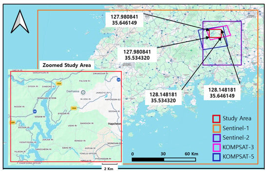
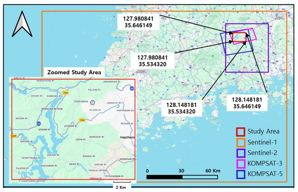
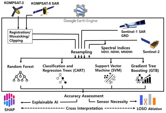
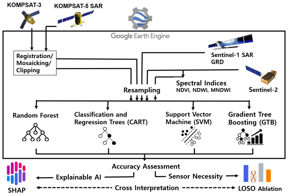
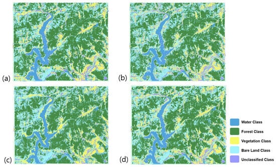
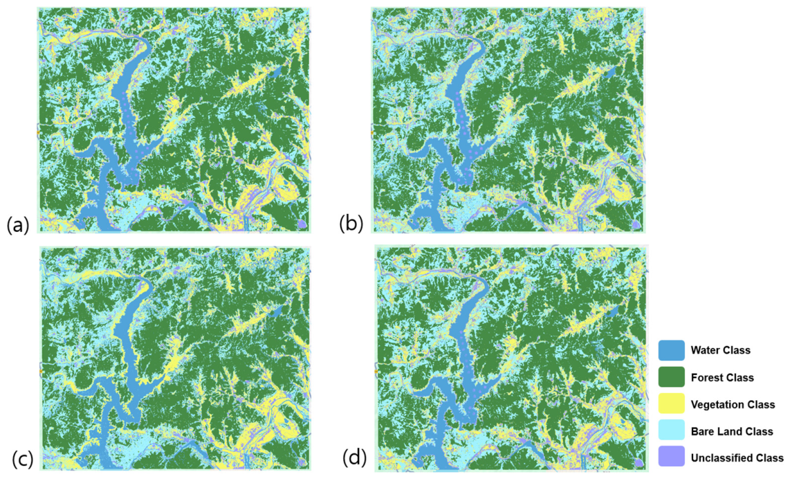
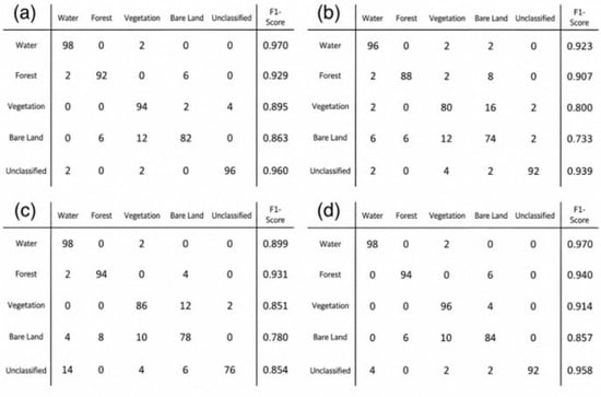
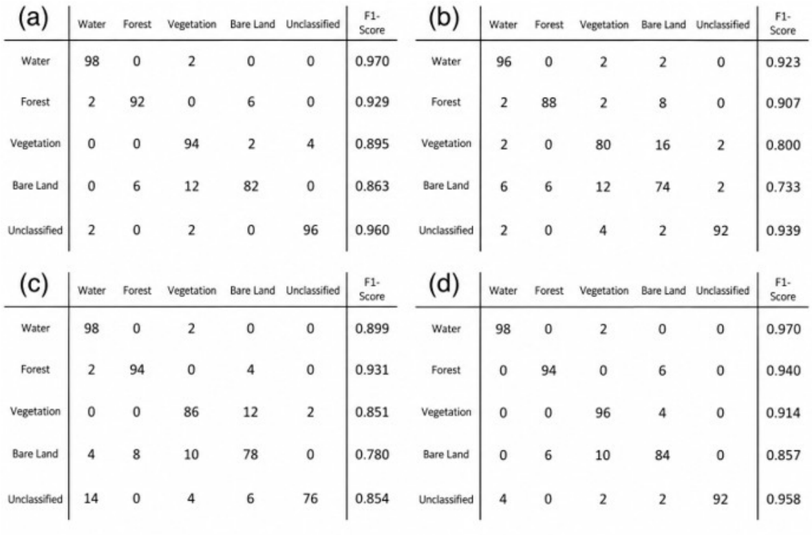
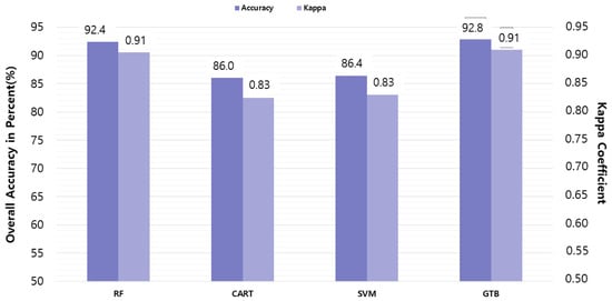
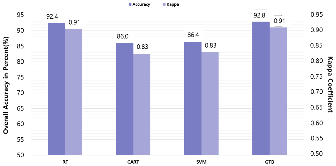
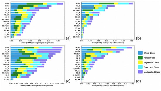
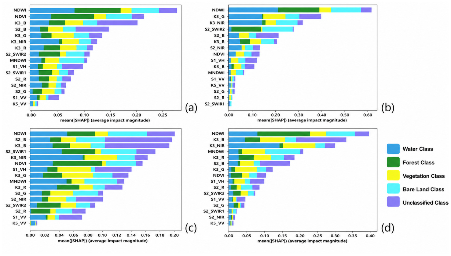
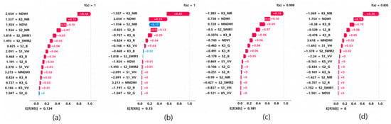
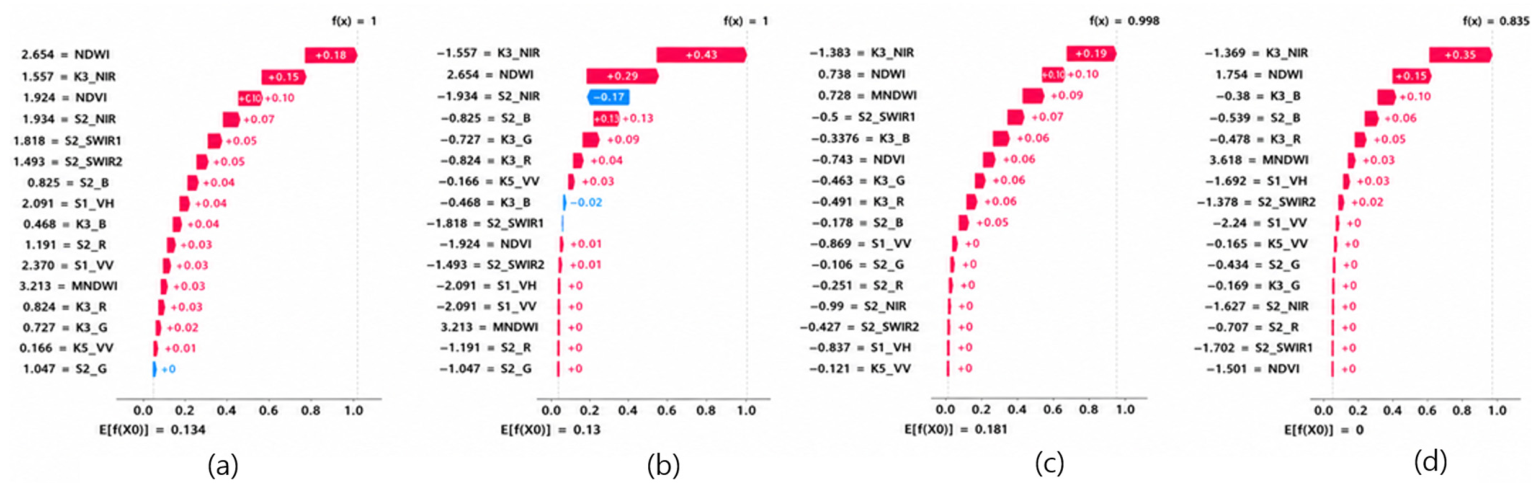
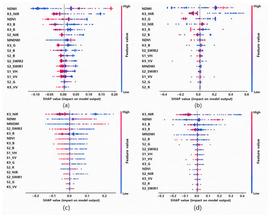
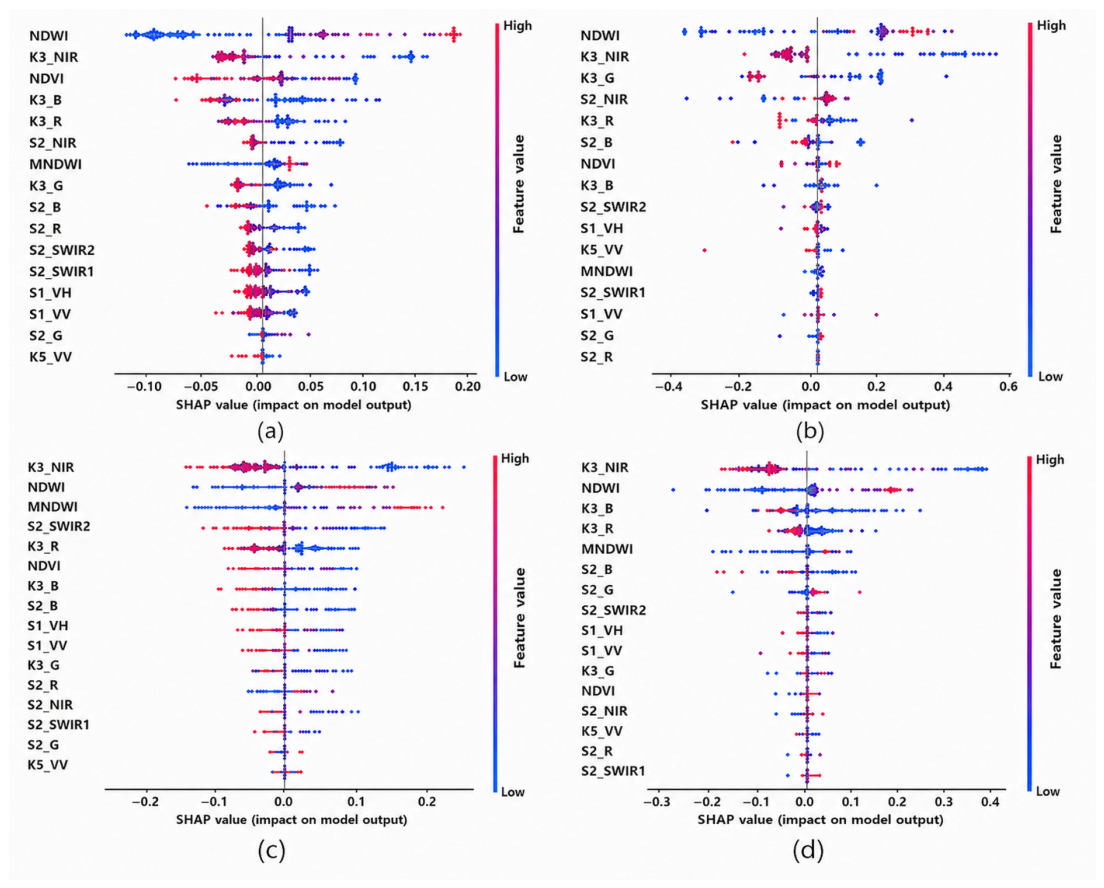
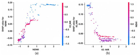
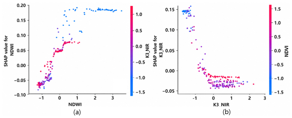
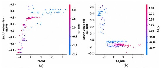
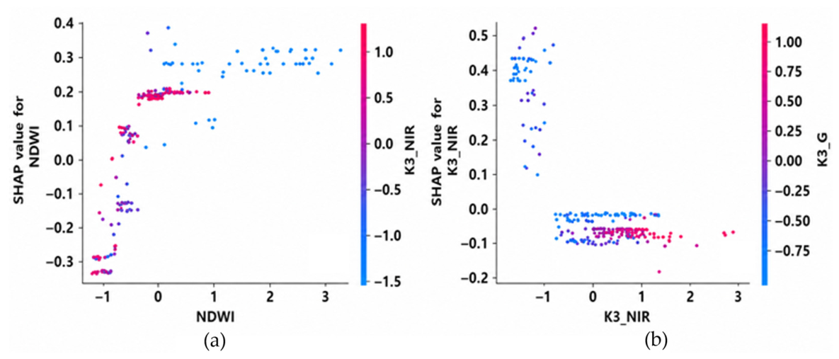
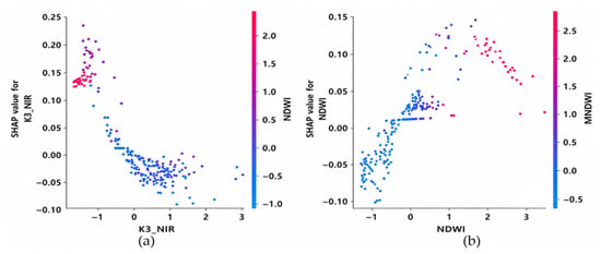
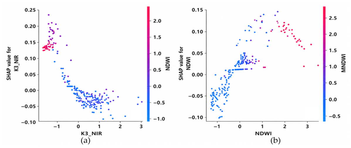
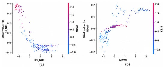
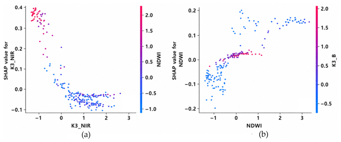
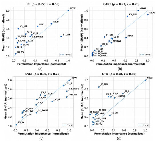
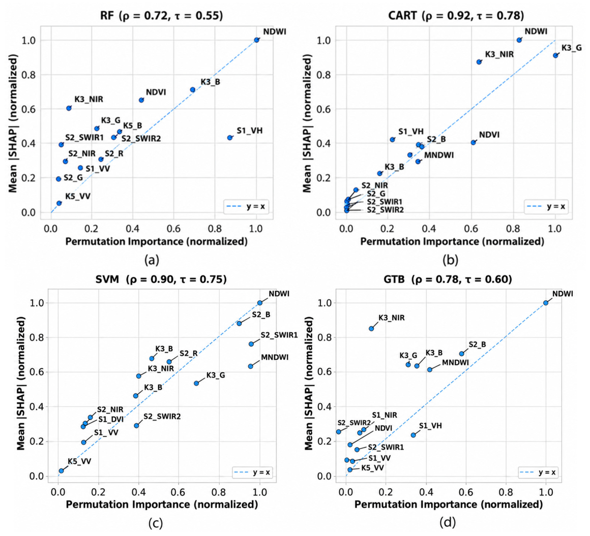
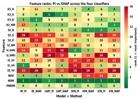
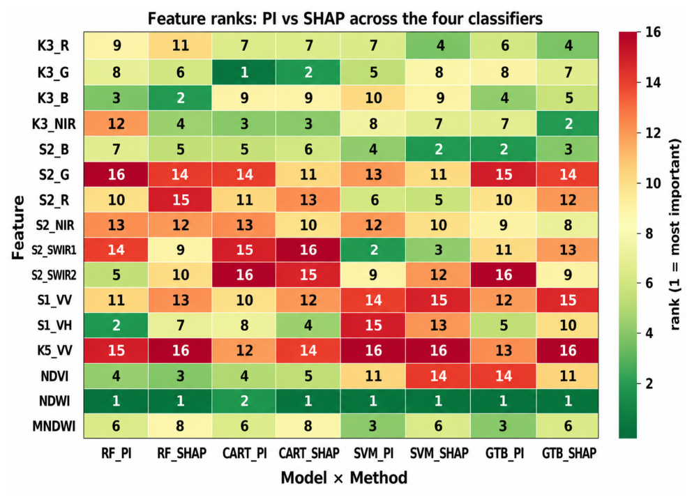
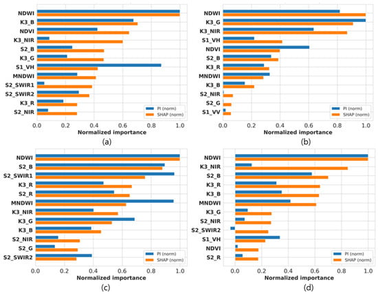
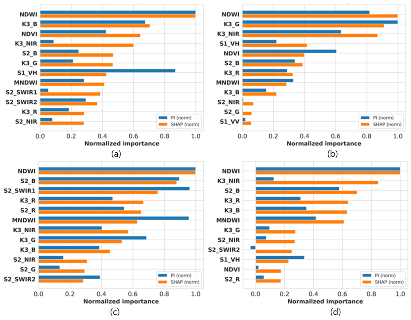
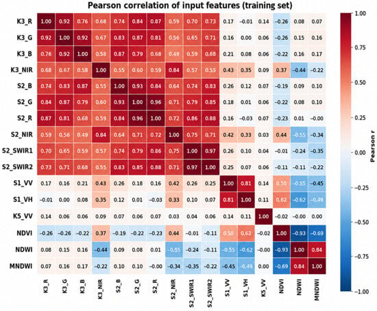
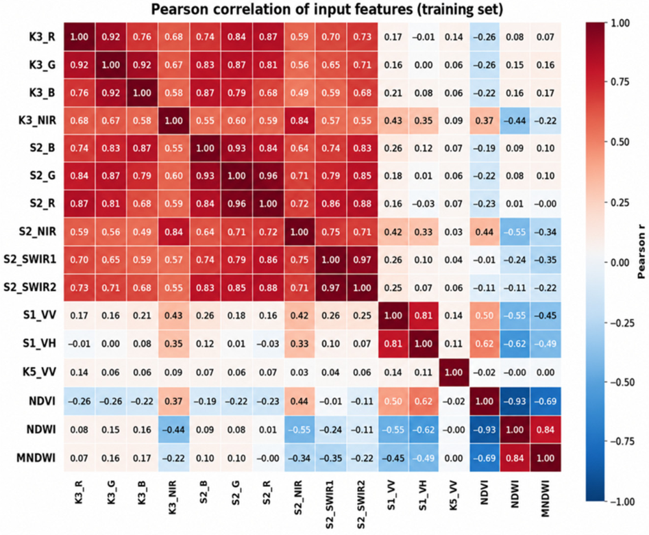
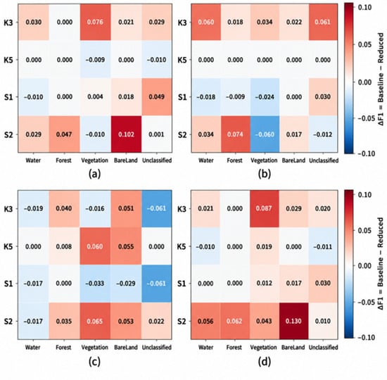
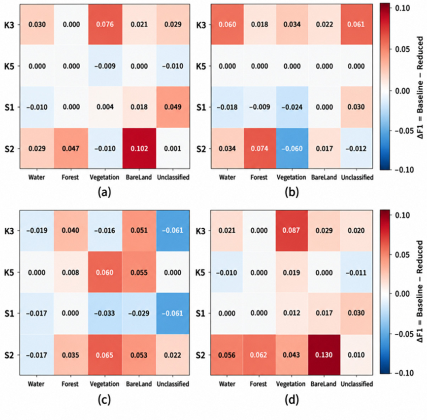

Disclaimer/Publisher’s Note: The statements, opinions and data contained in all publications are solely those of the individual author(s) and contributor(s) and not of MDPI and/or the editor(s). MDPI and/or the editor(s) disclaim responsibility for any injury to people or property resulting from any ideas, methods, instructions or products referred to in the content. |
© 2026 by the authors. Licensee MDPI, Basel, Switzerland. This article is an open access article distributed under the terms and conditions of the Creative Commons Attribution (CC BY) license.