


Highlights
What are the main findings?
- Downscaling land surface temperature from 30 m to 10 m revealed 4.7 times more within-area thermal variation and reduced median hot- and cold-spot size from 18,000 to 700 m2.
- Land-cover composition and heterogeneity explained 65.5% of the added thermal variation, with tree canopy showing the strongest association.
What are the implications of the main findings?
- Downscaling reveals meaningful fine-scale urban heat patterns that are obscured in conventional 30 m satellite products.
- Testing whether added thermal variation corresponds with independently mapped landscape features offers a practical evaluation method when high-resolution thermal observations are unavailable.
Abstract
Remotely sensed surface temperature data are widely used by researchers and municipal practitioners to characterize urban thermal patterns and assess the impacts of increasing urban heat. While satellite-derived land surface temperature (LST) data effectively identify broad-scale patterns, their 30 m spatial resolution limits their ability to resolve fine-scale thermal variability. Downscaling approaches have been developed to generate higher-resolution LST products; however, in the absence of independent, high-resolution surface temperature observations, it remains difficult to determine whether the additional spatial variation introduced by downscaling reflects meaningful landscape-related thermal structure or model-generated variability. Our objective was to evaluate whether the additional spatial variation introduced by downscaling LST from 30 to 10 m was statistically consistent with independently derived land cover composition and landscape compositional heterogeneity. Using an open-source random forest model, we downscaled Landsat 8/9 LST to 10 m resolution using Sentinel-2-derived predictors over a summer season in Kelowna, BC, Canada. We quantified the additional thermal variation introduced through downscaling and used Generalized Additive Models (GAMs) to relate this variation to high-resolution land cover characteristics summarized within 100 m grid cells. Land cover composition and landscape compositional heterogeneity together explained 65.5% of the additional variation introduced by downscaling. Added thermal variation was most strongly associated with canopy and impervious cover, two landscape characteristics consistently identified as major controls on urban land surface temperature. These findings suggest that the additional spatial variation introduced through downscaling is consistent with independently derived landscape structure known to influence urban thermal patterns. Rather than providing direct validation of downscaled temperatures, this analysis offers an indirect means of evaluating whether downscaled LST produces interpretable, landscape-consistent thermal variability that may be useful for urban analysis and planning.
1. Introduction
As extreme summertime heat increasingly challenges cities, researchers and practitioners are seeking robust methods to characterize spatial and temporal patterns of urban temperature. Satellite-derived land surface temperature (LST) provides a widely accessible, often cost-free, and spatially continuous dataset for assessing urban thermal patterns at broad scales, typically at 30 m resolution. Consequently, LST assessments have become foundational for municipal heat-mapping initiatives. However, as cities move beyond coarse assessments toward fine-scale decision-making, the limitations of conventional 30 m LST data become evident. At this resolution, fine-scale thermal heterogeneity is often masked, which constrains our ability to evaluate how heat is experienced in everyday urban environments at the scale of human exposure [1].
In response to limitations in resolving fine-scale urban thermal heterogeneity using accessible remote-sensing methods, researchers have developed methods for downscaling LST. Downscaling LST typically involves using higher-resolution spectral information, or derived indices that are correlated with LST, to predict and redistribute LST at a finer spatial resolution than that of the original thermal sensor [2]. Early downscaling methods primarily relied on vegetation indices, such as the Normalized Difference Vegetation Index (NDVI), as linear predictors of LST [3,4,5]. While effective in relatively homogeneous landscapes and at coarser spatial resolutions [6], these single-variable NDVI-based linear models have been shown to perform poorly in irrigated, moisture-variable, or structurally complex urban systems, where thermal responses are often non-linear and driven by many interacting landscape characteristics [7,8,9,10].
Despite advances in LST downscaling, relatively little work has examined downscaling to high resolutions (e.g., 10 m), due in part to the difficulty of evaluating high-resolution outputs. This challenge is particularly pronounced in complex urban environments, where high structural and thermal heterogeneity coincide with limited availability of independent, high-resolution temperature data [11]. In response, researchers have often relied on aggregation–disaggregation approaches to evaluation, in which fine-resolution predictions are aggregated back to the original coarse resolution for comparison [2,10,12,13]. However, because this approach evaluates the downscaling output against the original sensor, it does not assess whether newly introduced variation reflects underlying spatial structure or model artefacts. Onačillová et al. (2022) [14] partly addressed this limitation by comparing 10 m downscaled LST to six in situ surface temperature measurements, but the point-based nature of these observations limited their ability to capture spatially continuous patterns. Together, these studies highlight the need for alternative approaches to assessing the added value of high-resolution LST products.
In this context, one promising approach is to evaluate whether downscaled LST captures variation that is consistent with known physical drivers of urban thermal patterns. Land cover composition is a key determinant of fine-scale thermal variability in cities, as the physical properties of surface materials influence energy balance processes, including radiation absorption, heat storage, and moisture availability, thereby shaping local thermal conditions [15]. In addition to composition, landscape heterogeneity—the spatial arrangement and diversity of these surface elements—shapes biophysical processes, influencing the magnitude and distribution of surface temperature [16,17,18]. Across a range of urban contexts, vegetated and pervious surfaces are consistently associated with lower surface temperatures, while impervious surfaces are associated with higher surface temperatures [19,20,21,22].
Research has shown that in heterogeneous urban environments, conventional satellite-derived LST fails to capture fine-scale thermal patterns relevant to human experiences of heat [1,23,24]. Although satellite-derived LST should not be interpreted as a direct measure of pedestrian thermal exposure, recent work suggests that surface temperature measured at sufficiently fine spatial scales can provide valuable information about the thermal environments experienced by people [25,26]. Fine-scale thermal measurements better resolve localized differences among urban surfaces and therefore may complement human-focused thermal metrics by characterizing the spatial distribution of thermally distinct environments.
Building on this understanding, we hypothesized that if the additional spatial variation introduced through downscaling reflects meaningful landscape-driven thermal structure rather than model-generated variability, it should be greatest in landscapes characterized by fine-scale compositional heterogeneity and exhibit relationships with land cover that are consistent with established urban thermal processes. To test this hypothesis, we evaluated whether a 10 m, open-source LST downscaling approach introduces additional spatial variation that is statistically consistent with independently derived land cover composition and landscape compositional heterogeneity. Specifically, we asked the following questions: (1) How much additional spatial variation is introduced by downscaling from 30 to 10 m resolution, and how does it alter the spatial structure of urban hot and cold spots? (2) Is the additional variation introduced through downscaling statistically consistent with independently derived land cover composition and landscape compositional heterogeneity? (3) Do the observed relationships between additional thermal variation and landscape characteristics align with established understanding of urban thermal processes? By answering these questions, we aim to provide additional evidence for interpreting the thermal information introduced through LST downscaling and its potential value for urban climate research and planning.
2. Materials and Methods
2.1. Study Area
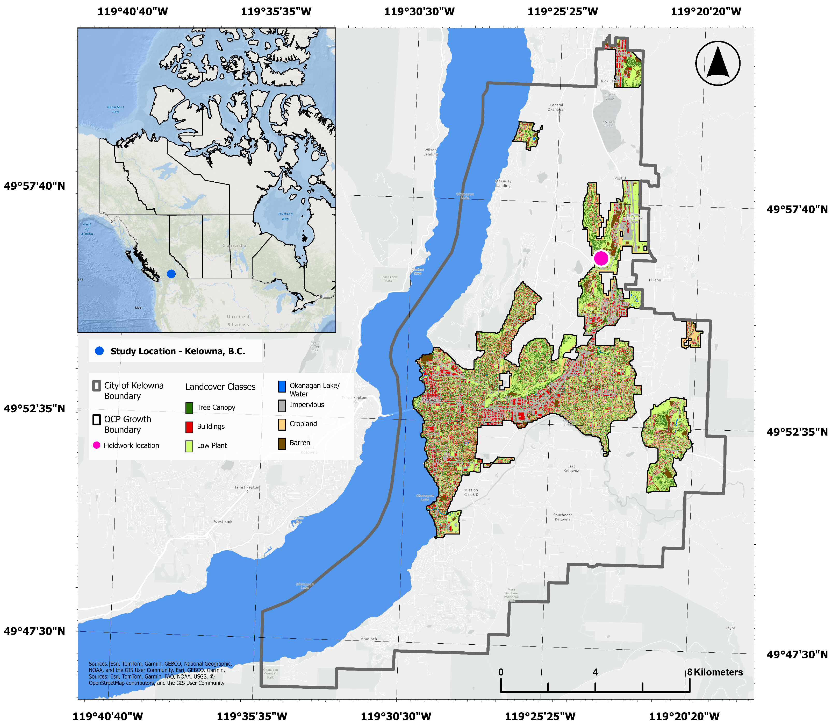
This research takes place in Kelowna, British Columbia (BC), Canada (CA). Kelowna is situated in the Okanagan Valley on the traditional, ancestral, unceded territory of the Indigenous Syilx/Okanagan people. To focus on urbanized zones within the City’s boundary, we constrained the study area by excluding areas identified as “Rural Lands” by the City’s Official Community Plan (OCP) ([27]; Figure 1).
Figure 1.
Context map of Kelowna, B.C, showing land cover classification within the study area, defined by the City’s Official Community Plan (OCP) Growth Boundary.
Kelowna is a fast-growing metropolis with roughly 170,000 residents and experiences a semi-arid climate. At 344 m above sea level, the city typically receives around 37 cm of annual precipitation and averages a summer daytime high temperature of 27 °C. The Okanagan Lake runs along the west side of Kelowna, spanning 100 km in length [28].
Kelowna provides an ideal setting for evaluating high-resolution LST products because its semi-arid environment creates pronounced fine-scale thermal contrasts driven by irrigation, vegetation, impervious surfaces, and proximity to water. These strong spatial gradients produce a highly heterogeneous urban landscape that is well suited for assessing whether downscaling captures meaningful thermal variation beyond that resolved by conventional 30 m satellite-derived LST. Furthermore, through our research partnership with the City of Kelowna, conventional 30 m LST products were found to be useful for identifying city-wide heat patterns but lacked the spatial detail needed to evaluate fine-scale management interventions such as planting prioritization and landscape design [29]. The city’s ongoing climate adaptation and urban forestry initiatives also provide a practical context in which higher-resolution thermal information may support urban planning decisions.
2.2. Explanatory Variables
2.2.1. Land Cover
We used a high-resolution (50 cm) 2023 land cover dataset with seven classes: tree canopy, buildings, low plant, water, impervious, cropland, and barren. The dataset was derived from 2023 LiDAR, 2023 four-band orthoimagery, 2023 tree canopy vectors, and 2021 building vectors using an object-oriented approach in eCognition Developer v10.4 (Trimble Geospatial, Westminster, CO, USA, 2025), following methods established by Jarlath O’Neil-Dunne and the University of Vermont Spatial Analysis Laboratory, and employed in numerous other studies [30,31,32]. An accuracy assessment was conducted using 500 points proportionally stratified across each land cover class based on their area, resulting in an overall accuracy of 94%.
2.2.2. Shannon Diversity Index
Landscape compositional heterogeneity was quantified using Shannon’s Diversity Index (SHDI), calculated within analysis units (see Section 2.5.1) using the PyLandStats tools (version 3.1.0) [33]. This index was selected to measure landscape compositional heterogeneity, capturing the number of classes present and the relative abundance of each class.
2.3. Landsat-Derived LST30
LST at 30 m resolution (hereafter LST30) was derived from the Thermal Infrared Sensor (band 10) aboard Landsat 8 and 9 (Level 2 product, ST_B10, wavelength = 10.60–11.19 μm). All available imagery between 1 June and 31 August 2023 was included, resulting in a total of 21 unique overpasses. The average daily maximum air temperatures for June were 25 °C, and 28 °C for July and August (Kelowna International Airport weather station data).
Cloud and atmospheric interference were removed from images using the Landsat QA_PIXEL bitmask, which is a band that indicates cloud coverage and other atmospheric conditions impacting pixel quality. Pixels flagged as dilated clouds (bit 1), high-confidence cirrus (bit 2), clouds (bit 3), and cloud shadows (bit 4) were excluded. Only pixels free of all four conditions were retained.
Surface temperature for each pixel was calculated using United States Geological Survey (USGS) corrective scaling factors [34]:
A mean composite was generated by averaging all cloud-free observations per pixel across the study period, producing a temporally stable representation of summer thermal conditions.
2.4. Downscaled LST10
LST was downscaled to 10 m resolution (hereafter LST10) using a random forest-based approach implemented in Google Earth Engine, adapted from the open-source workflow developed by Ramadhan (2024) [35]. We followed the general structure of this workflow while modifying predictor selection and preprocessing steps to better reflect the urban context of our study area.
2.4.1. Predictor Variable Processing
Sentinel-2 Level-2A imagery was used to derive predictor variables, also known as scaling factors. We tested 16 candidate predictors for significance with LST30. These predictors were based on Ramadhan (2024) [35], with two modifications: we included NDVI and removed digital elevation-derived variables (NASA SRTM; [36]). The final set of tested predictors comprised six Sentinel-2 bands, seven differential indices, and three Sentinel-2-based land cover derivatives. Together, these simple land cover variables represented wetness, greenness, and dryness (Table 1).
Table 1.
Compilation of variables tested for predicting land surface temperature downscaled to 10 m resolution (LST10), and their native resolutions.
We obtained 37 images between 1 June and 31 August 2023. Pixels contaminated by clouds, aerosols, or heavy haze were removed using the Cloud Score+ S2_HARMONIZED dataset, with a threshold of 0.6 applied to retain only high-quality observations [37]. Reflectance values were rescaled using a factor of .
For each remaining pixel, we generated mean composites to represent typical clear-sky conditions at 10 m resolution. Bands originally at 20 m resolution (e.g., short-wave infrared) were resampled to 10 m, meaning that their effective spatial detail is coarser than native 10 m bands.
2.4.2. Random Forest Model
An RF model was employed to predict LST10, as it is well-suited to capturing non-linear and multivariate relationships between LST and high-resolution urban surface characteristics [9,38,39,40]. To train the RF model, we adapted the workflow from Ramadhan (2024) [35] so that all Sentinel-2 predictors (Table 1) were aggregated to 30 m resolution to align with LST30 using an area-weighted mean reducer (reduceResolution) in Google Earth Engine (GEE; [38,41]).
Predictor selection followed a two-step process to identify variables that captured complementary information about surface properties while minimizing redundancy. Because all candidate predictors were selected based on their established relationships with land surface temperature in previous downscaling studies [40], our objective was not to identify an optimal predictor set but rather to retain a parsimonious set of variables representing distinct surface characteristics. First, the six variables most strongly correlated with LST were identified using Pearson’s correlation coefficient. Second, inter-variable collinearity was assessed using a Pearson correlation matrix, and the three variables with the lowest pairwise correlations were retained for the final model. Similar reductions in predictor number have been shown to maintain downscaling accuracy while reducing computational complexity [38].
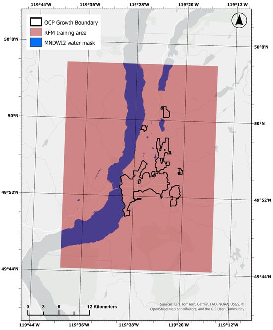
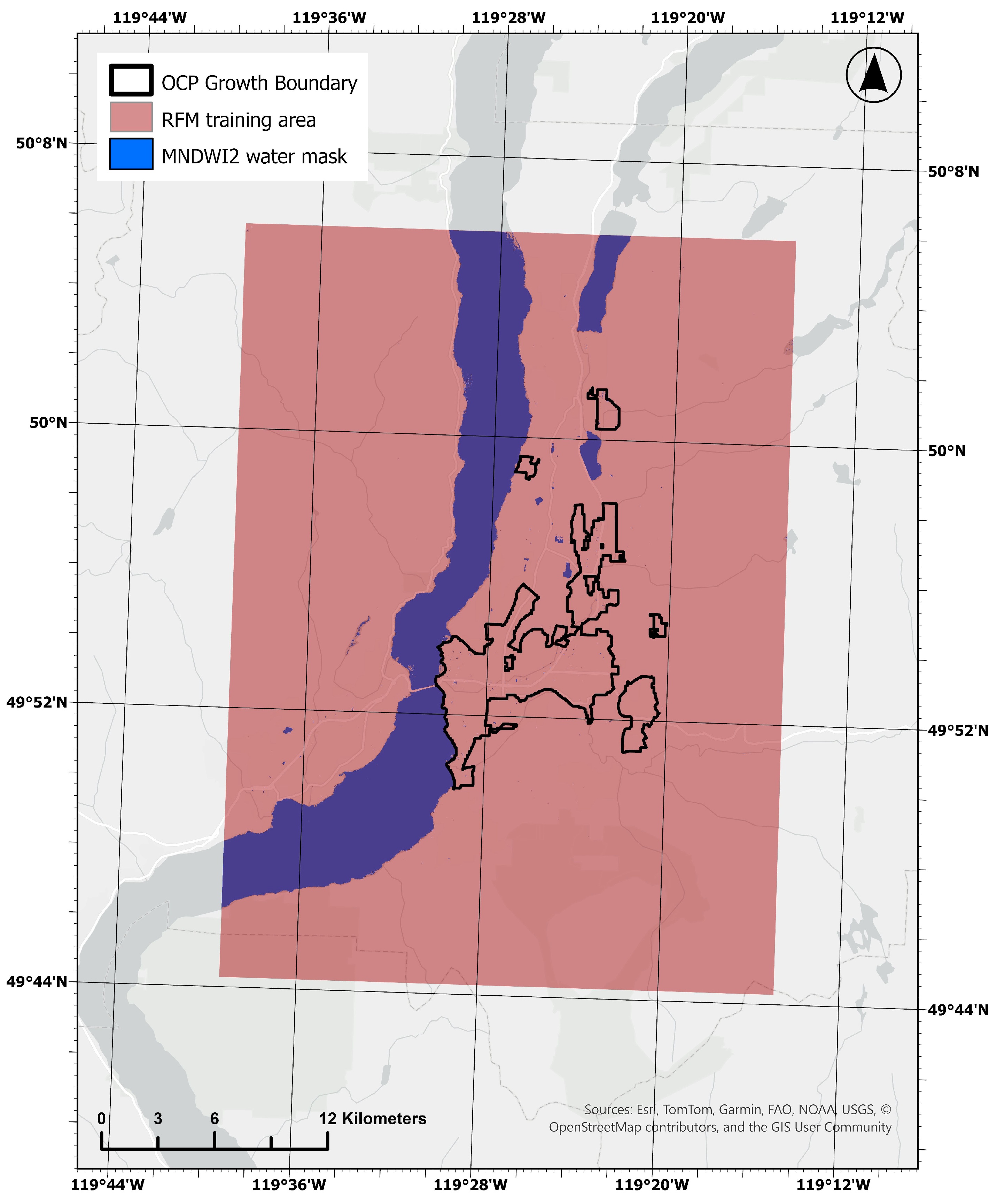
To train the RF model, we used an area extending beyond the primary study boundary to increase the number of sample points (Figure 2). We adapted the approach of Ramadhan (2024) [35] to exclude water bodies due to instability in thermal–spectral relationships, using a binary water mask from the Modified Normalized Difference Water Index (MNDWI2), with a threshold of >0.3. The RF model was implemented using the smileRandomForest algorithm in Google Earth Engine. A total of 2000 random samples were generated and partitioned into a 70/30 training and validation split. For the smileRandomForest model, we used the default seed value of 0 and set numberOfTrees to 50. The trained model was then applied to the 10 m Sentinel-2 grid to produce downscaled LST10 estimates.
Figure 2.
The extent of the RF model training area (red). Blue areas represent the water-masked pixels that were excluded from training data. The OCP Growth Boundary outline represents the study area.
Our training and validation split aligns with reported ratios in the RF-based LST downscaling literature. Njuki et al. (2020) [39] also used a 70/30 ratio, and Wang et al. (2020) [42] used a similar split of 60/40. Our numberOfTrees parameterization falls within the stable accuracy range identified by Wang et al. (2020) [42]. Further, James et al. (2023) [43] point out that the exact number of decision trees is less important, so long as the value is sufficiently large. Future studies could explore these parameters more thoroughly and perform sensitivity analyses to assess how parameterization influences downscaling accuracy.
2.5. Data Analysis
2.5.1. Question 1: Quantifying Added Thermal Variability and Spatial Clustering
To compare LST30 to LST10, summary statistics were calculated within a city-wide grid. Grid cell size was selected by evaluating sensitivity to the Modifiable Areal Unit Problem (MAUP), whereby spatial aggregation can influence analytical results [44,45]. For each grid resolution, we calculated the difference in standard deviation between LST10 and LST30:
Sensitivity of was assessed across grid cell sizes of 100, 200, 300, 400, and 500 m (Table A1). The distribution of was largely consistent across grid sizes, indicating that the response variable was relatively stable across the aggregation scales tested. Therefore, subsequent analyses were conducted at 100 m, the finest aggregation scale with stable results.
Spatial clustering of LST30 and LST10 was assessed using the Getis–Ord Gi* statistic [46], implemented via the Hot Spot Analysis tool in ArcGIS Pro (Version 3.6.3). Each LST raster was converted to point features, and spatial relationships were defined using a fixed distance band corresponding to the eight nearest neighboring cells. Distance thresholds of 44 m (LST30) and 15 m (LST10) were used to approximate this neighborhood structure following Queen’s contiguity. Statistical significance was evaluated at p < 0.05.
2.5.2. Questions 2 and 3: Developing a Generalized Additive Model (GAM)
Consistent with recent urban climate research [47,48,49,50], we developed a Generalized Additive Model (GAM) to capture non-linear relationships between biophysical explanatory variables and the thermal response variable. GAMs were selected over machine learning approaches, which may have higher predictive power, to retain mechanistic interpretability of functional relationships. All statistical analyses were performed in R (version 4.6.0) using the mgcv package (version 1.9.3) [51].
The GAM was used to explain the change in surface temperature variation between LST30 and LST10, quantified as (standard deviation of LST10—standard deviation of LST30). The key explanatory variables were four land cover classes—tree canopy, building, low plant, and impervious cover—as well as SHDI, representing both composition and compositional heterogeneity (Table 2). Water, cropland, and barren land cover classes were excluded due to low prevalence and minimal contribution within analysis units.
Table 2.
Summary of variables used in the Generalized Additive Models. Each variable was summarized within 100 m grid cells applied across the study area, except for latitude and longitude.
Predictor variables were modelled as one-dimensional smooth terms using penalized thin plate regression splines. To account for spatial trends and autocorrelation, we included a two-dimensional thin plate regression spline of UTM Easting and Northing as a covariate. Smoothness parameters were estimated using Restricted Maximum Likelihood (REML). Basis dimensions were set to k = 10 for land cover predictors to allow for moderate flexibility, and k = 150 for the spatial term to capture fine-scale spatial dependency.
Model structure and parameterization were evaluated through a series of sensitivity analyses. To assess the adequacy of the spatial smooth, we compared models with varying basis dimensions (k) and evaluated residual spatial autocorrelation using the spdep package (version 1.4.1) [52], with a 150 m distance-based neighborhood approximating Queen’s contiguity. The selected spatial basis dimension (k = 150) minimized residual spatial autocorrelation while retaining model flexibility. Predictor inclusion was evaluated using Akaike’s Information Criterion (AIC), comparing the global model to reduced models with individual predictors removed. In all cases, the global model yielded the lowest AIC (ΔAIC < 6; [53]), supporting retention of all predictors.
Given the high concurvity typical of urban ecological data [47,48,50], which limits interpretation of predictor effects in GAMs [54,55], we used the gam.hp package (version 0.0.5) [56] to assess the relative importance of predictor variables. This approach uses hierarchical partitioning to decompose explained deviance into relative individual contributions. These estimations of variable importance are independent of predictor order and reduce the effect of collinearity on interpretation, providing an unbiased estimate.
2.5.3. Supplementary Field Data Collection
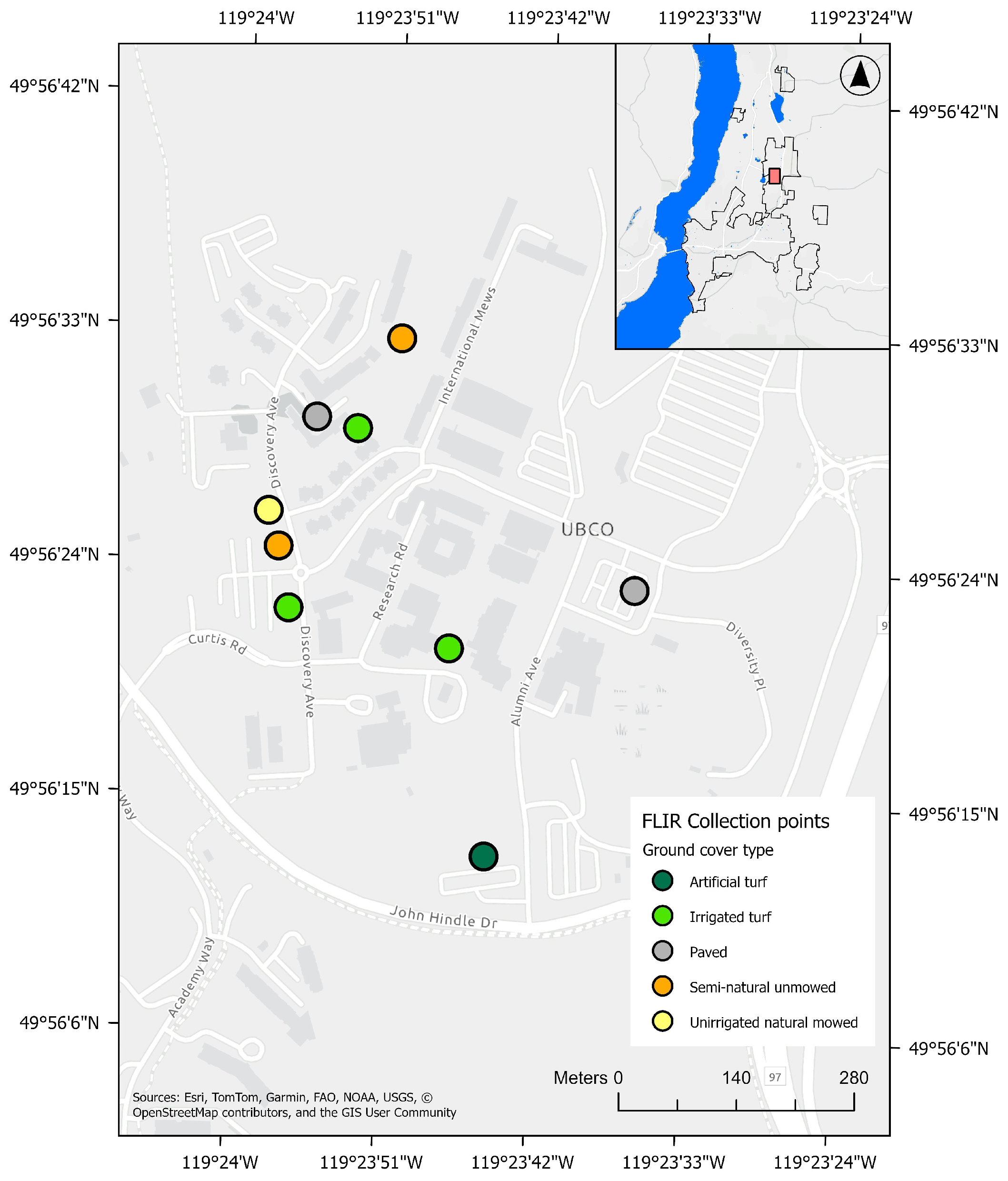
To provide an independent point of comparison with the downscaled LST product, we collected supplementary point-based surface temperature measurements on 22 June 2026 during the Landsat 9 overpass window (09:30–10:45 PDT). These observations were not intended as a formal validation of the downscaled LST product because of their limited spatial extent, but rather as a preliminary field-based comparison between satellite-derived and observed surface temperatures.
Sampling locations were selected to represent a range of common urban ground cover types found in Kelowna and represented within the LST10 product (Table 3). Building rooftops and tree canopies were excluded because they could not be measured directly from ground level. To maximize comparability with the satellite-derived LST, sampling was restricted to open, sunlit locations where a single ground cover type occupied the majority of the corresponding LST10 pixel.
Table 3.
Description of sampling points across five different ground cover types. Refer to Figure A1 for the location of each point.
Surface temperatures were measured using a handheld Forward Looking Infrared (FLIR) camera, the FLIR C5 compact camera (Teledyne Inc., Thousand Oaks, CA, USA). At each sampling location, four thermal images were collected from positions approximately 5 m from the sample point in each of the four cardinal directions. Surface temperature was extracted from the centre of each image, corresponding to the sampling location, and the four measurements were averaged to obtain a representative surface temperature for comparison with the satellite-derived LST.
To temporally align the field data with the LST images, we retrieved the Landsat 9 image from 22 June 2026 (using the same LST derivation methods described earlier, apart from the temporal compositing step) and performed the downscaling model on this single image.
3. Results
3.1. Land Cover Descriptive Statistics
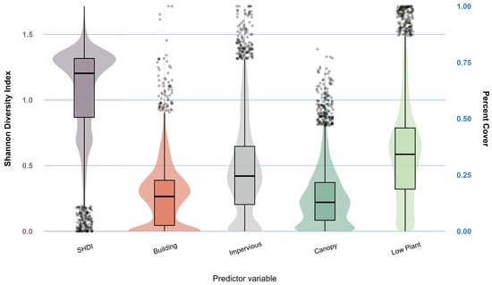
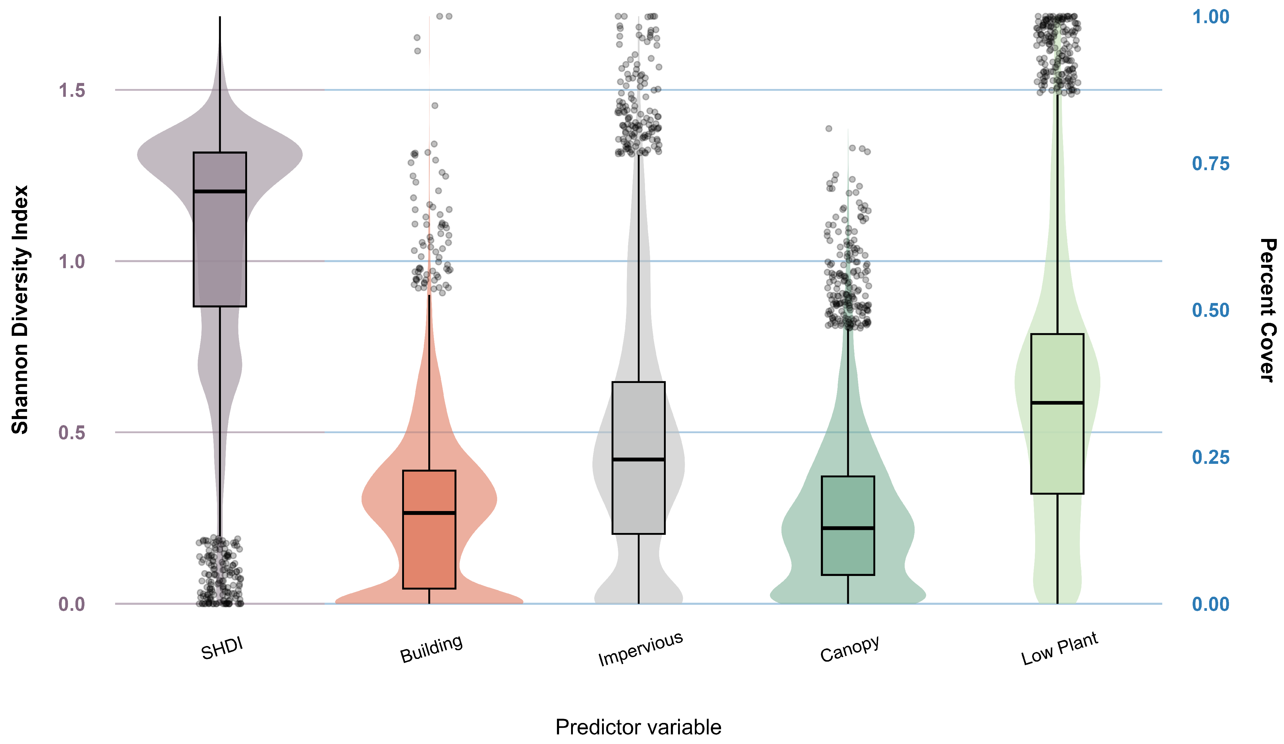
Across the 6069 100 m grid cells in the study area, the Shannon Diversity Index (SHDI) had a median of 1.20 (SD = 0.33), ranging from 0 to 1.72 (Figure 3). Median land cover values were 34.2% for low plant (SD = 21.9), 24.5% for impervious (SD = 20.7), 15.4% for building (SD = 13.1), and 15.0% for tree canopy (SD = 12.9). All four land cover classes spanned zero to 100% cover, except for canopy cover, which ranged from zero to 80.8%.
Figure 3.
Distribution of SHDI and percent land cover composition across the study area (n = 6069). The shaded violins represent the density distribution of the values. Boxes represent the interquartile range of values, and the solid horizontal line within each box indicates the median. Outliers are shown as individual points outside the whiskers. Note the dual y-axes: SHDI corresponds to the scale on the left axis, while the four land cover variables correspond to the percent cover scale on the right axis.
All land cover variables included a concentration of grid cells at 0% cover. Building and canopy cover were more tightly distributed around their median values, whereas impervious and low plant cover showed a more even spread across their ranges.
3.2. LST10 Downscaling Model Results
Out of all predictor variables tested for inclusion in the downscaling model, NBR2 ( = 0.64), Band 12 ( = 0.62), NBR ( = 0.61), NDVI ( = 0.59), dryness ( = 0.59), and greenness ( = 0.58) showed the strongest correlations with LST30. Following inter-variable redundancy testing, NDVI, dryness, and Band 12 were retained as downscaling predictors due to their slightly lower pairwise correlations. RF model outputs indicated relatively equal variable importance across the selected predictors, with NDVI contributing 35.0%, dryness 33.0%, and Band 12 32.1%. The RF test sample accuracy for the model yielded an of 0.75 and an RMSE of 3.35 °C.
The supplementary field comparison generally supported our interpretation that the downscaled LST product better captured fine-scale differences among urban surface types than the original 30 m product (Table 4 and Table 5). Across all sampled surface types except artificial turf, LST10 was more similar to the FLIR-derived surface temperatures than LST30. Artificial turf was the only surface for which the 30 m product more closely matched the field measurements. This may reflect the relatively uncommon spectral signature of artificial turf within the training data compared with the more common urban surface types used to develop the model.
Table 4.
Field data results from FLIR hand-held surface temperature measurements compared to 2023 remotely sensed surface temperature measurements.
Table 5.
Field data results from FLIR hand-held surface temperature measurements compared to 2026 remotely sensed surface temperature measurements.
The relative ranking of surface temperatures among ground cover types was also more consistent between the FLIR measurements and LST10 than between the FLIR measurements and LST30 (Table 4 and Table 5). The largest differences between the 30 m and 10 m products occurred over irrigated surfaces, where coarse-resolution pixels are most likely to average cool irrigated vegetation with warmer surrounding land covers. Although these supplementary observations were limited in spatial extent and were not intended as a formal validation of the downscaled product, they provide additional evidence that the 10 m product better represents relative thermal differences among common urban surface types than the original 30 m product.
3.3. Question 1: How Much Additional Surface Temperature Variation Is Revealed by Downscaling, and How Does Downscaling Alter the Spatial Extent of Hot and Cold Spots?
3.3.1. Magnitude of Additional Surface Temperature Variation
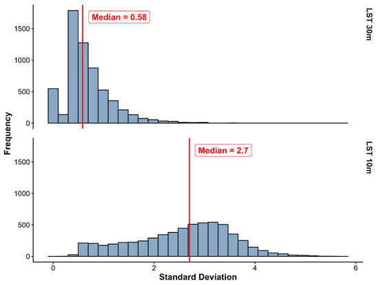
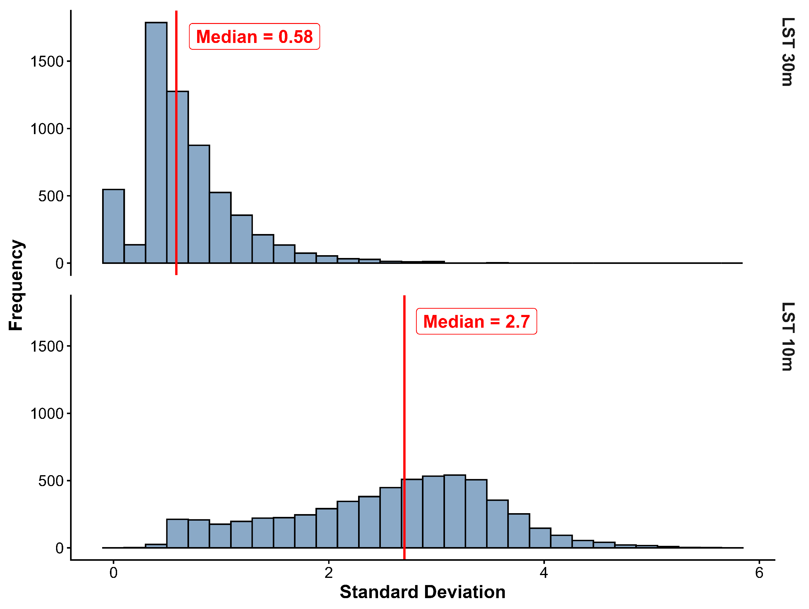
To quantify the surface temperature variation introduced by downscaling, we compared distributions of within-cell standard deviation in LST30 and LST10 across the 6069 100 m grid cells covering the city. Median within-cell variation increased 4.7-fold from LST30 to LST10 (Figure 4), indicating that downscaling reveals fine-scale thermal heterogeneity that is largely homogenized at 30 m resolution. LST30 exhibits a right-skewed distribution of standard deviation values, with most grid cells showing relatively low internal variability and only a small subset exhibiting higher heterogeneity. In contrast, LST10 displays a more symmetric distribution, suggesting that fine-scale thermal variability is more consistently detected across the landscape.
Figure 4.
Histograms of standard deviation values of each LST dataset within 100 m grid cells (n = 6069 for each histogram). The standard deviation of LST30 is on top, and the standard deviation of LST10 is on the bottom. The red line represents the median standard deviation of each dataset.
3.3.2. Changes in the Spatial Extent of Hot and Cold Spots
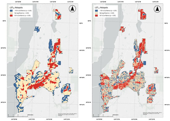
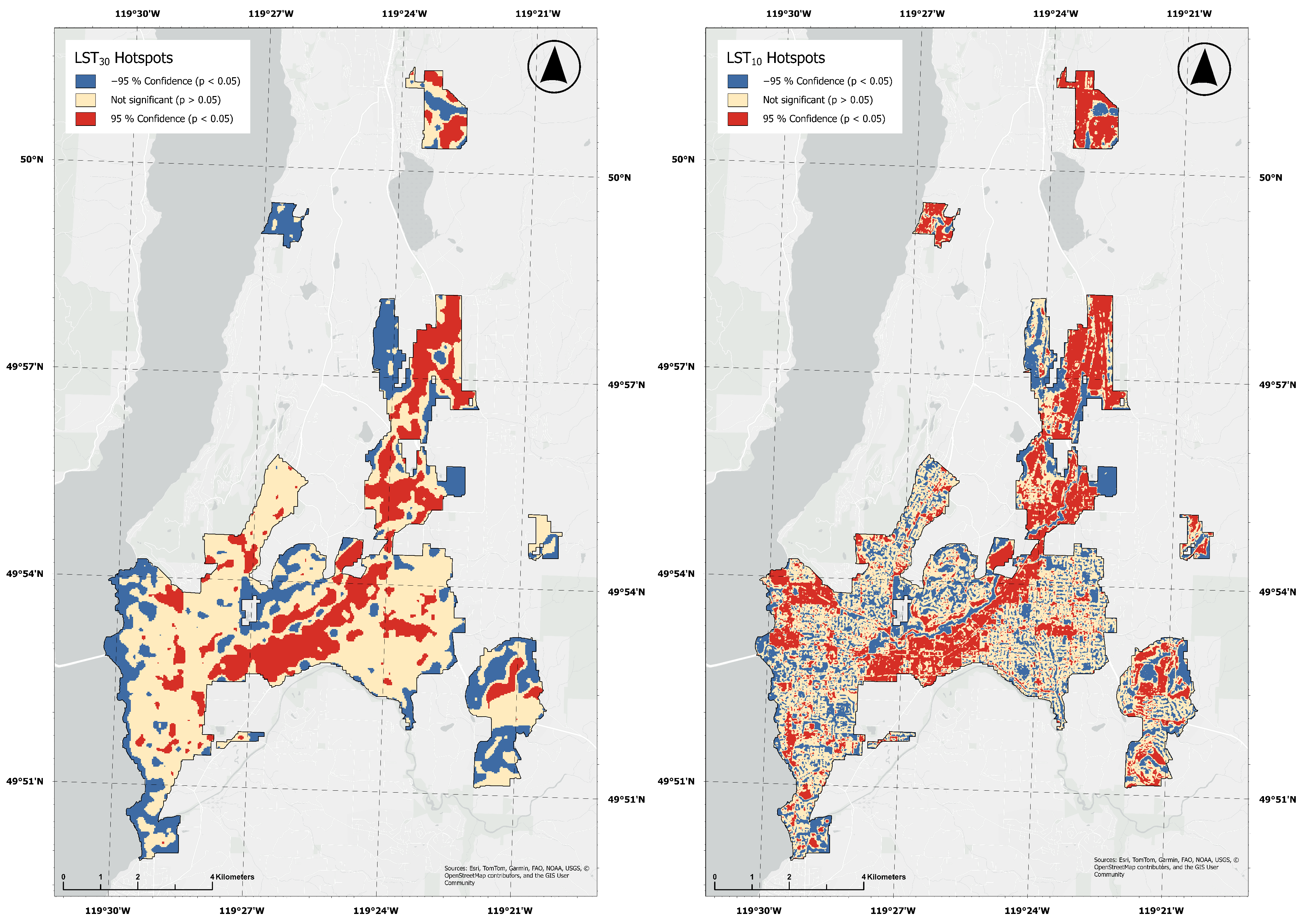
We assessed spatial clustering in LST30 and LST10 using the Getis-Ord Gi* statistic, comparing hot and cold spot detection at each dataset’s native spatial resolution (Figure 5). Downscaling reduced the spatial extent of significant (95% confidence; p value < 0.05) hot and cold clusters; median cluster size declined by a factor of 25.7, from 18,000 m2 (LST30) to 700 m2 (LST10).
Figure 5.
Land surface temperature hotspots (from the Getis-Ord Gi* statistic). Red and blue areas represent 95% confidence hot (red) or cold (blue) spots. The beige areas represent places with no significant clustering (p-value > 0.05).
A differential analysis of cluster classifications revealed that LST10 identified substantial new areas of statistically significant clustering. Specifically, 41.4% of locations classified as non-significant in LST30 exhibited significant hot or cold clustering in LST10. Of these newly detected clusters, 20.3 percentage points were hotspots and 21.1 percentage points were coldspots, whereas only 7.5% of locations previously identified as LST30 hot spots exhibited exhibited a ‘flipping’ pattern, in which the thermal direction of clustering reversed between methods (e.g., hot to cold or vice versa). In total, newly detected clusters in LST10 accounted for 26.9% of the total study site, whereas flipped clusters represented only 3.4% of the total study site. This indicates that downscaling primarily reveals previously masked fine-scale thermal structure in areas with mixed thermal signals rather than overturning thermal patterns identified in the original LST30 product.
3.4. Question 2: Do Land Cover Characteristics Explain the Additional Surface Temperature Variation Revealed from Downscaling?
To examine the factors associated with changes in thermal variability from LST30 to LST10, we modelled , representing the increase in within-cell thermal variability following downscaling, as a function of land cover composition and landscape compositional heterogeneity using a GAM. The GAM explained 65.5% of the variation in (adjusted = 0.65), and all explanatory variables were significantly associated with additional thermal variation (p < 0.001; Table 6). Based on F-values and hierarchical partitioning, canopy cover showed the strongest association with , exhibiting both the largest F-value and the greatest individual contribution to the explained variation.
Table 6.
Summary of results from the GAM and hierarchical partitioning. For the GAM results, concurvity (reported as the ‘observed’ value) represents collinearity of variables, and edf represents the degree of non-linearity (where 1 denotes linearity, and higher values indicate increasing complexity). For hierarchical partitioning, unique represents the deviance explained exclusively by the predictor, shared represents deviance attributed to collinearity, and partial D2 indicates relative importance as a percentage of the total deviance explained by the model (total model deviance = 65.5%).
SHDI, representing landscape compositional heterogeneity, was also significantly associated with (p < 0.001; Table 6), although its F-value was lower than that of several land cover variables. Because SHDI is derived from the same underlying land cover composition, it should not be interpreted as an independent effect but rather as a complementary measure of landscape heterogeneity. Interestingly, hierarchical partitioning attributed more explained variation to SHDI than to any individual land cover class except canopy cover, indicating that landscape compositional heterogeneity contributed information beyond that captured by any single land cover variable. Collectively, however, the land cover composition variables accounted for a greater proportion of the explained variation (59.0%) than SHDI alone.
3.5. Question 3: Do Relationships Between Land Cover and Added Temperature Variation Align with Established Theoretical Expectations?
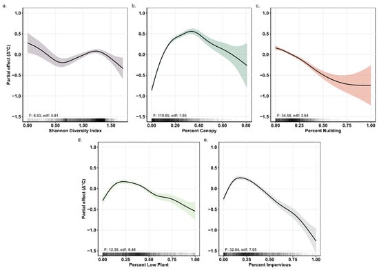
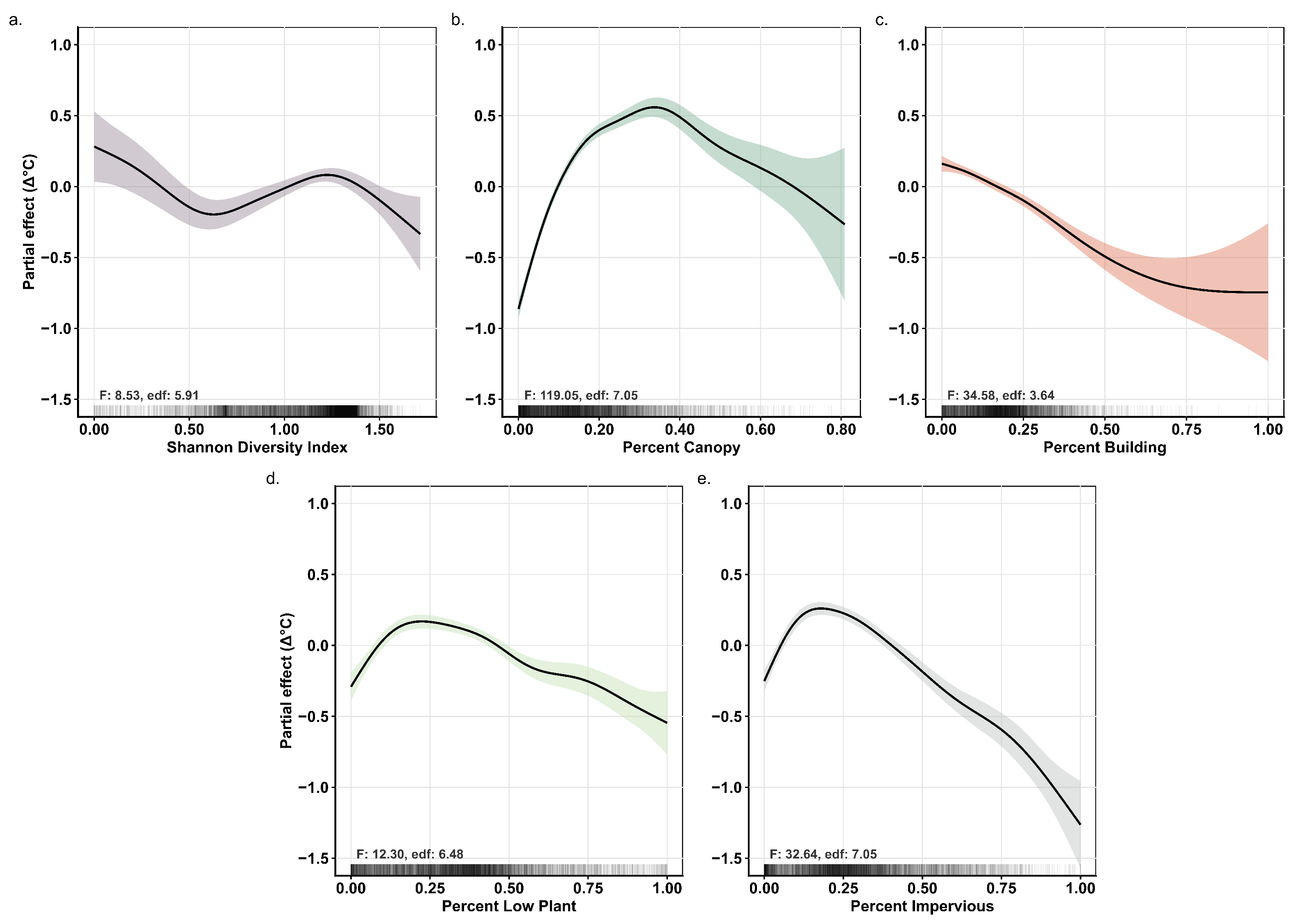
To better understand how the relationships between land cover characteristics and varied across the range of each explanatory variable, we examined the GAM smooth functions (Figure 6). Because the smooth functions represent partial effects while holding the remaining predictors constant, they should be interpreted as conditional statistical relationships rather than independent causal effects. The mean increase in within-cell thermal variation following downscaling () was 1.87 °C.
Figure 6.
Estimated smooth curves from the GAM, demonstrating the estimated partial relationships between predictor variables and added land surface temperature variation at a 100 m scale. The y-axis values represent the partial effect on variation, which is centred on zero, such that values above and below zero represent increases and decreases relative to the modelled mean (1.87 °C). A positive slope indicates increasing variation, and a negative slope indicates decreasing variation. The x-axis values represent the respective land cover percentages or land cover diversity (SHDI) within 100 m grid cells. Solid black lines represent the mean partial effect of each predictor, while shaded regions around the lines represent the 95% confidence intervals. The ‘rug’ marks along the x-axis depict a relative measure of data density. F-values (F) and effective degrees of freedom (edf) are reported for each term. (a) The conditional relationship between SHDI and ; (b) the conditional relationship between percent canopy cover and ; (c) the conditional relationship between percent building cover and ; (d) the conditional relationship between percent low plant cover and ; (e) the conditional relationship between percent impervious cover and .
Canopy cover and impervious cover exhibited the strongest and most clearly defined relationships with (Figure 6). increased rapidly with canopy cover between approximately 0 and 40% before gradually declining as canopy cover approached 100%. Impervious cover showed the opposite pattern, with decreasing as impervious cover increased. Low plant cover exhibited a similar non-linear relationship, with peaking at approximately 20% cover before gradually declining. Building cover was negatively associated with , indicating smaller differences between LST30 and LST10 in areas with greater building cover.
To examine the relationship between landscape compositional heterogeneity and additional thermal variation, SHDI was included alongside the land cover composition variables. increased slightly at intermediate SHDI values (approximately 0.6–1.3) but declined at both lower and higher values, indicating a non-linear relationship (Figure 6). Confidence intervals widened at higher SHDI values, reflecting fewer observations. Because SHDI is derived from the same underlying land cover composition as the explanatory variables, it should be interpreted as a complementary measure of landscape compositional heterogeneity rather than an independent effect.
Overall, the observed relationships indicate that the additional spatial variation introduced through downscaling was most strongly associated with landscape characteristics known to structure urban thermal environments, particularly canopy and impervious cover.
4. Discussion
4.1. Downscaling Reveals Meaningful Fine-Scale Thermal Heterogeneity
Downscaling from LST30 to LST10 revealed substantial fine-scale thermal variation that was not resolved in the conventional Landsat-derived product. At a 30 m resolution, individual pixels often contain multiple land cover types, averaging thermal conditions across heterogeneous urban landscapes and masking localized temperature differences [24,57]. By redistributing surface temperatures using high-resolution spectral information, the downscaled product revealed smaller, more spatially discrete thermal features that were not evident in the original imagery.
The reduction in hotspot size following downscaling illustrates this increased spatial detail. Rather than simply subdividing the original Landsat pixels, LST10 resolved localized thermal features that were previously aggregated within larger 30 m pixels. These finer-scale patterns more closely correspond to the scale at which urban landscapes are experienced and managed, including the scale of street trees, individual buildings, parks, and neighborhood planting interventions [1,23,25,26].
Although this study was not designed as a formal validation of the downscaled temperatures, our supplementary FLIR measurements provided an independent point of comparison that supported this interpretation. Across nearly all sampled surface types, LST10 more closely approximated field-measured surface temperatures than LST30, and better preserved the relative ranking of thermal conditions among common urban ground covers (Table 4 and Table 5). While these field observations were spatially limited and collected only within a small portion of the study area, they provide supplementary evidence that the downscaled product better represents fine-scale thermal differences than the original 30 m imagery.
Perhaps more importantly, the additional variation introduced through downscaling was strongly associated with independently derived land cover characteristics. Collectively, land cover composition and landscape compositional heterogeneity explained 65.5% of the variation in , indicating that the newly resolved thermal patterns were not randomly distributed across the landscape but were statistically consistent with known characteristics of urban form. Although this approach does not constitute direct validation of the downscaled temperatures, it provides evidence that the additional spatial variation introduced through downscaling is landscape-consistent and therefore likely represents meaningful thermal information rather than arbitrary model output.
4.2. Mixed Urban Landscapes Benefit the Most from Downscaling
The relationships observed between and land cover suggest that the greatest benefit of downscaling occurs in heterogeneous urban landscapes where contrasting surface types occur within the same 30 m Landsat pixel. Rather than increasing thermal variation uniformly across the city, downscaling introduced the greatest additional information where strong sub-pixel thermal contrasts were expected.
Canopy cover exhibited the strongest relationship with , with additional thermal variation increasing rapidly up to approximately 30–40% canopy cover before declining at higher canopy levels. A similar non-linear pattern was observed for low vegetation, while impervious cover showed the opposite trend, with additional thermal variation decreasing as impervious cover increased. Together, these relationships suggest that intermediate mixtures of vegetation and impervious surfaces contain the greatest unresolved thermal heterogeneity at Landsat resolution. In contrast, landscapes dominated by a single land cover type, such as highly impervious urban cores or extensively vegetated areas, are thermally more homogeneous, leaving less sub-pixel variability for downscaling to recover.
These patterns are consistent with established understanding of urban thermal processes. Numerous studies have identified canopy cover and impervious surfaces as the dominant controls on land surface temperature because they regulate radiation, evapotranspiration, and heat storage [19,58,59]. Our results extend this understanding by suggesting that these same landscape characteristics also determine where higher-resolution LST products provide the greatest additional information. In other words, downscaling appears to be most valuable in landscapes where coarse-resolution pixels contain mixtures of thermally contrasting surfaces.
One variable that was less influential than expected was low vegetation. We suspect this reflects the inability of the land cover classification to distinguish between irrigated and non-irrigated vegetation. In semi-arid cities such as Kelowna, differences in moisture availability strongly influence surface temperature [60,61,62] but are not explicitly represented in the land cover dataset. Consequently, areas classified simply as “low vegetation” may include cool irrigated lawns, dry grass, or exposed soil, all of which exhibit very different thermal behaviour. Future work incorporating irrigation or moisture information could help further explain this remaining variation.
4.3. Interpreting Landscape Compositional Heterogeneity
Landscape compositional heterogeneity, represented by SHDI, was significantly associated with but contributed less explanatory power than the land cover composition variables. This result is perhaps not surprising because SHDI summarizes the diversity of land cover types without describing the physical properties that directly influence surface temperature [63]. In contrast, variables such as canopy and impervious cover more directly represent processes governing radiation, moisture availability, and heat storage.
The non-linear relationship between SHDI and further suggests that thermal heterogeneity is not determined solely by the diversity of land cover classes. Moderate levels of compositional heterogeneity were associated with increased thermal variation, whereas both low and high SHDI values showed smaller increases in . This pattern indicates that landscapes containing many different land cover types are not necessarily thermally heterogeneous if those land covers have similar thermal properties. Conversely, relatively simple landscapes may exhibit substantial thermal variation when they contain strong contrasts between irrigated and non-irrigated surfaces or between vegetation and impervious materials.
Because SHDI is derived from the same underlying land cover composition variables included in the GAM, it should not be interpreted as an independent predictor of thermal variation. Instead, it serves as a complementary measure of overall landscape structure. Collectively, these findings suggest that the composition of urban landscapes provides greater explanatory power for additional thermal variation than diversity metrics alone, emphasizing the importance of considering both the types of land covers present and their thermal characteristics when evaluating fine-scale urban heat patterns.
4.4. Limitations and Future Directions
Despite the encouraging results, several limitations should be acknowledged. First, the random forest downscaling model is inherently difficult to interpret because the relationships between predictors and the final LST estimates are learned through a complex ensemble of decision trees rather than an explicit physical model [38]. While our objective was not to explain the internal mechanics of the random forest model, future work could investigate variable importance and feature selection using approaches such as recursive feature elimination [38] or SHAP analysis [64].
Second, our evaluation of the downscaled product remains indirect. Although the supplementary FLIR measurements provided an encouraging point of comparison, they were limited in spatial extent and were not intended as a comprehensive validation dataset. Similarly, the reported and RMSE values should be interpreted cautiously because they were derived using a conventional 70/30 random train-test split, and nearby samples may be spatially autocorrelated. Consequently, these metrics likely represent optimistic estimates of predictive performance. Future studies should incorporate spatial cross-validation or block-based validation together with more extensive high-resolution thermal observations to provide a more rigorous assessment of downscaled LST accuracy.
A further limitation is that we did not apply a residual bias correction to the downscaled temperatures. Residual correction, originally proposed by Kustas et al. (2003) [4] and subsequently adopted by several LST downscaling studies [65,66,67], can improve agreement between the downscaled and original Landsat products while reducing prediction bias. Because our primary objective was to evaluate whether the additional spatial variation introduced through downscaling was statistically consistent with independently derived landscape characteristics, improving agreement with the original Landsat product was not the focus of this study. Nevertheless, future work should examine how residual correction influences both model accuracy and the spatial patterns of thermal variability introduced through downscaling.
Our predictor selection procedure also represents a deliberate balance between model simplicity and computational efficiency. Candidate variables were selected based on their established relationships with land surface temperature, and a simple correlation-based approach was used to retain a parsimonious set of complementary predictors. Although similar approaches have been successfully applied in previous LST downscaling studies [13,40], future research could evaluate whether more sophisticated feature selection techniques or larger predictor sets improve model performance without introducing unnecessary complexity.
Finally, one predictor used in the random forest model, Sentinel-2 Band 12 (SWIR), has a native spatial resolution of 20 m and was resampled to 10 m prior to analysis. Consequently, the raw SWIR band does not contain true 10 m spatial information, although spectral indices derived from Band 12 combine this information with native 10 m Sentinel-2 bands. While this resolution mismatch should be recognized when interpreting the model inputs, the consistency of the downscaled thermal patterns with independently derived land cover characteristics suggests that the model captured meaningful fine-scale thermal variability despite this limitation.
5. Conclusions
This study demonstrates that downscaling Landsat-derived land surface temperature (LST) from 30 m to 10 m resolution reveals substantial fine-scale thermal heterogeneity that is not resolved in conventional satellite products. Rather than directly validating the downscaled temperatures, we evaluated whether the additional spatial variation introduced through downscaling was statistically consistent with independently derived land cover composition and landscape compositional heterogeneity. The strong associations between and established controls on urban thermal structure, particularly canopy and impervious cover, suggest that the additional variation introduced through downscaling reflects meaningful landscape patterns rather than arbitrary model output. These findings indicate that downscaled LST provides a more informative representation of urban thermal environments for ecological research, urban planning, and climate adaptation.
The workflow presented here combines publicly available Landsat and Sentinel-2 imagery with an open-source modelling framework, providing an accessible approach for generating higher-resolution LST products. More broadly, we propose that evaluating the landscape consistency of downscaled thermal variability provides a useful complement to conventional accuracy assessments, offering researchers and practitioners an additional means of assessing whether downscaled LST captures meaningful fine-scale thermal information when independent high-resolution thermal observations are unavailable.
Author Contributions
Conceptualization, E.S. and M.R.M.; methodology, E.S. and A.B.; formal analysis, E.S. and A.B.; investigation, A.B. and T.W.; resources, M.R.M.; data curation, M.F. and T.W.; writing—original draft preparation, E.S. and A.B.; writing—review and editing, A.B., E.S. and M.R.M.; visualization, E.S.; supervision, M.R.M.; project administration, M.R.M.; funding acquisition, M.R.M. All authors have read and agreed to the published version of the manuscript.
Funding
This research was funded by a Natural Sciences and Engineering Research Council of Canada (NSERC) Discovery Grant GR026733 and a City of Kelowna grant on planting feasibility. E.S. was partially supported by an NSERC Undergraduate Student Research Award (USRA) and University of British Columbia (UBC) Work Learn funding.
Data Availability Statement
Open source script: https://code.earthengine.google.com/dc51900e7654e929d608985b8e915928 (accessed on 17 July 2026). Please contact M.R.M. if the land cover dataset is needed.
Acknowledgments
The authors wish to thank the City of Kelowna, particularly Jennifer Miles and Todd Cashin, for continuing to ground this research in practical municipal needs and questions. We thank Jarlath O’Neil-Dunne and the members of the University of Vermont Lab for providing the methodological foundation and resources for that analysis. We also gratefully acknowledge Peter Ibsen for his early analysis support, Yuhao Lu for assistance during the initial brainstorming phases, and Tijmen Witvliet for his guidance with the early statistical analyses and brainstorming. Finally, we thank the members of the Urban Ecology and Sustainability Lab, including Ben Nixon, Brandon Weigand, Alex Mock, Hoi Kay So, and Logan Steinharter, for their ongoing support and collaboration.
Conflicts of Interest
Author Mark Fillo was employed by the company Diamond Head Consulting. The remaining authors declare that the research was conducted in the absence of any commercial or financial relationships that could be construed as a potential conflict of interest.
Appendix A
To evaluate the sensitivity of our GAM response variable (), we tested how the variable responded to being summarized at different scales (Table A1). We calculated in the same manner for each grid cell size ( = Standard Deviation of LST10 − Standard Deviation of LST30). We tested the outcomes across the study site using grid cells ranging from 100 m to 500 m, at 100 m intervals.
Table A1.
Sensitivity analysis of across various grid cell scales.
In addition to our GAM analysis of satellite-derived LST variation, we collected supplementary field data. The locations of our FLIR measurements were all located within our study site (Figure A1). We sampled across five different distinct ground covers, to begin to form an independent point of comparison.
Figure A1.
FLIR image locations on 22 June 2026. Field data were collected on the University of British Columbia Okanagan (UBCO) Campus. We took unique measurements at nine points, across five ground cover types. Red box in map inset shows UBCO location relative to the greater study site boundary in black.
References
- Kelly Turner, V.; Rogers, M.L.; Zhang, Y.; Middel, A.; Schneider, F.A.; Ocón, J.P.; Seeley, M.; Dialesandro, J. More than surface temperature: Mitigating thermal exposure in hyper-local land system. J. Land Use Sci. 2022, 17, 79–99. [Google Scholar] [CrossRef] [Scilit]
- Zhan, W.; Chen, Y.; Zhou, J.; Wang, J.; Liu, W.; Voogt, J.; Zhu, X.; Quan, J.; Li, J. Disaggregation of remotely sensed land surface temperature: Literature survey, taxonomy, issues, and caveats. Remote Sens. Environ. 2013, 131, 119–139. [Google Scholar] [CrossRef] [Scilit]
- Sandholt, I.; Rasmussen, K.; Andersen, J. A simple interpretation of the surface temperature/vegetation index space for assessment of surface moisture status. Remote Sens. Environ. 2002, 79, 213–224. [Google Scholar] [CrossRef] [Scilit]
- Kustas, W.P.; Norman, J.M.; Anderson, M.C.; French, A.N. Estimating subpixel surface temperatures and energy fluxes from the vegetation index–radiometric temperature relationship. Remote Sens. Environ. 2003, 85, 429–440. [Google Scholar] [CrossRef] [Scilit]
- Agam, N.; Kustas, W.P.; Anderson, M.C.; Li, F.; Neale, C.M. A vegetation index based technique for spatial sharpening of thermal imagery. Remote Sens. Environ. 2007, 107, 545–558. [Google Scholar] [CrossRef] [Scilit]
- Inamdar, A.K.; French, A. Disaggregation of GOES land surface temperatures using surface emissivity. Geophys. Res. Lett. 2009, 36, 2008GL036544. [Google Scholar] [CrossRef] [Scilit]
- Deng, C.; Wu, C. Examining the impacts of urban biophysical compositions on surface urban heat island: A spectral unmixing and thermal mixing approach. Remote Sens. Environ. 2013, 131, 262–274. [Google Scholar] [CrossRef] [Scilit]
- Ghosh, A.; Joshi, P. Hyperspectral imagery for disaggregation of land surface temperature with selected regression algorithms over different land use land cover scenes. ISPRS J. Photogramm. Remote Sens. 2014, 96, 76–93. [Google Scholar] [CrossRef] [Scilit]
- Li, W.; Ni, L.; Li, Z.L.; Duan, S.B.; Wu, H. Evaluation of Machine Learning Algorithms in Spatial Downscaling of MODIS Land Surface Temperature. IEEE J. Sel. Top. Appl. Earth Obs. Remote Sens. 2019, 12, 2299–2307. [Google Scholar] [CrossRef] [Scilit]
- Zawadzka, J.; Corstanje, R.; Harris, J.; Truckell, I. Downscaling Landsat-8 land surface temperature maps in diverse urban landscapes using multivariate adaptive regression splines and very high resolution auxiliary data. Int. J. Digit. Earth 2020, 13, 899–914. [Google Scholar] [CrossRef] [Scilit]
- Andriambololonaharisoamalala, R.; Helmholz, P.; Ivánová, I.; Jones, E.; Soon, S.; Bulatov, D.; Song, Y. Enhancing the spatial and temporal resolution of satellite-derived land surface temperature in urban environments: A systematic literature review. Urban Clim. 2025, 60, 102345. [Google Scholar] [CrossRef] [Scilit]
- Gao, L.; Zhan, W.; Huang, F.; Quan, J.; Lu, X.; Wang, F.; Ju, W.; Zhou, J. Localization or Globalization? Determination of the Optimal Regression Window for Disaggregation of Land Surface Temperature. IEEE Trans. Geosci. Remote Sens. 2017, 55, 477–490. [Google Scholar] [CrossRef]
- Xu, S.; Zhao, Q.; Yin, K.; He, G.; Zhang, Z.; Wang, G.; Wen, M.; Zhang, N. Spatial Downscaling of Land Surface Temperature Based on a Multi-Factor Geographically Weighted Machine Learning Model. Remote Sens. 2021, 13, 1186. [Google Scholar] [CrossRef] [Scilit]
- Onačillová, K.; Gallay, M.; Paluba, D.; Péliová, A.; Tokarčík, O.; Laubertová, D. Combining Landsat 8 and Sentinel-2 Data in Google Earth Engine to Derive Higher Resolution Land Surface Temperature Maps in Urban Environment. Remote Sens. 2022, 14, 4076. [Google Scholar] [CrossRef] [Scilit]
- Voogt, J.; Oke, T. Thermal remote sensing of urban climates. Remote Sens. Environ. 2003, 86, 370–384. [Google Scholar] [CrossRef] [Scilit]
- Cadenasso, M.L.; Pickett, S.T.A.; Schwarz, K. Spatial heterogeneity in urban ecosystems: Reconceptualizing land cover and a framework for classification. Front. Ecol. Environ. 2007, 5, 80–88. [Google Scholar] [CrossRef] [Scilit]
- Pickett, S.T.A.; Cadenasso, M.L.; Rosi-Marshall, E.J.; Belt, K.T.; Groffman, P.M.; Grove, J.M.; Irwin, E.G.; Kaushal, S.S.; LaDeau, S.L.; Nilon, C.H.; et al. Dynamic heterogeneity: A framework to promote ecological integration and hypothesis generation in urban systems. Urban Ecosyst. 2017, 20, 1–14. [Google Scholar] [CrossRef] [Scilit]
- Jung, M.C.; Dyson, K.; Alberti, M. Urban Landscape Heterogeneity Influences the Relationship between Tree Canopy and Land Surface Temperature. Urban For. Urban Green. 2021, 57, 126930. [Google Scholar] [CrossRef] [Scilit]
- Myint, S.W.; Wentz, E.A.; Brazel, A.J.; Quattrochi, D.A. The impact of distinct anthropogenic and vegetation features on urban warming. Landsc. Ecol. 2013, 28, 959–978. [Google Scholar] [CrossRef] [Scilit]
- Myint, S.W.; Zheng, B.; Talen, E.; Fan, C.; Kaplan, S.; Middel, A.; Smith, M.; Huang, H.p.; Brazel, A. Does the spatial arrangement of urban landscape matter? examples of urban warming and cooling in phoenix and las vegas. Ecosyst. Health Sustain. 2015, 1, 11878989. [Google Scholar] [CrossRef] [Scilit]
- Wetherley, E.B.; McFadden, J.P.; Roberts, D.A. Megacity-scale analysis of urban vegetation temperatures. Remote Sens. Environ. 2018, 213, 18–33. [Google Scholar] [CrossRef] [Scilit]
- Osborne, P.E.; Alvares-Sanches, T. Quantifying how landscape composition and configuration affect urban land surface temperatures using machine learning and neutral landscapes. Comput. Environ. Urban Syst. 2019, 76, 80–90. [Google Scholar] [CrossRef] [Scilit]
- Vanos, J.K.; Middel, A.; McKercher, G.R.; Kuras, E.R.; Ruddell, B.L. Hot playgrounds and children’s health: A multiscale analysis of surface temperatures in Arizona, USA. Landsc. Urban Plan. 2016, 146, 29–42. [Google Scholar] [CrossRef] [Scilit]
- Naserikia, M.; Hart, M.A.; Nazarian, N.; Bechtel, B.; Lipson, M.; Nice, K.A. Land surface and air temperature dynamics: The role of urban form and seasonality. Sci. Total Environ. 2023, 905, 167306. [Google Scholar] [CrossRef] [Scilit] [PubMed]
- Steinharter, L.; Ibsen, P.C.; deSouza, P.; McHale, M.R. The Surface Is Not Superficial: Utilizing Hyper-Local Thermal Photogrammetry for Pedestrian Thermal Comfort Inquiry. Remote Sens. 2026, 18, 348. [Google Scholar] [CrossRef] [Scilit]
- Ibsen, P.C.; McHale, M.R.; deSouza, P.N.; Steinharter, L.; Green, C., Jr.; Diffendorfer, J.E.; Warziniack, T. Moving toward a more human-oriented analysis of urban heat: Examining differences of heat exposure intensity at busy commuting locations. Environ. Res. Health 2026, 4, 015016. [Google Scholar] [CrossRef] [Scilit]
- City of Kelowna. 2040 Official Community Plan. 2022. Last Updated: 10 January 2022. Available online: https://www.kelowna.ca/our-community/planning-projects/2040-official-community-plan (accessed on 16 April 2026).
- City of Kelowna. City Profile. Available online: https://www.kelowna.ca/our-community/about-kelowna/city-profile (accessed on 16 April 2026).
- Miles, J. (City of Kelowna, Kelowna, BC, Canada). Personal communication, 2025.
- Zhou, W.; Troy, A. An object-oriented approach for analysing and characterizing urban landscape at the parcel level. Int. J. Remote Sens. 2008, 29, 3119–3135. [Google Scholar] [CrossRef] [Scilit]
- Beck, S.M.; McHale, M.R.; Hess, G.R. Beyond Impervious: Urban Land-Cover Pattern Variation and Implications for Watershed Management. Environ. Manag. 2016, 58, 15–30. [Google Scholar] [CrossRef] [Scilit] [PubMed]
- Rasmussen, S.; Warziniack, T.; Neel, A.; O’Neil-Dunne, J.; McHale, M. When Small Is Not Beautiful: The Unexpected Impacts of Trees and Parcel Size on Metered Water-Use in a Semi-Arid City. Remote Sens. 2021, 13, 998. [Google Scholar] [CrossRef] [Scilit]
- Bosch, M. PyLandStats: An open-source Pythonic library to compute landscape metrics. PLoS ONE 2019, 14, e0225734. [Google Scholar] [CrossRef] [Scilit] [PubMed]
- Saylor, K. Landsat 8-9 Collection 2 Level 2 Science Product Guide; U.S. Geological Survey: Reston, VA, USA, 2024.
- Ramadhan, R. An RF Approach to Downscaling Landsat LST Using Sentinel-2 [Source Code]. 2024. Available online: https://code.earthengine.google.com/ac986028b56a794aefd3ea54e9cb09ba (accessed on 16 April 2026).
- Farr, T.G.; Rosen, P.A.; Caro, E.; Crippen, R.; Duren, R.; Hensley, S.; Kobrick, M.; Paller, M.; Rodriguez, E.; Roth, L.; et al. The Shuttle Radar Topography Mission. Rev. Geophys. 2007, 45, 2005RG000183. [Google Scholar] [CrossRef] [Scilit]
- Pasquarella, V.J.; Brown, C.F.; Czerwinski, W.; Rucklidge, W.J. Comprehensive quality assessment of optical satellite imagery using weakly supervised video learning. In Proceedings of the 2023 IEEE/CVF Conference on Computer Vision and Pattern Recognition Workshops (CVPRW), Vancouver, BC, Canada, 17–24 June 2023; pp. 2125–2135. [Google Scholar] [CrossRef] [Scilit]
- Ebrahimy, H.; Azadbakht, M. Downscaling MODIS land surface temperature over a heterogeneous area: An investigation of machine learning techniques, feature selection, and impacts of mixed pixels. Comput. Geosci. 2019, 124, 93–102. [Google Scholar] [CrossRef] [Scilit]
- Njuki, S.M.; Mannaerts, C.M.; Su, Z. An Improved Approach for Downscaling Coarse-Resolution Thermal Data by Minimizing the Spatial Averaging Biases in Random Forest. Remote Sens. 2020, 12, 3507. [Google Scholar] [CrossRef] [Scilit]
- Pu, R.; Bonafoni, S. Thermal infrared remote sensing data downscaling investigations: An overview on current status and perspectives. Remote Sens. Appl. Soc. Environ. 2023, 29, 100921. [Google Scholar] [CrossRef] [Scilit]
- Agam, N.; Kustas, W.P.; Anderson, M.C.; Li, F.; Colaizzi, P.D. Utility of thermal image sharpening for monitoring field-scale evapotranspiration over rainfed and irrigated agricultural regions. Geophys. Res. Lett. 2008, 35, 2007GL032195. [Google Scholar] [CrossRef] [Scilit]
- Wang, R.; Gao, W.; Peng, W. Downscale MODIS Land Surface Temperature Based on Three Different Models to Analyze Surface Urban Heat Island: A Case Study of Hangzhou. Remote Sens. 2020, 12, 2134. [Google Scholar] [CrossRef] [Scilit]
- James, G.; Witten, D.; Hastie, T.; Tibshirani, R.; Taylor, J. An Introduction to Statistical Learning: With Applications in Python; Springer Texts in Statistics; Springer International Publishing: Cham, Switzerland, 2023. [Google Scholar] [CrossRef] [Scilit]
- Deng, H.; Liu, K.; Feng, J.; Xiong, Y. Tackling the modifiable areal unit problem: Enhancing urban sustainability through improved land surface temperature and its influencing factors analysis. Sustain. Cities Soc. 2024, 114, 105747. [Google Scholar] [CrossRef] [Scilit]
- Openshaw, S. The Modifiable Areal Unit Problem; Number 38 in Concepts and Techniques in Modern Geography; Geo: Norwich, UK, 1984. [Google Scholar]
- Getis, A.; Ord, J.K. The Analysis of Spatial Association by Use of Distance Statistics. Geogr. Anal. 1992, 24, 189–206. [Google Scholar] [CrossRef] [Scilit]
- Ziter, C.D.; Pedersen, E.J.; Kucharik, C.J.; Turner, M.G. Scale-dependent interactions between tree canopy cover and impervious surfaces reduce daytime urban heat during summer. Proc. Natl. Acad. Sci. USA 2019, 116, 7575–7580. [Google Scholar] [CrossRef] [Scilit] [PubMed]
- Alonzo, M.; Baker, M.E.; Gao, Y.; Shandas, V. Spatial configuration and time of day impact the magnitude of urban tree canopy cooling. Environ. Res. Lett. 2021, 16, 084028. [Google Scholar] [CrossRef] [Scilit]
- Fahy, J.; Bachofen, C.; Camponovo, R.; Gallinelli, P.; Schlaepfer, M. Beyond land surface temperature: Identifying areas of daytime thermal discomfort in cities by combining remote sensing and field measurements. EarthArXiv 2024. [Google Scholar] [CrossRef] [Scilit]
- Locke, D.H.; Baker, M.; Alonzo, M.; Yang, Y.; Ziter, C.D.; Murphy-Dunning, C.; O’Neil-Dunne, J.P. Variation in the relationship between urban tree canopy and air temperature reduction under a range of daily weather conditions. Heliyon 2024, 10, e25041. [Google Scholar] [CrossRef] [Scilit] [PubMed]
- Wood, S.N. Generalized Additive Models: An Introduction with R, 2nd ed.; Chapman and Hall/CRC: Boca Raton, FL, USA, 2017. [Google Scholar]
- Bivand, R. R Packages for Analyzing Spatial Data: A Comparative Case Study with Areal Data. Geogr. Anal. 2022, 54, 488–518. [Google Scholar] [CrossRef] [Scilit]
- Richards, S.A. Testing Ecological Theory Using the Information-Theoretic Approach: Examples and Cautionary Results. Ecology 2005, 86, 2805–2814. [Google Scholar] [CrossRef] [Scilit]
- Ramsay, T.O.; Burnett, R.T.; Krewski, D. The Effect of Concurvity in Generalized Additive Models Linking Mortality to Ambient Particulate Matter. Epidemiology 2003, 14, 18–23. [Google Scholar] [CrossRef] [Scilit] [PubMed]
- Zuur, A.F.; Ieno, E.N.; Walker, N.; Saveliev, A.A.; Smith, G.M. Mixed Effects Models and Extensions in Ecology with R; Statistics for Biology and Health; Springer: New York, NY, USA, 2009. [Google Scholar] [CrossRef] [Scilit]
- Lai, J.; Tang, J.; Li, T.; Zhang, A.; Mao, L. Evaluating the relative importance of predictors in Generalized Additive Models using the gam.hp R package. Plant Divers. 2024, 46, 542–546. [Google Scholar] [CrossRef] [Scilit] [PubMed]
- Parlow, E.; Vogt, R.; Feigenwinter, C. The urban heat island of Basel—Seen from different perspectives. DIE ERDE—J. Geogr. Soc. Berl. 2014, 145, 96–110. [Google Scholar] [CrossRef]
- Buyantuyev, A.; Wu, J. Urban heat islands and landscape heterogeneity: Linking spatiotemporal variations in surface temperatures to land-cover and socioeconomic patterns. Landsc. Ecol. 2010, 25, 17–33. [Google Scholar] [CrossRef] [Scilit]
- Morabito, M.; Crisci, A.; Guerri, G.; Messeri, A.; Congedo, L.; Munafò, M. Surface urban heat islands in Italian metropolitan cities: Tree cover and impervious surface influences. Sci. Total Environ. 2021, 751, 142334. [Google Scholar] [CrossRef] [Scilit] [PubMed]
- Quattrochi, D.A.; Ridd, M.K. Analysis of vegetation within a semi-arid urban environment using high spatial resolution airborne thermal infrared remote sensing data. Atmos. Environ. 1998, 32, 19–33. [Google Scholar] [CrossRef] [Scilit]
- Brazel, A.; Selover, N.; Vose, R.; Heisler, G. The tale of two climates-Baltimore and Phoenix urban LTER sites. Clim. Res. 2000, 15, 123–135. [Google Scholar] [CrossRef] [Scilit]
- Smith, I.A.; Fabian, M.P.; Hutyra, L.R. Urban green space and albedo impacts on surface temperature across seven United States cities. Sci. Total Environ. 2023, 857, 159663. [Google Scholar] [CrossRef] [Scilit] [PubMed]
- McGarigal, K.; Marks, B.J. FRAGSTATS: Spatial Pattern Analysis Program for Quantifying Landscape Structure; Technical Report PNW-GTR-351; U.S. Department of Agriculture, Forest Service, Pacific Northwest Research Station: Portland, OR, USA, 1995. [CrossRef] [Scilit]
- Tahooni, A.; Kakroodi, A.; Kiavarz, M.; Mansourian, H. High-resolution urban LST downscaling via machine learning and SHAP: A case study in a rapidly urbanizing semi-arid region. Sustain. Cities Soc. 2025, 134, 106897. [Google Scholar] [CrossRef] [Scilit]
- Hutengs, C.; Vohland, M. Downscaling land surface temperatures at regional scales with random forest regression. Remote Sens. Environ. 2016, 178, 127–141. [Google Scholar] [CrossRef] [Scilit]
- Pu, R. Assessing scaling effect in downscaling land surface temperature in a heterogenous urban environment. Int. J. Appl. Earth Obs. Geoinf. 2021, 96, 102256. [Google Scholar] [CrossRef] [Scilit]
- Guo, Z.; Cheng, L.; Chang, L.; Li, S.; Li, Y. A Modified Method for Reducing the Scale Effect in Land Surface Temperature Downscaling at 10 m Resolution. Remote Sens. 2024, 16, 3908. [Google Scholar] [CrossRef] [Scilit]

Disclaimer/Publisher’s Note: The statements, opinions and data contained in all publications are solely those of the individual author(s) and contributor(s) and not of MDPI and/or the editor(s). MDPI and/or the editor(s) disclaim responsibility for any injury to people or property resulting from any ideas, methods, instructions or products referred to in the content. |
© 2026 by the authors. Licensee MDPI, Basel, Switzerland. This article is an open access article distributed under the terms and conditions of the Creative Commons Attribution (CC BY) license.