Monitoring and Assessment of Slope Hazards Susceptibility Around Sarez Lake in the Pamir by Integrating Small Baseline Subset InSAR with an Improved SVM Algorithm

Abstract

Sarez Lake, situated at one of the highest altitudes among naturally dammed lakes, is regarded as potentially hazardous due to its geological setting. Therefore, developing an integrated monitoring and risk assessment framework for slope-related geological hazards in this region holds significant scientific and practical value. In this study, we processed 220 Sentinel-1A SAR images acquired between 12 March 2017 and 2 August 2024, using the Small Baseline Subset Interferometric Synthetic Aperture Radar (SBAS-InSAR) technique to extract time-series deformation data with millimeter-level precision. These deformation measurements were combined with key environmental factors to construct a susceptibility evaluation model based on the Information Value and Support Vector Machine (IV-SVM) methods. The results revealed a distinct spatial deformation pattern, characterized by greater activity in the western region than in the east. The maximum deformation rate along the shoreline increased from 280 mm/yr to 480 mm/yr, with a marked acceleration observed between 2022 and 2023. Geohazard susceptibility in the Sarez Lake area exhibits a stepped gradient: the proportion of area classified as extremely high susceptibility is 15.26%, decreasing to 29.05% for extremely low susceptibility; meanwhile, the density of recorded hazard sites declines from 0.1798 to 0.0050 events per km². The spatial configuration is characterized by high susceptibility on both flanks, a central low, and convergence of hazardous zones at the front and distal ends with a central expansion. These findings suggest that mitigation efforts should prioritize the detailed monitoring and remediation of steep lakeside slopes and fault-associated fracture zones. This study provides a robust scientific and technical foundation for the emergency warning and disaster management of high-altitude barrier lakes, which is applicable even in data-limited contexts.

1. Introduction

Barrier lakes represent a potentially significant geological hazard and pose challenges in preventing and controlling secondary geological disasters in their region [1,2,3,4]. One primary reason for this is that the slopes and dam bodies of barrier lakes experience nonlinear and concealed dynamic deformations due to the combined effects of structural stress, lake water immersion, and seasonal freeze-thaw cycles [5,6,7]. Consequently, the precise measurement and real-time monitoring of the hydrological characteristics of barrier lakes, along with the dynamic deformation information of slopes, are crucial for risk assessment, disaster prediction, safety management, comprehensive governance, and the establishment of early warning mechanisms for plateau barrier lakes [8,9,10]. The collapse of barrier lakes is frequently associated with the stability of slope deformations. If slope instability triggers large-scale landslides, it poses a significant threat to the safety of communities in mountainous river valleys. However, high-altitude barrier lakes are predominantly located in high-altitude canyons, where abruptly formed lakes encounter practical challenges, including complex geological and geographical environments, difficulties in conducting field experiments, a severe lack of ground monitoring data, and a scarcity of ground control points. This situation complicates the acquisition of quantitative deformation information and leads to high rates of false positives and false alarms in geological-hazard risk assessments. Therefore, real-time, rapid, and accurate monitoring of slope deformation in barrier lakes has long been a technical challenge in risk assessment, making the risk assessment and prevention of these lakes significant scientific issues of international concern.

The Sarez Barrier Lake, situated in the Pamir Plateau, was formed in 1911 following a magnitude 7.7 earthquake in the Pamir region, which triggered a significant landslide into the Murgabu River Valley (an upstream tributary of the Amu Darya River), thereby blocking the river channel and creating a natural Usoi Dam [11,12]. Currently, this lake is recognized as the largest known plateau barrier lake in the world [7]. The geological structure of this region is complex, characterized by steep terrain and frequent seismic activity. Over the years, the water level has exhibited a fluctuating, upward trend. A 2 km long tectonic fracture runs along the Muzkor Mountains on the right side of the lake. Due to its substantial water volume, significant elevation drop, permeable dam structure, and continuously rising water level, the Sarez Barrier Lake is ranked eighth among the top ten potential natural disasters in the world [13]. Consequently, the safety of the Sarez Lake Basin remains a critical international ecological concern for successive governments in Tajikistan and international organizations, including the United Nations [11,14]. Continuous and high-precision deformation monitoring and risk assessment of the Sarez barrier lake slope are essential not only for understanding the evolution mechanisms of geological disasters but also for developing emergency plans and implementing disaster management strategies.

Over the past century, scientific opinions on Lake Sarez have diverged. Some experts emphasize the potential risks under extreme conditions, highlighting the need for caution, while others point to the dam’s overall stability and natural resilience. Early assessments by I.A. Preobrazhensky and G.A. Shpilko suggested its structural stability, and subsequent investigations by N.R. Ishchuk and STUCKY specialists confirmed the absence of immediate large-scale landslide threats, noting only the slow surface movement of loose glacial deposits [15]. Although the lake has remained unchanged for over 100 years and continues to store a vast volume of water, key questions remain. Previous simulation studies have demonstrated that sudden geological disasters, such as strong earthquakes, can lead to dam instability and collapse or trigger large-scale landslides along the reservoir bank into the lake, resulting in dam overflow [12,16]. The gaps in understanding the internal structure, seepage pathways, and adjacent unstable slopes underscore the necessity for ongoing monitoring and integrated risk assessment efforts. Furthermore, a large unstable landslide has been identified on the right bank of the dam in the Sarez Lake area, which could cause significant surges upon sliding into the lake, thereby threatening the safety of the dam structure [10,17].

In light of these dangers, international organizations and the Tajikistan government have conducted multiple investigations and monitoring efforts concerning the Sarez Lake disaster since the last century [18,19]. In recent years, numerous scholars have employed various technical methods to monitor landslide deformation in the Sarez Lake area. For instance, Han et al. utilized the Beidou system to gather monitoring data from October 2021 to March 2023, revealing a monthly average surface deformation rate of 4.3 mm/month with a maximum deformation of 41.4 mm [20]. Nardini et al. employed Sentinel-1 data and the COSI Corr optical registration method based on SPOT-6/7 images to comprehensively monitor and analyze landslide deformation in the area [17]. In addition to optical remote sensing, microwave remote sensing technologies, such as Interferometric Synthetic Aperture Radar (InSAR), have also been used to monitor slope deformation in the Sarez Lake area. Grebby et al. applied time-series InSAR technology to present deformation results, indicating sustained movement of up to 105 mm/year in the Pravoberezhniy landslide area on the right bank [21]. However, current research on the geological hazards of the Sarez barrier lake primarily concentrates on deformation monitoring of the dam body, its slope, and surrounding areas, lacking comprehensive investigations into deformation patterns and potential geological hazard susceptibility assessment of the region.

The significant geological hazards and potential ecological risks associated with the Sarez barrier lake underscore the necessity of conducting slope deformation monitoring and geological hazard susceptibility assessments in the region, which are both scientifically important and practically essential. Slope deformation monitoring and susceptibility zoning can identify landslide hazards that may destabilize the outflow area and upstream watershed, thereby providing a foundation for risk assessment, monitoring, early warning systems, flood control, and disaster reduction strategies [17]. However, the Sarez barrier lake, located in the remote Pamir Plateau, is characterized by a sparse population and harsh environment, complicating routine field surveys and monitoring efforts [14]. With advancements in remote sensing technology, time-series deformation monitoring techniques, such as interferometric synthetic aperture radar (InSAR), have gained prominence for large-scale landslide identification and activity assessments [22,23,24]. The integration of surface deformation data obtained from InSAR into susceptibility models can partially address the limitations of traditional models regarding landslide occurrence time, thereby enhancing the accuracy and reliability of susceptibility evaluations.

Numerous methods exist for evaluating susceptibility to geological hazards. These methods can be categorized into knowledge-driven approaches, such as the expert experience-based Analytic Hierarchy Process (AHP) [25], statistical logistic regression (LR) [26], and information models [27], as well as machine learning techniques, including Support Vector Machine (SVM) [28] and Random Forest (RF) [29]. Knowledge-driven methods like AHP leverage expert judgment to assign weights to influencing factors, offering intuitive principles but introducing subjective biases [30]. Conversely, statistical methods, including information models and LR, yield reliable results when adequate landslide samples are available, as they fit factors to the spatial distribution of landslides using historical data. However, these methods often assume that each factor operates independently and linearly, complicating the handling of complex, nonlinear problems [31].

Machine learning techniques such as RF, Neural Network (NN), and SVM have gained significant attention due to their robust nonlinear modeling capabilities and high prediction accuracy. In landslide susceptibility mapping, machine learning methods typically conceptualize the task as a binary classification problem. This framework typically involves several key steps [32]: (i) positive samples are sourced from historical landslide inventories or, as proposed in this study, from large-magnitude Small Baseline Subset Interferometric Synthetic Aperture Radar (SBAS-InSAR) deformation patches, while negative samples are selected through stratified random sampling outside the identified inventory [33]. (ii) Each sample is represented by a feature vector comprising variables such as slope, aspect, elevation, curvature, lithology, distance to faults and rivers, annual precipitation, Normalized Difference Vegetation Index (NDVI), and surface deformation rate, among others [34]. (iii) A classifier f(x)→p is then trained to assign each pixel a posterior probability ranging from 0 to 1, which reflects the estimated landslide susceptibility [35]. (iv) The resulting susceptibility map is subsequently validated using performance metrics, such as the area under the receiver operating characteristic curve (AUC), F1-score, and Cohen’s Kappa coefficient [35,36].

RF aggregates multiple decision trees and captures high-order nonlinear interactions; however, the out-of-bag probability can be poorly calibrated, and the ensemble behaves as a “black box” [37]. NN can approximate arbitrarily complex functions provided abundant high-quality samples, yet require intensive hyperparameter tuning and are prone to overfitting, which hampers interpretability [38]. SVM relies on structural-risk minimization and convex optimization, yielding robust generalization on small, high-dimensional, and noisy datasets; nevertheless, conventional SVM assigns equal importance to all predictors and offers limited physical insight [39,40]. To overcome these shortcomings, we incorporated an information value (IV) model to quantify the contribution of each factor and embedded the resulting weights into the SVM. This simultaneously enhances the predictive accuracy and interpretability.

In summary, existing research on geological hazards in barrier lakes often separates monitoring from risk assessment, complicating the timely conversion of real-time displacement information into quantitative instability probability. This separation results in delayed warning decisions and undermines the scientific and timely nature of emergency responses. To address this issue, this article proposes an integrated method for monitoring the deformation of barrier lake slopes and evaluating their susceptibility to geological hazards. The method begins by employing SBAS InSAR to construct a high spatiotemporal resolution displacement field that systematically reveals slope deformation patterns but also provides large-magnitude deformation patches, subsequently used as positive samples in the susceptibility assessment model.

By treating these deformation-derived proxies as anticipatory evidence of slope failure, we curated a dynamic inventory of positive samples for model training. Thus, we challenge the traditional static paradigm of considering samples as positive only when landslides have occurred, thereby effectively expanding the pool of positive samples. Finally, an IV model is utilized to quantify the contribution of each influencing factor to landslide occurrence, which serves as the basis for feature selection or weight allocation in the SVM model, thereby enhancing the accuracy of landslide susceptibility predictions and improving the model’s interpretability. This integrated approach is referred to as the information value–support vector machine (IV-SVM) model. Additionally, due to the information model’s capacity to manage scenarios with limited landslide occurrence data, the IV-SVM method also holds potential application value in regions with incomplete landslide data. The proposed method considers the triple objectives of monitoring, prediction, and interpretation, providing a scientific reference for disaster prevention and reduction in the Sarez Lake region.

2. Study Area and Methodology

2.1. Study Area

The Sarez landslide-dammed lake is situated in the eastern Pamir Plateau of Central Asia, within the Murghab District of Tajikistan’s Gorno-Badakhshan Autonomous Region (Figure 1). Its geographic coordinates are approximately 38.2°N latitude and 72.6°E longitude, placing it in the heart of the Pamir Mountains at an elevation of approximately 3263 m. The lake lies about 450 km northeast of Tajikistan’s capital, Dushanbe, and is in proximity to the borders of Afghanistan and China, making it one of the largest lakes on the Pamir Plateau. Sarez Lake was formed as a direct consequence of the M~7.7 earthquake in 1911, which triggered a massive landslide that blocked the Murghab River valley, resulting in the creation of the Usoi Dam—the world’s tallest natural dam, standing at approximately 567 m high [11,12]. The upstream impoundment gradually formed Sarez Lake, which stretches approximately 75 km in length, has a maximum depth of 505 m, and a water volume of approximately 17 km³. The Pamir Plateau, where Sarez Lake is located, is an orogenic belt formed by the collision of the Indian and Eurasian Plates, characterized by frequent tectonic activity and seismicity. The lake basin is surrounded by steep mountains and deeply incised valleys, primarily composed of Paleozoic and Mesozoic metamorphic rocks, granite, and sedimentary rocks. The Usoi Dam is composed of seismically fragmented debris, predominantly limestone and shale, which exhibit structural instability. Sarez Lake experiences a harsh alpine continental climate, characterized by long, severely cold winters (averaging −20 °C in January) and short, cool summers (averaging ~10 °C in July). The mean annual temperature is approximately −2 °C. The lake surface remains ice-covered for about six months each year; freeze-up typically begins in November, while break-up occurs in April. Ice formation is not uniform, with earlier freezing in the shallower eastern sections and delayed freezing in the deeper, wind-exposed areas. Annual precipitation ranges from 200 to 300 mm and is concentrated in spring and early summer as snowfall. The surrounding glaciers provide stable water input to the lake.

2.2. Methodology

The integrated framework model proposed in this article for monitoring and assessing the susceptibility around the Sarez barrier lake slope region comprises two main components: (1) deformation field acquisition and (2) geological hazard susceptibility assessment. Initially, high-precision deformation fields are obtained using short-baseline InSAR technology to analyze surface deformation patterns. A network of 84 stable scatterers, identified by (coherence ≥ 0.70, ${\sigma }_v$ ≤ 1 mm/yr) and situated on Precambrian granite outside the hazard zone, served as reference points. For each interferogram, the mean phase of the network was removed, thereby defining a common zero-displacement datum. The same network constrained the subsequent SBAS inversion, with GNSS records confirming its stability (<0.5 mm/yr). Subsequently, historical disaster point data are used as supplementary samples for the risk assessment. In the SVM modeling process, an IV model is incorporated to screen the influencing factors and optimize the balance of the sample set. Specifically, the IV model calculates the information content of each evaluation factor, generating a preliminary geological hazard susceptibility classification map for the study area. Non-geological hazard points located in areas with extremely low and low susceptibility are selected and combined with geological hazard points derived from InSAR to create a sample set for the SVM model. This sample selection method effectively addresses the issue of sample imbalance and enhances the model’s capability to identify low-risk areas. To benchmark the proposed IV-SVM against a widely used conventional classifier, we evaluated both the IV-SVM and its crisp counterpart, the classical SVM. A side-by-side comparison allows us to quantify the performance gain that can be attributed solely to the interval representation of the training samples while keeping all other experimental settings identical. Finally, the geological hazard risk assessment results based on the optimized sample output are illustrated in the flowchart of this method presented in Figure 2.

2.2.1. Deformation Field Acquisition by the SBAS InSAR Method

Given N + 1 SAR images arranged in chronological order t₀, t₁, …, t_N, a reference master image is selected for co-registration with other images. Interferometric pairs are generated under spatiotemporal baseline thresholds to produce M multi-look differential interferograms, where M satisfies the following condition [41]:

$${\displaystyle \frac{N+1}{2}}\le M\le {\displaystyle \frac{N(N+1)}{2}}$$

(1)

For the k-th interferogram formed between epochs t_A and t_B, the interferometric phase at any pixel coordinates $\left(x,r\right)$ is expressed as:

$$\mathsf{\delta }{\mathrm{\varnothing }}_k\left(x,r\right)=\mathrm{\varnothing }\left[t_{\mathrm{B}},x,r\right]-\mathrm{\varnothing }\left[t_{\mathrm{A}},x,r\right]\approx {\displaystyle \frac{4\pi }{\lambda }}\left[d\left(t_{\mathrm{B}},x,r\right)-d(t_{\mathrm{A}},x,r)\right]$$

(2)

where $(x,r)$ represents the coordinates of pixels in azimuth and range directions, respectively; $\mathsf{\delta }{\varnothing }_k$ is the k-th differential interferometric phase; $\mathrm{\varnothing }\left[t_{\mathrm{A}},x,r\right]$ and $\mathrm{\varnothing }\left[t_{\mathrm{B}},x,r\right]$ are the deformation phases at times $t_{\mathrm{A}}$ and $t_{\mathrm{B}}$ with respect to the initial time t₀, respectively; $\lambda$ is the radar wavelength; $d\left(t_{\mathrm{A}},x,r\right)$ and $d\left(t_{\mathrm{B}},x,r\right)$ are the deformations in the line of sight (LOS) direction relative to the initial time.

In all interferograms, the master image sequence in chronological order $IE=\left[I{E}_1,\cdots ,I{E}_M\right]$, slave image sequence $IS=\left[I{S}_1,\cdots ,I{S}_M\right]$, and $I{E}_k>{IS}_k$, k = 1, 2, …, M. Namely, the earlier acquisition is designated as the master (IE_k), while the later acquisition within the allowable perpendicular-baseline threshold is taken as the slave (IS_k). This sequential strategy ensures that IE_k > IS_k for k = 1, 2, …, M and guarantees both temporal continuity and high coherence across the generated interferogram stack. Then, the observation equation of the interferogram phase composition is given by

$$\mathsf{\delta }{\mathrm{\varnothing }}_k=\mathrm{\varnothing }\left(t_{{IE}_k}\right)-\mathrm{\varnothing }\left(t_{{IS}_k}\right)$$

(3)

where $\mathrm{\varnothing }\left(t_{{IE}_k}\right)$ and $\mathrm{\varnothing }\left(t_{{IS}_k}\right)$ denote the interferometric phases of the master image IE_k, respectively, during the time period t.

According to Equation (1), a total of M interference pairs are generated, so Equation (3) can be expressed as

$$A\varnothing =\delta \varnothing$$

(4)

where A is an M × N coefficient matrix, with the coefficients of 1 for the master image’s time point, −1 for the slave image’s time point, and 0 elsewhere. Here, both ∅ and $\delta \varnothing$ are treated as column vectors; ∅(N × 1) stores the unknown deformation phase for each acquisition, whereas $\delta \varnothing$(M × 1) stores the measured InSAR phase differences for the corresponding interferogram. The image value acquired at time t₀ is taken as the reference value, and the number of unknowns in Equation (4) is N.

When the rank of matrix A is N, and $M\ge N$, the least squares method can be used to solve the optimal estimate $\widehat{\mathrm{\varnothing }}$ of Equation (4):

$$\widehat{\mathrm{\varnothing }}={\left(A^{\mathrm{T}}A\right)}^{-1}{A}^{\mathrm{T}}\delta \mathrm{\varnothing }$$

(5)

If the matrix A is rank deficient, that is, M < N, and the corresponding $A^{\mathrm{T}}A$ is a singular matrix; the singular value decomposition method can be used to find its minimum norm solution, and then obtain the surface LOS direction deformation.

The LOS deformation can be directly projected in the quasi-vertical direction without considering the horizontal movement [42]:

$$W=d_{\mathrm{L}\mathrm{O}\mathrm{S}}/\mathrm{c}\mathrm{o}\mathrm{s}\theta$$

(6)

where W is the quasi-vertical displacement of the surface, $d_{\mathrm{L}\mathrm{O}\mathrm{S}}$ is the deformation in the LOS direction, and $\theta$ is the incidence angle of the satellite.

2.2.2. Geological Hazard Susceptibility Assessment by the IV-SVM

SVM is a classical supervised learning algorithm that is widely employed in both classification and regression tasks. The fundamental principle of SVM involves identifying an optimal hyperplane that separates samples of different classes while maximizing the classification margin, thereby enhancing the generalizability of the model. SVM is applicable not only to linearly separable problems but also to nonlinear cases through the use of kernel functions. Consider the input sample set of geological disaster points represented as $D=\left\{\left(x_1,y_1\right),\left(x_2,y_2\right),\left(x_3,y_3\right),\dots ,\left(x_n,y_n\right)\right\}$, where n denotes the number of samples. Here, $x_i$ represents the factor vector of the input, and y_i denotes the output value, with $y_i$ ∈ {−1, 1}. Here y_i is the class label, where y_i = +1 indicates that the sampling location experienced a geological disaster (positive class), and y_i = −1 denotes that no disaster was observed at that location (negative class).

Figure 3 illustrates the SVM classification concept: the solid line (ωᵀx + b = 0) is the optimal hyperplane, the dashed lines (ωᵀx + b = ±1) mark the margin boundaries whose width is 2/‖ω‖, and the red and blue points denote the support vectors of the positive and negative classes, respectively. The objective of the SVM is to identify a hyperplane that maximizes the margin between two classes of samples. The functional expression of the hyperplane is as follows [43]:

$$f\left(x\right)={\omega }^{\mathrm{T}}x+b$$

(7)

where $\omega$ represents the normal vector of the hyperplane, x denotes the sample vector, and b is the bias term.

In practical problems, data may not be perfectly linearly separable. To address this scenario, the SVM algorithm introduces a penalty coefficient (C) and slack variables ($\zeta >0$).

$$\min \left(\omega ,b\right)={\displaystyle \frac{1}{2}}{‖\omega ‖}^2+C{\sum }_{i=1}^n\left({\zeta }_i\right)$$

(8)

By introducing the Lagrangian function and deriving the dual problem of SVM, the final solution formula is expressed as:

$$f\left(x\right)={\sum }_{i=1}^n{a}_i{y}_i{x}_i+b$$

(9)

where $a_i$ is the Lagrangian function, $a_i$ > 0.

SVM is a classical machine learning algorithm that excels at managing high-dimensional data and addressing nonlinear problems. However, its performance is sensitive to the distribution of input data. To mitigate this limitation, this study introduces an IV model for preprocessing the evaluation factors. The IV model, widely utilized in statistical and machine learning domains, primarily assesses the predictive capability of independent variables with respect to dependent variables. In the context of geohazard susceptibility assessment, the IV model quantifies the influence of each contributing factor on the occurrence of landslides. The underlying principle involves the statistical analysis of geohazard-related data to convert the attribute values of influencing factors into information value metrics, thereby determining susceptibility levels. The information value for each evaluation factor is calculated as follows:

$$I=\ln {\displaystyle \frac{N_i/N}{S_i/S}}$$

(10)

where $I$ represents the information value of a single factor, $N_i$ denotes the number of geohazard points within a specific classification of the evaluation factor, $N$ is the total number of geohazard points in the study area, S_i indicates the number of grid cells in a specific classification of the evaluation factor, and S represents the total number of grid cells in the study area.

By superimposing the information values of all factors, a higher final information value indicates a greater likelihood of geohazard occurrence. The information value model computes the information value for each evaluation factor and generates a preliminary susceptibility zoning map for the study area. Non-geohazard points are selected from very low and low susceptibility zones and combined with geohazard points to form the training dataset for the SVM model. This sampling strategy not only mitigates class imbalance but also enhances the model recognition capability in low-susceptibility regions. By integrating the IV and SVM models, an IV-SVM coupled model is established, further optimizing the input data structure and the feature selection process.

3. Experiment and Results Analysis

3.1. Experimental Dataset

3.1.1. SAR Dataset

The Synthetic Aperture Radar (SAR) data used in this study consists of 220 descending Sentinel-1A scenes (Path 5, Frame 466) that cover the study area. The satellite operates in the C-band, featuring an original range resolution of 2.3 m and an azimuth resolution of 13.9 m, with an incidence angle of 36.53 degrees. The SAR images span a period of 2700 days, from 12 March 2017, to 2 August 2024, with a temporal baseline of 12 days.

Table 1. List of selected SAR images and corresponding parameters, VV refers to vertical transmission and vertical reception of the electromagnetic wave.

Image Number	Date	Polarization	Incidence/°	Heading Angle/°	Spatial Baseline/m	Temporal Baseline/Day
1	12 March 2017	VV	36.53	193.34	0	0
2	24 March 2017	VV	36.53	193.34	−104.044	12
3	5 April 2017	VV	36.53	193.34	−91.6109	24
4	17 April 2017	VV	36.53	193.34	−83.0833	36
5	29 April 2017	VV	36.53	193.34	−61.8433	48
6	11 May 2017	VV	36.53	193.34	13.2778	60
……	……	……	……	……	……	……
220	2 August 2024	VV	36.53	193.34	155.0932	2700

summarizes the metadata for the SAR dataset, with spatial and temporal baselines calculated relative to the first image acquired.

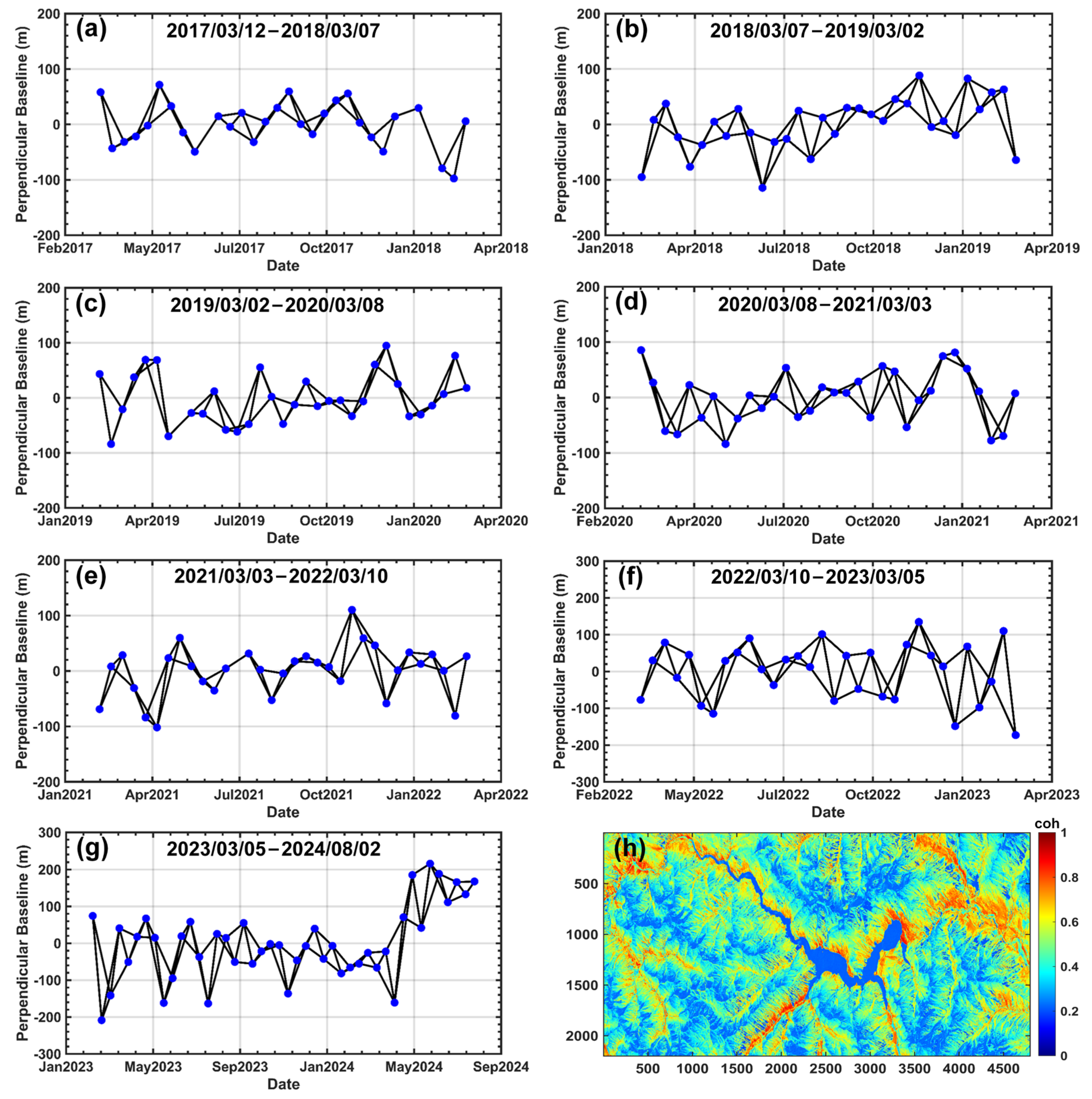
3.1.2. Interferometric Pair Combinations

For all co-registered SLC images, a baseline estimation was conducted to identify suitable interferometric pair combinations. To balance the interferometric coherence with the network density, we constrained the temporal baseline of any interferogram to ≤24 days. Tests on the full Sentinel-1 archive showed that pairs within this window maintain a median coherence of ≈0.46; extending the limit to 24–48 days decreases the median to <0.30, below the commonly accepted reliability threshold in high-relief terrain. In contrast, a stricter cap (<24 days) leaves too few interferograms for a well-conditioned SBAS inversion. Therefore, the 24-day threshold represents the optimal compromise between phase quality and temporal coverage while avoiding unnecessary computational overhead. In addition, spatial baselines of ≤350 m were adopted to maintain interferometric coherence. Given the 220 Sentinel-1 scenes and 700 km² footprint, a full-stack SBAS inversion would entail 428 interferograms and about 128 GB of RAM. To reduce hardware costs and improve efficiency while preserving short baseline quality, we processed the data in seven yearly subsets (2017–2024), each containing 50–85 interferograms. After phase unwrapping and tropospheric filtering, the yearly displacement series was concatenated into a continuous 7-year record. Tests on a 100 km² subset showed that this strategy yielded a root-mean-square difference of <1 mm/yr compared with the full-stack processing. Subsequent experiments processed the data in seven groups, with spatiotemporal baseline plots for each group, as illustrated in Figure 4a–g. The average coherence of all the interference pairs in the study area is shown in Figure 4h. Figure 4a–g depict the baseline–time network of the Sentinel-1 dataset. The blue circles correspond to every available SAR acquisition, while the black line segments link the image pairs that meet the spatial-temporal baseline thresholds and are subsequently processed as interferograms.

3.1.3. DEM Data

This study employs the SRTM 1 arc-second (SRTM GL1 V003) Digital Elevation Model (DEM), acquired during the 2000 Shuttle Radar Topography Mission (SRTM) led by NASA and the National Geospatial-Intelligence Agency (NGA) using C/X-band synthetic aperture radar interferometry. The dataset covers land areas from 60°N to 56°S with spatial resolutions of 1″ × 1″ and 3″ × 3″, referenced to the WGS84 ellipsoid (horizontal datum) and the EGM96 geoid (vertical datum). The reported absolute vertical accuracy exceeds 10 m (at the 90% confidence level), while the horizontal positioning errors remain below 20 m [44]. Subsequent reprocessing by NASA further enhanced the accuracy through noise reduction, void filling, and absolute offset correction.

Based on an analysis of regional topography and disaster-inducing factors, eight evaluation factors were selected: elevation, slope, aspect, curvature, terrain roughness, Topographic Humidity Index (THI), distance to roads, and distance to water systems. These factors were subjected to correlation analysis to construct a comprehensive evaluation framework. The elevation in the study area ranged from 2291 to 5855 m, indicating significant topographic relief. Steeper terrains are correlated with a higher susceptibility to landslides and collapses.

Utilizing 30-m SRTM DEM data, elevation was classified into six intervals: 2991–3487 m, 3487–3819 m, 3819–4138 m, 4138–4463 m, 4463–4819 m, and 4819–5855 m (Figure 5a). The slope (0–76.66°) directly indicates terrain steepness and stability, with steeper slopes being more prone to gravitational failures. Slope data derived from the 30-m SRTM DEM were categorized into six classes using the natural breaks method (Figure 5b). The aspect influences sunlight exposure, precipitation distribution, weathering, and vegetation, indirectly affecting geohazard dynamics. Aspect data were generated using surface analysis tools and divided into nine classes: flat, east, west, south, north, northeast, southeast, northwest, and southwest (Figure 5c). Curvature quantifies surface concavity and convexity, thereby impacting runoff concentration, erosion, and slope stability. Positive curvature (convex) areas correspond to ridges with dispersed runoff, while negative curvature (concave) areas represent valleys with concentrated erosion. Curvature values (−53.3 to 45.3) were classified into five intervals (Figure 5d). Terrain (0–670 m) roughness reflects slope complexity and instability, with higher roughness correlating with elevated landslide risk. Roughness is calculated as the difference between the maximum and minimum elevations within a focal window, as shown in Figure 5e.

The THI identifies areas susceptible to soil saturation and runoff accumulation. It is derived from the analysis of flow direction and accumulation using 30-m DEM data, and subsequently reclassified into six distinct intervals (Figure 5f). The Distance to Roads metric reflects human-induced disturbances, such as construction and traffic, which can destabilize slopes. Buffer zones around roads were generated and classified into various distance intervals (Figure 5g). Lastly, the Distance to Water Systems is correlated with groundwater levels and the reduction in soil shear strength. Buffers for the water systems were created and categorized (Figure 5h).

3.2. Slope Deformation Monitoring

The 428 interferometric pairs were processed using differential interferometry to generate the corresponding differential interferograms. Phase unwrapping was conducted using the minimum cost flow method [45]. Subsequently, high-quality interferograms were filtered based on their coherence and unwrapping reliability. Orbital refinement and flat-earth phase removal were performed using stable ground control points [42], followed by atmospheric phase correction [46]. The annual average deformation rates were derived using least-squares estimation, as illustrated in Figure 6. Figure 6a shows the Day-0 reference scene that establishes the spatial framework for the subsequent deformation fields, which are presented in Figure 6b onward. The red pushpins in Figure 6 were selected based on an annual average LOS deformation rate of greater than 10 cm. These points represent significant deformation magnitudes and indicate a strong potential for geological hazards to occur. Therefore, they are used as historical disaster samples for subsequent susceptibility assessment.

Spatially, the western Usoi slope (approximately 72°38′E, 38°07′–38°10′N) is identified as the most significant LOS deformation zone (the area marked by white rectan-gles in Figure 7), covering an area of approximately 4 × 6 km, with annual LOS deformation rates ranging from −210 to −480 mm/yr. Secondary LOS deformation zones, exhibiting rates between −140 and −250 mm/yr, sporadically occurred along the southern dam margin and central south-bank tributaries, encompassing areas of 1–2 km². Isolated uplift patches, with rates ranging from +100 to +300 mm/yr, were observed on the northern high-altitude slopes and glacier-covered regions, each measuring less than 1 km². The isolated uplift patches on the northern and southern high-altitude ridges coincide with active rock glacier bodies developed in continuous permafrost. Their upward LOS rates most likely reflect a superposition of long-term rock glacier creep and seasonal frost heave, processes documented elsewhere in the Pamirs and on the Tibetan Plateau. Temporally, the LOS deformation on the slope demonstrates a pattern characterized by a ’slow-fast-stable-renewed acceleration’:

• March 2017–March 2018: Initial deformation on the slope peaked at −280 mm/yr, marking the lowest intensity of deformation.
• March 2018–March 2019: Deformation intensified, reaching a peak of −375 mm/yr, with spatial expansion from north to south.
• March 2019–March 2020: Sustained high deformation persisted, peaking at −420 mm/yr, with increased uplift in the north at +250 mm/yr.
• March 2020–March 2021: A temporary slowdown occurred, peaking at −310 mm/yr, with a reduction in the extent of the deformation.
• March 2021–March 2022: Relative stability was observed, with a peak deformation rate of −340 mm/yr, indicating a brief ‘plateau phase.’
• March 2022–March 2023: Renewed acceleration was noted, peaking at −420 mm/yr, leading to the formation of linear deformation belts along the shoreline.
• March 2023–August 2024: The maximum observed deformation reached −480 mm/yr, while uplift peaked at +300 mm/yr, signaling the onset of a new active phase.

Four GNSS stations were employed to validate the InSAR results from 17 September 2022 to 30 October 2023. To minimize geometric discrepancies, GNSS-derived east-west, north-south, and vertical deformations were projected in the LOS direction. As illustrated in Figure 8, the deformation trends and inflection points obtained from InSAR closely align with the measurements from GNSS. The Root Mean Square Errors (RMSE) at all validation points are less than 3 mm, meeting the precision requirements for engineering monitoring and early warning, thereby confirming the reliability of the InSAR results.

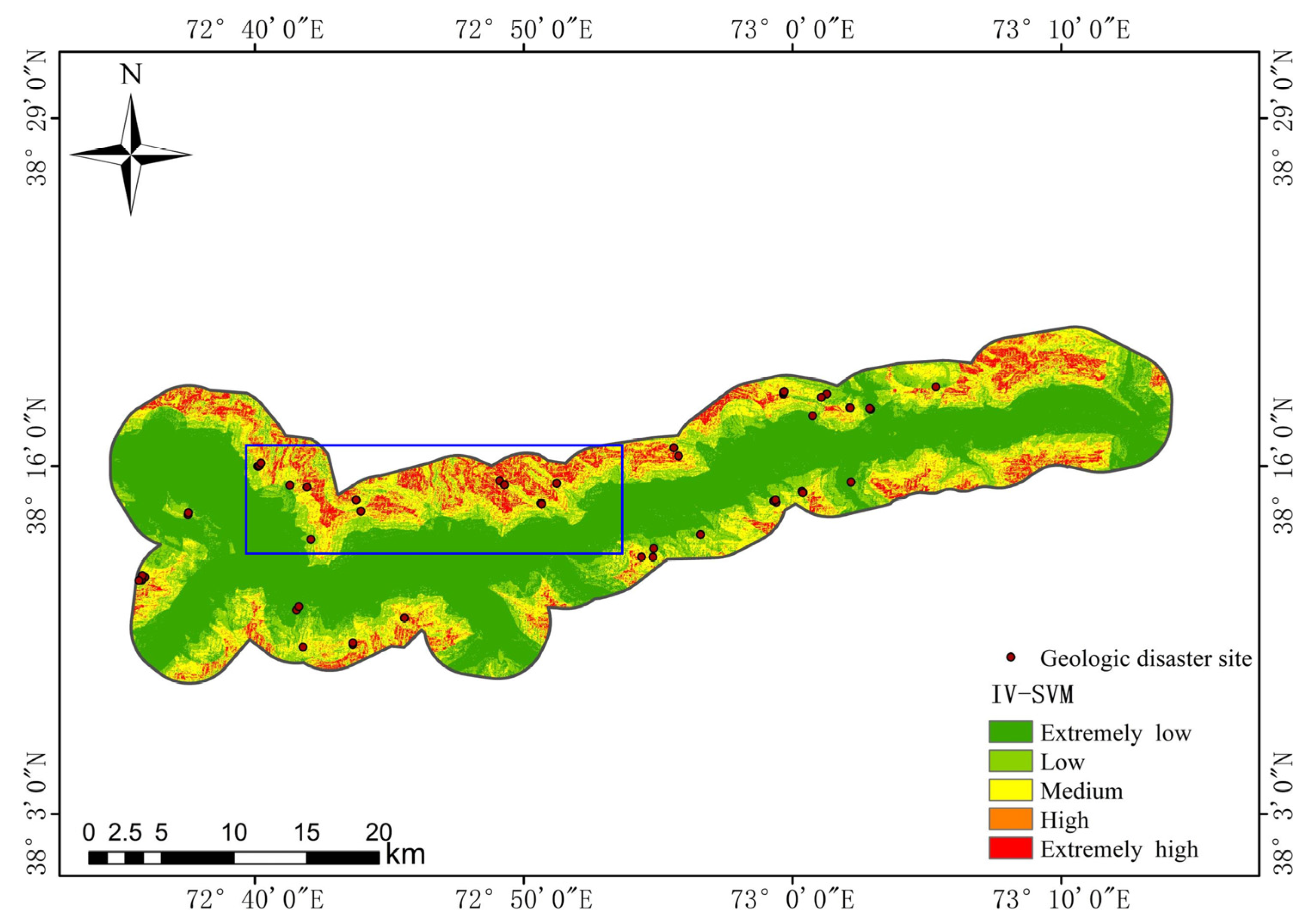
3.3. Geological Hazards Susceptibility Assessments

Landslide susceptibility assessment is a scientific process that evaluates the likelihood and potential impact of geohazards in a specific region. This assessment aims to inform disaster prevention and mitigation strategies, land-use planning, and engineering construction, ultimately reducing threats to human lives, property, and socio-economic stability. To reveal the spatial distribution characteristics and latent risks of geohazards in the study area, potential landslide points identified using InSAR technology (indicated as red high-risk points in Figure 6) were used as geohazard sample data. Eight factors were integrated into the analysis: elevation, slope, aspect, curvature, terrain roughness, THI, distance to roads, and distance to water systems (Figure 5a–g). The IV-SVM model, constructed in Section 2.2, was applied to generate a geohazard susceptibility zoning map (Figure 9), which classifies the study area into distinct susceptibility levels. The continuous susceptibility index (0–1) output by the IV-SVM model was reclassified into five categories—extremely low, low, medium, high, and extremely high—using the Jenks natural-breaks method (k = 5) [47], which optimizes intra-class homogeneity while maximizing inter-class differences. The resulting class boundaries are 0–0.20, 0.20–0.40, 0.40–0.60, 0.60–0.80, and 0.80–1.00, respectively.

Figure 9 illustrates that areas of extremely high and high susceptibility (red/orange) are distributed in a “strip and patch” pattern along both sides of the valley slopes, with their lengths fluctuating according to the meandering of the valley. The transition zones of moderate and low susceptibility (yellow and light green) encircled the outer edges of the red/orange areas, forming a “halo-like” distribution. Zones of very low susceptibility (dark green) are primarily located at the valley floor, alluvial–proluvial terraces, and gentle hillslopes.

In the western section of the Sarez Lake dammed area (72°40′E–72°55′E, the area in the blue box in Figure 9), where the valley is wide and the slopes are gentle, areas of extremely high susceptibility appear as small patches, with disaster points notably concentrated on the steep southern bank. In the central section (approximately 72°55′E–73°05′E), where valley slopes are controlled by faults and landslide deposits, the red zones are the most continuous, and the density of disaster points reaches its maximum. In the eastern section (east of 73°05′E), the valley narrows and the slope increases, resulting in the renewed intensification of extremely high-susceptibility areas. Overall, the geological hazard risk in the Sarez Lake area exhibits the characteristics of “high on both sides, low in the center” and “converging at the ends and expanding in the middle”.

Based on the geohazard susceptibility zoning results of the study area, we conducted a statistical analysis of the area percentages and counts of geohazard points across various susceptibility levels, as summarized in

Table 2. Statistical table of susceptibility partition information by IV-SVM model.

The Susceptibility Partition	Area/km2	Disaster Points/Each	Density of Disaster Points/(Each/km2)
Extremely low	201.1689	1	0.0050
low	172.4103	8	0.0464
medium	107.2800	15	0.1398
high	105.9246	17	0.1605
Extremely high	105.6528	19	0.1798

. The findings indicate that the spatial extent progressively increases from very high to very low susceptibility zones, while the number of hazard points decreases sequentially from very high to very low susceptibility zones. Furthermore, the density of hazard points (points/km²) gradually declines from very high to very low susceptibility zones.

The rationality of the geohazard susceptibility assessment results was evaluated through a statistical analysis of the percentage of geohazard points and the area coverage within each susceptibility level. Specifically, a higher percentage of geohazard points within a susceptibility level indicates a greater classification of susceptibility, while a higher susceptibility level should logically correspond to a smaller percentage of area coverage. The percentages of geohazard points and area coverage across susceptibility zones in the IV-SVM model were statistically analyzed, and the results are summarized in

Table 3. Statistical results of the proportion of disaster points and areas in the prone zoning.

The Susceptibility Partition	IV-SVM
	Proportion of Disaster Points	Proportion of Area
Extremely low	1.67%	29.05%
low	13.33%	24.90%
medium	25.00%	15.49%
high	28.33%	15.30%
Extremely high	31.67%	15.26%

.

As shown in Table 3, the IV-SVM model exhibited a progressive increase in area coverage from zones of very high to very low susceptibility. This observation aligns with the principle that higher susceptibility levels correspond to smaller spatial extents. Conversely, the proportion of geohazard points decreased from very high to very low susceptibility zones, consistent with the expectation that areas of higher susceptibility concentrate a greater proportion of hazard points. A comprehensive analysis confirms that the IV-SVM model satisfies all rationality validation criteria. Table 2 and Table 3 present the spatial distributions of the susceptibility zones derived from the IV-SVM model. The very high susceptibility zone occupies the smallest area, approximately 105.65 km² (15.26% of the total study area), and contains 19 geohazard points (31.67% of the total) with a density of 0.1798 points/km². The high-susceptibility zone covers 105.92 km² (15.30% of the total area), with 17 geohazard points (28.33% of the total) at a density of 0.1605 points/km². The moderate susceptibility zone spans 107.28 km² (15.49% of the total area), encompassing 15 geohazard points (25.00% of the total) with a density of 0.1398 points/km². The low-susceptibility zone covers 172.41 km² (24.90% of the total area), containing eight geohazard points (13.33% of the total) at a density of 0.0464 points/km². The very low susceptibility zone, the largest in extent at 201.17 km² (29.05% of the total area), included only one geohazard point (1.67% of the total) with a density of 0.005 points/km².

4. Discussion

The IV-SVM landslide susceptibility assessment method introduces an information model to screen the influencing factors and optimize the sample set prior to SVM modeling. Firstly, the information model is employed to calculate the contribution of various environmental factors to landslide occurrence, allowing for the removal of redundant factors with low information content and weak relationships with landslides. This reduction simplifies the model and mitigates the risk of overfitting. Subsequently, based on the evaluation results of the information content, prone areas are delineated, and negative sample points are selectively chosen from low-prone areas to alleviate the interference of sample imbalance on the SVM decision hyperplane. This approach effectively addresses the sensitivity of the SVM to the distribution of the training data. When landslide samples are imbalanced with non-landslide samples, the classification hyperplane tends to favor the dominant categories, leading to a decreased recognition rate for minority classes, such as landslide occurrences. Overall, this method enhances the accuracy and universality of our model.

To further validate the superiority and enhanced prediction accuracy of the IV-SVM model in assessing geological hazard-prone areas of the Pamir Plateau, we selected 60 potential geological hazard points identified through InSAR within the study area. Additionally, 180 random non-geological hazard points were generated at a 1:3 ratio to create an SVM evaluation sample set for training. The distribution of negative samples for non-geological hazards is shown in Figure 10. The selected eight-factor attribute values were extracted from the sample dataset, which was subsequently utilized for training and prediction in a 7:3 ratio. The final trained model was employed to predict the entire study area, resulting in a geological hazard susceptibility index for the region. This index was categorized into five groups based on the natural discontinuity method: extremely high, high, medium, low, and extremely low susceptibility areas. The evaluation results are shown in Figure 11.

Based on the geohazard susceptibility zoning results derived from the SVM model, this study statistically analyzes the distribution of areas and density of hazard points across various susceptibility levels, as summarized in

Table 4. Statistical results of susceptibility partition information using SVM.

The Susceptibility Partition	Area/km2	Disaster Points/Each	Density of Disaster Points/(Each/km2)
Extremely low	343.6722	5	0.0145
low	163.6893	9	0.0550
medium	90.8685	14	0.1541
high	57.4047	14	0.2439
Extremely high	36.8019	18	0.4891

. The results indicate a progressive decrease in hazard point density from very high-to very low-susceptibility zones, while the area coverage gradually increases from very high-to very low-susceptibility zones. This inverse relationship between susceptibility levels, spatial extent, and hazard concentration was consistent with the findings of the IV-SVM model.

To evaluate the rationality of the SVM and IV-SVM model results, we statistically compared the percentages of hazard points and area coverage across susceptibility zones, as shown in Figure 12a,b. Figure 12a indicates that the SVM model identifies 54% of the hazard points within the very high- and high-risk zones, while the IV-SVM model captures 63% of the hazard points in these areas, reflecting an improvement in the detection of approximately 9%. Figure 12b shows that around 7% of the hazard points (1 out of 14 total) are misclassified into the very low-risk zone by the SVM model, which encompasses 50% of the study area, highlighting a significant number of false positives. In contrast, the IV-SVM model misclassifies only about 2% of the hazard points into the very low-risk zone, which constitutes 29% of the area, thereby reducing misclassification by five percentage points.

To comparatively analyze the accuracy of the SVM and IV-SVM model results, this study employed Receiver Operating Characteristic (ROC) curves to evaluate the precision of geohazard susceptibility zoning. The predictive outcomes of both the SVM and IV-SVM models were treated as independent variables, while geohazard points (assigned a binary value of 1) and non-geohazard points (assigned a value of 0) served as the dependent variables. The ROC curves for both models are shown in Figure 13. The results demonstrate that the SVM model achieves an AUC value of 0.87, whereas the IV-SVM model attains a higher AUC value of 0.97, indicating superior predictive accuracy and evaluation efficacy for geohazard susceptibility assessment in the study area. Therefore, both rationality validation and accuracy verification confirm that the IV-SVM model is more suitable than the SVM model for geohazard susceptibility evaluation in the study area.

Compared to the traditional SVM risk assessment model, the IV-SVM model exhibits more scientifically and rationally defined partitioning characteristics in both accuracy and rationality tests. This enhancement not only increases the clustering degree of disaster points but also preserves the economic efficiency of the area allocation. Furthermore, the AUC of the IV-SVM model reached 0.97, which is approximately 11.5% higher than that of the SVM model. The IV-SVM model preliminarily addressed the issues of false alarms and missed identifications of disaster points caused by the excessive subdivision of extremely low-risk areas inherent in traditional SVM models, thereby improving the reliability of geological hazard risk zoning results. Notably, the extremely low-risk area contains only a small number of disaster points, while the extremely high-risk area, despite being the smallest in size, has the highest concentration of disaster points. This further corroborates the effective identification capability of the IV-SVM model for hazardous hotspots.

The deformation monitoring and stability assessment of the Sarez barrier lake slope from 2017 to 2024 revealed a spatial pattern of landslide susceptibility risk characterized by a “strong west and weak east” trend (Figure 6a–g). While some regions demonstrate uplift, the amplitude remains minimal, and the distance from the water body is considerable, resulting in limited implications for the safety of the barrier lake. Temporally, the deformation presents a rhythm of “slow-fast-stable-fast”(Figure 6a–g): it accelerated between 2017/18 and 2019/20 (Figure 6b–d), briefly stabilized from 2020/21 to 2021/22 (Figure 6e,f), and then accelerated again starting in 2022 (Figure 6g). The maximum settlement rate shows a stepwise increase (−280 → −375 → −420 → −480 mm/yr), suggesting that the landslide may have entered a new acceleration phase.

Although the present study extends the deformation record to 2024 and refines the IV-SVM susceptibility model, three constraints remain: (i) single-geometry data—only descending-track Sentinel-1 scenes were available, precluding full 3-D displacement recovery and possible lateral motion; (ii) incomplete forcing factors—critical drivers such as groundwater fluctuations and freeze–thaw cycles were not explicitly incorporated, potentially masking causative links; and (iii) limited outward transferability—the workflow and data have not yet been released in an open, easily replicable package, restricting adoption at other high-altitude barrier lakes.

In the future, collaborative monitoring of multi-source datasets will be facilitated by the continuous acquisition of SAR data and high-resolution optical images. Moreover, coupling the newly acquired deformation data with environmental factors, such as groundwater levels and freeze-thaw indices, will further enhance the accuracy of the geological hazard risk assessment model. Furthermore, by making datasets accessible, publishing technical white papers, and conducting local training courses, we can promote the sharing of achievements and build regional capacity. This methodological system can then be extended to other mountainous barrier lakes, providing aerospace information support for disaster prevention and reduction in the high-altitude barrier lakes of the Pamir Plateau, where data are scarce.

5. Conclusions

This study couples SBAS-InSAR deformation monitoring with an IV-SVM susceptibility model to deliver an end-to-end, real-time, early warning framework for dammed-lake hazards. The main conclusions are as follows:

(1)

From March 2017 to August 2024, slope displacement around Sarez Lake shows a persistent west-greater-than-east pattern; some areas exceed 200 mm/yr of deformation, and their peak rates rise stepwise with time.

(2)

Susceptibility zoning reveals a “high-flank/low-center” pattern: 15.3% of the area is classified as extremely high risk, whereas extremely low-risk zones occupy 29.1%; recorded hazard density drops correspondingly from 0.180 to 0.005 events km⁻².

(3)

The accelerating deformation of the slope indicates that the landslide mass may be approaching a new acceleration phase, threatening the dam shoulder stability. Therefore, continuous high-precision GNSS and multi-source SAR/optical monitoring at critical points are urgently required.

References

1. Dai, F.C.; Lee, C.F.; Deng, J.H.; Tham, L.G. The 1786 earthquake-triggered landslide dam and subsequent dam-break flood on the Dadu River, southwestern China. Geomorphology 2005, 65, 205–221. [Google Scholar] [CrossRef]
2. Mantovani, F.; Vita-Finzi, C. Neotectonics of the Vajont dam site. Geomorphology 2003, 54, 33–37. [Google Scholar] [CrossRef]
3. Zhu, C.; Zhang, X.; Fang, H.; Wang, W. Dammed Lake Water Volume estimation by satellite imagery and digital elevation model Under Unknown Underwater Terrain Scenario. Nat. Remote Sens. Bull. 2022, 26, 148–154. [Google Scholar] [CrossRef]
4. Li, J.; Zhang, X.; Chen, Y.; Zhu, C.; Wei, W. The Lowest-Cost Route and feasibility Analysis for Eastward Water Diversion from Lake Sare. J. Nat. Disaster 2021, 30, 159–167. [Google Scholar]
5. Tsou, C.-Y.; Feng, Z.-Y.; Chigira, M. Catastrophic landslide induced by Typhoon Morakot, Shiaolin, Taiwan. Geomorphology 2011, 127, 166–178. [Google Scholar] [CrossRef]
6. Liu, Z.; Chen, Q.; Li, X.; Chen, C.; Zhou, C.; Wang, C. A review of the research on the failure potential of landslide dams caused by overtopping and seepage. Nat. Hazards 2023, 116, 1375–1408. [Google Scholar] [CrossRef]
7. Fan, X.; Dufresne, A.; Subramanian, S.S.; Strom, A.; Hermanns, R.L.; Stefanelli, C.T.; Hewitt, K.; Yunus, A.T.; Dunning, S.; Capra, L. The formation and impact of landslide dams—State of the art. Earth-Sci. Rev. 2020, 203, 103–116. [Google Scholar] [CrossRef]
8. Shi, Z.; Guan, S.; Peng, M.; Zhang, L.; Zhu, Y.; Cai, Q. Cascading breaching of the Tangjiashan landslide dam and two smaller downstream landslide dams. Eng. Geol. 2015, 193, 445–458. [Google Scholar] [CrossRef]
9. Guo, C.; Montgomery, D.R.; Zhang, Y.; Zhong, N.; Fan, C.; Wu, R.; Yang, Z.; Ding, Y.; Jin, J.; Yan, Y. Evidence for repeated failure of the giant Yigong landslide on the edge of the Tibetan Plateau. Sci. Rep. 2020, 10, 14371. [Google Scholar] [CrossRef]
10. Veh, G.; Korup, O.; Walz, A. Hazard from Himalayan glacier lake outburst floods. Proc. Natl. Acad. Sci. USA 2020, 117, 907–912. [Google Scholar] [CrossRef]
11. Schuster, R.L.; Alford, D. Usoi landslide dam and Lake Sarez, Pamir Mountains, Tajikistan. Environ. Eng. Geosci. 2004, 10, 151–168. [Google Scholar] [CrossRef]
12. Risley, J.C.; Walder, J.S.; Denlinger, R.P. Usoi Dam wave overtopping and flood routing in the Bartang and Panj Rivers, Tajikistan. Nat. Hazards 2006, 38, 375–390. [Google Scholar] [CrossRef]
13. Deng, X.; Li, Y.; Zhang, J.; Kong, L.; Abuduwaili, J.; Gulayozov, M.; Kodirov, A.; Ma, L. The Role of Atmospheric Circulation Patterns in Water Storage of the World’s Largest High-Altitude Landslide-Dammed Lake. Atmosphere 2025, 16, 209. [Google Scholar] [CrossRef]
14. Alford, D.; Cunha, S.F.; Ives, J.D. Lake Sarez, Pamir Mountains, Tajikistan: Mountain Hazards and Development Assistance. Mt. Res. Dev. 2000, 20, 20–23. [Google Scholar] [CrossRef]
15. Ishuk, N.R.; Ishuk, A.R. Once Again on the Problems of Lake Sarez. In Proceedings of the International Conference “Experience in Studying Landslides and Rockfalls in the Territory of Tajikistan and Methods of Engineering Protection”, Dushanbe, Tajikistan, 26–27 September 2002. [Google Scholar]
16. Ischuk, A.R. Natural and Artificial Rockslide Dams; Springer: Berlin/Heidelberg, Germany, 2011; pp. 423–440. [Google Scholar]
17. Nardini, O.; Confuorto, P.; Intrieri, E.; Montalti, R.; Montanaro, T.; Garcia Robles, J.; Poggi, F.; Raspini, F. Integration of satellite SAR and optical acquisitions for the characterization of the Lake Sarez landslides in Tajikistan. Landslides 2024, 21, 1385–1401. [Google Scholar] [CrossRef]
18. World Bank. Project Appraisal Document on a Proposed Grant to the Republic of Tajikistan for a Lake Sarez Risk Mitigation Project; The World Bank: Washington, DC, USA, 2004. [Google Scholar]
19. United Nations International Strategy for Disaster Reduction. Sarez Lake: The Latest Achievements and Unsolved Problems; UNISDR Central Asia Office: Dushanbe, Tajikistan, 2009; Available online: https://www.undrr.org/publication/sarez-lake-latest-achievements-and-unresolved-problems (accessed on 18 May 2025).
20. Han, J.; Tu, R.; Lu, X.; Fan, L.; Zhuang, W.; Wang, W.; Zhao, F.; Dalai, B.; Shonazarovich, G.M.; Safarov, M. Analysis of BDS/GPS Deformation Monitoring for the Lake Sarez Dam. Remote Sens. 2023, 15, 4773. [Google Scholar] [CrossRef]
21. Grebby, S.; Sowter, A.; Gee, D.; Athab, A.; Barreda-Bautista, B.D.; Girindran, R.; Marsh, S. Remote monitoring of groundmoti-on hazards in high-mountain terrain using optical sub-pixel correlation: A case study of Lake Sarez, Tajikistan. Appl. Sci. 2021, 11, 8738. [Google Scholar] [CrossRef]
22. Bekaert, D.P.; Handwerger, A.L.; Agram, P.; Kirschbaum, D.B. InSAR-based detection method for mapping and monitoring slow-moving landslides in remote regions with steep and mountainous terrain: An application to Nepal. Remote Sens. Environ. 2020, 249, 111983. [Google Scholar] [CrossRef]
23. Cook, M.E.; Brook, M.S.; Hamling, I.J.; Cave, M.; Tunnicliffe, J.F. Investigating slow-moving shallow soil landslides using Sentinel-1 InSAR data in Gisborne, New Zealand. Landslides 2023, 20, 427–446. [Google Scholar] [CrossRef]
24. Liu, X.J.; Zhao, C.Y.; Zhang, Q.; Lu, Z.; Li, Z.H.; Yang, C.S.; Zhu, W.; Zeng, J.L.; Chen, L.Q.; Liu, C.J. Integration of Sentinel-1 and Alos/Palsar-2 Sar Datasets for Mapping Active Landslides Along the Jinsha River Corridor, China. Eng. Geol. 2021, 284, 106033. [Google Scholar] [CrossRef]
25. Liu, X.K.; Shao, S.; Shao, S. Landslide susceptibility zonation using the Analytical Hierarchy Process (AHP) in the Great Xi’an Region, China. Sci. Rep. 2024, 14, 2941. [Google Scholar] [CrossRef]
26. Conoscenti, C.; Ciaccio, M.; Caraballo-Arias, N.A.; Gómez-Gutiérrez, Á.; Rotigliano, E.; Agnesi, V. Assessment of susceptibility to earth-flow landslides using logistic regression and multivariate adaptive regression splines: A case of the Belice River basin (western Sicily, Italy). Geomorphology 2015, 242, 49–64. [Google Scholar] [CrossRef]
27. Wubalem, A.; Meten, M. Landslide susceptibility mapping using information value and logistic regression models in Goncha Siso Eneses area, northwestern Ethiopia. SN Appl. Sci. 2020, 2, 807. [Google Scholar] [CrossRef]
28. Yao, X.; Tham, L.; Dai, F. Landslide susceptibility mapping based on support vector machine: A case study on natural slopes of Hong Kong, China. Geomorphology 2008, 101, 572–582. [Google Scholar] [CrossRef]
29. Shirvani, Z. A holistic analysis for landslide susceptibility mapping applying geographic object-based Random Forest. Remote Sens. 2020, 12, 434. [Google Scholar] [CrossRef]
30. El Jazouli, A.; Barakat, A.; Khellouk, R. GIS-multicriteria evaluation using the AHP for landslide susceptibility mapping in Oum Er Rbia high basin (Morocco). Geoenviron. Disasters 2019, 6, 3. [Google Scholar] [CrossRef]
31. Lee, S. Cross-verification of spatial logistic regression for landslide susceptibility analysis: A case study of Korea. In Proceedings of the 31st International Symposium on Remote Sensing of Environment, ISRSE 2005: Global Monitoring for Sustainability and Security, St. Petersburg, Russia, 20–24 June 2005. [Google Scholar]
32. Merghadi, A.; Yunus, A.P.; Dou, J.; Whiteley, J.; ThaiPham, B.; Bui, D.T.; Avtar, R.; Abderrahmane, B. Machine learning methods for landslide susceptibility studies: A comparative overview of algorithm performance. Earth-Sci. Rev. 2020, 207, 103225. [Google Scholar] [CrossRef]
33. Kulsoom, I.; Hua, W.; Hussain, S.; Chen, Q.; Khan, G.; Shihao, D. SBAS-InSAR based validated landslide susceptibility mapping along the Karakoram Highway: A case study of Gilgit-Baltistan, Pakistan. Sci. Rep. 2023, 13, 3344. [Google Scholar] [CrossRef]
34. Achu, A.L.; Aju, C.D.; Di Napoli, M.; Prakash, P.; Gopinath, G.; Shaji, E.; Chandra, V. Machine-learning based landslide susceptibility modelling with emphasis on uncertainty analysis. Geosci. Front. 2023, 14, 101657. [Google Scholar] [CrossRef]
35. Tzampoglou, P.; Loukidis, D.; Anastasiades, A.; Tsangaratos, P. Advanced machine learning techniques for enhanced landslide susceptibility mapping: Integrating geotechnical parameters in the case of Southwestern Cyprus. Earth Sci. Inform. 2025, 18, 357. [Google Scholar] [CrossRef]
36. Pradhan, A.M.S.; Kim, Y. Spatial data analysis and application of evidential belief functions to shallow landslide susceptibility mapping at Mt. Umyeon, Seoul, Korea. Bull. Eng. Geol. Environ. 2017, 76, 1263–1279. [Google Scholar] [CrossRef]
37. Liu, S.; Wang, L.; Zhang, W.; He, Y.; Pijush, S. A comprehensive review of machine learning-based methods in landslide susceptibility mapping. Geol. J. 2023, 58, 2283–2301. [Google Scholar] [CrossRef]
38. Youssef, K.; Shao, K.; Moon, S.; Bouchard, L.S. Landslide susceptibility modeling by interpretable neural network. Commun. Earth Environ. 2023, 4, 162. [Google Scholar] [CrossRef]
39. Ballabio, C.; Sterlacchini, S. Support vector machines for landslide susceptibility mapping: The Staffora River Basin case study, Italy. Math. Geosci. 2012, 44, 47–70. [Google Scholar] [CrossRef]
40. Liu, Y.; Xu, Y.; Huang, J.; Liu, H.; Fang, Y.; Yu, Y. A comparative study of intelligent prediction models for landslide susceptibility: Random forest and support vector machine. Front. Earth Sci. 2024, 12, 1519771. [Google Scholar] [CrossRef]
41. Berardino, P.; Fornaro, G.; Lanari, R.; Sansosti, E. A new algorithm for surface deformation monitoring based on small baseline differential SAR interferograms. IEEE Trans. Geosci. Remote Sens. 2002, 40, 2375–2383. [Google Scholar] [CrossRef]
42. Hanssen, R.F. Radar Interferometry: Data Interpretation and Error Analysis; Springer: Dordrecht, The Netherlands, 2001. [Google Scholar]
43. Cortes, C.; Vapnik, V. Support-vector networks. Mach. Learn. 1995, 20, 273–297. [Google Scholar] [CrossRef]
44. Rodriguez, E.; Morris, C.S.; Belz, J.E. A global assessment of the SRTM performance. Photogramm. Eng. Remote Sens. 2006, 72, 249–260. [Google Scholar] [CrossRef]
45. Costantini, M. A novel phase unwrapping method based on network programming. IEEE Trans. Geosci. Remote Sens. 1998, 36, 813–821. [Google Scholar] [CrossRef]
46. Yu, C.; Li, Z.; Penna, N.T.; Crippa, P. Generic Atmospheric Correction Model for Interferometric Synthetic Aperture Radar Observations. J. Geophys. Res. Solid Earth 2018, 123, 9202–9222. [Google Scholar] [CrossRef]
47. Jenks, G.F. The Data Model Concept in Statistical Mapping. Int. Yearb. Cartogr. 1967, 7, 186–190. [Google Scholar]
Figure 1. Geographical location map of the study area. The horizontal measurement accuracy of GNSS monitoring points is about 2.5 mm, and the elevation measurement accuracy is about 5 mm.
Remotesensing 17 02300 g001
Figure 2. The framework of deformation monitoring and geological hazard susceptibility assessment on slopes of Sarez Barrier Lake in the Pamir Plateau.
Remotesensing 17 02300 g002
Figure 3. Schematic diagram of the SVM model, the red and blue points denote the support vectors of the positive and negative classes.
Remotesensing 17 02300 g003
Figure 4. The distribution of spatial-temporal baseline (ag) and mean coherence map (h), (ag) blue circles denote individual SAR scenes plotted at their perpendicular baseline relative to the reference (master) image. Black line segments connect two scenes that form an interferometric pair retained in the SBAS network after applying spatial-temporal baseline thresholds.
Remotesensing 17 02300 g004
Figure 5. Grading chart of each susceptibility evaluation factor.
Remotesensing 17 02300 g005
Figure 6. The average deformation rate for each year from March 2017 to August 2024, with red pushpins indicating potential high-risk geological hazard sites and white rectangles indicating locations with severe deformation. The reference amplitude image (T0 = 12 March 2017) is provided solely for context and contains no deformation information. See Supplementary Materials for additional color scale ranges.
Remotesensing 17 02300 g006
Figure 7. Enlarged view of the white rectangles in Figure 6.
Remotesensing 17 02300 g007
Figure 8. Comparison of deformation monitoring results between InSAR and GNSS.
Remotesensing 17 02300 g008
Figure 9. Results of Landslides susceptibility evaluation by IV-SVM model.
Remotesensing 17 02300 g009
Figure 10. Distribution of negative samples of non-geological disasters.
Remotesensing 17 02300 g010
Figure 11. Landslides geological disasters susceptibility mapping using SVM.
Remotesensing 17 02300 g011
Figure 12. Reasonability and susceptibility evaluation for SVM and IV-SVM models: (a) distribution of disaster sites across zones for different models; (b) area percentage of each zone for different models.
Remotesensing 17 02300 g012
Figure 13. The comparison of ROC curves between SVM and IV-SVM models. The black dashed line is the “chance” or “no-skill” reference line. It marks the performance of a random classifier where the true-positive rate equals the false-positive rate (AUC = 0.50). Any ROC curve that stays above this line indicates a model that performs better than random guessing.
Remotesensing 17 02300 g013