Article

Comparative Analysis of Multi-Platform, Multi-Resolution, Multi-Temporal LiDAR Data for Forest Inventory

1
Lyles School of Civil Engineering, Purdue University, West Lafayette, IN 47907, USA
2
Department of Forestry and Natural Resources, Purdue University, West Lafayette, IN 47907, USA
*
Author to whom correspondence should be addressed.
Remote Sens. 2022, 14(3), 649; https://doi.org/10.3390/rs14030649
Submission received: 22 December 2021 / Revised: 19 January 2022 / Accepted: 27 January 2022 / Published: 29 January 2022

Abstract

:
LiDAR technology is rapidly evolving as various new systems emerge, providing unprecedented data to characterize forest vertical structure. Data from different LiDAR systems present distinct characteristics owing to a combined effect of sensor specifications, data acquisition strategies, as well as forest conditions such as tree density and canopy cover. Comparative analysis of multi-platform, multi-resolution, and multi-temporal LiDAR data provides guidelines for selecting appropriate LiDAR systems and data processing tools for different research questions, and thus is of crucial importance. This study presents a comprehensive comparison of point clouds from four systems, linear and Geiger-mode LiDAR from manned aircraft and multi-beam LiDAR on unmanned aerial vehicle (UAV), and in-house developed Backpack, with the consideration of different forest canopy cover scenarios. The results suggest that the proximal Backpack LiDAR can provide the finest level of information, followed by UAV LiDAR, Geiger-mode LiDAR, and linear LiDAR. The emerging Geiger-mode LiDAR can capture a significantly higher level of detail while operating at a higher altitude as compared to the traditional linear LiDAR. The results also show: (1) canopy cover percentage has a critical impact on the ability of aerial and terrestrial systems to acquire information corresponding to the lower and upper portions of the tree canopy, respectively; (2) all the systems can obtain adequate ground points for digital terrain model generation irrespective of canopy cover conditions; and (3) point clouds from different systems are in agreement within a ±3 cm and ±7 cm range along the vertical and planimetric directions, respectively.

1. Introduction

Global forest ecosystems, covering around 30% of the land surface, can provide various critical ecosystem services such as maintaining global carbon balance, mitigating climate change, and promoting economic and social development [1,2]. Accurate inventory is essential for better understanding and for the management of forest ecosystems from local to global scales. Along with the development of platforms, sensors, and processing technologies, remote sensing has been widely used for forest mapping and inventory. For example, Landsat scenes are used for forest mapping at a regional scale [3,4]; multispectral Sentinel-2 imagery are adopted to estimate nation-wide canopy height [5]; and very high-resolution satellite, aerial, and unmanned aerial vehicle (UAV) imagery are acquired for tree counting and localization [6,7]. Because satellite and aerial imagery only provides the top view perspective, it is more challenging to use such data to investigate forest vertical structure for the derivation of inventory metrics such as tree height and crown depth. LiDAR, on the other hand, is effective for deriving such metrics because it provides direct 3D measurements [8,9,10].
As various technologies evolve, airborne LiDAR, UAV LiDAR, and proximal (e.g., static terrestrial and Backpack) LiDAR are becoming increasingly available; thus, expanding its applications in forest inventory. Airborne LiDAR—including conventional linear LiDAR and emerging Geiger-mode LiDAR—is commonly used for derivation of forest metrics such as digital terrain model (DTM), tree height, and crown structure at a regional scale [11,12,13]. In spite of its limited spatial coverage, UAV LiDAR provides a higher resolution than its manned, airborne counterpart at a lower cost. The close sensor-to-object distance allows for higher penetration ability, facilitating fine-scale forest inventory (e.g., tree counting and segmentation) [14]. Compared to the above modalities, proximal, in-canopy LiDAR mapping is time-consuming but provides a higher level of detail of internal forest structure (e.g., individual tree detection and localization, stem segmentation, and diameter measurement) [15,16]. Each of the above LiDAR modalities has its own advantages and limitations. Down-looking airborne and UAV LiDAR systems provide highly accurate data for tree canopy description but lack tree trunk information [17]. Terrestrial laser scanning (TLS) provides very high-resolution data below the canopy; however, it suffers from occlusions, which require the acquisition of multiple overlapping scans that have to be registered. Therefore, TLS data acquisition is highly time-consuming and not easily scalable [18,19]. Proximal, mobile LiDAR systems (e.g., Backpack-mounted LiDAR) capture detailed tree trunk information with high efficiency. However, deriving accurate trajectory for such systems remains challenging due to the intermittent access to Global Navigation Satellite System (GNSS) signal under the canopy. In addition, the limited vertical field of view and measurement range of proximal systems may result in missing the upper canopy [16,20].
The varying characteristics of multi-platform, multi-resolution, and multi-temporal LiDAR data underline the need to perform comparative analysis for forest inventory. LiDAR systems with large spatial coverage (e.g., satellite and manned aircraft systems) are ideal for regional canopy height model generation, while small footprint LiDAR from low-altitude flights provides fine resolution for individual tree isolation [21,22,23]. Yu et al. [24] compared two airborne LiDAR systems (ALS)—single-photon Geiger-mode LiDAR and multi-photon linear LiDAR—in terms of their potential in characterizing ground and forest attributes. They concluded that the Geiger-mode LiDAR can deliver forest attribute estimates with accuracy comparable to those from linear LiDAR while operating at a much higher altitude, thus enabling forest mapping at a national scale. Several studies compared ALS and TLS and demonstrated their comparable capacity to derive forest measurements such as canopy height, canopy cover, and leaf area [20,25]. Prior research also highlighted the complementary nature of ALS and TLS data in forest inventory: the former delineates upper-canopy structure with a broad spatial extent while the latter provides fine resolution measurements for characterizing forest vertical structure at a stand level [25,26]. Crespo-Peremarch et al. [27] studied the use of full-waveform and discrete airborne as well as discrete terrestrial laser scanning data for studying forest vertical distribution; they stated that full-waveform airborne LiDAR have better capability in representing tree vertical structure than discrete airborne LiDAR, leading to very similar results to TLS. UAV LiDAR was also compared to ALS and TLS in terms of the quality of derived point cloud data [28]. The main advantage of UAV LiDAR when compared to TLS is the more homogenous point distribution and top perspective of the former, leading to more accurate canopy height estimation [29]. However, UAV flights under full-leaf cover limit the level of detail at the lower canopy level. Therefore, flying over forests under leaf-off conditions is still favorable when DTM or wood volume are the variables of interest [30]. Hyyppä et al. [31] evaluated the comparative performance of Backpack, handheld, under-canopy UAV, and above-canopy UAV LiDAR systems. Their study revealed that ground-based and under-canopy mobile LiDAR systems provide promising results for individual tree parameters derivation; whereas the accuracy of above-canopy UAV LiDAR systems is not yet sufficient for predicting stem attributes of individual trees for forest inventory with a high accuracy. Regardless of the used modality, multi-temporal LiDAR data are essential for understanding the dynamics of forests, such as forest structure, tree growth, species mapping, and carbon monitoring [32,33,34]. Although many studies have investigated multi-platform, multi-resolution, and multi-temporal LiDAR systems, comprehensive comparative analysis that includes a wide range of remote sensing modalities, discusses the impact of canopy cover, and focuses on forest inventory capabilities, has not been sufficiently covered.
In this paper, multi-platform, multi-resolution, and multi-temporal LiDAR datasets over a forest plantation are analyzed for better understanding of their characteristics and the impact of data quality on forest inventory results. Comparative analysis of available and acquired datasets is performed in terms of point cloud characteristics, point cloud quality, and ability to derive forest inventory metrics. The key contributions are summarized as follows:
  • A wide range of LiDAR modalities, including linear and Geiger-mode LiDAR from manned aircraft systems, and multi-beam LiDAR from UAV and Backpack systems, are analyzed.
  • A comprehensive investigation of point cloud characteristics and geolocation accuracy is conducted, laying the foundations of multi-platform, multi-resolution, and multi-temporal data fusion.
  • A comparative analysis that focuses on forest inventory capabilities and discusses the effect of canopy cover is presented, providing directions for selecting appropriate LiDAR modalities and data processing tools for different applications.
The remainder of this paper is structured as follows: first, different LiDAR modalities and acquired data descriptions are provided; then, the adopted methodology used for the comparative analysis of the characteristics of different LiDAR datasets is discussed; detailed analysis of the investigated characteristics as derived from the LiDAR datasets are covered afterwards; finally, discussions and study conclusions are presented.

2. Data Acquisition Systems and Datasets Description

Several datasets were acquired for this study using different LiDAR systems; namely, linear and Geiger-mode (single-photon or flash) LiDAR from manned aircraft systems, and multi-beam LiDAR from UAV and proximal Backpack systems. The Geiger-mode LiDAR data were provided by VeriDaas Corporation (Denver, CO, USA), while the linear LiDAR data were available through the state-wide coverage of the United States Geological Survey (USGS) 3-D Elevation Program (3DEP). The UAV and proximal LiDAR data were captured by in-house developed systems within the Digital Photogrammetry Research Group at Purdue University. This section starts with introducing the different LiDAR modalities and platforms. It then describes the study site and datasets used in this study.

2.1. Mobile LiDAR Systems

2.1.1. Linear LiDAR

Linear LiDAR, which is used by the majority of airborne systems, is based on emitted laser pulses of some nanosecond pulse width at wavelengths from 500 nm (for bathymetric LiDAR) to 1.5 μm (for topographic LiDAR), and the echo returns are then digitized. The output current of the Avalanche Photodiode (APD) detector is proportional to the input optical power. Survey-grade systems use a single laser. To discriminate between signal return and noise, traditional linear LiDAR utilizes a single detector that requires a flux of 500 to 1000 photons to detect the return signal. To provide coverage across the swath, a deflecting mirror is used. Depending on the type of the mirror used, the LiDAR would be scanning in either elliptical, parallel, zigzag, or sinusoidal pattern, as depicted in Figure 1a. To derive point clouds in the mapping coordinate system, a linear LiDAR system is also equipped with a position and orientation unit—an integrated Global Navigation Satellite System/Inertial Navigation System (GNSS/INS) unit. The majority of LiDAR data captured for national coverage (e.g., the USGS 3DEP data) are based on linear LiDAR systems.

2.1.2. VeriDaaS Geiger-Mode LiDAR System

The VeriDaaS system [35] uses a Geiger-mode LiDAR sensor in conjunction with an Applanix POS AV 610 for direct georeferencing. The Geiger-mode LiDAR is a relatively new technology as compared to the traditional linear LiDAR. The Geiger-mode LiDAR sensor consists of arrays of Geiger-mode Avalanche Photodiode (GmAPD) detectors. Each of the GmAPD detectors is capable of detecting the return signal with a few photons [36]. The extreme sensitivity of GmAPD detectors allows the design of LiDAR systems that operate at a lower energy, higher altitude, and faster flying speed, and acquire measurements in a much higher density compared to linear LiDAR systems [37,38]. The VeriDaaS system has an array of 32 by 128 GmAPD detectors, which effectively collects 204,800,000 observations per second with a pulse repetition rate of 50 kHz. The use of a Palmer scanner, together with a 15-degree scan angle of the laser and scan pattern of a 50% swath overlap, enables multi-view data collection, which aids in minimizing occlusions and shadowing, as shown in Figure 1b.

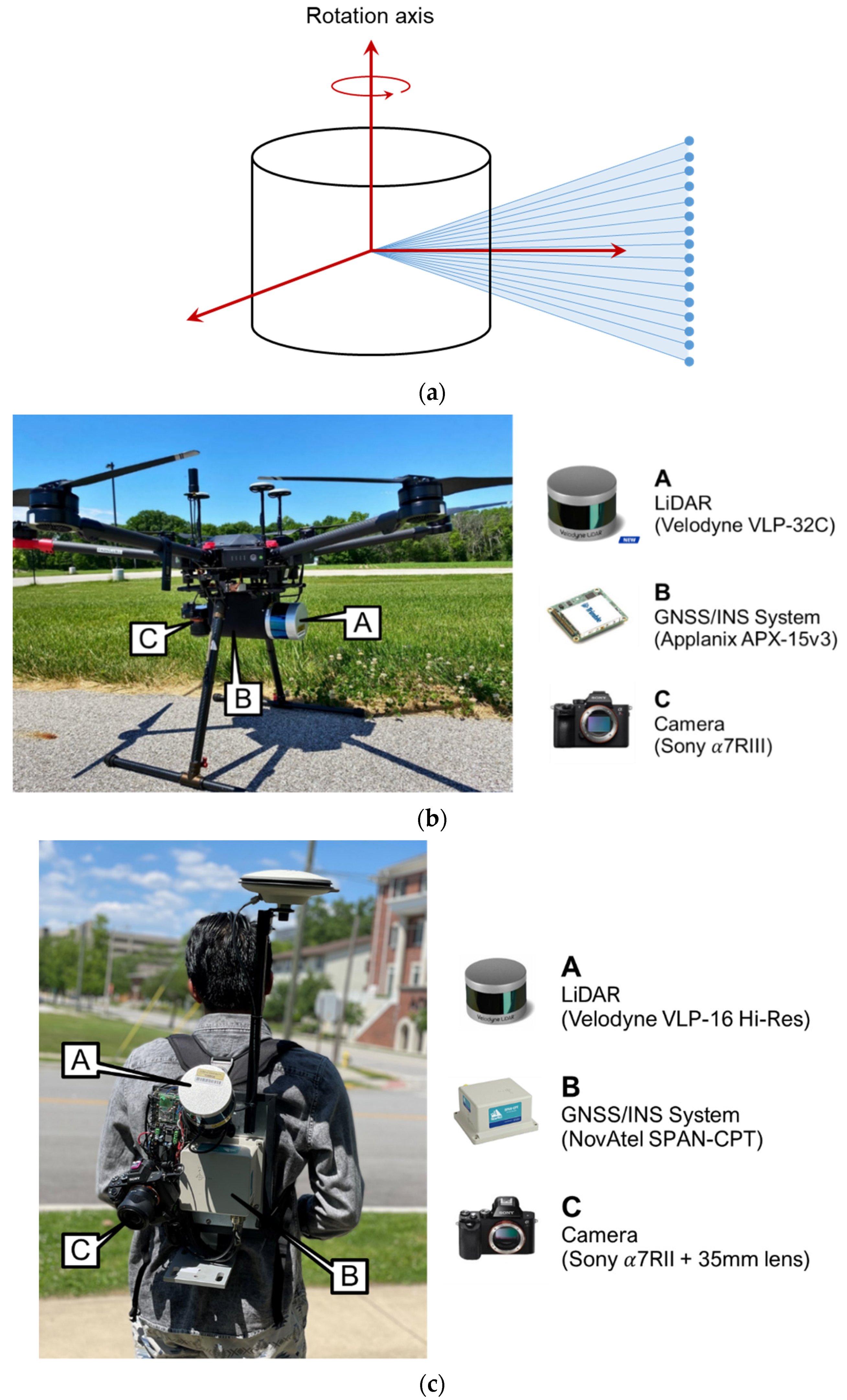
2.1.3. UAV and Backpack Systems

There were two in-house developed mobile LiDAR systems—UAV and Backpack systems (as shown in Figure 2)—used in this study. Both systems are equipped with a multi-beam spinning laser scanner, camera, and GNSS/INS unit for direct georeferencing. Unlike linear LiDAR systems onboard most manned airborne mapping systems, multi-beam spinning laser scanners have several beams that could be radially aligned in a vertical plane. The beams are mechanically rotated around the scanner’s vertical axis to provide a larger area coverage (see Figure 2a). Figure 2b,c show the UAV and Backpack systems, respectively, together with the onboard sensors. The specifications of the LiDAR [39,40] and georeferencing [41,42] units for each system are listed in Table 1. System calibration was conducted using the in-situ calibration procedure proposed by Ravi et al. [43]. The expected accuracy of the point cloud was estimated based on the individual sensor specifications and system calibration accuracy using the LiDAR Error Propagation calculator [44], and the results are reported in Table 1.

2.2. Study Site and Dataset Description
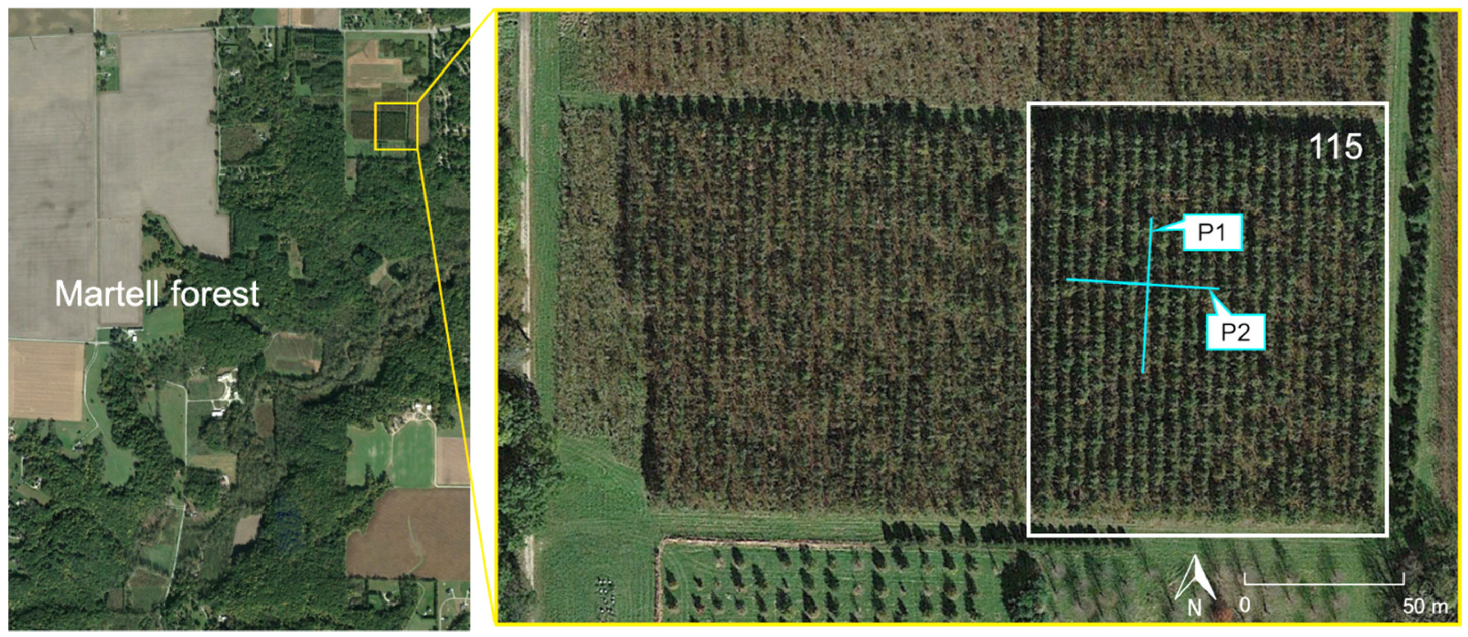
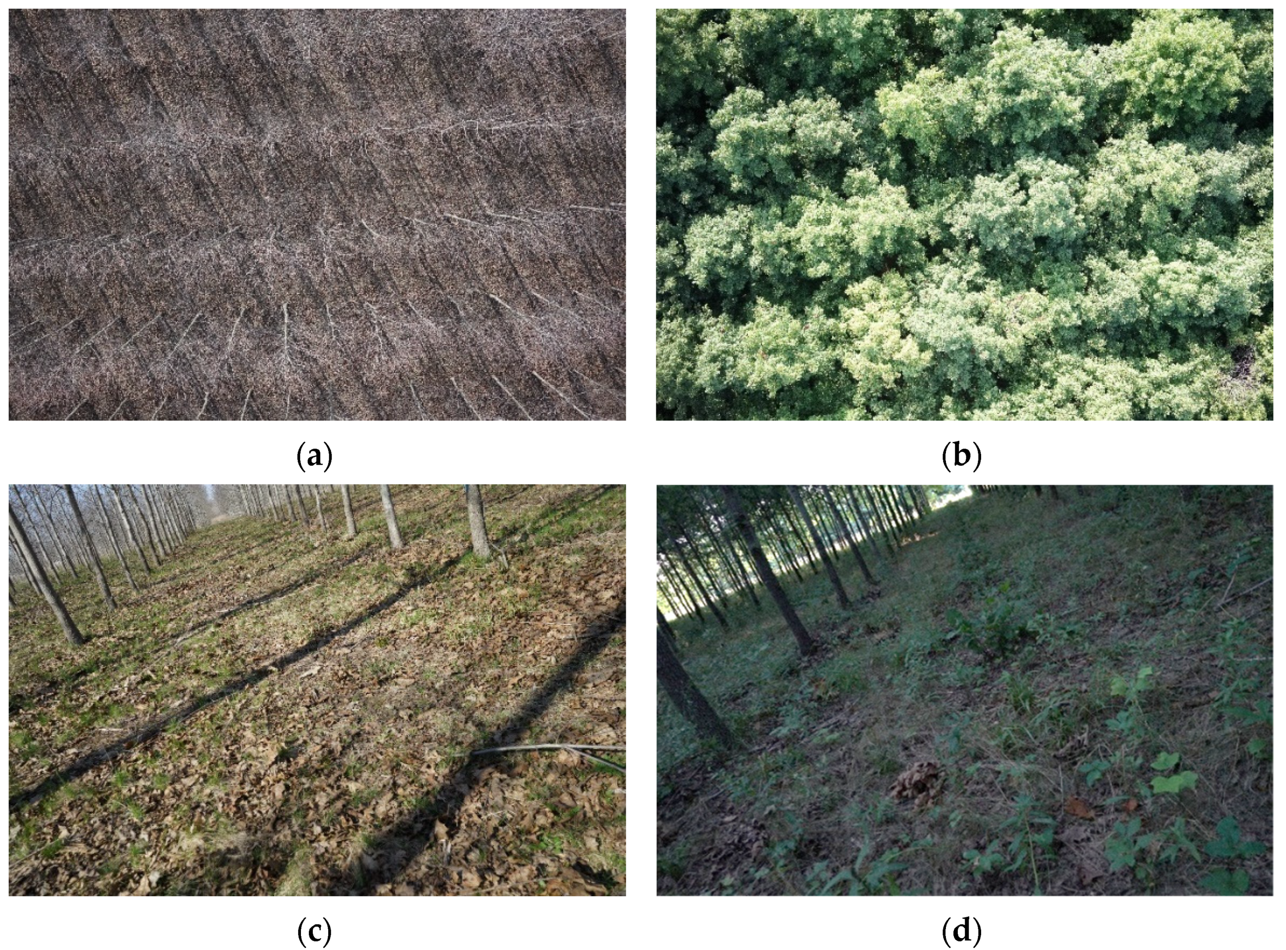
2.2.1. Study Site

LiDAR data were acquired in Martell Forest, a research forest owned and managed by Purdue University, in West Lafayette, Indiana, USA. A forest plantation, Plot 115, as shown in Figure 3, is selected as the study area for this research. The plot was planted in 2007, following a grid pattern: 22 rows with 50 trees per row. Between-row and between-tree spacing values are approximately 5 m and 2.5 m, respectively. Tree height in the plot ranges from 10 to 12 m at measurement year 13 and the average DBH is 12.7 cm. Cross-sectional profiles P1 and P2 are used in the qualitative analysis (as will be discussed later in Section 4.1). Figure 4 displays images captured by the UAV and Backpack systems under leaf-off and leaf-on conditions. The dense foliage and under-canopy vegetation under leaf-on condition can be clearly seen in Figure 4b,d.

2.2.2. USGS Statewide LiDAR Data

Several temporal LiDAR datasets over Martell Forest are publicly available through the USGS 3D elevation program at 3DEP LidarExplorer [45]. The most recent dataset, acquired in spring 2018 under the leaf-off condition, is used for the comparative analysis in this study [46]. According to the metadata, this dataset was acquired using a linear LiDAR system at a height of approximately 2000 m above ground. The data acquisition and processing met the QL2 requirement specified in the USGS LiDAR base specification [47]; namely, better than 10 cm vertical accuracy and nominal pulse spacing less than 70 cm (i.e., nominal pulse density of more than two points per square meter).

2.2.3. VeriDaaS Geiger-Mode LiDAR Data

The Geiger-mode LiDAR dataset was collected and processed independently by VeriDaaS Corporation following the USGS QL1 specifications; namely, better than 10 cm vertical accuracy and nominal pulse spacing less than 35 cm (i.e., nominal pulse density of more than 8 points per square meter). The data were acquired on 3 September 2021 (leaf-on) at a height of approximately 3700 m above ground. Data processing started with an initial refinement via a voxel process to achieve a desired point density of 50 points per square meter in this study. A block adjustment procedure was conducted to spatially reposition the point cloud by aligning points within overlapping flight lines. This block adjustment procedure can improve the point cloud quality by compensating for inherent georeferencing errors from the GNSS/INS system. Post-processed point clouds are expected to have 5 cm accuracy along the vertical direction (i.e., meeting the USGS QL0 specifications).

2.2.4. UAV LiDAR Data

The two datasets were captured by the UAV system: 13 March 2021 (leaf-off) and 2 August 2021 (leaf-on). The UAV was flown at a flying height of 40 m above ground and ground speed of 3.5 m/s, and the lateral distance between neighboring flight lines was 11 m. The point clouds were reconstructed with a 140° field of view (FOV) across the flying direction (±70° from nadir), resulting in a sidelap percentage of about 95%. The large FOV was chosen to mitigate occlusions because an object can be captured by multiple laser beams from different view angles at various times. As has been mentioned in Table 1, the accuracy of derived point clouds is expected to be in the 5 cm to 6 cm range.

2.2.5. Backpack LiDAR Data

The two datasets were acquired using the Backpack system: 1 April 2021 (leaf-off) and 5 August 2021 (leaf-on). The Backpack was carried by an operator while walking under the forest canopy between individual tree rows. The initially derived point clouds from the Backpack system show a misalignment ranging from 0.5 m to 2 m within points from neighboring tracks. This misalignment is attributed to the intermittent access to GNSS signal under forest canopy, which leads to a deterioration in the trajectory quality. To mitigate the negative impact of GNSS signal outage and produce high-precision point clouds, the trajectory enhancement approach, as described in Section 3.1, was applied to the Backpack datasets. The UAV leaf-off dataset was used as a reference in this process, i.e., the Backpack datasets after trajectory enhancement would be aligned with the UAV leaf-off dataset. Following the trajectory enhancement, the accuracy of the Backpack LiDAR data is expected to be in the 3 cm to 4 cm range.

3. Methodology

This section starts with introducing the trajectory enhancement approach that mitigates the impact of GNSS signal outages and improves point cloud quality for the Backpack data. Comprehensive comparative analysis of different datasets was then carried out to evaluate point cloud characteristics and quality as well as the ability to derive various forest inventory metrics. The workflow has three main components: (1) ground filtering and height normalization, (2) point cloud characterization and quality assessment, and (3) forest inventory, as outlined in Figure 5.

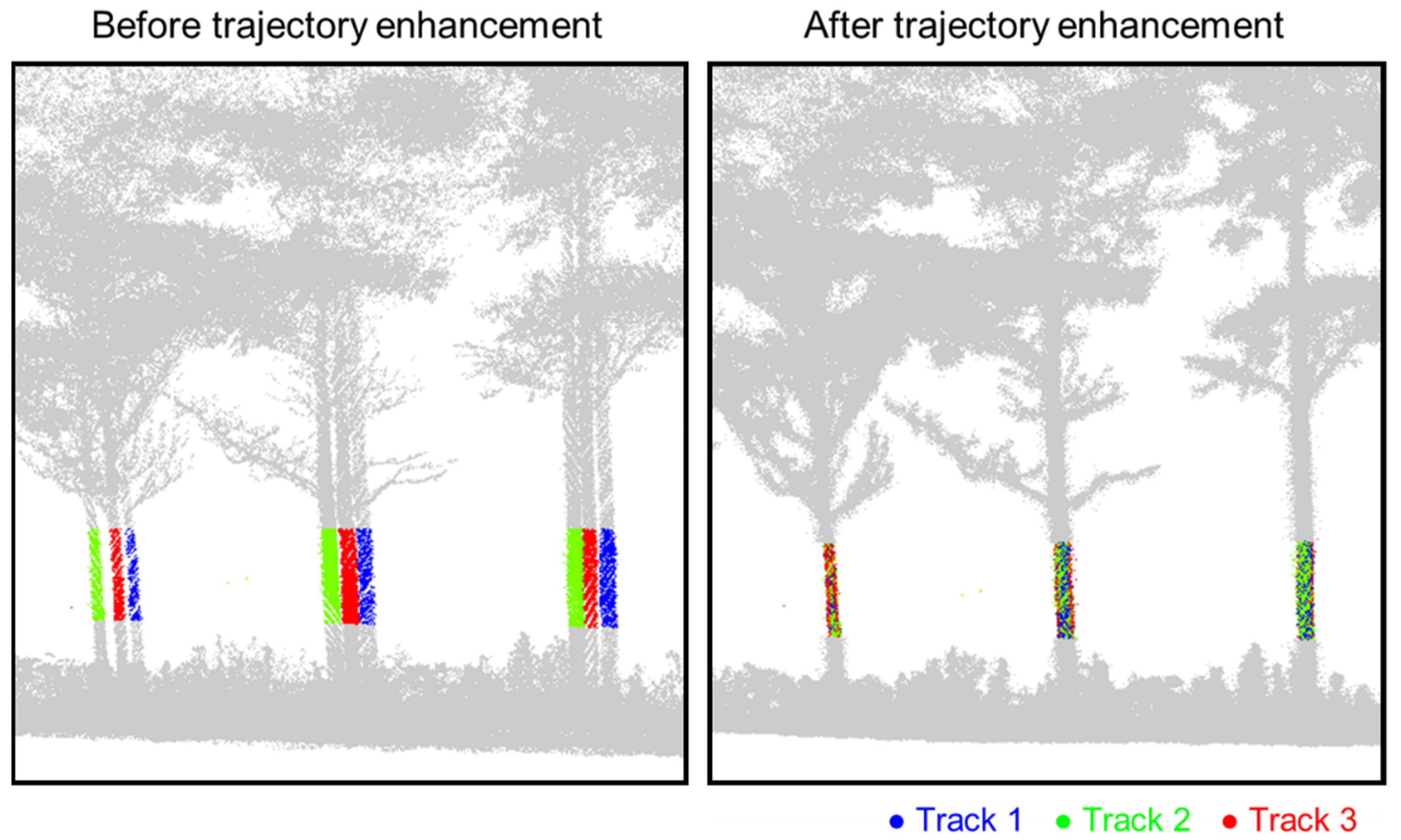
3.1. Trajectory Enhancement for Backpack Data

Point cloud misalignment caused by inaccurate trajectory owing to GNSS signal outages is a major challenge for under-canopy Backpack surveys. This study proposed a novel strategy that enhances the trajectory quality using automatically extracted and matched features from point clouds captured in different tracks (i.e., straight portions of the trajectory). The features used in this study include tree trunks (cylindrical features) and terrain patches (planar features). The conceptual basis of the proposed approach is that any inaccuracy in trajectory parameters would manifest in the point cloud as discrepancies among conjugate features. Therefore, corrections to the trajectory parameters can be estimated by minimizing the normal distance between the LiDAR points and the best-fitted cylinder or plane using least-squares adjustment (LSA).
Assuming that the trajectory is precise, the coordinates of the LiDAR point, I , captured at time, t , in the mapping frame can be written as per Equation (1), which is graphically illustrated in Figure 6. Here, r b ( t ) m and R b ( t ) m are the trajectory position and orientation parameters; r l u b and R l u b are the LiDAR mounting parameters estimated from the system calibration; r I l u ( t ) is the point coordinates in the laser unit frame. The point positioning equation can be expressed symbolically as per Equation (2). For scenarios with GNSS signal outages, corrections to the trajectory parameters are required to precisely reconstruct the LiDAR point. The adjusted coordinates of the LiDAR point, r I m ( a d j u s t e d ) , are expressed symbolically in Equation (3), where δ r b ( t ) m and δ R b ( t ) m are the corrections to the trajectory position and orientation parameters, respectively.
r I m = r b ( t ) m + R b ( t ) m r l u b + R b ( t ) m R l u b r I l u ( t )
r I m = f ( r b ( t ) m ,   R b ( t ) m ,   r l u b ,   R l u b ,   r I l u ( t ) )
r I m ( a d j u s t e d ) = f ( r b ( t ) m ,   R b ( t ) m ,   δ r b ( t ) m ,   δ R b ( t ) m , r l u b ,   R l u b ,   r I l u ( t ) )
The mathematical model of the LSA involves two sets of observation equations. The first set of observation equations (Equation (4)) comes from cylindrical and planar features. The corresponding target function (Equation (5)) minimizes the squared sum of the weighted normal distances between each LiDAR point and its corresponding parametric model, as illustrated in Figure 7. Here, f t k m is the feature parameters for the kth feature; n d ( r I m ( a d j u s t e d ) , f t k m ) denotes the normal distance between the LiDAR point and its corresponding feature; w f t k m is the weight of the feature parameters, which is assigned based on the expected accuracy of the feature. The second set of observation equations (Equation (6)) incorporates prior information from the trajectory. The corresponding target function (Equation (7)) ensures that the corrections to the trajectory parameters are estimated while considering the initial accuracy of the respective parameters reported by the GNSS/INS post-processing software. Here, the weight w r b ( t ) m and w R b ( t ) m are assigned based on the standard deviation of the respective trajectory parameters. One thing to note is that the proposed approach essentially solves the corrections to the trajectory parameters, and is therefore more applicable as compared to previous work that assumes a rigid body transformation between tracks [48]. Figure 8 presents a sample trajectory enhancement result. The initial misalignment between tracks that results in different versions of the tree trunks is eliminated after trajectory enhancement.
n d ( r I m ( a d j u s t e d ) , f t k m ) = 0
argmin δ r b ( t ) m ,   δ R b ( t ) m , f t k m       points   and   features ( n d ( r I m ( a d j u s t e d ) , f t k m ) ) 2 w f t k m
r b ( t ) m ( a d j u s t e d ) = r b ( t ) m + δ r b ( t ) m R b ( t ) m ( a d j u s t e d ) = R b ( t ) m δ R b ( t ) m
argmin δ r b ( t ) m       trajectory   points ( δ r b ( t ) m ) 2 w r b ( t ) m argmin δ R b ( t ) m       trajectory   points ( δ R b ( t ) m ) 2 w R b ( t ) m

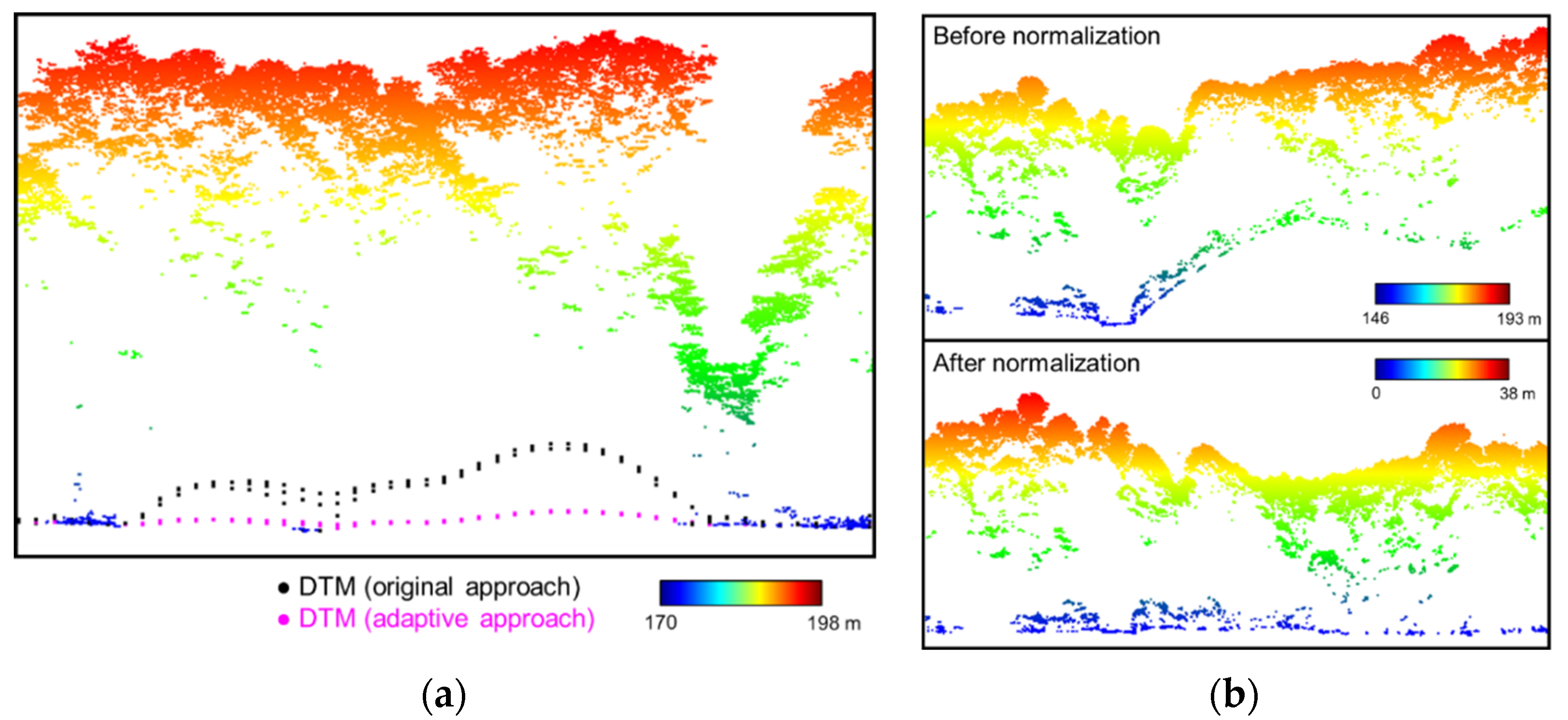
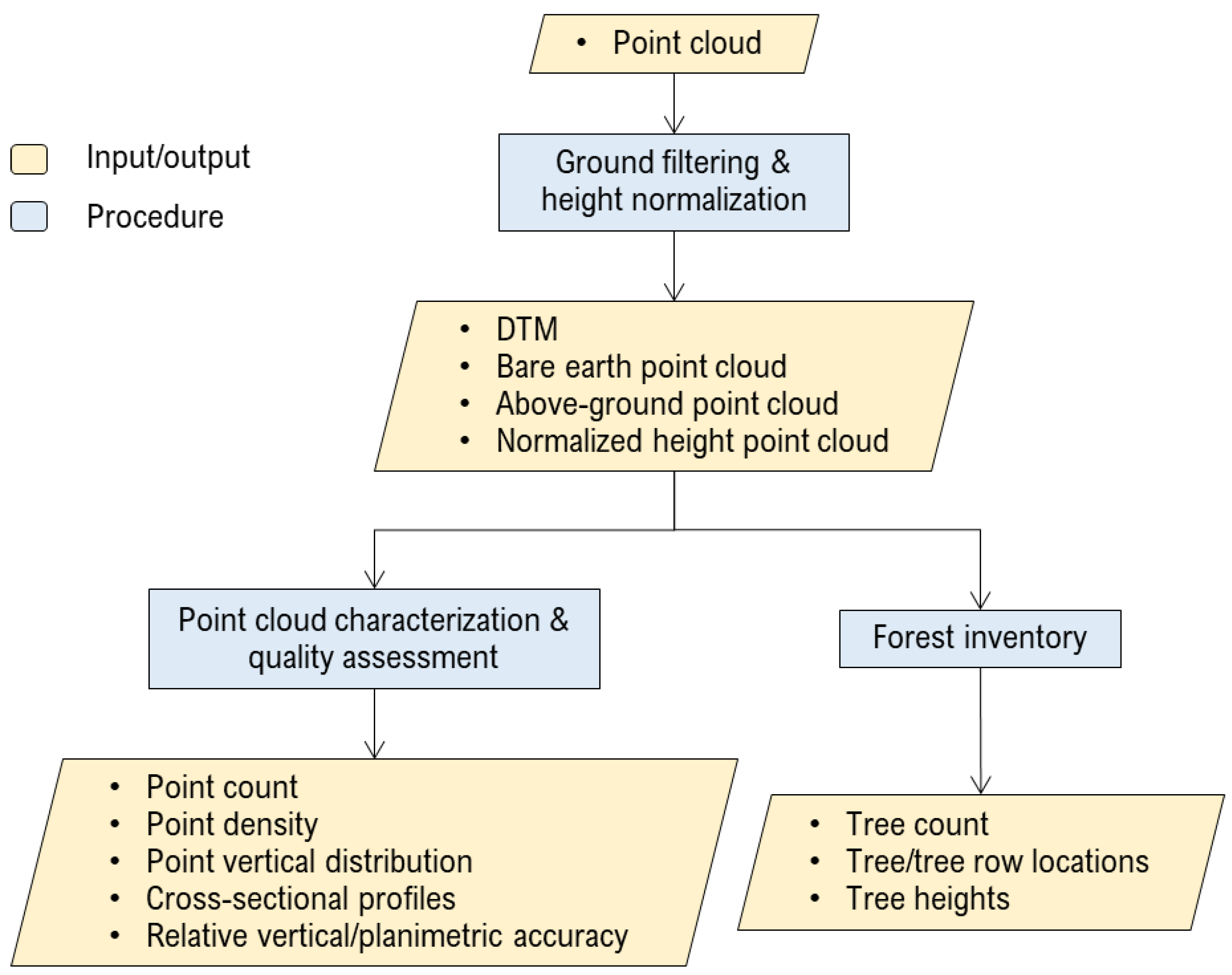
3.2. Ground Filtering and Height Normalization

Prior to the comparative analysis, a ground filtering algorithm, the adaptive cloth simulation [49], is applied to generate a DTM and separate ground points from the above-ground points. The original cloth simulation strategy uses a cloth, with pre-defined homogeneous rigidity, which is draped on top of an inverted point cloud to generate a DTM and isolate ground points [50]. To mitigate the impact of uneven, sparse point cloud distribution along the lower canopy, which is the case for captured aerial LiDAR data under leaf-on conditions, the adaptive approach redefines the cloth rigidity based on the derived bare earth from the original cloth simulation approach [49]. The DTM is then used to normalize the point cloud so that its height would be relative to the ground level. Figure 9 shows sample ground filtering and height normalization results using the VeriDaaS dataset. A closer inspection of Figure 9a reveals that the adaptive cloth simulation approach provides a more realistic representation of the terrain model. However, a slight increase in the elevation of the generated terrain model is inevitable, given the sparse nature of the ground points. In Figure 9b, the elevation values before and after normalization are the ellipsoidal height (relative to a reference ellipsoid that approximates the Earth surface) and height above ground, respectively.

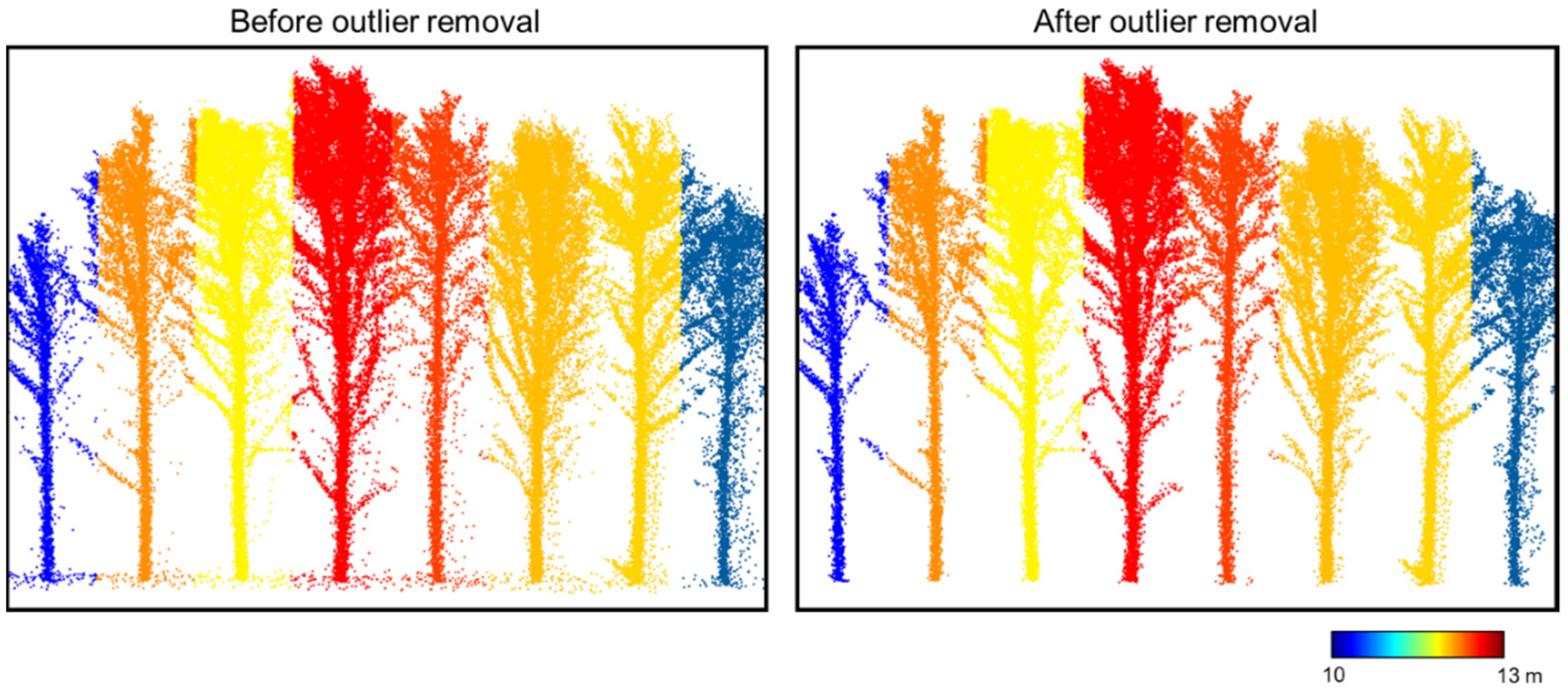
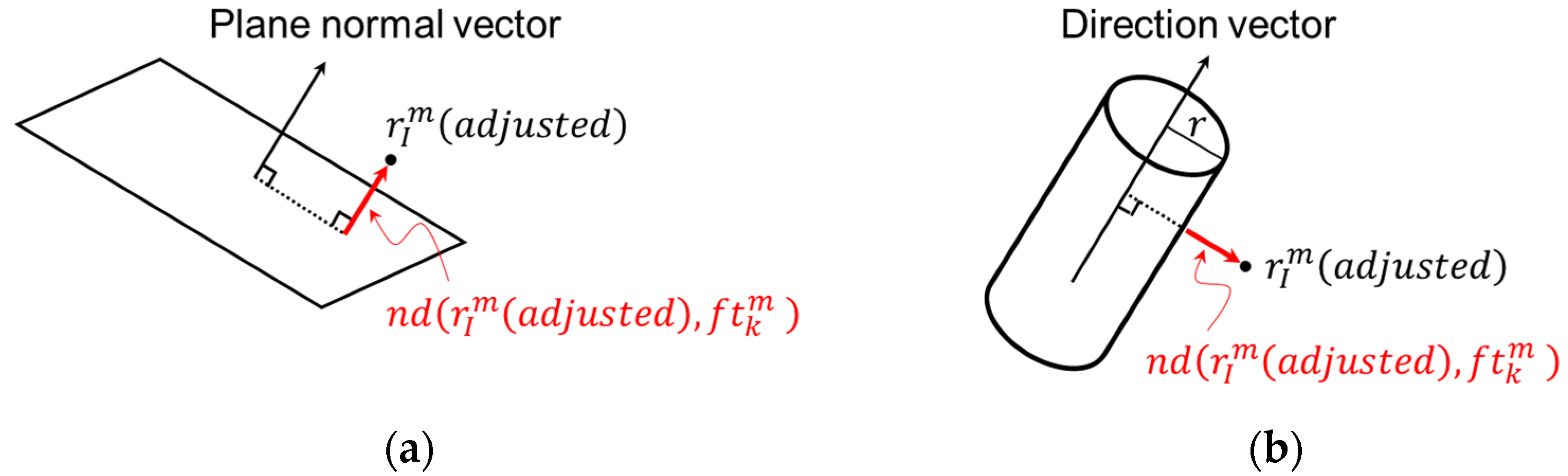
3.3. Point Cloud Characterization and Quality Assessment

The comparative analysis starts with investigating the distribution within the acquired point clouds from different systems. First, the numbers of points in the entire, bare earth, and above-ground point clouds within the study area captured by each system are listed. Next, planimetric point density (point per square meter, ppsm) over the study area is reported for both the entire point cloud as well as ground points, providing another indication of the amount of information captured by different systems along the terrain and canopy. The point distribution along the vertical direction is quantified using a histogram, showing the number of points at different elevations. Cross-sectional profiles are extracted from the point clouds to examine the overall representation of tree structure and alignment between different datasets.
Quantitative assessment of the relative accuracy between different datasets is conducted using the feature-based approach described Lin and Habib [51] and Lin et al. [14], where estimates of the relative vertical and planimetric accuracy are established using terrain patches, and tree and tree row locations, respectively. For the relative vertical accuracy assessment, separation between extracted terrain patches from different datasets along their surface normal direction are evaluated. In addition, a histogram of the elevation differences between conjugate DTM cells is presented to illustrate the nature of agreement between terrain models derived from different datasets. For planimetric accuracy, horizontal shifts between derived tree or tree row locations from different datasets are reported.

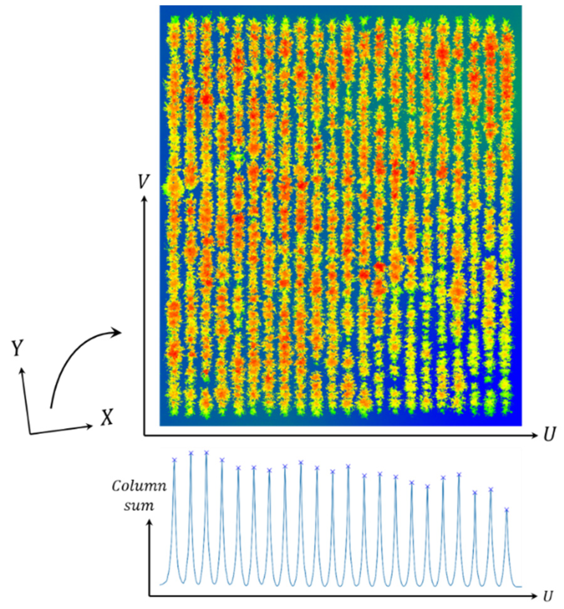
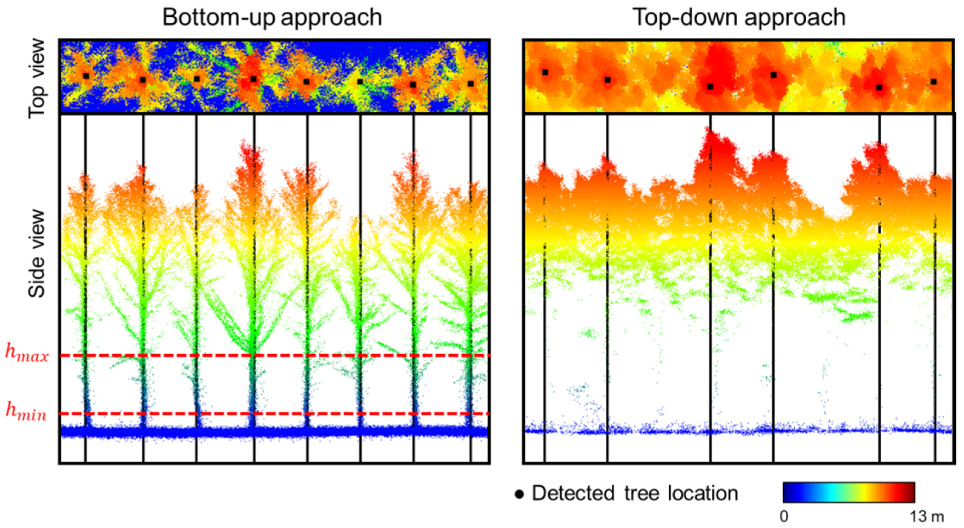
3.4. Forest Inventory

Having verified the point cloud quality, individual tree and tree row locations are identified using the peak detection-based approach outlined in Lin and Habib [51] and Lin et al. [14]. The conceptual basis of this approach is that higher point density and higher elevation correspond to tree or tree row locations. For plantations, tree rows are represented as 2D lines along the XY plane, assuming they are planted along straight lines. Tree row localization starts with rotating the normalized height point cloud to a local coordinate system (UV) so that tree rows are along the V axis, as shown in Figure 10. Next, 2D cells along the UV plane are created and tree row locations are identified by detecting local peaks of the column sum of the metric—the sum of elevations of all points in a cell. Unlike tree rows, trees are represented as 2D points along the XY plane. Depending on whether tree trunks are visible in the point cloud, a bottom-up or top-down strategy is adopted for tree localization, as illustrated in Figure 11. The bottom-up strategy detects tree trunks by evaluating point density and elevation distribution of the lower canopy. User-defined minimum and maximum height thresholds ( h m a x and h m i n ) are applied to the normalized height point cloud to extract segments that roughly correspond to the trunks. The metric used for peak detection is the sum of elevations of all points in a cell. The top-down strategy, on the other hand, identifies tree locations by finding local maxima in the normalized height point cloud. The 90th percentile elevation of each cell is evaluated and used as the metric for peak detection. As can be seen in Figure 11, the top-down approach is more likely to miss small trees.
Tree heights are estimated using the detected tree locations and normalized height above-ground point cloud. For reliable height estimation, a statistical outlier removal strategy [52] is applied to the point cloud to filter scattered points. The algorithm first computes the mean and standard deviation of the distances between each point to its k nearest neighbors. It then trims points which fall outside the average distance plus a user-defined multiplication factor times the standard deviation. Next, neighboring points within a 2D search radius for each tree location are identified and the highest elevation among these points is used to represent the tree height. An example of outlier removal and tree height estimation is shown in Figure 12.

4. Experimental Results

This section presents the experimental results of the comparative analysis, including point cloud characteristics, quality assessment, and forest inventory metrics. The six datasets acquired from different LiDAR systems, hereafter denoted as the USGS-3DEP, VeriDaaS, UAV leaf-on, UAV leaf-off, Backpack leaf-on, and Backpack leaf-off datasets, were used for the experiments.

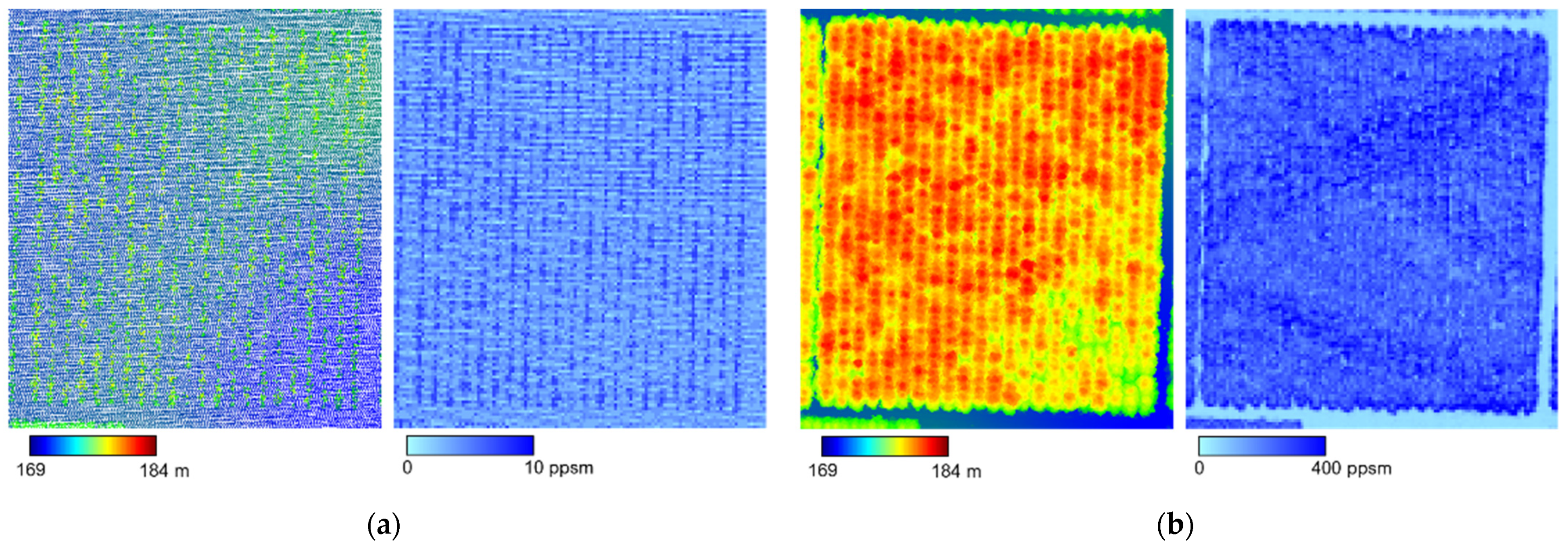
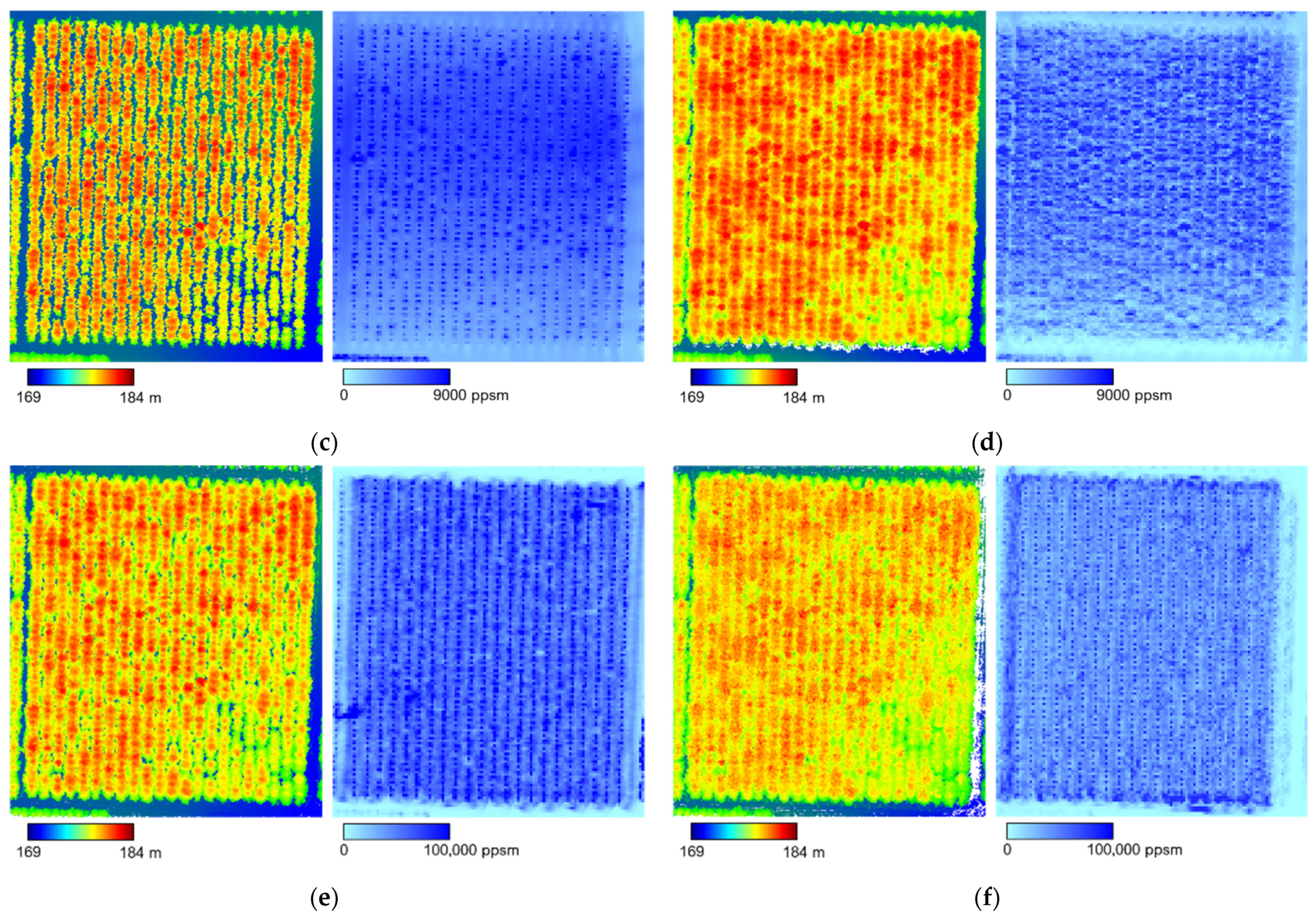
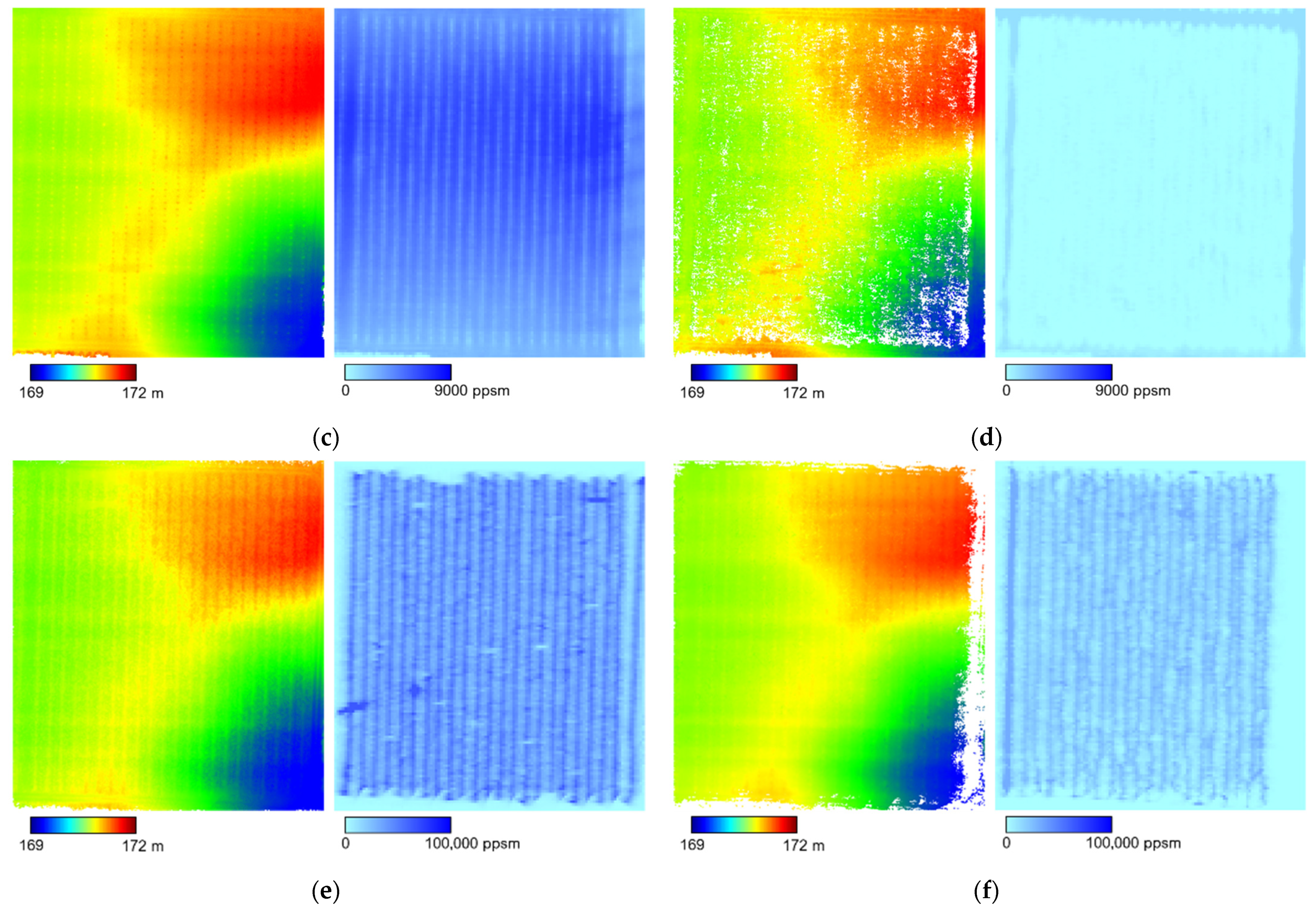
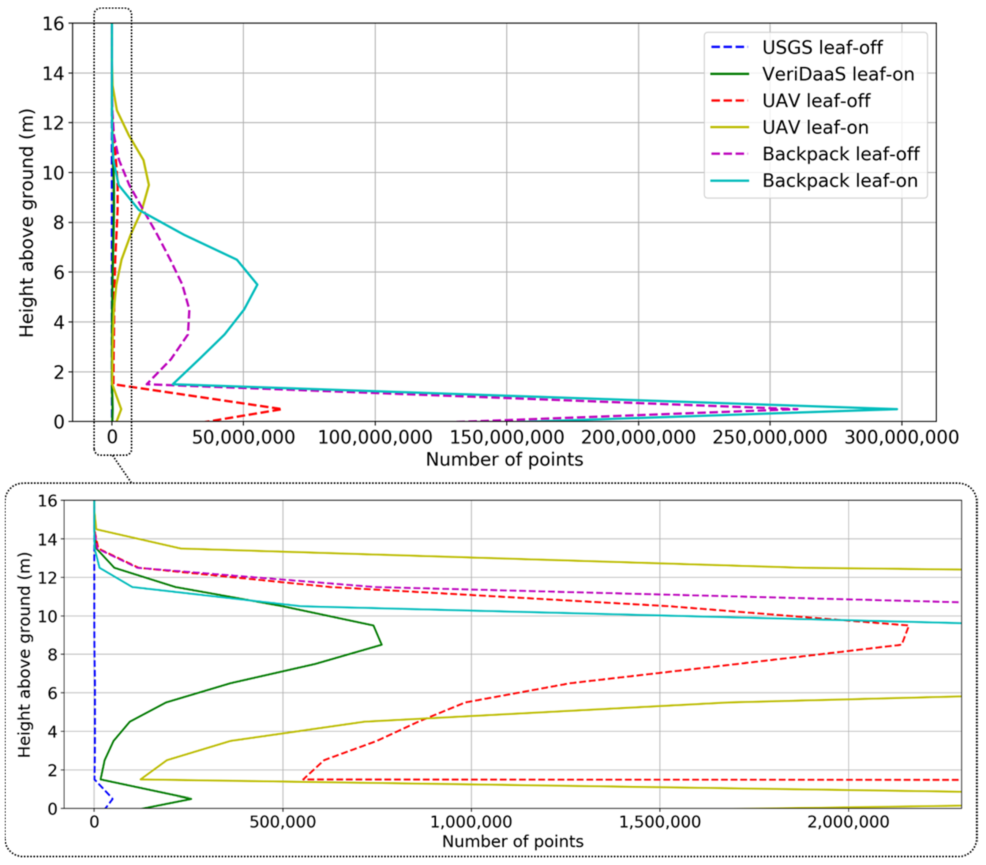
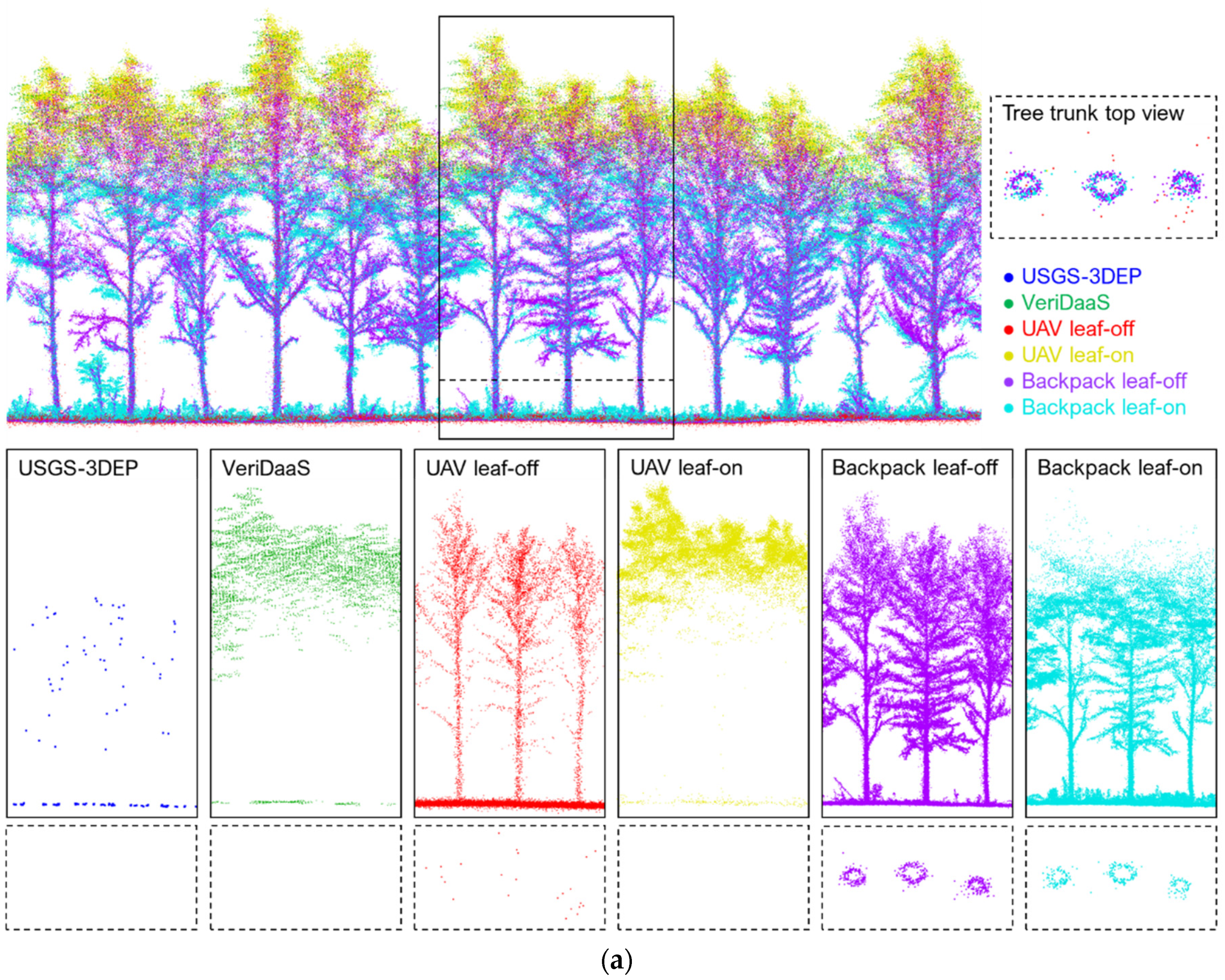
4.1. Point Cloud Characteristics

A thorough investigation of the level of information acquired by multi-platform, multi-resolution, and multi-temporal datasets forms the basis of understanding the capability and limitations of different LiDAR systems and the potential to derive forest inventory metrics at various scales. Point cloud covering Plot 115 in the forest plantation was extracted from each dataset. The adaptive cloth simulation algorithm was then applied to separate ground and above-ground points and generate DTMs at 1 m resolution (the 1 m cell size is chosen to accommodate the sparse nature of the USGS-3DEP data). The height of the point cloud was then normalized by subtracting the terrain elevation.
The number of points captured by the USGS-3DEP, VeriDaaS, UAV leaf-on, UAV leaf-off, Backpack leaf-on, and Backpack leaf-off datasets and the percentage of ground and above-ground points are reported in Table 2. The huge variation in number of points can be clearly seen—the proximal Backpack system acquired roughly 15,000 times more points than the aerial linear system (873 million for the Backpack leaf-off datasets vs. 0.06 million for the USGS-3DEP dataset). The number of points captured by the Geiger-mode LiDAR (3 million for the VeriDaaS dataset) is around 50 times more than that captured by the traditional linear LiDAR (0.06 million for the USGS-3DEP dataset). For the aerial systems (linear, Geiger-mode, and UAV LiDAR), canopy cover has a critical impact on the LiDAR penetration, resulting in a striking contrast in ground point percentage between leaf-on and leaf-off datasets. The proximal Backpack system has a more balanced ground and above-ground point distribution under different canopy cover conditions.
To gain insight into planimetric point distribution, Figure 13 and Figure 14 visualize the entire and bare earth point clouds before height normalization (colored by ellipsoidal height), respectively, along with the corresponding point density maps (with 1 m cell size). The 25th percentile, median, and 75th percentile of the point density of the entire and bare earth point clouds for each dataset are reported in Table 3. Looking into the entire point clouds, the five datasets acquired during 2021 (Figure 13b–f) show similar altitudes ranging from 169 m to 184 m. The foliage growth can be observed in the leaf-on datasets (Figure 13b,d,f). The USGS-3DEP dataset (Figure 13a) displays a lower altitude (the maximum altitude in this dataset is about 181 m) because it was collected four years prior to other datasets, and thus the trees are shorter. For the entire point clouds, the point density maps reveal obvious dissimilarity between data from different systems. The Backpack LiDAR provides the highest point density, followed by the UAV LiDAR, Geiger-mode LiDAR, and linear LiDAR. Examining the bare earth provides an understanding of the ability of the LiDAR systems to penetrate through vegetation and capture the terrain under different canopy cover scenarios. In Figure 14, the bare earth point clouds from the six datasets exhibit a comparable spatial pattern. This finding suggests that all the systems were able to capture some ground points, which can be reliably extracted using the adaptive cloth simulation algorithm. It also indicates that the terrain elevation remains stable regardless of which LiDAR dataset was used. The relative low point density together with observable gaps in the point clouds under leaf-on condition, in particular for the aerial systems (see Figure 14b,d and Table 3), reveal the limited LiDAR penetration under the dense canopy. In contrast, owing to the leaf-off condition during data acquisition, the ground points from the USGS-3DEP dataset have a uniform spatial distribution even though the point density is the lowest.
The vertical point distribution is examined using a histogram of the number of points at different heights above ground for the entire point clouds, as shown in Figure 15. Regardless of the clear disparity in the number of points, the peaks around the height of 0 m above ground for all datasets indicate that all the systems were able to capture a considerable number of ground points. The above-ground points from the USGS-3DEP dataset are extremely sparse. The UAV leaf-off dataset captures a reasonable number of points from top to lower-middle of the canopy. The leaf-on datasets from the aerial systems (VeriDaaS and UAV) attain their peaks in the upper canopy and the numbers of points drop significantly in the lower-middle canopy comprising the tree trunks. For the Backpack leaf-off and leaf-on datasets, the majority of the above-ground points captures the lower-middle canopy. The dense foliage under the leaf-on condition limits the amount of Backpack LiDAR penetration, leading to the obvious decline in the number of points in the top canopy area (over 11 m above ground).
The two cross-sectional profiles, P1 (along tree rows) and P2 (across tree rows), whose locations are shown in Figure 3, were extracted to investigate the level of detail captured by different systems as well as the point cloud alignment. Figure 16 shows the side view of the two profiles. The combined point clouds (Figure 16a,b—top) depict the alignment quality. Because the tree rows in the plantation are mainly along the Y direction, the profiles along (P1) and across (P2) tree rows would provide information to assess the point cloud alignment along the X/Z and Y/Z directions, respectively. In general, profiles from different datasets exhibit good overall alignment in all directions. The individual point clouds (Figure 16a,b—bottom) provide a glimpse of the level of information captured. The USGS-3DEP dataset, despite being extremely sparse, provides adequate information for terrain representation and tree height estimation. However, such sparse information is not adequate to describe tree structure. Both the VeriDaaS and UAV leaf-on datasets capture the upper canopy and terrain in spite of the latter having a much higher point density and better degree of penetration. The lower-middle canopy portion is barely captured for the leaf-on datasets due to the heavy foliage that inhibits the aerial LiDAR penetration. Under the leaf-off condition, the UAV obtained information from the canopy top all the way to the ground, where individual trees can be clearly identified from the point cloud. However, the precision and level of detail from the UAV-based point clouds are not comparable to those from the Backpack system. Point clouds from the Backpack have the best point density and precision among all the datasets, as can be seen by the better definition of tree trunks and structures. The Backpack leaf-off dataset has a more balanced vertical distribution whereas the leaf-on dataset acquires negligible points near the top canopy due to the limited LiDAR penetration.

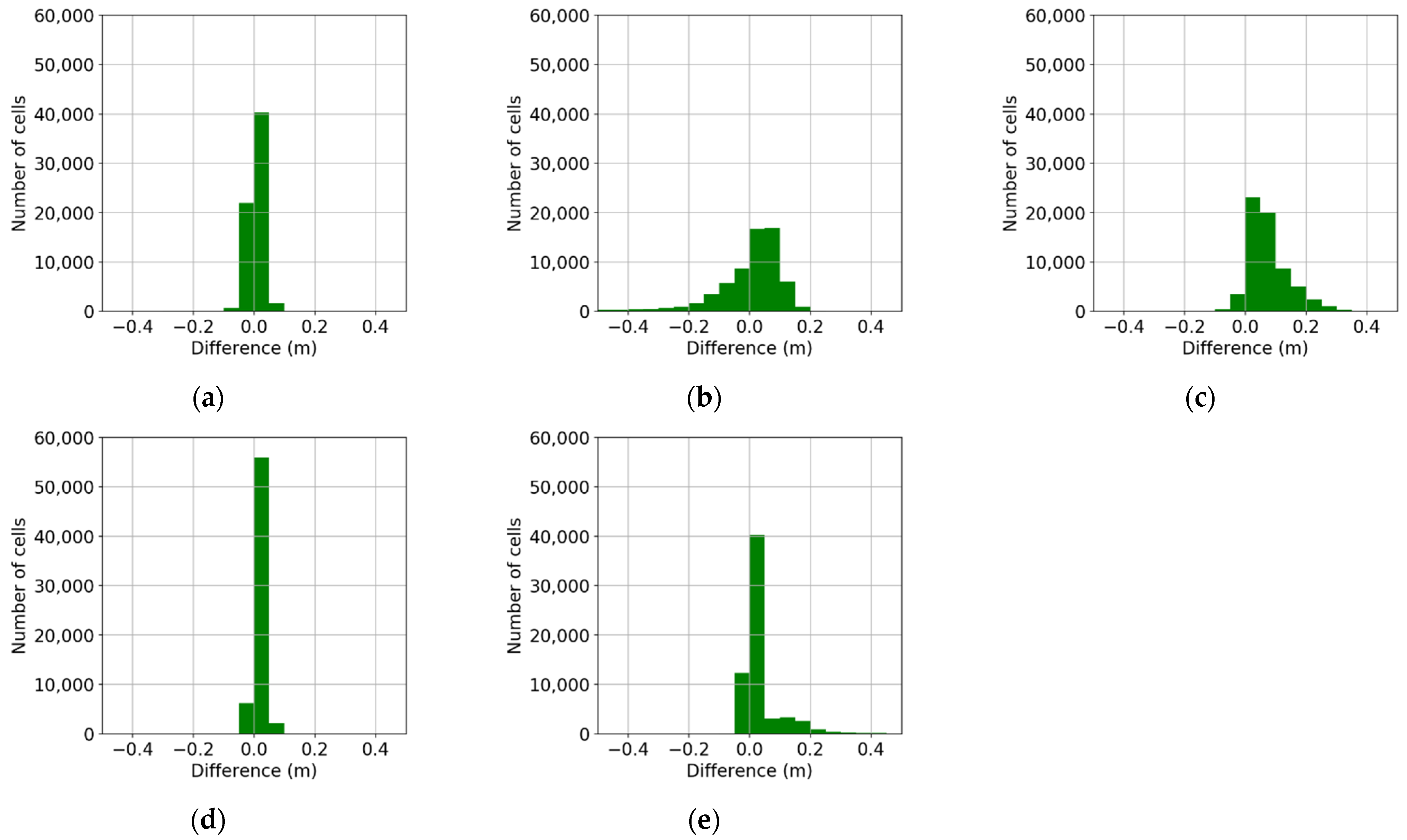
4.2. Quantitative Assessment of Relative Data Quality

In this section, the alignment between multi-platform, multi-resolution, and multi-temporal datasets was evaluated quantitatively using features that can be automatically identified from the plantation. The relative accuracy is assessed between two point clouds at a time, using the UAV datasets as references. The USGS-3DEP and VeriDaaS datasets were compared against UAV leaf-off and leaf-on datasets, respectively, because they were acquired under similar canopy cover scenarios. The comparison between the two UAV datasets would be an indication of any changes in the plantation between leaf-off and leaf-on conditions. The Backpack leaf-off and leaf-on datasets were compared against the UAV leaf-off dataset because the latter served as the reference for trajectory enhancement. To summarize, the relative quality between point clouds listed below are reported in this section (A through E will be used as identifiers for these comparison pairs):
  • UAV leaf-off vs. USGS-3DEP (leaf-off) datasets;
  • UAV leaf-on vs. VeriDaaS (leaf-on) datasets;
  • UAV leaf-off vs. UAV leaf-on datasets;
  • UAV leaf-off vs. Backpack leaf-off datasets;
  • UAV leaf-off vs. Backpack leaf-on datasets.
The relative vertical discrepancy was evaluated using terrain patches extracted from the bare earth point clouds. The terrain patches are planar features with normal vectors mainly along the Z direction, and thus provide information for vertical discrepancy estimation. Table 4 reports the square root of a posteriori variance factor ( σ 0 ^ ), an indication of the noise level of the point clouds, and estimated vertical shift ( d z ). The discrepancy estimation between UAV leaf-off and UAV leaf-on datasets suggests an 8 cm shift, which could be attributed to the growth of under-canopy vegetation (see Figure 4d). The estimated discrepancies between other datasets reveal that point clouds under similar canopy cover scenarios are in good agreement within a ±3 cm range along the vertical direction.
The elevations difference between DTMs derived from different datasets are also visualized using histograms, as shown in Figure 17, depicting the relative accuracy of the terrain models. The median of the elevation difference for Group A, B, C, D, and E is 0.008 m, 0.028 m, 0.059 m, 0.018 m, and 0.015 m, respectively. The slightly larger difference between DTMs from the VeriDaaS and UAV leaf-on datasets (Figure 17b) is mainly attributed to the sparse ground points in the VeriDaaS dataset that lead to artifacts in the DTM generation process. As mentioned earlier, the adaptive cloth simulation still produces terrain with slightly higher elevation when dealing with extremely sparse points. The positive bias between the UAV leaf-off and leaf-on datasets (Figure 17c) reveals the impact of understory vegetation growth. Overall, DTMs derived from all datasets are of comparable accuracy irrespective of point density and canopy cover conditions.
The relative planimetric discrepancy was evaluated using tree row and individual tree locations. In this study, tree rows are linear features whose line directions are mainly along the Y direction, and thus provide discrepancy information for estimating the X shift. Table 5 reports the square root of a posteriori variance factor ( σ 0 ^ ) and the estimated X shift ( d x ) using tree row locations. Tree locations, on the other hand, are 2D points that can be used to evaluate the X and Y shifts. The square root of a posteriori variance factor ( σ 0 ^ ) and the estimated X and Y shifts ( d x and d y ) using tree locations are shown in Table 6. The point cloud from the USGS-3DEP dataset is adequate for tree row detection, yet too sparse for distinguishing individual trees. Therefore, the USGS-3DEP dataset is not included in the planimetric discrepancy estimation using tree locations. According to the tables, Group A, C, D, and E suggest point clouds from different datasets are compatible within a ±7 cm range along the planimetric directions, irrespective of the canopy cover conditions. Although Group B shows a larger X discrepancy, it should be noted that the tree row and tree detection under leaf-on condition is less accurate because tree trunks were not captured in the point clouds. Therefore, it is believed that the relative planimetric accuracy between different datasets is in a ±7 cm range (once again, this is reflective of the tree and tree row detection strategies rather than the actual quality of the point clouds).

4.3. Forest Inventory Metrics

In this section, forest inventory metrics, including individual tree counts, tree locations, and tree heights, were derived from the multi-platform, multi-resolution, and multi-temporal datasets. Individual tree locations in the forest plantation were identified using either a top-down or bottom-up peak detection approach. The USGS-3DEP dataset was not included in this analysis because the point cloud was too sparse to capture individual trees. The bottom-up approach was adopted for the UAV leaf-off, Backpack leaf-off, and Backpack leaf-on datasets whereas the top-down approach was used for the VeriDaaS and UAV leaf-on datasets. The cell size for evaluating the metrics for peak detection was set to 10 cm. The performance of tree detection from different datasets was evaluated against manually digitized reference data and the precision, recall, and F1-score are reported in Table 7. In the table, the number of true positives indicates the tree counts detected from each dataset. The datasets that utilized the bottom-up approach all achieve an F1-score higher than 0.90. The slightly worse performance for the Backpack leaf-on dataset is mainly related to the understory plant growth and dense foliage. The datasets that adopted the top-down approach yield a lower performance (F1-score lower than 0.8). The recall rate of around 0.7 in the top-down approach is substantially lower as compared to the bottom-up approach. This is reasonable because the top-down approach is essentially finding the local maxima (based on the normalized height) within the point cloud and thus it is less effective in detecting small trees (see Figure 11).
Individual tree heights were estimated based on the detected tree locations from the UAV leaf-off dataset (1056 trees) using the normalized height point clouds from different datasets. The radius for defining a local neighborhood for each tree location was set to 0.5 m. Table 8 reports the mean, standard deviation, and root-mean-square error (RMSE) of the difference between tree heights from different datasets. According to the table, tree height estimation based on the datasets acquired over a similar period (Groups B and D in Table 8) are in good agreement with an RMSE smaller than 0.3 m. The difference of −4.95 m between tree height estimation from the USGS-3DEP and UAV leaf-off datasets could be a result of tree growth over time because the former was collected during 2018 whereas the latter was acquired in 2021. The increased height of 0.48 m between the UAV leaf-off and leaf-on datasets could be attributed to tree growth as well as additional height due to the foliage in the leaf-on condition. The Backpack leaf-on dataset consistently underestimates the tree height (−0.33 m as compared to the estimation from the UAV leaf-off dataset) because the dense foliage restricts the LiDAR penetration to reach the treetops.

5. Discussion

Comparative analysis of multi-platform, multi-resolution, and multi-temporal LiDAR data is critical because it provides guidelines for selecting appropriate LiDAR systems and data processing tools for different research questions. Although several previous studies have compared different LiDAR systems [20,24,26,27,28,29,30,31], this study presents a more comprehensive investigation of data from linear LiDAR (leaf-off), Geiger-mode LiDAR (leaf-on), UAV multi-beam LiDAR (leaf-off and leaf-on), and Backpack multi-beam LiDAR (leaf-off and leaf-on). Qualitative and quantitative evaluations were conducted to determine the point cloud quality and level of information for forest inventory at various scales.
The investigation of point cloud characteristics shows that Backpack multi-beam LiDAR provides the highest point count and point density, followed by UAV multi-beam LiDAR, airborne Geiger-mode LiDAR, and airborne linear LiDAR. Despite the stark contrast in point density, all the systems provide adequate ground points (irrespective of the canopy cover conditions) from which DTMs could be reliably derived. In terms of point vertical distribution, the aerial and terrestrial systems provide more information of the upper and lower canopy, respectively, due to their different view angles—this observation is consistent with previous research findings [20,26]. The dense canopy would restrict LiDAR penetration and result in a low point percentage on the ground and lower canopy for the aerial systems, and upper canopy for the terrestrial system. Yu et al. [24] reported that the Geiger-mode LiDAR provides denser point clouds while operating at a higher altitude as compared to the conventional linear LiDAR. This study further shows that the Geiger-mode LiDAR can capture similar information as compared to UAV with a lower point density and degree of penetration. The relative accuracy assessment results suggest that the multi-platform, multi-resolution, and multi-temporal datasets are in agreement within a ±3 cm and ±7 cm range along the vertical and planimetric directions, respectively. Precise point cloud alignment provides the foundation of multi-platform, multi-resolution data fusion as well as change detection and forest monitoring using multi-temporal datasets.
Forest inventory metrics including tree locations and tree heights are derived from different datasets. The results suggest that all the systems can be utilized for tree and canopy height estimation. The Geiger-mode LiDAR, UAV LiDAR, and Backpack LiDAR capture adequate information for individual tree identification. The bottom-up tree detection approach achieves better performance as compared to the top-down strategy; however, it requires the tree trunks to be captured in the point cloud. In general, data acquisition under a leaf-off condition is favorable because it results in a more uniform vertical distribution of the point cloud that can better capture forest vertical structure. The qualitative analysis shown in Figure 16 reveals that only the Backpack LiDAR provides high precision point clouds that allow for direct measurements of DBH. For the aerial systems, DBH can be inferred based on other forest inventory metrics such as crown size.
The emerging Geiger-mode LiDAR is compared against traditional linear LiDAR to assess its capability of mapping forest environments. The main findings are as follows:
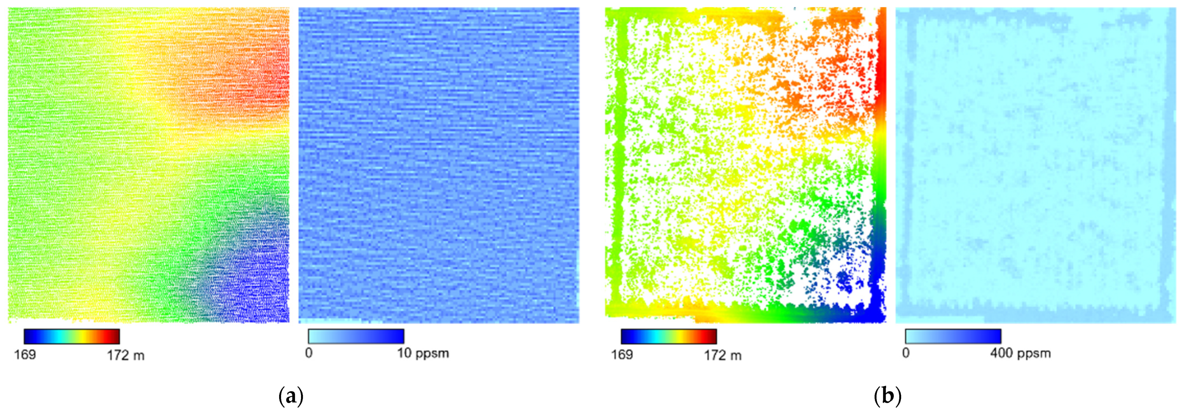
  • The Geiger-mode LiDAR provides denser point clouds while operating at a higher altitude. In this study, the median of the planimetric point density for Geiger-mode and linear LiDAR datasets is 248 ppsm and 4 ppsm, respectively. The flying height of the Geiger-mode and linear LiDAR systems is approximately 3700 m and 2000 m above ground, respectively.
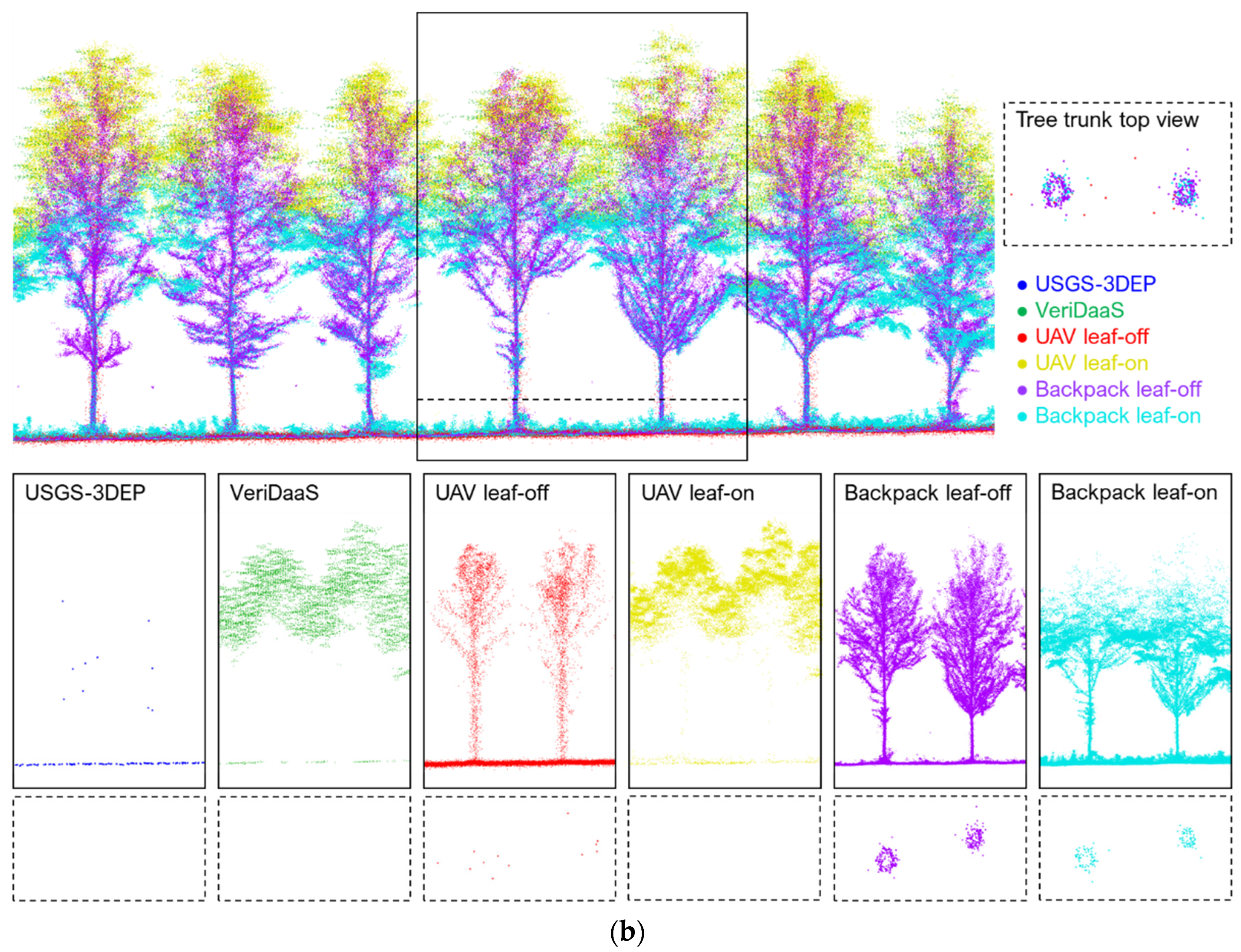
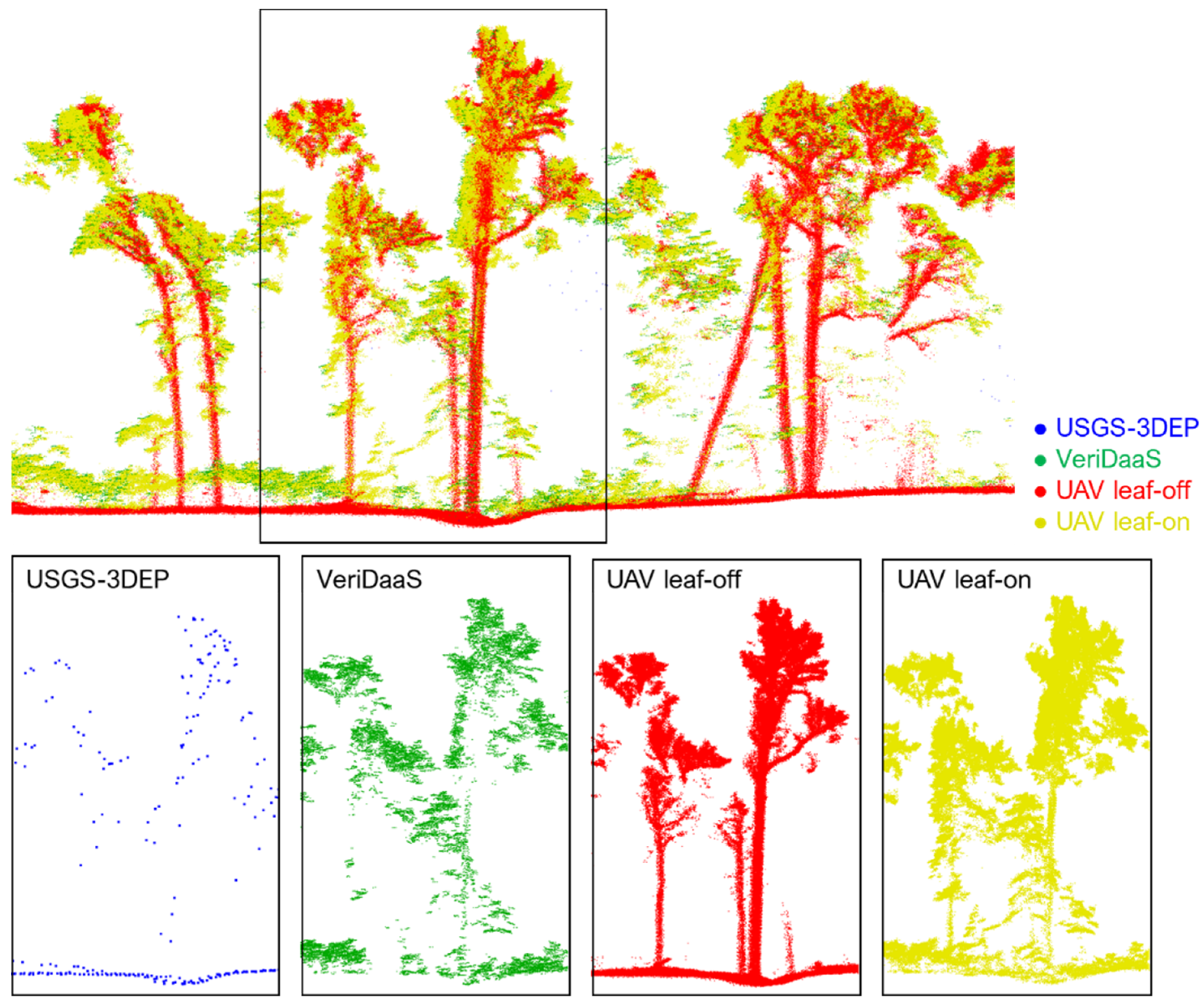
  • The Geiger-mode LiDAR captures a much higher level of information as compared to linear LiDAR. In fact, the level of information obtained by the Geiger-mode LiDAR is found to be close to that captured by the UAV LiDAR (refer to Figure 16).
  • Both the Geiger-mode and linear LiDAR effectively characterize the terrain in the study site. The Geiger-mode LiDAR is able to deliver forest attributes including individual tree counts, tree locations, and tree heights with accuracy comparable to those from the UAV LiDAR. The linear LiDAR, on the other hand, fails to capture individual trees, and it is unclear from this study whether it can reliably derive canopy height.
Although the investigation is conducted in a forest plantation, some of our findings including planimetric point density and relative accuracy are expected to be valid in natural forest environments. To provide an example, Figure 18 illustrates a cross-sectional profile in a natural forest, showing the USGS-3DEP, VeriDaaS, and UAV data (no Backpack LiDAR data have been acquired for this area). According to the figure, the UAV LiDAR has the highest point density, followed by Geiger-mode LiDAR and linear LiDAR. Looking into the UAV datasets, one can see that the vertical distribution of the point cloud is more uniform under the leaf-off condition. Under the leaf-on condition, most of the LiDAR points capture the upper canopy and shrubs; the tree trunks, on the other hand, are barely captured. Finally, point clouds from different systems exhibit good horizontal and vertical alignment. The above-mentioned observations are in line with the findings of this study, paving the way for future studies under complex natural forest environments.

6. Conclusions and Future Work

This study investigated multi-platform, multi-resolution, and multi-temporal LiDAR data over a forest plantation to determine the point cloud quality and capture the level of information for deriving different forest inventory metrics. The LiDAR datasets used in this study were acquired using airborne linear LiDAR, airborne Geiger-mode LiDAR, UAV multi-beam LiDAR, and Backpack multi-beam LiDAR under leaf-off and leaf-on conditions. The results suggest that the terrain representations from all the systems are in good agreement (the median of the elevation difference ranges from 1 to 6 cm) irrespective of the canopy cover conditions. The proximal Backpack LiDAR captured the finest level of detail with high precision, allowing for the derivation of forest inventory metrics at stand level. The UAV LiDAR and Geiger-mode LiDAR were found to be adequate for individual tree localization and tree height estimation; although the former had higher point density and better penetration capability, the latter was capable of deriving accurate point clouds with reasonable resolution over much larger areas. The data from conventional airborne linear LiDAR, USGS 3DEP, could be used for tree and canopy height estimation; nevertheless, the data were inadequate for deriving forest inventory metrics at stem level. Canopy cover percentage had a major impact on the captured vertical information. Dense foliage would hinder the ability of aerial and ground systems to capture information from lower and upper canopy portions, respectively. The relative accuracy of the multi-platform, multi-resolution, and multi-temporal LiDAR point clouds is in a ±3 cm and ±7 cm range along the vertical and planimetric directions, respectively. The findings of the comparative analysis would facilitate the selection of LiDAR systems and data processing tools for a given research question and data. The complementary nature of data from different systems also highlights the potential of data fusion techniques for obtaining a complete description of forest structures.
In the future, we will expand this study to include other forest metrics such as DBH and stem curve as well as investigate more complex natural forest environments. The potential of machine learning and deep learning techniques for multi-scale and resolution data fusion and accurate forest inventory will be explored. Ultimately, we will develop a framework for the synergistic integration of multi-platform, multi-resolution, and multi-temporal LiDAR and imaging data to obtain forest structural and spectral information.

Author Contributions

Conceptualization, S.F. and A.H.; methodology, Y.-C.L. and A.H.; software, Y.-C.L.; validation, S.-Y.S., Z.S., M.J. and J.S.; investigation, R.M.; data curation, Y.-C.L.; writing—original draft preparation, Y.-C.L. and J.S.; writing—review and editing, S.-Y.S., Z.S., M.J., S.F. and A.H.; visualization, Y.-C.L., S.-Y.S., Z.S. and M.J.; supervision, S.F. and A.H. All authors have read and agreed to the published version of the manuscript.

Funding

This research is partially supported by the Hardwood Tree Improvement and Regeneration Center, Purdue Integrated Digital Forestry Initiative, and USDA Forest Service (19-JV-11242305-102).

Institutional Review Board Statement

Not applicable.

Informed Consent Statement

Not applicable.

Data Availability Statement

Data sharing is not applicable to this paper.

Acknowledgments

The authors would like to thank VeriDaas Corporation for providing the Geiger-mode LiDAR data that made this study possible; with special thanks to Stephen Griffith, Vice President Engineering, for valuable discussions and feedback. In addition, we thank the Academic Editor and three anonymous reviewers for providing helpful comments and suggestions which substantially improved the manuscript.

Conflicts of Interest

The authors declare no conflict of interest.

References

  1. Pan, Y.; Birdsey, R.A.; Fang, J.; Houghton, R.; Kauppi, P.E.; Kurz, W.A.; Phillips, O.L.; Shvidenko, A.; Lewis, S.L.; Canadell, J.G.; et al. A Large and Persistent Carbon Sink in the World’s Forests. Science 2011, 333, 988–993. [Google Scholar] [CrossRef] [Green Version]
  2. Bonan, G.B. Forests and climate change: Forcings, feedbacks, and the climate benefits of forests. Science 2008, 320, 1444–1449. [Google Scholar] [CrossRef] [Green Version]
  3. Dorren, L.K.A.; Maier, B.; Seijmonsbergen, A.C. Improved Landsat-based forest mapping in steep mountainous terrain using object-based classification. For. Ecol. Manag. 2003, 183, 31–46. [Google Scholar] [CrossRef]
  4. Pax-Lenney, M.; Woodcock, C.E.; Macomber, S.A.; Gopal, S.; Song, C. Forest mapping with a generalized classifier and Landsat TM data. Remote Sens. Environ. 2001, 77, 241–250. [Google Scholar] [CrossRef]
  5. Lang, N.; Schindler, K.; Wegner, J.D. Country-wide high-resolution vegetation height mapping with Sentinel-2. Remote Sens. Environ. 2019, 233, 111347. [Google Scholar] [CrossRef] [Green Version]
  6. Osco, L.P.; dos Santos de Arruda, M.; Marcato Junior, J.; da Silva, N.B.; Ramos, A.P.M.; Moryia, É.A.S.; Imai, N.N.; Pereira, D.R.; Creste, J.E.; Matsubara, E.T.; et al. A convolutional neural network approach for counting and geolocating citrus-trees in UAV multispectral imagery. ISPRS J. Photogramm. Remote Sens. 2020, 160, 97–106. [Google Scholar] [CrossRef]
  7. Li, W.; Fu, H.; Yu, L.; Cracknell, A. Deep learning based oil palm tree detection and counting for high-resolution remote sensing images. Remote Sens. 2017, 9, 22. [Google Scholar] [CrossRef] [Green Version]
  8. Akay, A.E.; Oǧuz, H.; Karas, I.R.; Aruga, K. Using LiDAR technology in forestry activities. Environ. Monit. Assess. 2009, 151, 117–125. [Google Scholar] [CrossRef]
  9. Wulder, M.A.; Bater, C.W.; Coops, N.C.; Hilker, T.; White, J.C. The role of LiDAR in sustainable forest management. For. Chron. 2008, 84, 807–826. [Google Scholar] [CrossRef] [Green Version]
  10. Guo, Q.; Su, Y.; Hu, T.; Guan, H.; Jin, S.; Zhang, J.; Zhao, X.; Xu, K.; Wei, D.; Kelly, M.; et al. Lidar Boosts 3D Ecological Observations and Modelings: A Review and Perspective. IEEE Geosci. Remote Sens. Mag. 2021, 9, 232–257. [Google Scholar] [CrossRef]
  11. Pang, Y.; Feng, Z.; Zeng-yuan, L.; Shu-Fang, Z.; Guang, D.; Qing-Wang, L.; Er-Xue, C. Forest height inversion using airborne LiDAR technology. J. Remote Sens. 2008, 12, 158. [Google Scholar]
  12. Jarron, L.R.; Coops, N.C.; MacKenzie, W.H.; Tompalski, P.; Dykstra, P. Detection of sub-canopy forest structure using airborne LiDAR. Remote Sens. Environ. 2020, 244, 111770. [Google Scholar] [CrossRef]
  13. Chen, Z.; Gao, B.; Devereux, B. State-of-the-art: DTM generation using airborne LIDAR data. Sensors 2017, 17, 150. [Google Scholar] [CrossRef] [PubMed] [Green Version]
  14. Lin, Y.C.; Liu, J.; Fei, S.; Habib, A. Leaf-off and leaf-on uav lidar surveys for single-tree inventory in forest plantations. Drones 2021, 5, 115. [Google Scholar] [CrossRef]
  15. Xie, Y.; Zhang, J.; Chen, X.; Pang, S.; Zeng, H.; Shen, Z. Accuracy assessment and error analysis for diameter at breast height measurement of trees obtained using a novel backpack LiDAR system. For. Ecosyst. 2020, 7, 33. [Google Scholar] [CrossRef]
  16. Su, Y.; Guo, Q.; Jin, S.; Guan, H.; Sun, X.; Ma, Q.; Hu, T.; Wang, R.; Li, Y. The Development and Evaluation of a Backpack LiDAR System for Accurate and Efficient Forest Inventory. IEEE Geosci. Remote Sens. Lett. 2020, 18, 1660–1664. [Google Scholar] [CrossRef]
  17. Paris, C.; Valduga, D.; Bruzzone, L. A Hierarchical Approach to Three-Dimensional Segmentation of LiDAR Data at Single-Tree Level in a Multilayered Forest. IEEE Trans. Geosci. Remote Sens. 2016, 54, 4190–4203. [Google Scholar] [CrossRef]
  18. Theiler, P.W.; Wegner, J.D.; Schindler, K. Globally consistent registration of terrestrial laser scans via graph optimization. ISPRS J. Photogramm. Remote Sens. 2015, 109, 126–138. [Google Scholar] [CrossRef]
  19. Yan, L.; Tan, J.; Liu, H.; Xie, H.; Chen, C. Automatic registration of TLS-TLS and TLS-MLS point clouds using a genetic algorithm. Sensors 2017, 17, 1979. [Google Scholar] [CrossRef] [Green Version]
  20. Hilker, T.; Coops, N.C.; Newnham, G.J.; van Leeuwen, M.; Wulder, M.A.; Stewart, J.; Culvenor, D.S. Comparison of terrestrial and airborne LiDAR in describing stand structure of a thinned lodgepole pine forest. J. For. 2012, 110, 97–104. [Google Scholar] [CrossRef]
  21. Potapov, P.; Li, X.; Hernandez-Serna, A.; Tyukavina, A.; Hansen, M.C.; Kommareddy, A.; Pickens, A.; Turubanova, S.; Tang, H.; Silva, C.E.; et al. Mapping global forest canopy height through integration of GEDI and Landsat data. Remote Sens. Environ. 2021, 253, 112165. [Google Scholar] [CrossRef]
  22. Zhao, D.; Pang, Y.; Li, Z.; Liu, L. Isolating individual trees in a closed coniferous forest using small footprint lidar data. Int. J. Remote Sens. 2014, 35, 7199–7218. [Google Scholar] [CrossRef]
  23. Zhao, K.; Popescu, S. Hierarchical Watershed Segmentation of Canopy Height Model for Multi-Scale Forest Inventory. In Proceedings of the ISPRS Workshop on Laser Scanning, Espoo, Finland, 12–14 September 2007; Volume XXXVI, pp. 436–441. [Google Scholar]
  24. Yu, X.; Kukko, A.; Kaartinen, H.; Wang, Y.; Liang, X.; Matikainen, L.; Hyyppä, J. Comparing features of single and multi-photon lidar in boreal forests. ISPRS J. Photogramm. Remote Sens. 2020, 168, 268–276. [Google Scholar] [CrossRef]
  25. LaRue, E.A.; Wagner, F.W.; Fei, S.; Atkins, J.W.; Fahey, R.T.; Gough, C.M.; Hardiman, B.S. Compatibility of aerial and terrestrial LiDAR for quantifying forest structural diversity. Remote Sens. 2020, 12, 1407. [Google Scholar] [CrossRef]
  26. Pyörälä, J.; Saarinen, N.; Kankare, V.; Coops, N.C.; Liang, X.; Wang, Y.; Holopainen, M.; Hyyppä, J.; Vastaranta, M. Variability of wood properties using airborne and terrestrial laser scanning. Remote Sens. Environ. 2019, 235, 111474. [Google Scholar] [CrossRef]
  27. Crespo-Peremarch, P.; Fournier, R.A.; Nguyen, V.T.; van Lier, O.R.; Ruiz, L.Á. A comparative assessment of the vertical distribution of forest components using full-waveform airborne, discrete airborne and discrete terrestrial laser scanning data. For. Ecol. Manag. 2020, 473, 118268. [Google Scholar] [CrossRef]
  28. Babbel, B.J.; Olsen, M.J.; Che, E.; Leshchinsky, B.A.; Simpson, C.; Dafni, J. Evaluation of uncrewed aircraft systems’ LiDAR data quality. ISPRS Int. J. Geo-Inf. 2019, 8, 532. [Google Scholar] [CrossRef] [Green Version]
  29. Brede, B.; Lau, A.; Bartholomeus, H.M.; Kooistra, L. Comparing RIEGL RiCOPTER UAV LiDAR derived canopy height and DBH with terrestrial LiDAR. Sensors 2017, 17, 2371. [Google Scholar] [CrossRef]
  30. Morsdorf, F.; Eck, C.; Zgraggen, C.; Imbach, B.; Schneider, F.D.; Kükenbrink, D. UAV-based LiDAR acquisition for the derivation of high-resolution forest and ground information. Lead. Edge 2017, 36, 566–570. [Google Scholar] [CrossRef]
  31. Hyyppä, E.; Yu, X.; Kaartinen, H.; Hakala, T.; Kukko, A.; Vastaranta, M.; Hyyppä, J. Comparison of backpack, handheld, under-canopy UAV, and above-canopy UAV laser scanning for field reference data collection in boreal forests. Remote Sens. 2020, 12, 3327. [Google Scholar] [CrossRef]
  32. Zhao, K.; Suarez, J.C.; Garcia, M.; Hu, T.; Wang, C.; Londo, A. Utility of multitemporal lidar for forest and carbon monitoring: Tree growth, biomass dynamics, and carbon flux. Remote Sens. Environ. 2018, 204, 883–897. [Google Scholar] [CrossRef]
  33. McCarley, T.R.; Kolden, C.A.; Vaillant, N.M.; Hudak, A.T.; Smith, A.M.S.; Wing, B.M.; Kellogg, B.S.; Kreitler, J. Multi-temporal LiDAR and Landsat quantification of fire-induced changes to forest structure. Remote Sens. Environ. 2017, 191, 419–432. [Google Scholar] [CrossRef] [Green Version]
  34. Shi, Y.; Wang, T.; Skidmore, A.K.; Heurich, M. Improving LiDAR-based tree species mapping in Central European mixed forests using multi-temporal digital aerial colour-infrared photographs. Int. J. Appl. Earth Obs. Geoinf. 2020, 84, 101970. [Google Scholar] [CrossRef]
  35. VeriDaaS Geiger-Mode LiDAR. Available online: https://veridaas.com/geiger-mode-lidar/ (accessed on 24 November 2021).
  36. Clifton, W.E.; Steele, B.; Nelson, G.; Truscott, A.; Itzler, M.; Entwistle, M. Medium altitude airborne Geiger-mode mapping LIDAR system. In Proceedings of the Laser Radar Technology and Applications XX; and Atmospheric Propagation XII, Baltimore, MD, USA, 19 May 2015; Volume 9465, p. 946506. [Google Scholar] [CrossRef]
  37. Ullrich, A.; Pfennigbauer, M. Linear LIDAR versus Geiger-mode LIDAR: Impact on data properties and data quality. In Proceedings of the Laser Radar Technology and Applications XXI, Baltimore, MD, USA, 13 May 2016; Volume 9832, p. 983204. [Google Scholar] [CrossRef]
  38. Stoker, J.M.; Abdullah, Q.A.; Nayegandhi, A.; Winehouse, J. Evaluation of single photon and Geiger mode lidar for the 3D Elevation Program. Remote Sens. 2016, 8, 767. [Google Scholar] [CrossRef] [Green Version]
  39. Velodyne Puck Hi-Res Datasheet. Available online: https://velodynelidar.com/products/puck-hi-res/ (accessed on 26 May 2021).
  40. Velodyne Ultra Puck Datasheet. Available online: https://velodynelidar.com/products/ultra-puck/ (accessed on 26 May 2021).
  41. Applanix APX-15 Datasheet. Available online: https://www.applanix.com/products/dg-uavs.htm (accessed on 26 April 2020).
  42. Novatel SPAN-CPT. Available online: https://novatel.com/support/previous-generation-products-drop-down/previous-generation-products/span-cpt (accessed on 26 May 2021).
  43. Ravi, R.; Lin, Y.J.; Elbahnasawy, M.; Shamseldin, T.; Habib, A. Simultaneous System Calibration of a Multi-LiDAR Multicamera Mobile Mapping Platform. IEEE J. Sel. Top. Appl. Earth Obs. Remote Sens. 2018, 11, 1694–1714. [Google Scholar] [CrossRef]
  44. Habib, A.; Lay, J.; Wong, C. LIDAR Error Propagation Calculator. Available online: https://engineering.purdue.edu/CE/Academics/Groups/Geomatics/DPRG/files/LIDARErrorPropagation.zip (accessed on 10 October 2021).
  45. USGS 3DEP LidarExplorer. Available online: https://prd-tnm.s3.amazonaws.com/LidarExplorer/index.html#/ (accessed on 24 November 2021).
  46. U.S. Geological Survey, 2021, USGS Lidar Point Cloud IN_Indiana_Statewide_LiDAR_2017_B17 in2018_29651890_12: U.S. Geological Survey. Available online: https://rockyweb.usgs.gov/vdelivery/Datasets/Staged/Elevation/LPC/Projects/IN_Indiana_Statewide_LiDAR_2017_B17/IN_Statewide_Opt2_B2_2017/LAZ/USGS_LPC_IN_Indiana_Statewide_LiDAR_2017_B17_in2018_29651890_12.laz (accessed on 24 November 2021).
  47. USGS Lidar Base Specification Online. Available online: https://www.usgs.gov/core-science-systems/ngp/ss/lidar-base-specification-online (accessed on 24 November 2021).
  48. Polewski, P.; Yao, W.; Cao, L.; Gao, S. Marker-free coregistration of UAV and backpack LiDAR point clouds in forested areas. ISPRS J. Photogramm. Remote Sens. 2019, 147, 307–318. [Google Scholar] [CrossRef]
  49. Lin, Y.; Manish, R.; Bullock, D.; Habib, A. Comparative Analysis of Different Mobile LiDAR Mapping Systems for Ditch Line Characterization. Remote Sens. 2021, 13, 2485. [Google Scholar] [CrossRef]
  50. Zhang, W.; Qi, J.; Wan, P.; Wang, H.; Xie, D.; Wang, X.; Yan, G. An easy-to-use airborne LiDAR data filtering method based on cloth simulation. Remote Sens. 2016, 8, 501. [Google Scholar] [CrossRef]
  51. Lin, Y.C.; Habib, A. Quality control and crop characterization framework for multi-temporal UAV LiDAR data over mechanized agricultural fields. Remote Sens. Environ. 2021, 256, 112299. [Google Scholar] [CrossRef]
  52. Rusu, R.B.; Marton, Z.C.; Blodow, N.; Dolha, M.; Beetz, M. Towards 3D Point cloud based object maps for household environments. Rob. Auton. Syst. 2008, 56, 927–941. [Google Scholar] [CrossRef]
Figure 1. Scanning patterns of a: (a) linear LiDAR and (b) Palmer scanner for the Geiger-mode LiDAR.
Remotesensing 14 00649 g001
Figure 2. The in-house mobile mapping systems and onboard sensors: (a) laser beam configuration and scanning mechanism of the Velodyne VLP-16 Hi-Res, (b) the UAV system, and (c) the Backpack system.
Remotesensing 14 00649 g002
Figure 3. Study site at Martell forest (aerial photo adapted from a Google Earth Image) and cross-section locations P1 and P2.
Remotesensing 14 00649 g003
Figure 4. Images captured over the same area by the in-house mobile mapping systems: (a) UAV (leaf-off), (b) UAV (leaf-on), (c) Backpack (leaf-off), and (d) Backpack (leaf-on).
Remotesensing 14 00649 g004
Figure 5. Workflow of the data processing and comparative analysis strategies.
Remotesensing 14 00649 g005
Figure 6. Schematic diagram illustrating the point positioning equation for mobile LiDAR systems.
Remotesensing 14 00649 g006
Figure 7. Schematic diagram illustrating the normal distance between each LiDAR point and its corresponding parametric model for: (a) planar features and (b) cylindrical features.
Remotesensing 14 00649 g007
Figure 8. Example of trajectory enhancement showing the cylindrical features (tree trunks) from different tracks before and after trajectory enhancement.
Remotesensing 14 00649 g008
Figure 9. Example showing (a) DTMs generated using the original and adaptive cloth simulation algorithms and (b) point clouds before and after height normalization (the VeriDaaS dataset is used for this example).
Remotesensing 14 00649 g009
Figure 10. Illustration of tree row localization approach showing the involved coordinate systems and peak detection process.
Remotesensing 14 00649 g010
Figure 11. Bottom-up (left) and top-down (right) tree localization approaches showing the normalized height point clouds, height thresholds ( h m a x and h m i n ), and detected tree locations (the left and right figures correspond to the same location under leaf-off and leaf-on conditions).
Remotesensing 14 00649 g011
Figure 12. Example of tree height estimation showing the normalized height point clouds before and after outlier removal (individual trees are colored by their estimated heights).
Remotesensing 14 00649 g012
Figure 13. Entire point clouds (left) and corresponding planimetric point density map (right) for (a) USGS-3DEP, (b) VeriDaaS, (c) UAV leaf-off, (d) UAV leaf-on, (e) Backpack leaf-off, and (f) Backpack leaf-on datasets.
Remotesensing 14 00649 g013aRemotesensing 14 00649 g013b
Figure 14. Ground points (left) and corresponding planimetric point density map (right) for (a) USGS-3DEP, (b) VeriDaaS, (c) UAV leaf-off, (d) UAV leaf-on, (e) Backpack leaf-off, and (f) Backpack leaf-on datasets.
Remotesensing 14 00649 g014aRemotesensing 14 00649 g014b
Figure 15. Histogram of the number of points captured by different datasets with respect to height above ground.
Remotesensing 14 00649 g015
Figure 16. Side view of cross-sectional profiles (a) P1 and (b) P2 showing point clouds captured by different datasets (the USGS-3DEP point cloud is enlarged in size due to its sparse nature).
Remotesensing 14 00649 g016aRemotesensing 14 00649 g016b
Figure 17. Histograms of elevation differences between DTMs derived from different datasets (a) UAV leaf-off vs. USGS-3DEP, (b) UAV leaf-on vs. VeriDaaS, (c) UAV leaf-off vs. UAV leaf-on, (d) UAV leaf-off vs. Backpack leaf-off, and (e) UAV leaf-off vs. Backpack leaf-on.
Remotesensing 14 00649 g017
Figure 18. Side view of a cross-sectional profile in a natural forest showing point clouds captured by USGS-3DEP, VeriDaaS, UAV leaf-off, and UAV leaf-on datasets (the USGS-3DEP data points are enlarged in size for visualization due to their sparse nature).
Remotesensing 14 00649 g018
Table 1. Flight configuration for datasets used in this study.
UAVBackpack
LiDAR sensorsVelodyne VLP-32CVelodyne VLP-16 High-Res
Sensor weight0.925 kg0.830 kg
No. of channels3216
Pulse repetition rate600,000 point/s
(single return)
300,000 point/s
(single return)
Maximum range200 m100 m
Range accuracy ± 3 cm ± 3 cm
GNSS/INS sensorsApplanix APX15v3NovAtel SPAN-CPT
Sensor weight0.06 kg2.28 kg
Positional accuracy2–5 cm1–2 cm
Attitude accuracy (roll/pitch)0.025°0.015°
Attitude accuracy (heading)0.08°0.03°
Expected accuracy at 50 m
(sensor-to-object distance)
± 5–6 cm ± 3–4 cm
Table 2. Number of points and percentages of ground and above-ground points for different datasets.
DatasetNumber of Points (Million)Ground Point
Percentage (%)
Above-Ground Point Percentage (%)
USGS-3DEP (leaf-off)0.068317
VeriDaaS (leaf-on)3595
UAV leaf-off798713
UAV leaf-on56496
Backpack leaf-off8735743
Backpack leaf-on5833862
Table 3. Statistics of the planimetric point density (points per square meter, ppsm) of the entire and bare earth point clouds for different datasets.
DatasetPoint Density (ppsm)
25th PercentageMedian75th Percentage
Entire point cloudUSGS-3DEP (leaf-off)345
VeriDaaS (leaf-on)210248284
UAV leaf-off396352656283
UAV leaf-on249838375156
Backpack leaf-off44,48754,55965,603
Backpack leaf-on28,82138,47247,347
Bare earth point cloudUSGS-3DEP (leaf-off)344
VeriDaaS (leaf-on)3928
UAV leaf-off352544985491
UAV leaf-on2145113
Backpack leaf-off28,05834,64641,627
Backpack leaf-on967915,43020,613
Table 4. Estimated Z shift ( d z ) and square root of a posteriori variance ( σ 0 ^ ) based on terrain patches.
IDReference DataSource DataNumber of Observations σ 0 ^ (m) d z (m)
ParameterStd. Dev.
AUAV leaf-offUSGS-3DEP38880.015−0.0292.39 × 10−4
BUAV leaf-onVeriDaaS29460.075−0.0151.39 × 10−3
CUAV leaf-offUAV leaf-on10,4660.0650.0846.45 × 10−4
DUAV leaf-offBackpack leaf-off15,8940.016−0.0011.25 × 10−4
EUAV leaf-offBackpack leaf-on14,6010.0280.0252.33 × 10−4
Table 5. Estimated X shift ( d x ) and square root of a posteriori variance ( σ 0 ^ ) based on tree row locations.
IDReference DataSource DataNumber of Observations σ 0 ^ (m) d x (m)
ParameterStd. Dev.
AUAV leaf-offUSGS-3DEP220.1330.0410.028
BUAV leaf-onVeriDaaS220.151−0.1500.034
CUAV leaf-offUAV leaf-on220.2180.0500.047
DUAV leaf-offBackpack leaf-off220.054−0.0090.011
EUAV leaf-offBackpack leaf-on220.055−0.0100.012
Table 6. Estimated X and Y shifts ( d x and d y ) and square root of a posteriori variance ( σ 0 ^ ) based on individual tree locations.
IDReference DataSource DataNumber of Observations σ 0 ^ (m) d x (m) d y (m)
ParameterStd. Dev.ParameterStd. Dev.
BUAV leaf-onVeriDaaS7320.215−0.1380.0080.0260.008
CUAV leaf-offUAV leaf-on7590.345−0.0090.0130.0510.013
DUAV leaf-offBackpack leaf-off9940.1280.0280.0040.0650.004
EUAV leaf-offBackpack leaf-on9140.1500.0280.0050.0720.005
Table 7. Tree detection performance for the VeriDaaS, UAV leaf-off, UAV leaf-on, Backpack leaf-off, and Backpack leaf-on datasets.
VeriDaaSUAV Leaf-OffUAV Leaf-OnBackpack
Leaf-Off
Backpack
Leaf-On
ApproachTop-downBottom-upTop-downBottom-upBottom-up
Number of trees10801080108010801080
True positive73010567641014932
False positive105086132
False negative3502431666146
Precision0.871.000.901.000.97
Recall0.680.980.710.940.86
F1 score0.760.990.790.970.91
Table 8. Statistics of tree height difference between estimations from different LiDAR datasets and the reference data (UAV leaf-off or leaf-on LiDAR data).
IDReference DataSource DataNumber of TreesHeight Difference
Mean (m)Std. Dev. (m)RMSE (m)
AUAV leaf-offUSGS-3DEP1056−4.952.045.35
BUAV leaf-onVeriDaaS1056−0.170.230.29
CUAV leaf-offUAV leaf-on10520.480.300.57
DUAV leaf-offBackpack leaf-off10560.060.200.21
EUAV leaf-offBackpack leaf-on1050−0.330.800.87
Publisher’s Note: MDPI stays neutral with regard to jurisdictional claims in published maps and institutional affiliations.

