Article

Feature-Ensemble-Based Crop Mapping for Multi-Temporal Sentinel-2 Data Using Oversampling Algorithms and Gray Wolf Optimizer Support Vector Machine

1
Key Laboratory of Agricultural Remote Sensing, Ministry of Agriculture and Rural Affairs/Institute of Agricultural Resources and Regional Planning, Chinese Academy of Agricultural Sciences, Beijing 100081, China
2
College of Geomatics and Geoinformation, Guilin University of Technology, Guilin 530001, China
*
Author to whom correspondence should be addressed.
Remote Sens. 2022, 14(20), 5259; https://doi.org/10.3390/rs14205259
Submission received: 11 September 2022 / Revised: 18 October 2022 / Accepted: 18 October 2022 / Published: 20 October 2022
(This article belongs to the Section Remote Sensing in Agriculture and Vegetation)

Abstract

:
Accurate spatial distribution and area of crops are important basic data for assessing agricultural productivity and ensuring food security. Traditional classification methods tend to fit most categories, which will cause the classification accuracy of major crops and minor crops to be too low. Therefore, we proposed an improved Gray Wolf Optimizer support vector machine (GWO-SVM) method with oversampling algorithm to solve the imbalance-class problem in the classification process and improve the classification accuracy of complex crops. Fifteen feature bands were selected based on feature importance evaluation and correlation analysis. Five different smote methods were used to detect samples imbalanced with respect to major and minor crops. In addition, the classification results were compared with support vector machine (SVM) and random forest (RF) classifier. In order to improve the classification accuracy, we proposed a combined improved GWO-SVM algorithm, using an oversampling algorithm(smote) to extract major crops and minor crops and use SVM and RF as classification comparison methods. The experimental results showed that band 2 (B2), band 4 (B4), band 6 (B6), band 11 (B11), normalized difference vegetation index (NDVI), and enhanced vegetation index (EVI) had higher feature importance. The classification results oversampling- based of smote, smote-enn, borderline-smote1, borderline-smote2, and distance-smote were significantly improved, with accuracy 2.84%, 2.66%, 3.94%, 4.18%, 6.96% higher than that those without 26 oversampling, respectively. At the same time, compared with SVM and RF, the overall accuracy of improved GWO-SVM was improved by 0.8% and 1.1%, respectively. Therefore, the GWO-SVM model in this study not only effectively solves the problem of equilibrium of complex crop samples in the classification process, but also effectively improves the overall classification accuracy of crops in complex farming areas, thus providing a feasible alternative for large-scale and complex crop mapping.

Graphical Abstract

1. Introduction

Accurate crop mapping can help monitor crop growth and provide a basis for estimating food production [1] and predicting crop pests and diseases. Therefore, timely grasp of crop planting area [2] has important significance for the adjustment of crop planting structure, ensuring food security, and estimating food production.
Remote sensing [1,3,4] technology can monitor crop information quickly, accurately and on a large scale, and is widely used in crop identification and classification, and is a supplement to ground data. In recent years, several studies have been used remote sensing satellite to map the crop fields in the world. The studies used optical and synthetic aperture radar (SAR) [5] data at moderate spatial resolution and high spatial resolution. SAR images are not affected by the weather and are widely used to map rice planting area [6]. Optical images contain abundant spectral information and are widely used in crop mapping. Optical images used in those studies include MODIS [7,8,9], Landsat 8 [10], Sentinel-2 [11,12,13,14], HJ1B [15], etc. In recent years, with the continuous improvement of sensors, the UAV images with sub-meter resolution [16] and hyperspectral bands are obtained [17] to accurately map crop areas.
Some studies have shown that using time-series images [18,19] and crop phenology characteristics is an important method to achieve rapid and accurate remote sensing monitoring of agricultural conditions, such as fine classification of crops, growth monitoring and yield estimation. Asgarian et al. based on the phenological information of long-term field investigation [20], innovatively applied decision tree by setting different NDVI thresholds at different time phases, and realized the classification wheat, barley, alfalfa and fruit trees. The images and classification methods adopted can lay the foundation for better drawing crops in the severely arid regions in central Iran. Gallo [21] proposed a solution to understand how CNN identify the time intervals that contribute to the determination of the output class-Class Activation Interval (CAI). Therefore, with our CAI method we are able to provide information on “when” the class associated with a pixel is present in the time series of Earth Observation (EO) data. Skakun [22] proposed a phenological feature, which came from the MODIS Normalized Difference Vegetation Index (NDVI) time series in the predefined time period, and was normalized by the growing degree days(GDD) calculated by the modern retrospective research and application analysis (MERRA2) products. This enables us to distinguish winter crops, and realize the mapping of early season, large area and winter crops based on satellite data and meteorological information. Another study [23] proposed a small-scale irrigation and rain-fed crop detection in temperate regions using optical (Sentinel-2), radar (Sentinel-1) and meteorological (SAFRAN) time series data, combining vegetation, polarization and meteorological indices. In order to distinguish the rainfed and irrigated plots of the same species, we rely on the phenology development of vegetation cover as an explanatory variable, which is of great value to cereal crops in temperate region.
Several studies noted that the accuracy and computational cost of many machine learning methods suffer from the “curse of dimensionality” [24,25] arising from the correlation between features of the input dataset. Therefore, it is necessary to optimize features to reduce the impact on model performance and improve the crop mapping accuracy. Ren et al. [12] proposed an optimal feature combination method based on the importance analysis of temporal features. In the identification of species, the accuracy was 90% and the accuracy was improved by 8%. Sitokonstantinou et al. [26] composited 10 spectral bands (excluding the three bands with a 60 m resolution) and vegetation indices (including NDVI, PSRI, and NDWI) of S-2A images from May to September. Two groups of optimal features related to image acquisition date and spectral bands were obtained by using the feature importance evaluation. The conclusion showed that the bands during May and July, and the spectral bands (including visible light and near-infrared band) and the above three vegetation indexes have higher importance values. The overall accuracy and kappa coefficient values of the classification result in this study were higher than 0.87.
At present, machine learning has been widely used in supervised classification and has been widely used in achieved good results in land use, crop identification and ecological environment monitoring, and has achieved good classification results [27,28]. Common machine learning methods include random forest [29], artificial neural network [30], support vector machine [31]. Random forest Algorithm (RF) is an integrated learning method, which can obtain more accurate results compared to a single model. Li et al. [32] used the improved flexible spatio-temporal fusion (IFSDAF) model and proposed a Random-Forest-based model and a decision-rule-based model to draw crop types and crop rotation types. Compared with the random-forest model, the overall accuracy of the decision rule-based model was 89.7%. Xu et al. [33] used multi-temporal and multi-spectral remote sensing data to construct a general crop classification model based on deep learning of long-term and short-term memory structure and attention mechanism, with a mean average kappa score of 82.0% in transfer sites. The support vector machine algorithm (SVM) can map the input data to a high-dimensional space and convert it into a non-linear support vector machine, which can deal with non-linear high-dimensional data. Samui et al. [34] studied Least Square Support Vector Machine (LSSVM) and Relevance Vector Machine (RVM), and the overall classification accuracy reached 87.8% and 90.2%, respectively. Low et al. [35] added the image to the support vector machine through feature importance analysis and feature dimensionality reduction, and the classification accuracy increased by 4.3%. The above study can make full use of the spectral characteristics of the image, especially the data after feature optimization is added to support vector machine model to complete the accurate classification of crops under complex planting conditions. However, this study aims to obtain the optimal characteristic parameters though iterative optimization in the intelligent optimization algorithm to improve the classification accuracy of complex crops.
The above research methods have achieved good classification results and high precision, but there are still problems in dealing with the imbalance of classification sample data sets, which may bring great trouble to the classification of complex crops in the model. As the main grain crop, winter wheat is widely distributed in space. Rape and other crops are often dispersedly planted or sporadically distributed, and crop planting patterns will lead to different degrees of imbalance in the proportion of samples. Lin et al. [36] in order to solve the problem that the proportion of strong scintillation events in data sets is very small, a strategy combined with improved limit gradient boosting (XGBoost) algorithm is proposed to detect weak, medium and strong imbalance events, and the accuracy of the results is 12% higher than that of random forests and decision trees. Wang [37] took Beijing as the research area, identified DFP types based on machine learning method, adopted borderline-Synthetic Minority oversampling technology, and compared the classification accuracy of RF, AdaBoost and Gradient Boosting Decision Tree (GBDT) models. The results show that the Area Under the Receiver Operating Characteristic curve (AUROC) of RF is the highest, reaching 0.73. Therefore, for the problem of sample imbalance in agricultural classification, over-sampling and other imbalance algorithms should be used to optimize and solve the problem of low classification accuracy of a few sample crops in the classifier.
In this study, Sentinel-2 time-series images with a resolution of 10m as the data source and Huaibin County of Henan Province was used as the experimental region. The importance analysis and correlation analysis of spectral and vegetation index characteristic were carried out. The characteristics of high combination importance and low correlation were used as classification features. In addition, oversampling algorithms such as smote, borderline-smote, smote-enn and distance-smote are used to solve the problem of imbalanced samples in the classification process. Finally, based on the balanced sample data and the optimized Sentinel-2 time series data, the GWO-SVM classifier is used to complete the classification mapping of complex crops in the study area, which provides technical reference or technical support for large area crop mapping.

2. Study Area and Datasets
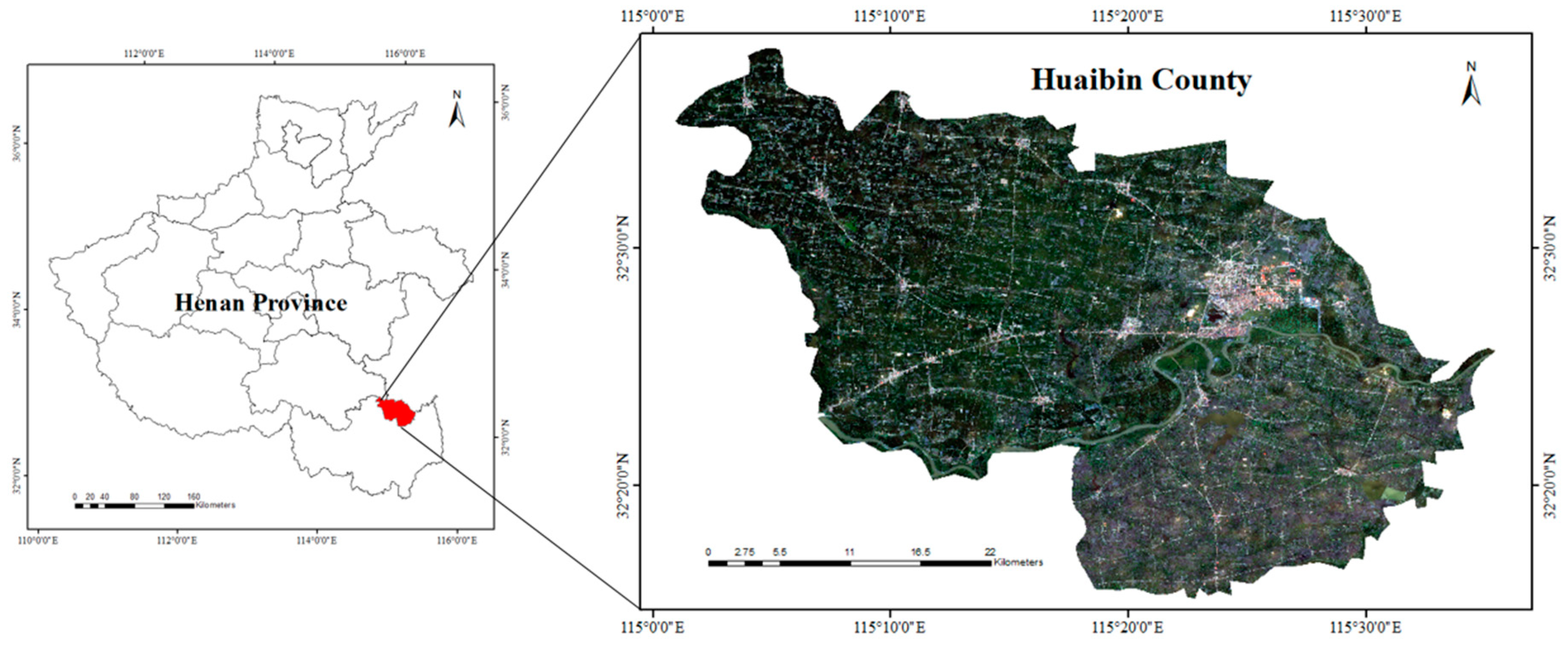
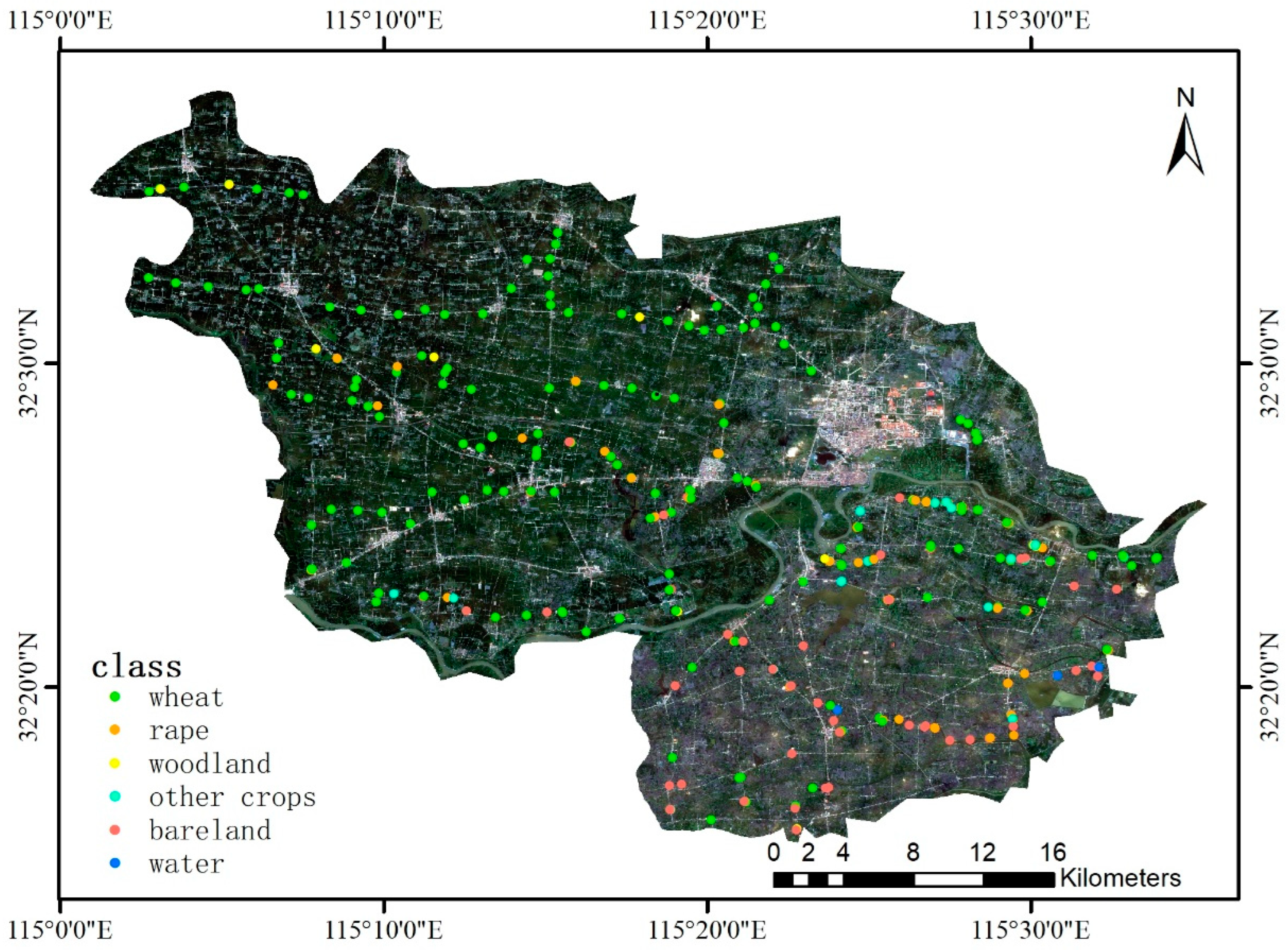
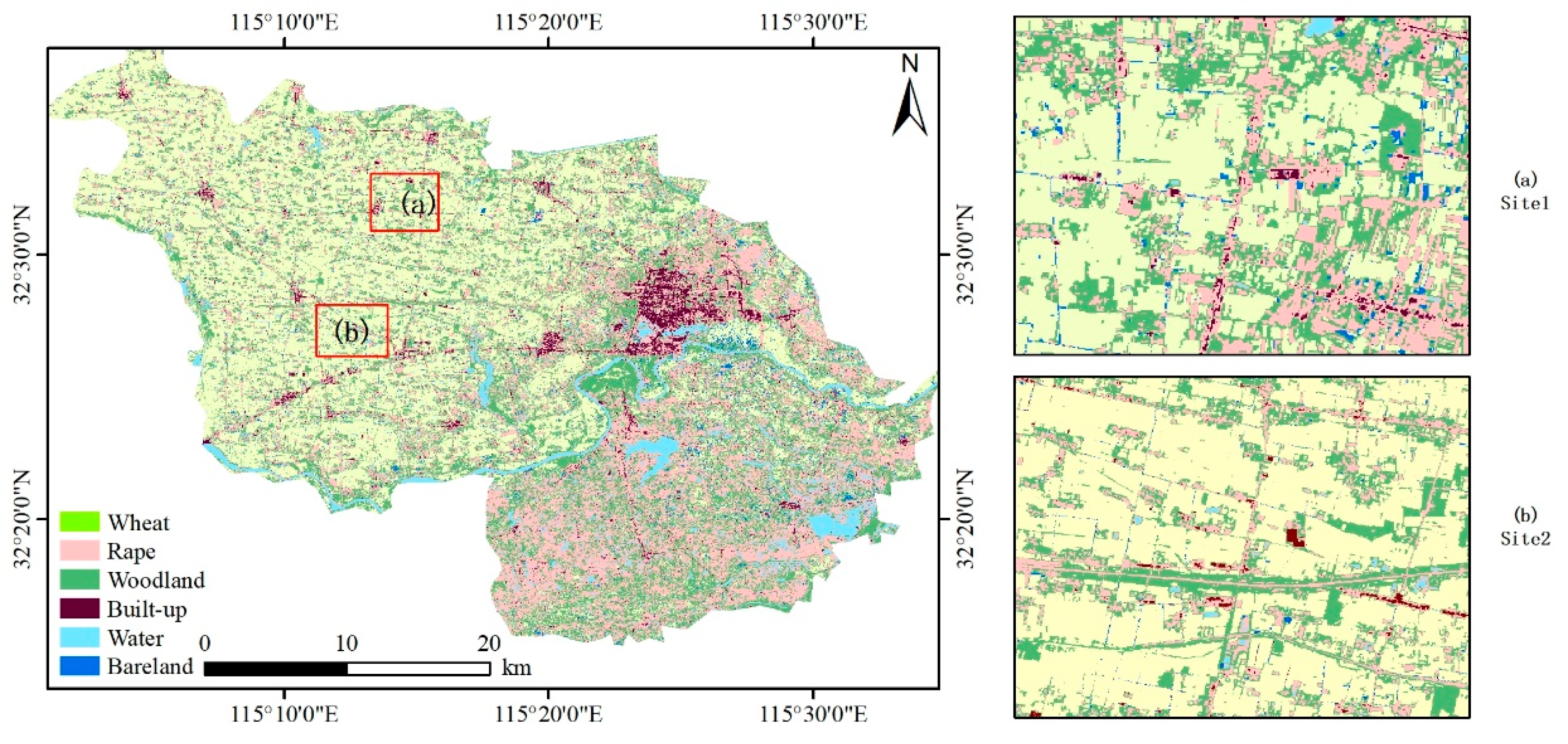
2.1. Study Area

In this study, we selected the typical wheat and oil crops production areas, namely Huaibin in Henan Province (Figure 1). Huaibin is northeastern in Xinyang City between 115°11′–115°35′ and 32°15′–32°38′. The total area of Huaibin County is 1209 square kilometer (Km2). Huaibin belongs to the transition zone of north subtropical and warm climate, with obvious monsoon climate and the same season of rain and heat. The mean annual air temperature was 15.6 °C during 2000–2021 from Huaibin. Located on the upper reaches of Huai River, Huaibin County is in the transition stage from the second ladder to the third ladder in China. The terrain slopes from west to east and gradually decreases from north to south, which can be divided into three types: hilly land, plain land and depression land. The main crop planting system in Huaibin is two crops per year, wheat and rape in winter, maize and rice in summer. The wheat and rape are usually planted in October and harvested in May. The different cropping cycles among these major crops provide the foundation to identify and map the crop fields in this study.

2.2. Datasets

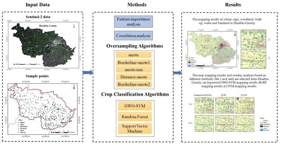
2.2.1. Sentinel-2 Data

Sentinel-2 satellite is a high-resolution multispectral imaging satellite designed for global terrestrial observations including terrestrial vegetation, soil, and water resources, inland waterways and coastal areas. Sentinel-2 image have high spectral and temporal resolutions and can be used to monitor crop area and growth using long time series images. Sentinel-2 comprises a constellation of two polar-orbiting satellites and provides imagery across 13 spectral bands, with a 10-day revisit period and a maximum spatial resolution of 10 m. Both satellites equipped with a multispectral instrument (MSI) that covers 13 spectral bands from visible light to short-wave infrared, with 10m, 20m and 60m resolution, respectively. In this study, we selected 9 Sentinel-2 remote sensing images from November 2020 to May 2021 during the main crop growing season. The Sentinel-2 Data (L2A-level image) were downloaded from the Google Earth Engine big data cloud platform. The band parameters of Sentinel-2 data are shown in Table 1.

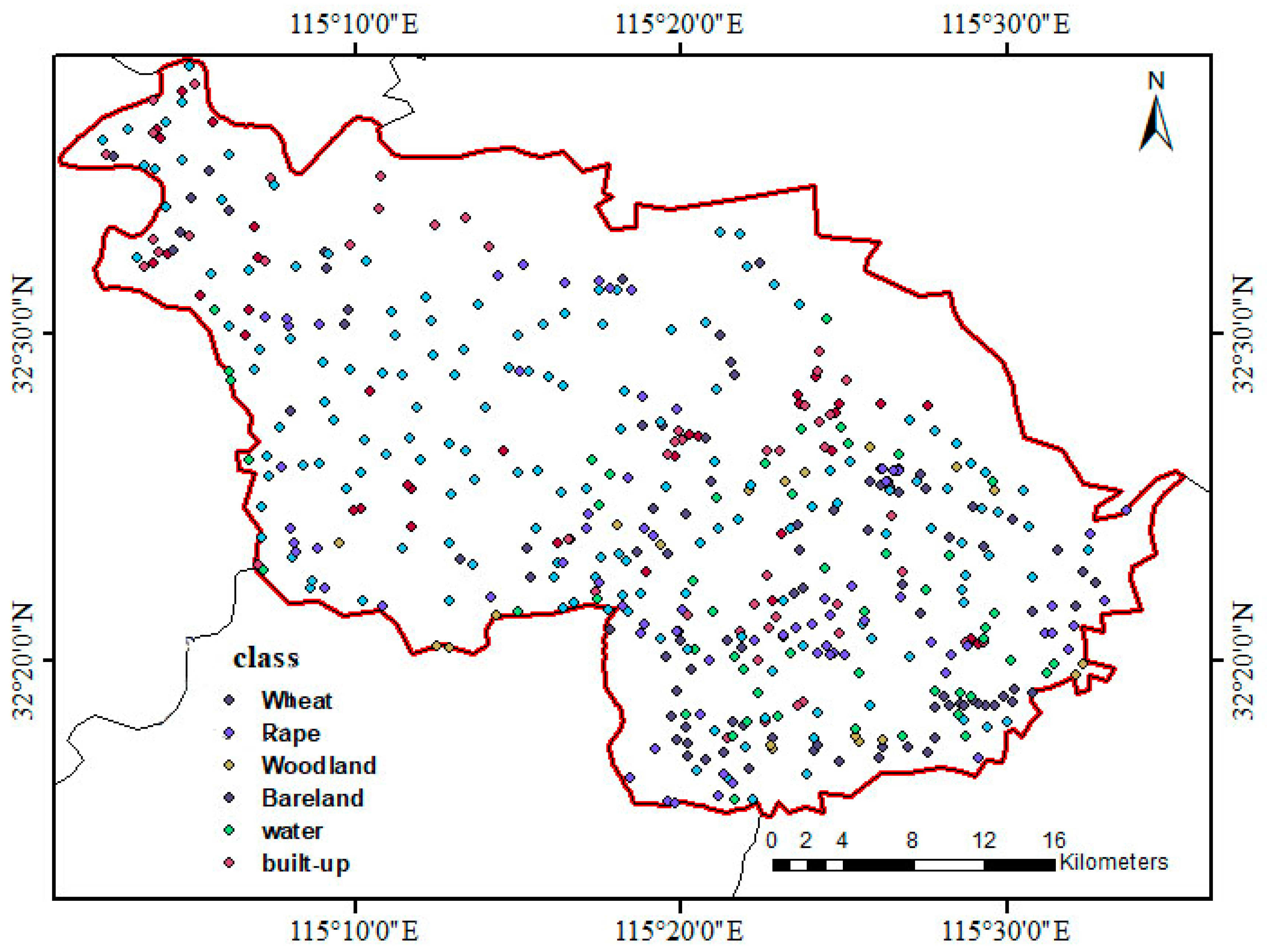
2.2.2. Field Sample Data

To obtain high-quality samples and ensure classification accuracy, a handheld GPS system was used to obtain ground data during crop maturity and harvest stage. From 25 May 2021 to 30 May 2021, we carried out field research in Huaibin. For example, winter wheat is in the maturity and harvest period, and the yield results are relatively stable, which facilitates the ground data collection. The field survey samples were collected by using handled GPS with a positioning accuracy of ±5 m. The collected data included crop types, growth situations, geographic coordinates and phenological periods. In 2021, 337 ground samples were taken: 174 samples of wheat, 68 samples of rape, 14 samples of woodland, 24 samples of other crops, 54 samples of bare land, 3 samples of water. The specific distribution of the samples is shown in Table 2 and Figure 2.

2.2.3. Visual Interpretation Data
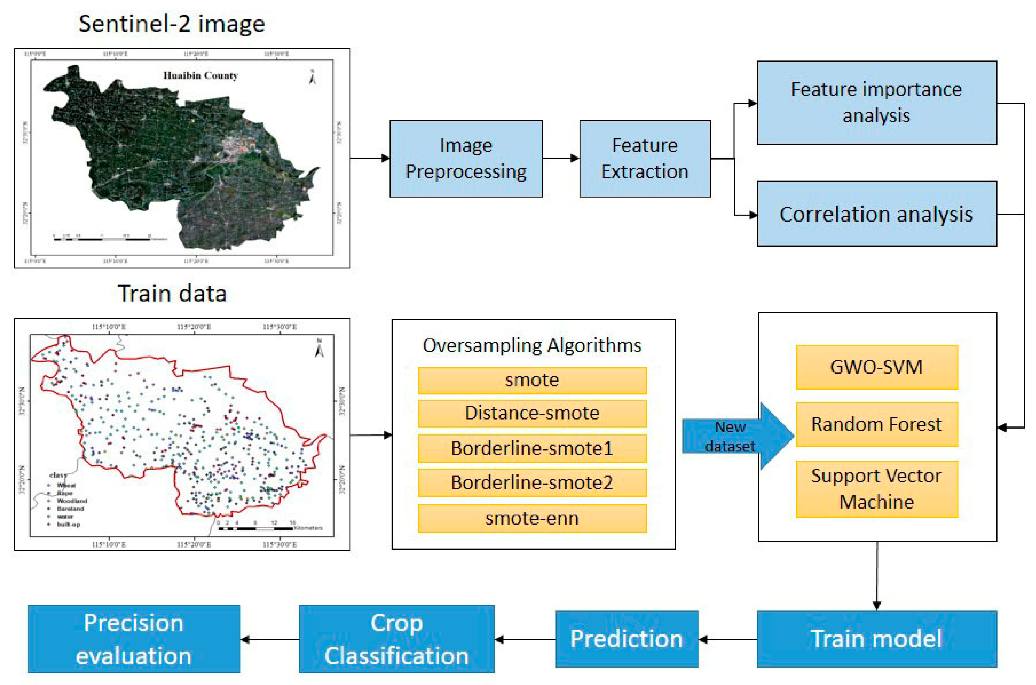
In order to obtain more sample points, we collected a large number of reference data from the high-resolution Google Earth image, including training sample points and test sample points (Figure 3) of wheat and rape, etc. Due to the differences in spectral and texture features of different crops in high spatial resolution images, sample points of crops were selected based on Google Earth images. When selecting samples, it is necessary to make full use of multi-temporal data and remote sensing image data combined with different bands, and use NDVI, EVI and other time series curves to judge different crop types. In order to improve the classification accuracy of samples, pure pixels should be selected. Table 3 is the number of visual interpretation sample points.

3. Methods

In order to effectively improve the classification accuracy of complex crops, the temporal remote sensing data of the whole growth period from November 2020 to May 2021 were selected in this study. In addition to the 10 spectral bands of Sentinel data, NDVI, EVI, SAVI, NDWI and NDBI were selected according to the characteristics of crop phenology, vegetation coverage, soil reflectance, moisture content and biomass in the study area. Then, Pearson and XGBoost methods are used to complete the correlation analysis and importance evaluation of all features, so as to optimize features and reduce feature redundancy. Previous studies have shown that sample imbalance will make the classification model more biased, which will not only lead to low accuracy of categories with fewer samples, but also affect the overall classification accuracy. Therefore, this study introduced oversampling methods, including smote, borderline-smote, smote-enn, distance-smote to solve the problem of sample imbalance in the classification process. Finally, combined with traditional classification methods such as GWO-SVM, SVM and random forest, the accuracy of classification results is compared based on user accuracy, producer accuracy, F1-score and overall accuracy. Figure 4 is the overall flow chart of this study.

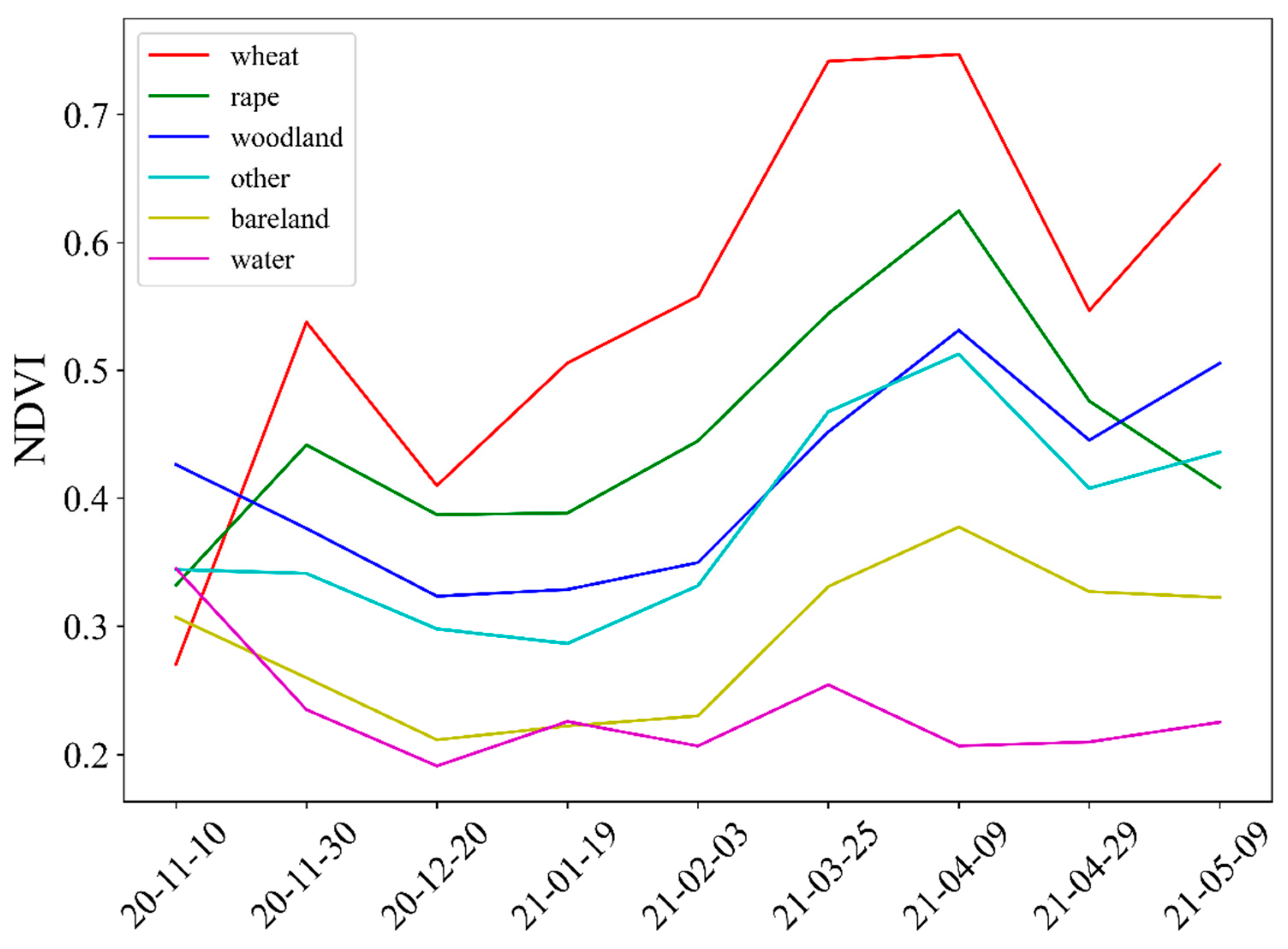
3.1. Time Series Vegetation Indexes

Vegetation index is sensitive to vegetation greenness and water status, which can obtain the physical differences of land use types. More emphasis on vegetation signals while reducing soil background and solar irradiance contributions. NDVI and Enhanced Vegetation Index (EVI) have high correlation with canopy leaf area index and chlorophyll, which can indicate the comprehensive changes of vegetation greenness and biomass. Normalized Difference Water Index (NDWI) reflects crop canopy water content and vegetation canopy water content. When vegetation is under water stress, NDWI can be accurately detected. Soil regulated vegetation index (SAVI) attempts to minimize the influence of soil brightness through soil brightness correction coefficient. The five vegetation indexes in Table 4 were initially selected for analysis.
Many studies have shown that the change of crop phenological characteristics in agricultural ecosystems is the most obvious. Using the difference of crop phenological characteristics can effectively improve the classification accuracy of complex crops and is also the basis for accurate monitoring of crops [43]. Crop phenological period reflects the growth and development of crops. Since the phenological periods of wheat, rape and other crops in the study area are relatively similar in a specific period of time, it is difficult to effectively distinguish the spectral characteristics, so it is difficult to effectively extract the crop planting area by using single-phase images. Therefore, based on the analysis of crop NDVI time series curve (Figure 5), this study completed the classification of wheat, rape, and other crops.

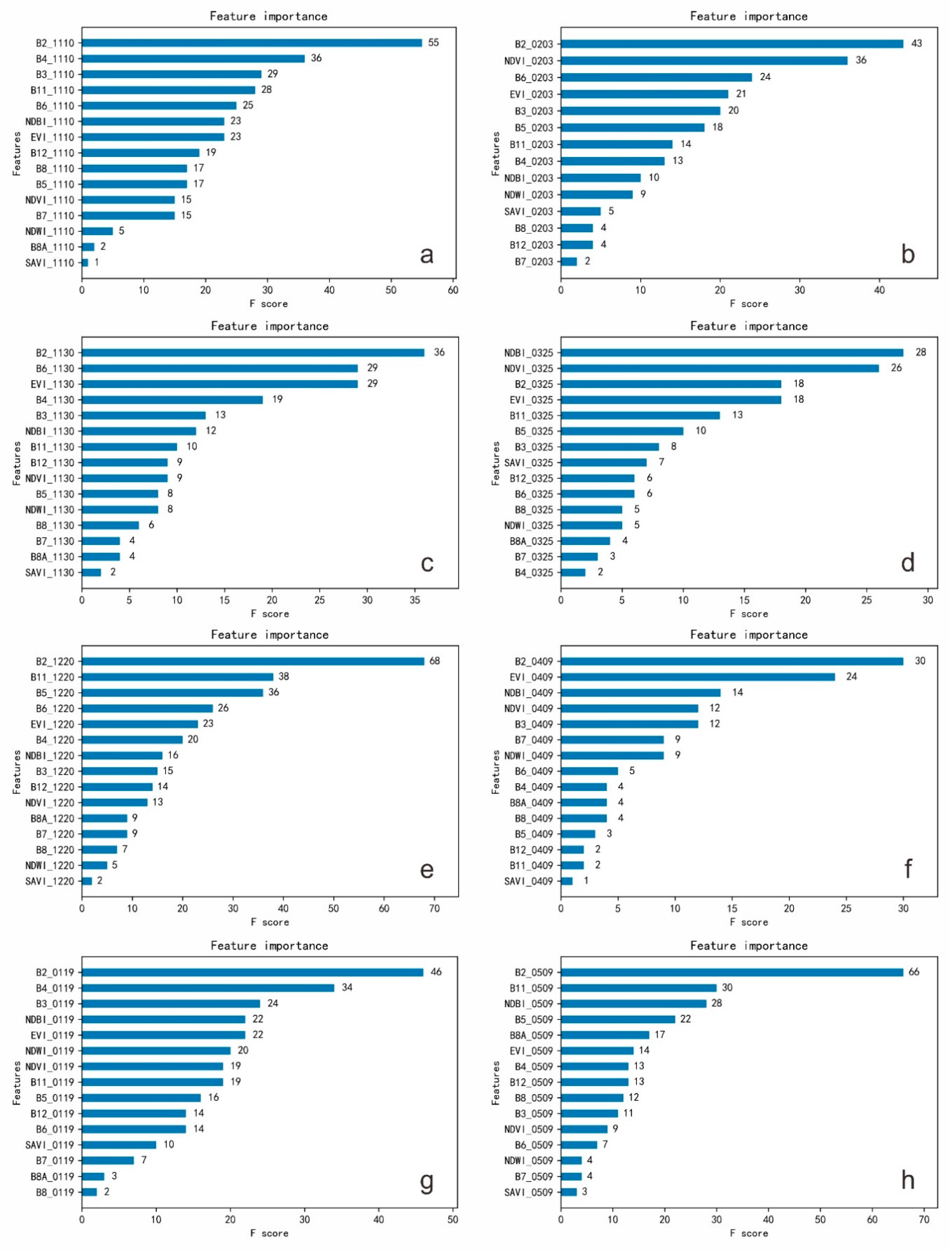
3.2. Feature Variable Optimization

Feature selection is an important method of feature dimension reduction in remote sensing image classification, and XGBoost has good effect in feature importance evaluation and correlation analysis. Based on python environment, this study uses XGBoost algorithm to achieve feature optimization. The XGBoost algorithm is an improved method based on GBDT model and a machine learning model based on Boosting idea. Compared with the traditional GBDT algorithm, it no longer uses the first-order derivative information, but is based on the second-order Taylor expansion, which can improve the efficiency of sorting the importance of input features and the optimal solution. Therefore, this study uses XGBoost model to evaluate the feature importance. In addition, based on the evaluation results of feature importance, Pearson correlation analysis is again used to reduce feature redundancy, and the Pearson coefficient standard is set to 0.9.

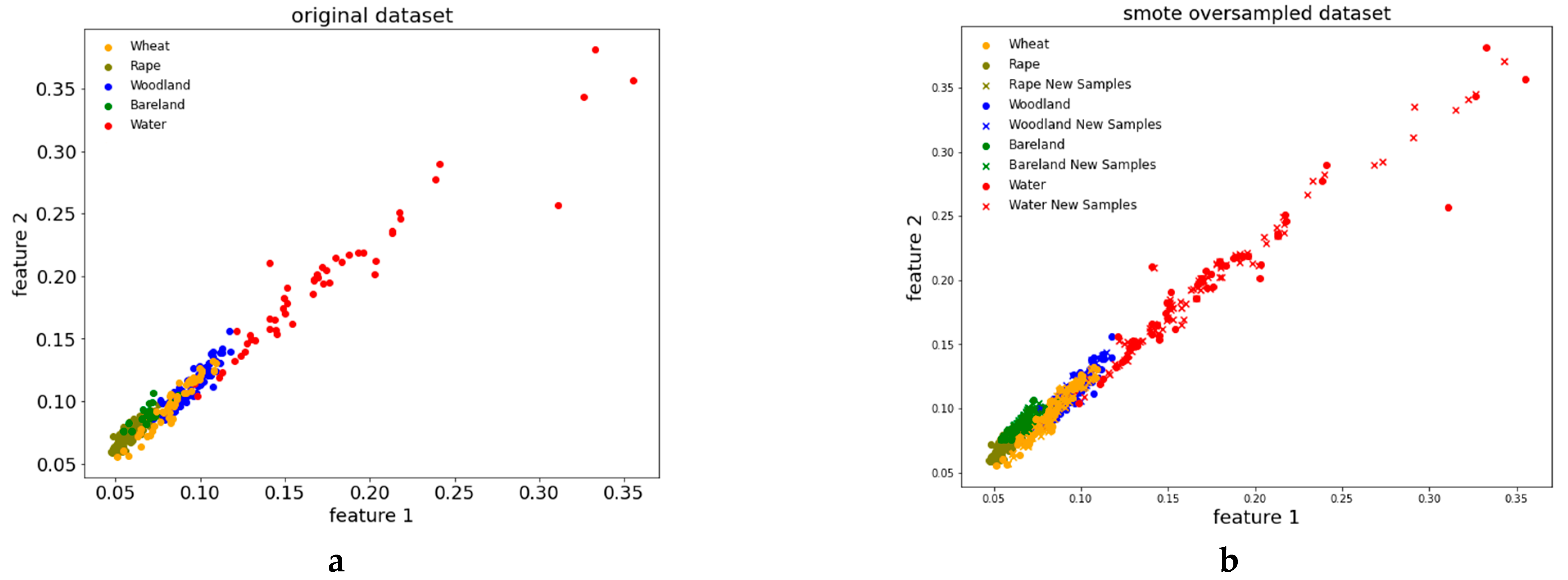
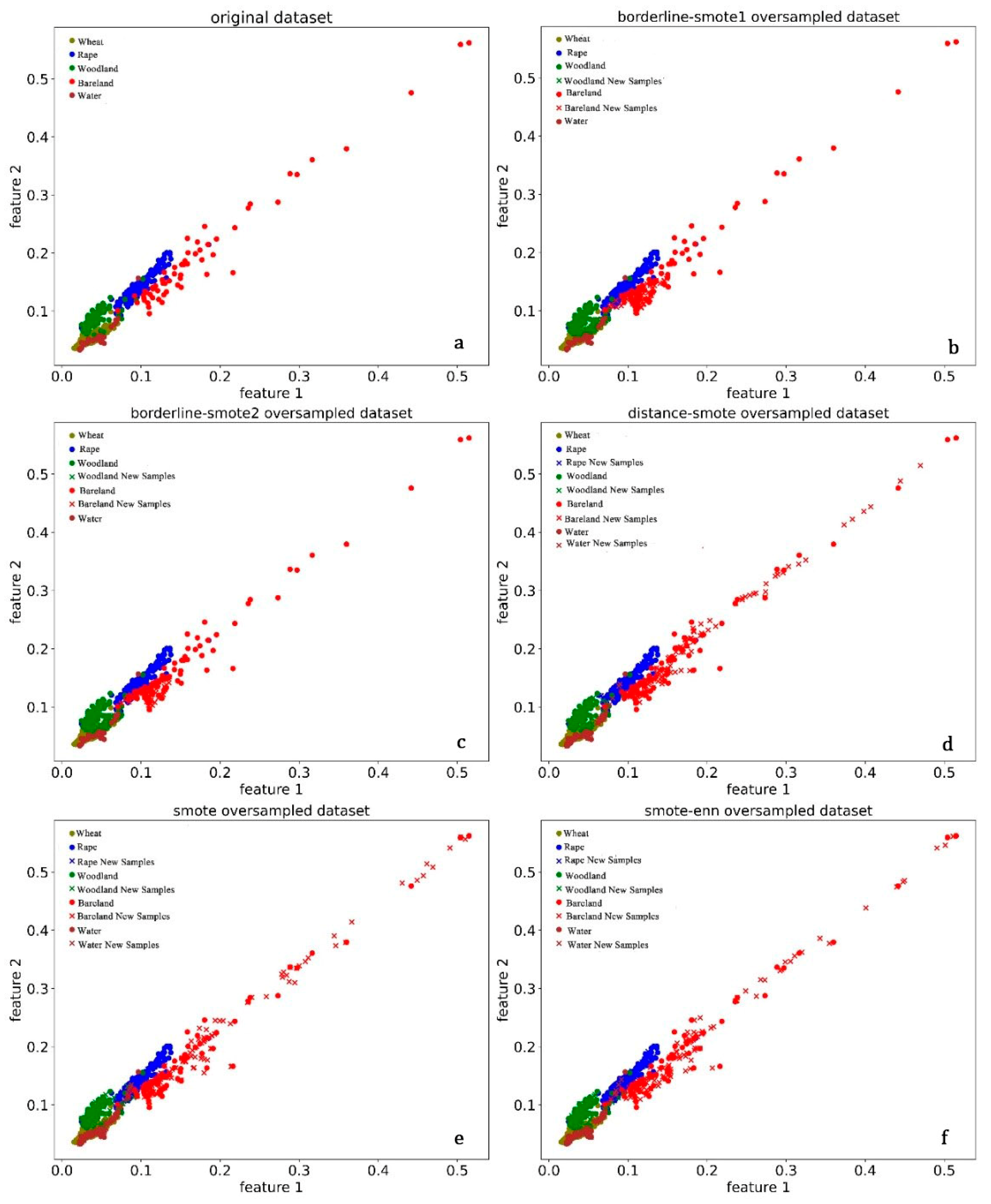
3.3. Oversampling Algorithm

Crop planting categories and spatial distribution usually cause the imbalance of samples in the classification process, which leads to the overrepresentation of large sample categories in the loss function in the traditional classification method. In order to solve the problem of sample imbalance, the existing research methods mainly include over-sampling of a few types of data or under-sampling of most types. Smote algorithm is an improved scheme based on random oversampling algorithm, which generates new samples by the difference between adjacent minority samples. The smote [44], Borderline-Smote [45] only conducted over-sampling for a few samples of boundary to improve the class distribution of samples, thereby improving the classification accuracy of a few samples. Distance-smote [46] assumed that the samples located at the edge of the class were more conducive to the formation of the classification boundary. The seed samples were obtained by directly comparing the distance and aggregation degree between the samples and the class center, and the new samples were synthesized on the connection between the seed samples and the class center. In this study, oversampling technique is used to solve the problem of sample imbalance in classification. The results before and after sampling are shown in Figure 6.

3.4. Selection of Classification Algorithms

In order to examine the performance of the improved GWO-SVM proposed in this study, it was compared with two supervised classification methods called random forest (RF) and support vector machine (SVM). Gray Wolf Optimizer is a new meta-inspired method that simulates the leadership level and hunting mechanism of l grey wolf in nature, and also realizes the three steps of hunting, searching for prey, enclosing prey, and attacking prey. Some studies show that compared with particle swarm optimization (PSO), gravitational search algorithm (GSA) and other algorithms, GWO algorithm [47] can provide very competitive results, which is suitable for challenging problems with unknown search space. In addition, GWO-SVM [48] can obtain the optimal parameters by iterative optimization to improve classification accuracy. Based on the above research results, this study uses the improved GWO-SVM method to realize the classification and extraction of complex crops, and compares it with traditional classification methods such as SVM, RF. Support vector machines uses kernel function to map linearly inseparable samples into high-dimensional linearly separable feature space, transforms the high-dimensional space problem into a quadratic programming problem, and obtains the global optimal solution through convex optimization, which is widely used in remote sensing image classification. Random forest is an ensemble learning method based on decision tree, which combines Bagging ensemble learning theory and random subspace method.

3.5. Accuracy Evaluation

To compare the accuracy of different classification methods, we randomly select training samples, and make the selected samples evenly distributed in the study area. Confusion matrix is a common accuracy evaluation index, so we select one of the evaluation indexes of confusion matrix. We also selected overall accuracy (OA), producer accuracy (PA), user accuracy (UA) and F1 score as evaluation indicators for crop mapping. The calculation method of each indicator is as follows.
O A = i = 1 n X i i X
P A = X i i X i *
U A = X i i X * i
F 1 i = 2 U A i P A i U A i + P A i
In the Equations (1)–(4), X is the total number of test samples, X i * and X * i are the total number of test samples of type i and the total number of samples of type i in the classification results, respectively. X i i is the number of the i-th row and the i-th column of the confusion matrix, indicating the number of correctly classified samples of the i-th category, and n is the number of classification categories.

4. Results

In this study, the Sentinel-2 time series image and its vegetation index were used to complete the feature selection. Based on the analysis of the processing performance of oversampling algorithms such as smote, smote-enn, borderline-smote1, borderline-smote2, distance-smote on imbalanced datasets, the effects of different methods on classification accuracy were evaluated. The classification results were compared with those of traditional classification methods, such as random forests and support vector machines, based on the indexes of computational efficiency, computational complexity and overall accuracy. Finally, the oversampling method with the optimal classification accuracy is selected. For the improved GWO-SVM, SVM and RF classification methods, the user accuracy, producer accuracy and F1 score classification index are used to evaluate the remote sensing classification effect of complex crops.

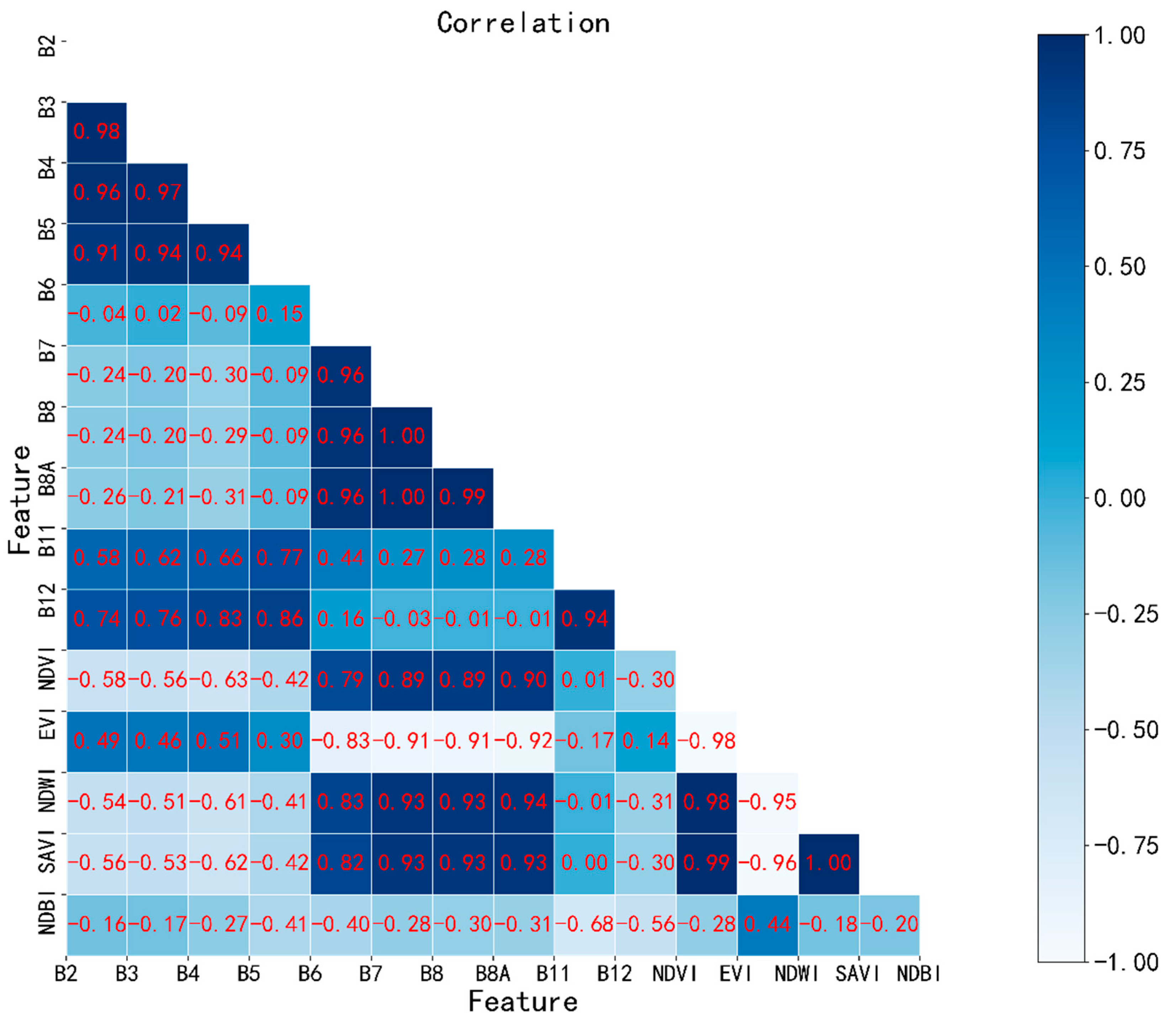
4.1. Feature Importance Analysis and Correlation Analysis

Feature importance evaluation is implemented by XGBoost package in python. By analyzing the feature importance of each month’s time series images. The feature importance result map from November 2020 to May 2021 is generated (Figure 7). Figure 7 shows that from November 2020 to May 2021, B2 is of high importance, which is caused by the high reflectivity of the bare ground and buildings. Then, the importance of NDVI gradually increased from October 2020 to March 2021, because crops such as wheat and rapeseed began to grow green after entering the seedling stage in November and entered the regreening period from February, were in the rapid growth stage. NDVI and EVI increased rapidly, which is an important indicator reflecting crop coverage and growth. In addition, the importance of B3, B4, and B6 is also higher, because the green, red and red edge bands are important spectral bands reflecting crop growth.
In this study, the correlation analysis was conducted on the selected 10 spectral band 5 vegetative indexes, and the correlation coefficients are shown in Figure 8. It can be seen that B2 has a higher correlation with B3 and B4, and the correlation coefficient is greater than 0.9. B6 has a higher correlation with B7, B8, and B8A, but its importance is weak. In the vegetation index, the correlation coefficients between NDVI and EVI and SAVI were 0.98 and 0.99, respectively, and the correlation coefficient between NDWI and SAVI reached 1.00.

4.2. Performance with Different Oversampling Algorithms

Figure 9 shows the overall distribution of the sample points. Among then, wheat as the main crop occupies the largest sample proportion, which is 51.32%, with other crops and buildings have fewer sample points. Existing studies has shown that when the ratio of the two types of samples in the dataset exceeds 1:2, the dataset can be considered to be imbalanced. Therefore, for the extremely imbalanced sample data in this study, smote, borderline-smote, smote-enn and distance-smote algorithms are, respectively used for processing. The results before and after processing are shown in Figure 10. It can be seen from Figure 10b that smote and smote-enn generate new samples based on a small number of class samples with boundaries differences. Borderline-smote1 and Borderline-smote2 generate new samples for the minority class samples at the border. Distance-smote compares the distance between the sample and the class center to obtain new samples.
Aiming at mitigating the impact of data sample imbalance on crop mapping, a combination of oversampling algorithms was proposed to achieve resampling. As shown in Table 5, comparisons were made between the distance-smote algorithm and other several single oversampling methods, namely the smote, smote-enn, Borderline-smote1 and Borderline-smote2 algorithms, on the basic of the raw data used in the training process. All the comparison experiments were based on the data randomly selected from the overall training crop samples. The training process was achieved with the GWO-SVM algorithm. As shown in Table 5, the accuracy of the raw data is the lowest, only 89.40%, while the accuracy is improved by using distance-smote methods, reaching 96.36%. Distance-smote on wheat and woodland had the highest producer accuracy, are 0.99 and 0.82. However, the producer accuracy on rape of Borderline-smote1 and Borderline-smote2 algorithms.

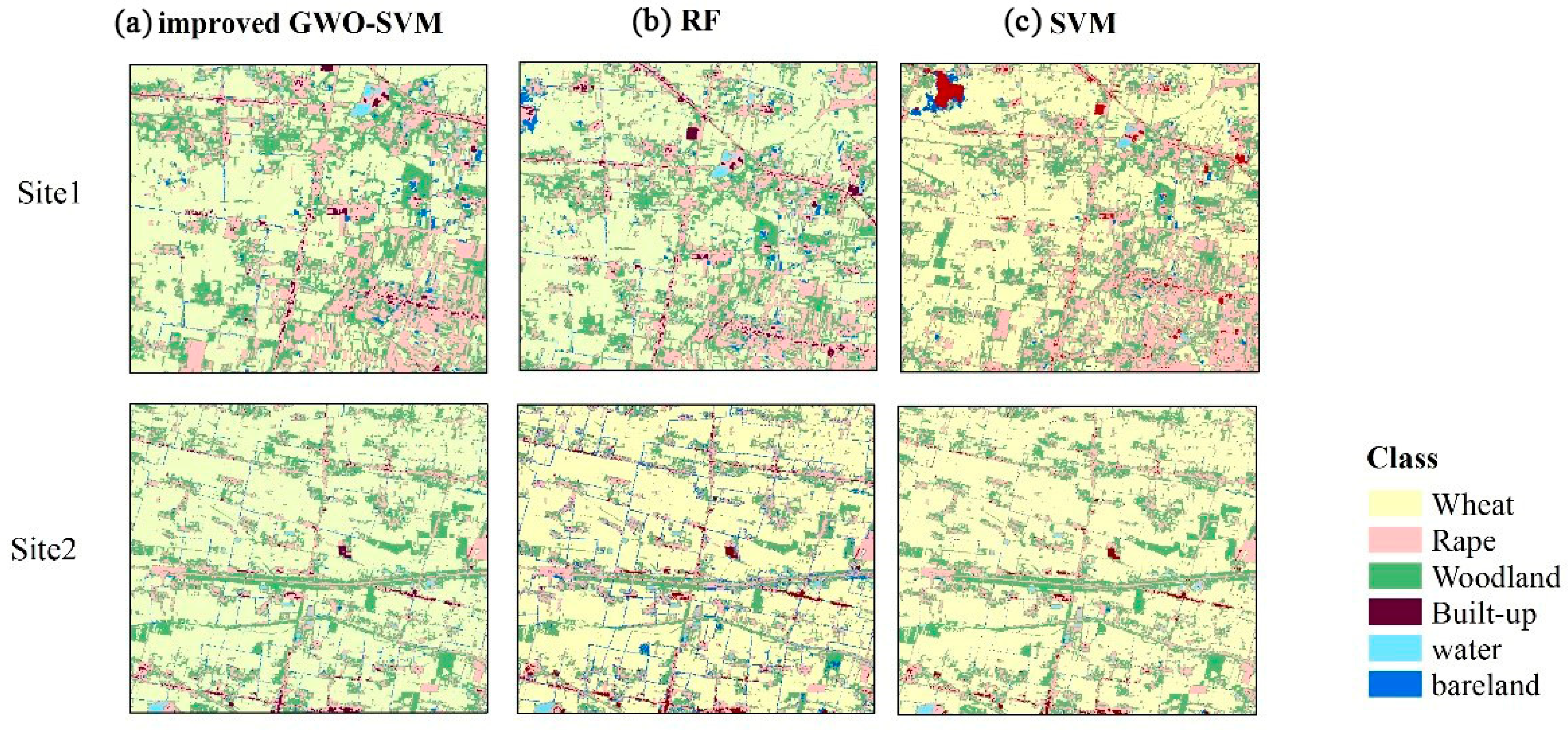
4.3. Comparison of Different Classification Methods

We have achieved the classification of the study area through different classification methods. Figure 11 shows the results of crop mapping for the entire county classified using the method proposed in this study. It can be seen that there are six categories, namely wheat, rape, woodland, buildings, water bodies and bare land, it can be seen from the figure that wheat is mainly distributed in the northern part of the Huai River, while rapeseed and woodland are mainly distributed in the southern part of the Huai River. This article compares SVM and Random Forest, which have performed well in crop mapping in recent years. Mainly compare the overall accuracy of different crops in the study area, F1-score, user accuracy and producer accuracy.
The output results of the Pearson correlation matrix can be seen from Fig. 8 that wheat is mainly distributed in the north of Huai River, and rape and woodland are mainly distributed in the south of Huai River. The study area covers an area of 1291 Km2. The error was small, which was also in line with the field survey results. Therefore, this study can provide technical reference for the accurate classification of crops at the county level. Table 6 is the classification results of three classification methods based on GWO-SVM, including overall accuracy, F1-score, user accuracy and producer accuracy. It can be seen from Table 5 that the overall accuracy of the improved GWO-SVM is 96.36%, and the user accuracy of rape and built-up is also significantly higher than the other two classification methods. In addition, in order to further verify the classification results of different methods, we randomly selected two regions in the study area for comparisons. It can be seen that the crop plots extracted based on the improved GWO-SVM method in Figure 12a are more regular and less salt and pepper phenomenon. However, the classification result of RF model in Figure 12b are relatively fragmented, and the SVM method in Figure 12b also misclassified the rape and the building. Compared with the improved GWO-SVM, RF and SVM have a poorer extraction effect on narrow rural roads, and there are misclassifications of wheat and rape, and support vector machine has more misclassification of woodland. Further details can be found in the discussion.

5. Discussion

5.1. The Significance of Feature Selection

Due to the diversified crops and high filed fragmentation, it is necessary to select remote sensing image data for crop mapping. As shown in Figure 5, the time-series NDVI of different categories is different in specific growth periods, especially winter wheat shows an obvious upward trend in November and a downward trend in December. This is because after wheat enters the seedling and tillering stages, the vegetation coverage increases, and then stops growing at the overwintering stage. After February of the next year, the winter wheat was in the rising stage and jointing stage, the rapid growth of NDVI and EVI vegetation index showed an upward trend. After May, the winter wheat gradually entered the mature stage, and the chlorophyll content decrease, which also led to vegetation index showed a gentle downward trend. Rapeseed declined after a slow rise from November to December due to lower surface coverage at seedling stage and reduced chlorophyll content after wintering. From March to May, the vegetation index increased first and then decreased. The reason is similar to that of winter wheat, which is due to the influence of vegetation physiological characteristics such as fractional cover and canopy characteristics, leaf green content and so on. Therefore, it is necessary to classify crops with similar spectral characteristics by using multi-temporal image data and feature selection. Audrey Mercier [49] used multi-temporal Sentinel-1 and Sentinel-2 time series images to distinguish wheat from rape and found that leaf area index (LAI) and NDVI were the most important.
The above research is consistent with the conclusion that the use satellite images can improve the classification accuracy of complex crops. In terms of feature selection, this paper realizes the importance evaluation and correlation analysis based on XGBoost package and Pearson coefficient. The results showed that NDVI, EVI, SAVI and B2, B8A had high feature importance in crop classification model, and the correlation between NDVI and SAVI was 0.99. Wang et al. [50] found that B2 and NDVI have high characteristic importance based on RF classification method in winter crop mapping in complex agricultural areas, which is consistent with the conclusion of this study. In summary, by analyzing and optimizing the spectral and vegetation index characteristics of different crops, this study not only reduces the feature redundancy and improves the classification accuracy, but also provides a more efficient method for the classification of complex crops at county scale.

5.2. Role of Oversampling Algorithms

In this study, five oversampling algorithms, smote, smote-enn, distance-smote, borderline-smote1, borderline-smote2, to solve the problem of sample data imbalance. The accuracy was improved by 1.2%, 2.5%, 3.2%, 4.5% and 3.1%, respectively, compared with imbalanced data Lin et al. [36] used the smote-enn oversampling technique to solve the problem of small proportion of strong scintillation in datasets, and the accuracy was improved by 4–5% compared with decision trees and random forests. Zhang et al. [9] used borderline-smote to study the problem of susceptibility of debris flow, and the results were about 15% higher than the imbalanced. In this study, five oversampling techniques are applied to solve the sample imbalance problems, and the distance-smote method shows remarkable performance in solving this problem. However, smote aims to increase the number of minority classes and improves the classification accuracy of small sample classes such as rape, but the accuracy of major classes has not improved significantly. Therefore, in the next step, this study should combine the undersampling method to improve and solve the classification accuracy problem caused by sample imbalance in general.

5.3. Compare Different Classification Algorithms

In order to compare different classification algorithms, imbalanced crop sample test datasets were established. The results significantly illustrate the excellent performance of the improved GWO-SVM in crop classification. It can be shown in Table 5 that the accuracy of the improved GWO-SVM was higher than SVM and RF. The overall testing accuracy of the improved GWO-SVM is 96.36%, higher than SVM 1.1% and higher than RF 0.8%. The F1 score of the improved GWO-SVM is 0.96, higher than SVM 2%. Compared to wheat, the rape and bareland are minor class. The PA of Rape are minor class. In the rape class, the producer accuracy of the improved GWO-SVM algorithm was 5% and 8% higher than that of SVM and RF, respectively. In the bareland class, the user accuracy of the improved GWO-SVM algorithm was 1% and 1% higher than that of SVM and RF, respectively. These results indicate that it is valuable to enhance the detection accuracy for strong scintillation events with different degrees of imbalance in the testing data with the method of resampling the imbalanced training data by distance-smote before training the GWO-SVM model.
In this paper, SVM with GWO optimization algorithm not only improves the classification efficiency and accuracy of complex crops, but also has strong global search ability. In addition, parameter A also controls the local search part range of the algorithm, making the global search ability and local search ability relatively balanced, which is an improvement to the firefly algorithm. However, GWO-SVM still has some limitations, that is, in the face of complex optimization problems, there is a slow convergence in the later stage.

6. Conclusions

Timely and accurate crop mapping is the basis for government decision-making and evaluation of agricultural production. Crop classification results provide basic data support for planting structure optimization and production decisions.
In this study, the importance evaluation and correlation analysis were completed based on the characteristics of time series Sentinel-2 image spectral and vegetation index. The smote, Borderline-smote1, Borderline-smote2, smote-enn and distance-smote oversampling methods were used to solve the imbalance problem of minority class samples in the procedure. We found the distance-smote performed the best. Finally, GWO-SVM, RF, SVM and other methods were used to complete the comparative analysis of complex crop mapping results. It is found that NDVI and EVI are of high importance, and B2, B4, B6, and B11 are more important. In this study, the classification accuracy was improved by feature selection. Therefore, it is necessary to conduct feature importance evaluation and correlation analysis for feature selection in the classification procedure. In the imbalanced processing of sample points, it is found that the user accuracy and producer accuracy of the classification results are higher than those of the imbalanced processing by using smote, borderline-smote1, borderline-smote2, distance-smote, and smote-enn methods. In addition, studies have shown that distance-smote can improve the classification accuracy and classification efficiency of complex crops to the greatest extent. Therefore, this work will provide reference for researchers who use imbalanced samples to classify crops, and the crops will provide necessary information for the management of local wheat and oil crops.

Author Contributions

Conceptualization, M.G. and H.Z.; methodology, H.Z.; software, H.Z.; validation, M.G., and C.R.; formal analysis, H.Z.; writing—original draft preparation H.Z. and M.G.; writing—review and editing, M.G. and C.R.; supervision, M.G, and C.R.; funding acquisition, M.G. All authors have read and agreed to the published version of the manuscript.

Funding

This research was supported by the National Natural Science Foundation of China (41871282).

Institutional Review Board Statement

Not applicable.

Informed Consent Statement

Not applicable.

Conflicts of Interest

The authors declare no conflict of interest.

References

  1. Adrian, J.; Sagan, V.; Maimaitijiang, M. Sentinel SAR-optical fusion for crop type mapping using deep learning and Google Earth Engine. Isprs J. Photogramm. 2021, 175, 215–235. [Google Scholar] [CrossRef]
  2. Brinkhoff, J.; Vardanega, J.; Robson, A.J. Land Cover Classification of Nine Perennial Crops Using Sentinel-1 and-2 Data. Remote Sens. 2020, 12, 96. [Google Scholar] [CrossRef] [Green Version]
  3. Phiri, D.; Simwanda, M.; Salekin, S.; Nyirenda, V.R.; Murayama, Y.; Ranagalage, M. Sentinel-2 Data for Land Cover/Use Mapping: A Review. Remote Sens. 2020, 12, 2291. [Google Scholar] [CrossRef]
  4. Zhang, C.Y.; Marzougui, A.; Sankaran, S. High-resolution satellite imagery applications in crop phenotyping: An overview. Comput. Electron. Agric. 2020, 175, 105584. [Google Scholar] [CrossRef]
  5. Qadir, A.; Mondal, P. Synergistic Use of Radar and Optical Satellite Data for Improved Monsoon Cropland Mapping in India. Remote Sens. 2020, 12, 522. [Google Scholar] [CrossRef] [Green Version]
  6. Ramadhani, F.; Pullanagari, R.; Kereszturi, G.; Procter, J. Automatic Mapping of Rice Growth Stages Using the Integration of SENTINEL-2, MOD13Q1, and SENTINEL-1. Remote Sens. 2020, 12, 3613. [Google Scholar] [CrossRef]
  7. Dheeravath, V.; Thenkabail, P.S.; Chandrakantha, G.; Noojipady, P.; Reddy, G.P.O.; Biradar, C.M.; Gumma, M.K.; Velpuri, M. Irrigated areas of India derived using MODIS 500 m time series for the years 2001–2003. Isprs J. Photogramm. 2010, 65, 42–59. [Google Scholar] [CrossRef]
  8. Potgieter, A.B.; Apan, A.; Hammer, G.; Dunn, P. Early-season crop area estimates for winter crops in NE Australia using MODIS satellite imagery. Isprs J. Photogramm. 2010, 65, 380–387. [Google Scholar] [CrossRef]
  9. Zhang, B.; Liu, X.; Liu, M.; Meng, Y. Detection of Rice Phenological Variations under Heavy Metal Stress by Means of Blended Landsat and MODIS Image Time Series. Remote Sens. 2019, 11, 13. [Google Scholar] [CrossRef] [Green Version]
  10. Yang, H.J.; Pan, B.; Wu, W.F.; Tai, J.H. Field-based rice classification in Wuhua county through integration of multi-temporal Sentinel-1A and Landsat-8 OLI data. Int. J. Appl. Earth Obs. 2018, 69, 226–236. [Google Scholar] [CrossRef]
  11. Bolivar-Santamaria, S.; Reu, B. Detection and characterization of agroforestry systems in the Colombian Andes using Sentinel-2 imagery. Agrofor. Syst. 2021, 95, 499–514. [Google Scholar] [CrossRef]
  12. Ren, T.W.; Liu, Z.; Zhang, L.; Liu, D.Y.; Xi, X.J.; Kang, Y.H.; Zhao, Y.Y.; Zhang, C.; Li, S.M.; Zhang, X.D. Early Identification of Seed Maize and Common Maize Production Fields Using Sentinel-2 Images. Remote Sens. 2020, 12, 2140. [Google Scholar] [CrossRef]
  13. Preidl, S.; Lange, M.; Doktor, D. Introducing APiC for regionalised land cover mapping on the national scale using Sentinel-2A imagery. Remote Sens. Environ. 2020, 240, 111673. [Google Scholar] [CrossRef]
  14. Granzig, T.; Fassnacht, F.E.; Kleinschmit, B.; Forster, M. Mapping the fractional coverage of the invasive shrub Ulex europaeus with multi-temporal Sentinel-2 imagery utilizing UAV orthoimages and a new spatial optimization approach. Int. J. Appl. Earth Obs. 2021, 96, 102281. [Google Scholar] [CrossRef]
  15. Wang, X.Y.; Guo, Y.G.; He, J.; Du, L.T. Fusion of HJ1B and ALOS PALSAR data for land cover classification using machine learning methods. Int. J. Appl. Earth Obs. 2016, 52, 192–203. [Google Scholar] [CrossRef]
  16. Tetila, E.C.; Machado, B.B.; Belete, N.A.D.; Guimaraes, D.A.; Pistori, H. Identification of Soybean Foliar Diseases Using Unmanned Aerial Vehicle Images. IEEE Geosci. Remote Sens. Lett. 2017, 14, 2190–2194. [Google Scholar] [CrossRef]
  17. Sinha, P.; Robson, A.; Schneider, D.; Kilic, T.; Mugera, H.K.; Ilukor, J.; Tindamanyire, J.M. The potential of in-situ hyperspectral remote sensing for differentiating 12 banana genotypes grown in Uganda. Isprs J. Photogramm. 2020, 167, 85–103. [Google Scholar] [CrossRef]
  18. Sonobe, R.; Yamaya, Y.; Tani, H.; Wang, X.F.; Kobayashi, N.; Mochizuki, K. Mapping crop cover using multi-temporal Landsat 8 OLI imagery. Int. J. Remote Sens. 2017, 38, 4348–4361. [Google Scholar] [CrossRef] [Green Version]
  19. Zhang, H.Y.; Du, H.Y.; Zhang, C.K.; Zhang, L.P. An automated early-season method to map winter wheat using time-series Sentinel-2 data: A case study of Shandong, China. Comput. Electron. Agric. 2021, 182, 105962. [Google Scholar] [CrossRef]
  20. Asgarian, A.; Soffianian, A.; Pourmanafi, S. Crop type mapping in a highly fragmented and heterogeneous agricultural landscape: A case of central Iran using multi-temporal Landsat 8 imagery. Comput. Electron. Agric. 2016, 127, 531–540. [Google Scholar] [CrossRef]
  21. Gallo, I.; La Grassa, R.; Landro, N.; Boschetti, M. Sentinel 2 Time Series Analysis with 3D Feature Pyramid Network and Time Domain Class Activation Intervals for Crop Mapping. Isprs Int. J. Geo-Inf. 2021, 10, 483. [Google Scholar] [CrossRef]
  22. Skakun, S.; Franch, B.; Vermote, E.; Roger, J.C.; Becker-Reshef, I.; Justice, C.; Kussul, N. Early season large-area winter crop mapping using MODIS NDVI data, growing degree days information and a Gaussian mixture model. Remote Sens. Environ. 2017, 195, 244–258. [Google Scholar] [CrossRef]
  23. Pageot, Y.; Baup, F.; Inglada, J.; Baghdadi, N.; Demarez, V. Detection of Irrigated and Rainfed Crops in Temperate Areas Using Sentinel-1 and Sentinel-2 Time Series. Remote Sens. 2020, 12, 3044. [Google Scholar] [CrossRef]
  24. Wang, L.J.; Wang, J.Y.; Zhang, X.W.; Wang, L.G.; Qin, F. Deep segmentation and classification of complex crops using multi-feature satellite imagery. Comput. Electron. Agric. 2022, 200, 107249. [Google Scholar] [CrossRef]
  25. Wang, L.J.; Wang, J.Y.; Liu, Z.Z.; Zhu, J.; Qin, F. Evaluation of a deep-learning model for multispectral remote sensing of land use and crop classification. Crop J. 2022, 10, 1435–1451. [Google Scholar] [CrossRef]
  26. Sitokonstantinou, V.; Papoutsis, I.; Kontoes, C.; Lafarga Arnal, A.; Armesto Andres, A.P.; Garraza Zurbano, J.A. Scalable Parcel-Based Crop Identification Scheme Using Sentinel-2 Data Time-Series for the Monitoring of the Common Agricultural Policy. Remote Sens. 2018, 10, 911. [Google Scholar] [CrossRef] [Green Version]
  27. Pena, J.M.; Gutierrez, P.A.; Hervas-Martinez, C.; Six, J.; Plant, R.E.; Lopez-Granados, F. Object-Based Image Classification of Summer Crops with Machine Learning Methods. Remote Sens. 2014, 6, 5019–5041. [Google Scholar] [CrossRef] [Green Version]
  28. Arango, R.B.; Campos, A.M.; Combarro, E.F.; Canas, E.R.; Diaz, I. Mapping cultivable land from satellite imagery with clustering algorithms. Int. J. Appl. Earth Obs. 2016, 49, 99–106. [Google Scholar] [CrossRef]
  29. Pena-Arancibia, J.L.; McVicar, T.R.; Paydar, Z.; Li, L.T.; Guerschman, J.P.; Donohue, R.J.; Dutta, D.; Podger, G.M.; van Dijk, A.I.J.M.; Chiew, F.H.S. Dynamic identification of summer cropping irrigated areas in a large basin experiencing extreme climatic variability. Remote Sens. Environ. 2014, 154, 139–152. [Google Scholar] [CrossRef]
  30. de Castro, H.C.; de Carvalho, O.A.; de Carvalho, O.L.F.; de Bem, P.P.; de Moura, R.D.; de Albuquerque, A.O.; Silva, C.R.; Ferreira, P.H.G.; Guimaraes, R.F.; Gomes, R.A.T. Rice Crop Detection Using LSTM, Bi-LSTM, and Machine Learning Models from Sentinel-1 Time Series. Remote Sens. 2020, 12, 2655. [Google Scholar]
  31. Sheykhmousa, M.; Mahdianpari, M.; Ghanbari, H.; Mohammadimanesh, F.; Ghamisi, P.; Homayouni, S. Support Vector Machine Versus Random Forest for Remote Sensing Image Classification: A Meta-Analysis and Systematic Review. IEEE J. Stars 2020, 13, 6308–6325. [Google Scholar] [CrossRef]
  32. Li, R.Y.; Xu, M.Q.; Chen, Z.Y.; Gao, B.B.; Cai, J.; Shen, F.X.; He, X.L.; Zhuang, Y.; Chen, D.L. Phenology-based classification of crop species and rotation types using fused MODIS and Landsat data: The comparison of a random-forest-based model and a decision-rule-based model. Soil Tillage Res. 2021, 206, 104838. [Google Scholar] [CrossRef]
  33. Xu, J.F.; Zhu, Y.; Zhong, R.H.; Lin, Z.X.; Xu, J.L.; Jiang, H.; Huang, J.F.; Li, H.F.; Lin, T. DeepCropMapping: A multi-temporal deep learning approach with improved spatial generalizability for dynamic corn and soybean mapping. Remote Sens. Environ. 2020, 247, 111946. [Google Scholar] [CrossRef]
  34. Samui, P.; Gowda, P.H.; Oommen, T.; Howell, T.A.; Marek, T.H.; Porter, D.O. Statistical learning algorithms for identifying contrasting tillage practices with Landsat Thematic Mapper data. Int. J. Remote Sens. 2012, 33, 5732–5745. [Google Scholar] [CrossRef]
  35. Low, F.; Michel, U.; Dech, S.; Conrad, C. Impact of feature selection on the accuracy and spatial uncertainty of per-field crop classification using Support Vector Machines. Isprs J. Photogramm. 2013, 85, 102–119. [Google Scholar] [CrossRef]
  36. Lin, M.; Zhu, X.; Hua, T.; Tang, X.; Tu, G.; Chen, X. Detection of Ionospheric Scintillation Based on XGBoost Model Improved by SMOTE-ENN Technique. Remote Sens. 2021, 13, 2577. [Google Scholar] [CrossRef]
  37. Wang, N.; Cheng, W.M.; Zhao, M.; Liu, Q.Y.; Wang, J. Identification of the Debris Flow Process Types within Catchments of Beijing Mountainous Area. Water 2019, 11, 638. [Google Scholar] [CrossRef] [Green Version]
  38. Farrar, T.J.; Nicholson, S.E.; Lare, A.R. The influence of soil type on the relationships between NDVI, rainfall, and soil moisture in semiarid Botswana. II. NDVI response to soil moisture. Remote Sens. Environ. 1994, 50, 121–133. [Google Scholar] [CrossRef]
  39. Liu, H.Q.; Huete, A. A Feedback Based Modification of the Ndvi to Minimize Canopy Background and Atmospheric Noise. IEEE T Geosci. Remote 1995, 33, 457–465. [Google Scholar] [CrossRef]
  40. Huete, A.R. A soil-adjusted vegetation index (SAVI). Remote Sens. Environ. 1988, 25, 295–309. [Google Scholar] [CrossRef]
  41. McFeeters, S.K. The use of the normalized difference water index (NDWI) in the delineation of open water features. Int. J. Remote Sens. 1996, 17, 1425–1432. [Google Scholar] [CrossRef]
  42. Zha, Y.; Gao, J.; Ni, S. Use of normalized difference built-up index in automatically mapping urban areas from TM imagery. Int. J. Remote Sens. 2003, 24, 583–594. [Google Scholar] [CrossRef]
  43. Valcarce-Dineiro, R.; Arias-Perez, B.; Lopez-Sanchez, J.M.; Sanchez, N. Multi-Temporal Dual- and Quad-Polarimetric Synthetic Aperture Radar Data for Crop-Type Mapping. Remote Sens. 2019, 11, 1518. [Google Scholar] [CrossRef] [Green Version]
  44. .Chawla, N.V.; Bowyer, K.W.; Hall, L.O.; Kegelmeyer, W.P. SMOTE: Synthetic minority over-sampling technique. J. Artif. Intell. Res. 2002, 16, 321–357. [Google Scholar] [CrossRef]
  45. Han, H.; Wang, W.Y.; Mao, B.H. Borderline-SMOTE: A New Over-Sampling Method in Imbalanced Data Sets Learning. In Advances in Intelligent Computing, Pt 1, Proceedings; Huang, D.S., Zhang, X.P., Huang, G.B., Eds.; Lecture Notes in Computer Science; Springer: Berlin, Germany, 2005; Volume 3644, pp. 878–887. [Google Scholar]
  46. Bunkhumpornpat, C.; Sinapiromsaran, K.; Lursinsap, C. DBSMOTE: Density-Based Synthetic Minority Over-sampling TEchnique. Appl. Intell. 2012, 36, 664–684. [Google Scholar] [CrossRef]
  47. Mirjalili, S.; Mirjalili, S.M.; Lewis, A. Grey Wolf Optimizer. Adv. Eng. Softw. 2014, 69, 46–61. [Google Scholar] [CrossRef] [Green Version]
  48. Sweidan, A.H.; El-Bendary, N.; Hassanien, A.E.; Hegazy, O.M.; Mohamed, A.E.-K. Water Quality Classification Approach based on Bio-Inspired Gray Wolf Optimization. In Proceedings of the 2015 Seventh International Conference of Soft Computing and Pattern Recognition, Fukuoka, Japan, 13–15 November 2015; Koppen, M., Xue, B., Takagi, H., Abraham, A., Muda, A.K., Ma, K., Eds.; IEEE: Piscataway, NJ, USA, 2015; pp. 1–6. [Google Scholar]
  49. Mercier, A.; Betbeder, J.; Baudry, J.; Le Roux, V.; Spicher, F.; Lacoux, J.; Roger, D.; Hubert-Moy, L. Evaluation of Sentinel-1 & 2 time series for predicting wheat and rapeseed phenological stages. Isprs J. Photogramm. 2020, 163, 231–256. [Google Scholar]
  50. Wang, L.J.; Wang, J.Y.; Qin, F. Feature Fusion Approach for Temporal Land Use Mapping in Complex Agricultural Areas. Remote Sens. 2021, 13, 2517. [Google Scholar] [CrossRef]
Figure 1. Location of Huaibin County, Henan Province, China.
Remotesensing 14 05259 g001
Figure 2. The spatial distribution of crop samples in Huaibin County.
Remotesensing 14 05259 g002
Figure 3. The spatial distribution of visual interpretation samples in Huaibin County.
Remotesensing 14 05259 g003
Figure 4. The flowchart of GWO-SVM model improved by smote oversampling technique in the crop mapping.
Remotesensing 14 05259 g004
Figure 5. The NDVI time series curves of wheat, rape, woodland, other, bareland and water.
Remotesensing 14 05259 g005
Figure 6. (a) origin datasets, (b) using oversampling technology in land use datasets.
Remotesensing 14 05259 g006
Figure 7. Features importance of fifteen bands in different time series. (a) 10 November (b) 3 February (c) 30 November (d) 25 March (e) 20 December (f) 9 April (g) 19 January (h) 9 May.
Remotesensing 14 05259 g007
Figure 8. The output results of the Pearson correlation matrix.
Remotesensing 14 05259 g008
Figure 9. The numbers of sample points of each class.
Remotesensing 14 05259 g009
Figure 10. The origin dataset and five different oversampling datasets with wheat, rape, woodland, built-up, water and bareland. (a) origin dataset (b) borderline-smote1 dataset (c) borderline-smote2 dataset (d) distance-smote dataset (e) smote dataset (f) smote-enn.
Remotesensing 14 05259 g010
Figure 11. The mapping results of wheat, rape, woodland, built-up, water and bareland in Huaibin County.
Remotesensing 14 05259 g011
Figure 12. The crop mapping results and overlay analysis based on different methods. Site 1 and site2 are selected from Huaibin County. (a) Comparison of improved GWO-SVM mapping results, (b) comparison of RF mapping results, (c) comparison of SVM mapping results.
Remotesensing 14 05259 g012
Table 1. Main band parameters of Sentinel-2 data.
BandsDescriptionCenter Wavelength
Bandwidth (nm)
Resolution
B1Coastal aerosol442.760
B2Blue492.410
B3Green559.810
B4Red664.610
B5Vegetation Red Edge 1703.920
B6Vegetation Red Edge 2740.520
B7Vegetation Red Edge 3782.820
B8NIR832.810
B8ANarrow NIR864.720
B9Water vapour945.260
B10SWIR-Cirrus1376.960
B11SWIR11613.720
B12SWIR22202.420
Table 2. The number of sample points.
CropThe Numbers of Sample PointsPercent
Wheat17451.32%
Rape6820.17%
Woodland144.15%
Other crops247.12%
Bare land5416.02%
Water30.089%
Table 3. The number of visual interpretation sample points.
CropThe Numbers of Sample PointsPercent
Wheat15645.61%
Rape8825.73%
Woodland174.97%
Bareland5014.61%
Water133.80%
Built-up185.26%
Table 4. B, G, R and NIR are the reflectivity of blue, green, red and near-infrared bands, respectively; L is the soil regulation parameter and has a value of 0.5.
Vegetation IndexesEquations
Normalized Difference Vegetation
Index (NDVI)
NDVI = (NIR − R)/(NIR + R) [38]
Enhanced Vegetation Index (EVI)EVI = 2.5 × (NIR − R)/(NIR + 6R − 7.5B + 1) [39]
Soil Regulation vegetation Index (SAVI)SAVI = (1 + L)1(NIR − R)/(NIR) [40]
Normalized Difference Water Index (NDWI)NDWI = (G − NIR)/(G + NIR) [41]
Normalized Difference Built-up Index (NDBI)NDBI = (SWIR − NIR)/(SWIR + NIR) [42]
Table 5. Classification accuracy of different oversampling algorithms.
Oversampling Technology Raw DataSmoteSmote-ennBorderline-smote1Borderline-smote2Distance-smote
PAWheat0.960.980.970.980.980.99
Rape0.790.900.850.930.920.91
Woodland0.760.810.750.750.780.82
UAWheat0.950.910.960.930.950.98
Rape0.930.990.931.000.970.98
Woodland0.590.770.680.710.700.93
F1 scoreWheat0.960.950.960.970.950.96
Rape0.850.860.810.920.910.90
Woodland0.670.860.710.830.780.84
Accuracy (%)0.89400.92240.92060.93340.93580.9636
Table 6. The classification accuracy for improved GWO-SVM, RF and SVM.
ClassificationImproved GWO-SVMRFSVM
OA0.96360.95580.9525
F1 score0.960.980.94
WheatPA0.990.991.00
UA0.980.970.98
RapePA0.910.860.83
UA0.980.940.96
WoodlandPA0.820.830.82
UA0.930.930.93
BarelandPA0.830.790.98
UA0.790.780.78
WaterPA0.970.950.96
UA0.970.960.93
Built-upPA1.000.981.00
UA0.890.820.78
Publisher’s Note: MDPI stays neutral with regard to jurisdictional claims in published maps and institutional affiliations.

