
Learning the Link between Albedo and Reflectance: Machine Learning-Based Prediction of Hyperspectral Bands from CTX Images


Image Analysis Group, TU Dortmund University, 44227 Dortmund, Germany
*
Author to whom correspondence should be addressed.
Remote Sens. 2022, 14(14), 3457; https://doi.org/10.3390/rs14143457
Submission received: 15 June 2022
/
Revised: 5 July 2022
/
Accepted: 13 July 2022
/
Published: 18 July 2022
(This article belongs to the Special Issue Mars Remote Sensing)
Abstract
:The instruments of the Mars Reconnaissance Orbiter (MRO) provide a large quantity and variety of imagining data for investigations of the Martian surface. Among others, the hyper-spectral Compact Reconnaissance Imaging Spectrometer for Mars (CRISM) captures visible to infrared reflectance across several hundred spectral bands. However, Mars is only partially covered with targeted CRISM at full spectral and spatial resolution. In fact, less than one percent of the Martian surface is imaged in this way. In contrast, the Context Camera (CTX) onboard the MRO delivers images with a higher spatial resolution and the image data cover almost the entire Martian surface. In this work, we examine to what extent machine learning systems can learn the relation between morphology, albedo and spectral composition. To this end, a dataset of 67 CRISM-CTX image pairs is created and different deep neural networks are trained for the pixel-wise prediction of CRISM bands solely based on the albedo information of a CTX image. The trained models enable us to estimate spectral bands across large areas without existing CRISM data and to predict the spectral composition of any CTX image. The predictions are qualitatively similar to the ground-truth spectra and are also able to recover finer grained details, such as dunes or small craters.
1. Introduction
Hyperspectral imaging data are vital for understanding the composition of a remote planet’s surface and for gaining deeper insights into its composition. Using reflectance spectroscopy, it is possible to identify minerals by comparing their measured reflectance spectra to laboratory measurements. Knowing the mineralogical composition allows for a more informed study of regions that are of scientific interest. Specific spectral bands are combined to calculate spectral parameters that make up RGB browse products, which give a qualitative overview of surface spectral variability within the image. A high spectral resolution and large bandwidth come at the cost of other desirable qualities, such as spatial coverage. Imaging instruments are therefore designed for specific purposes, as is the case with the Mars Reconnaissance Orbiter (MRO) [1]. This houses a variety of instruments including the Compact Reconnaissance Imaging Spectrometer for Mars (CRISM) [2] and the Context Camera (CTX) [3].
CRISM provides the ability to conduct targeted observations and delivers images with over 400 spectral bands, ranging from visible to near infrared. These are, however, limited in terms of the size of areas that can be imaged and the spatial resolution which can be achieved. Targeted observations are therefore conducted in areas of scientific interest, which were discovered using untargeted observations or other instruments. Thousands of images at full spectral and spatial resolution were captured, covering less than one percent of the Martian surface [4]. Conversely, CTX is able to capture far larger regions at about three times the spatial resolution, and has been used to record almost the entire surface of Mars. CTX images are exclusively monochromatic and represent the visual part of the spectrum. To determine spectral bands of places that have not been imaged with CRISM requires the extrapolation of knowledge from existing CRISM observations to outer regions.
Automating this process serves as the motivation for this work. To what extent machine learning models are capable of plausibly predicting CRISM spectral reflectance from single-channel CTX images is examined. Given such a model, in combination with the supply of CTX data, it would be possible to obtain estimates of spectral bands across large regions beyond which CRISM observations have been made. Doing this could aid in discovering minerals and substances in regions not yet manually examined, if predictions can be made accurately enough.
For this purpose, an investigation of possible machine learning approaches is presented, with the goal of performing pixel-wise predictions of a subset of CRISM spectral bands from CTX images. How accurate the mapping between CTX and CRISM bands is is determined with common types of neural networks. Their generalization ability when deployed in unseen areas is tested and the produced image quality is judged. One of the hopes is that less desirable features of CRISM images such as noisiness and occasional artifacts are averaged out during training, which in conjunction with higher resolution CTX inputs results in the creation of multispectral images with fewer artifacts.
2. Related Work
In the last two decades, machine learning has become an important tool in the analysis of remotely sensed data on Earth and the planetary sciences in general. Applications on Earth include land cover classification [5], target detection, unmixing and physical/chemical parameter estimation, employing a wide variety of approaches and model architectures [6]. On the Moon, machine-learning based systems for the automated detection of small craters is becoming an important tool to investigate the age and composition of lunar surfaces [7,8]. On Mars, machine learning is, among other things, used to create geomorphologic maps [9]. Works regarding CRISM data are mainly focused on the identification and classification of surface mineralogy [10]. In terms of machine learning, this work broadly falls under the category of image-to-image translation. This corresponds to learning output images based on input images, where the training set consists of coregistered pairs of input and output images. If a generalizing mapping is learned, it can be used to transform new images, for example, from areal photographs to maps or from day to night pictures [11]. There have been a large number of contributions made in this field, involving tasks such as style transfer, object transfiguration, photo enhancement and semantic image synthesis [12]. Image colorization, band-to-band translation [13], and monocular depth estimation are additional problems which are related to our work.
In both image colorization studies and this work, the goal is to predict pixel-wise color information from grayscale values. This task is therefore most similar regarding the structure of input and output samples, meaning the prediction of multiple color channels from a single channel. In colorization, different color spaces such as Lab [14] are often used, which aims to ensure that the Euclidean distance between colors corresponds to perceived differences ([15] (p. 68)). This changes the problem to a prediction of a and b color channels from lightness L [16]. However, color spaces are limited to three channel images and designed around human perception, making them less suited for this task. The problem of colorization has previously been posed as either regression onto a continuous color space or the classification of quantized color values [17]. Colors in real-world photographs can often be highly ambiguous, which is one of the reasons GANs or conditional generative adversarial networks (CGANs) have more recently been used to obtain sharp and colorful results [11,18].
Monocular depth estimation (MDE) is another highly researched topic, with applications involving 3D modeling, robotics and autonomous driving [19]. MDE aims to predict a depth map from a single, generally RGB color image. This is often phrased as a pixel-wise regression problem [20]. Alternatively, [21] the problem can be addressed through ordinal classification [22]. Model architectures employed for this task are often akin to segmentation models or more generally exhibit an encoder–decoder structure. One of the differences between this work and MDE is the format of input and output samples, since MDE only predicts one channel from three. Furthermore, the range and significance of output values differs, with depth ranging from zero to some areas being “infinitely far away”, where exact values lose importance in many applications. Hyperspectral reflectance values, on the other hand, are more confined and equally important across their range.
Another task that, while not being very similar, provides useful tools is image or semantic segmentation. This corresponds to the classification of each pixel to a semantic class, in order to separate or locate different objects or regions. This amounts to a pixel-wise classification problem, with each semantic label representing one class [23]. Although this task differs in terms of desired output, models employed within this field can easily be adapted for this work due to their pixel-wise prediction behavior.
The basis of many segmentation architectures is suitable encoding networks that are connected in different ways. An early encoder of this type is VGG [24], which solely used a series of convolutional layers, pooling operations and non-linearities. It was later found that deep networks are easier to train when utilizing so-called residual blocks with skip connections. Such feature extraction blocks work by adding the given input to their output, thereby only requiring to learn the residual function that differs from identity [25]. Going further, dense blocks are set up such that each layer takes in all preceding feature maps of the same size, alleviating vanishing gradients and promoting feature propagation and reuse [26]. Alternatively, EfficientNets [27] utilize a compound scaling method, in which the network’s depth, width and resolution are uniformly increased via a simple compound coefficient. Another design paradigm, where the widths and depths of well-performing networks can be explained by a quantized linear function, is leveraged to create RegNets [28].
Given these insights and tools, a finalized segmentation architecture is defined by how they are combined. The majority of networks examined in this work exhibit an encoder–decoder structure as a baseline. One of the most persistent modifications to that structure is U-Net’s skip connections. Whether they are implemented as concatenations, additions or other operations, and which of the various possible ways they are connected, this idea is repeatedly used in many segmentation architectures. Going further, LinkNet [29] changed the way in which encoders and decoders are linked, achieving superior results. Compared to this, Feature Pyramid Networks (FPNs) [30] leverage that same structure as a feature pyramid with independent predictions at all scales. Another development is the incorporation of self-attention mechanisms at varying scales in the form of attention blocks, as is carried out by MA-Net [31]. UNet++ [32] is also presented as a more powerful architecture in which dense convolutional network layers connect the encoder with the decoder, translating the features of the encoder into those of the decoder. In contrast, the Pyramid Scene Parsing Network (PSPNet) [33] includes a pyramid pooling module that unifies features defined on different spatial scales of the pyramid to achieve a higher accuracy in scene parsing tasks.
In disciplines such as image colorization and monocular depth estimation, a state-of-the-art performance has been achieved by formulating these tasks as pixel-wise classification problems, instead of regressions. This approach involves the discretization of continuous target values into bins, which are then treated as class labels. For more accurate image colorization, ref. [17] utilized the Lab color space and quantized the two-dimensional target space of a and b color channels into bins with a grid size of 10. After this, methods such as class rebalancing are used to address biases within the distribution of a and b values, which occur in natural images. A CNN is then trained to predict the probability distributions of a and b values for each lightness pixel, using multinomial cross-entropy loss. Ref. [21] similarly applied this concept to MDE. Target depth values are again discretized into sub-intervals, although since larger depth values are less rich in information, a spacing-increasing discretization with bigger bins towards larger values is utilized. This approach also benefits from ordinal classification [22], which takes into account the ordering of discrete depth values.
3. Methods
In this section, we discuss two different approaches which are suitable for learning potential links between surface albedo and reflectance with the help of machine learning. First, we present, in Section 3.1, a model that is trained to predict continuous spectral bands from cut-outs of monochromatic images. Second, in Section 3.2, we present an alternative formulation of the problem and reframe the continuous problem into a discretized variant. Afterwards, we present different approaches to combine the cut-out-based predictions into a seamless image prediction. Finally, we present the dataset we created to thoroughly test the proposed approaches.
3.1. Regression
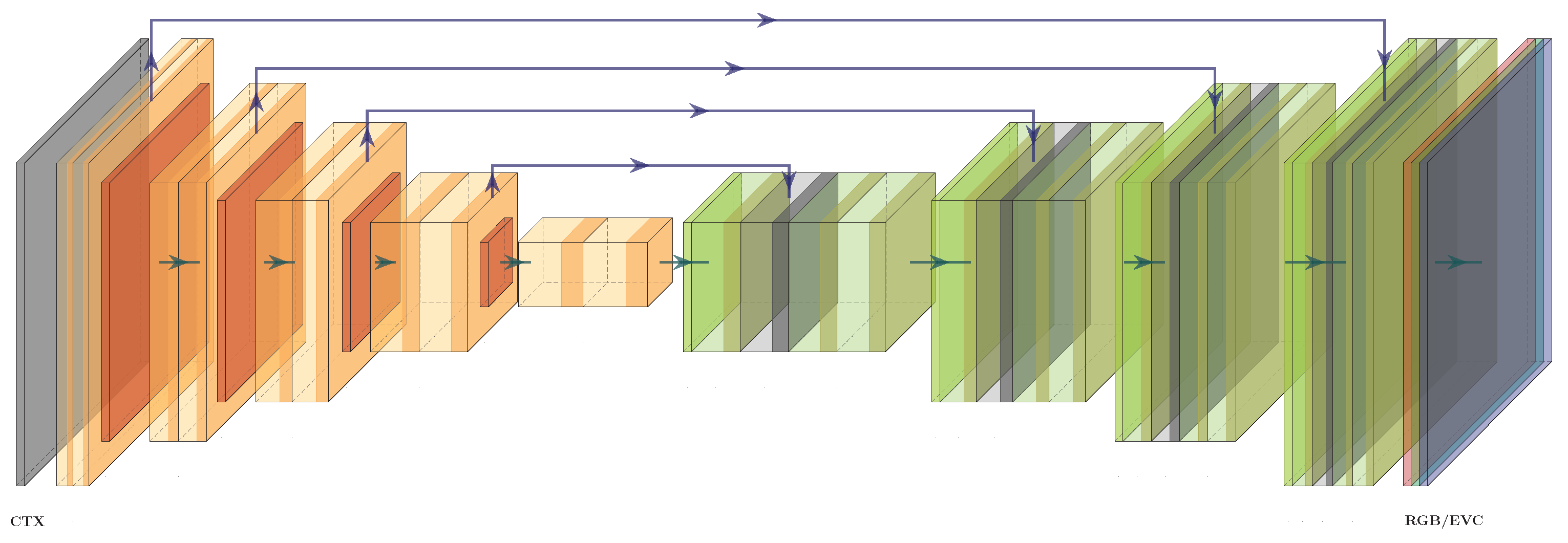
A regression approach serves as the baseline strategy, as it can be directly implemented. In this formulation, a segmentation model is given CTX images and is tasked to predict pixel-wise continuous spectral values. Due to memory constraints, training and evaluation are performed by processing smaller patches, which are cut out from original CTX images, instead of whole images. With this configuration, a monochromatic CTX patch is processed by a neural network, as shown in Figure 1, to produce a correspondingly sized multiband patch. This is achieved via a series of trained convolutional operations, pooling operations and non-linearities along an encoder and decoder path. We selected different semantic segmentation architectures as the building blocks of our approach and adopted them for the current task by utilizing a regression loss, such as root mean squared error, instead of a semantic segmentation loss. The majority of networks examined in this work exhibit an encoder–decoder structure, which is highlighted in Figure 1 using orange and green coloration. One of the most persistent modifications to this structure is U-Net’s skip connections, visualized as arrows in Figure 1, which start from encoder blocks and end in correspondingly sized decoder blocks, regardless of whether they are implemented as concatenations, additions or other operations and the way in which they are connected (cf. Section 2).
During training, the predicted multi-band patch is compared to a ground-truth CRISM patch depicting the same location. Within this work, outputs are usually constrained to three spectral bands that compose enhanced visible color (EVC) browse products. These three bands correspond to red, green and blue (RGB) color channels in later visualizations. A continuous regression loss provides a single-valued metric of how close the prediction is to the ground truth, with the goal of training to minimize the average of this loss across all training samples.
3.2. Classification
Transforming this task from regression to classification mainly involves the discretization of each CRISM pixel value into bins. Afterwards, the same architecture as before (cf. Figure 1) is used to predict bin indices, instead of actual values. Therefore, this approach is termed a classification approach, because the network is tasked to predict categories—the respective bin centers of a histogram—instead of continuous values, as discussed in the previous section. This procedure requires a suitable normalization to avoid the issues discussed in Appendix A.2. An interval of is chosen, which is divided into equidistant bins. The representative value of any bin is given by its center. Using this, each pixel value of every CRISM image is binned, with the target value now being the bin’s index and representing one of classes. The network is now required to output channels, with being the number of spectral bands, since every output value is predicted as a probability density. This constitutes additional computational effort compared to a regression approach, especially with an increased number of predicted spectral bands. In contrast, MDE and image colorization, as mentioned in Section 2, only require the prediction of one and two channels, respectively, making these tasks computationally easier. The network is trained using a per-pixel cross entropy loss by averaging the cross-entropy between each pixel’s predicted probability density and its corresponding ground-truth label.
Reconstructing an image from the network’s output can most simply be achieved by substituting each probability density with the bin’s representative value that has the highest probability. This, however, reduces the number of possible colors significantly and may lead to deviations in uncertain regions. A more robust and diverse color method is to calculate a weighted sum of the bin’s representative values using the probabilities as weights [35].
To avoid a network becoming biased towards certain classes when dealing with imbalanced datasets, class rebalancing methods are used in classification. The simplest way to implement such a method is to weight the loss of under-represented classes higher than overrepresented ones. A higher relative loss in these classes will result in a larger change in network parameters and should direct training towards a solution that is more accurate in predicting edge cases. For this application, an inverted Gauss distribution centered around the middle bin, and ranging from −1 to 1, is used as the weights. An exact formulation is shown in Equation (1), where the class index is used to calculate the class weights .
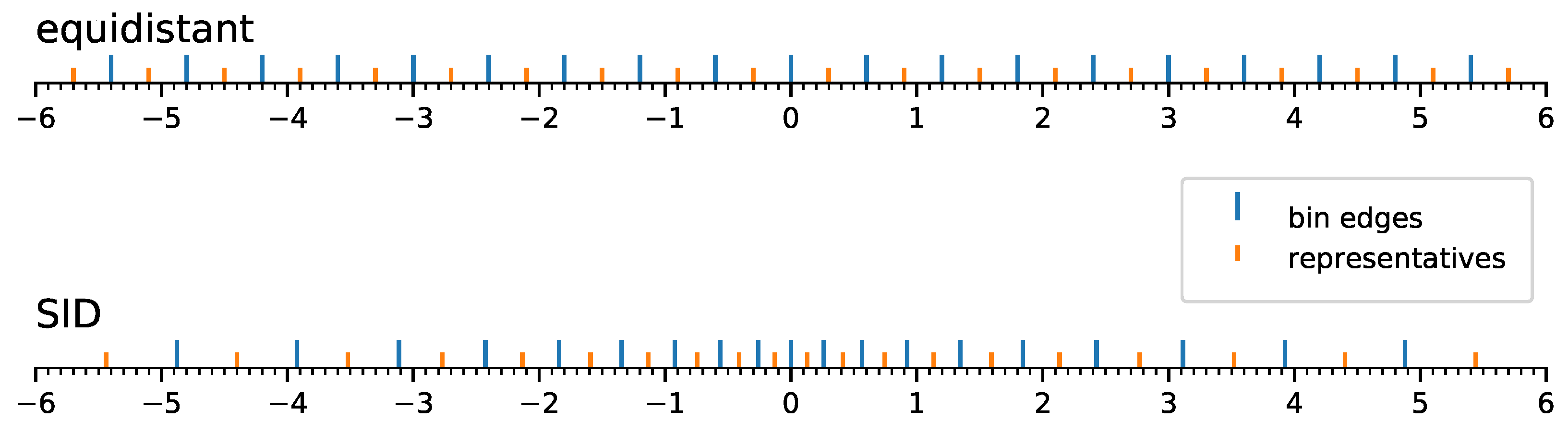
An alternative to rebalancing individual bins is to adapt the bin spacing. Spacing-increasing discretization (SID) is, for example, used by [21] in monocular depth estimation because a different importance is assigned to different regions of the output space. When predicting depth from an image, lower values are deemed to be more important than regions that are far away. In this task, due to the distribution of reflectance values and the normalization method, pixel values within an image are mostly clustered around zero and drop in frequency towards higher positive and negative values. SID can therefore be applied to decrease the size of bins close to the origin and increase their size going outward. This should reduce the discretization error in the majority of cases, but increase it in edge cases with extreme values. Figure 2 shows a visual representation of equidistant discretization compared with SID in the case of 20 bins. The two number lines demonstrate the range of values taken into account, the bin edges and their representative values. The final two bin edges are set to and .
3.3. Evaluation of Full Images
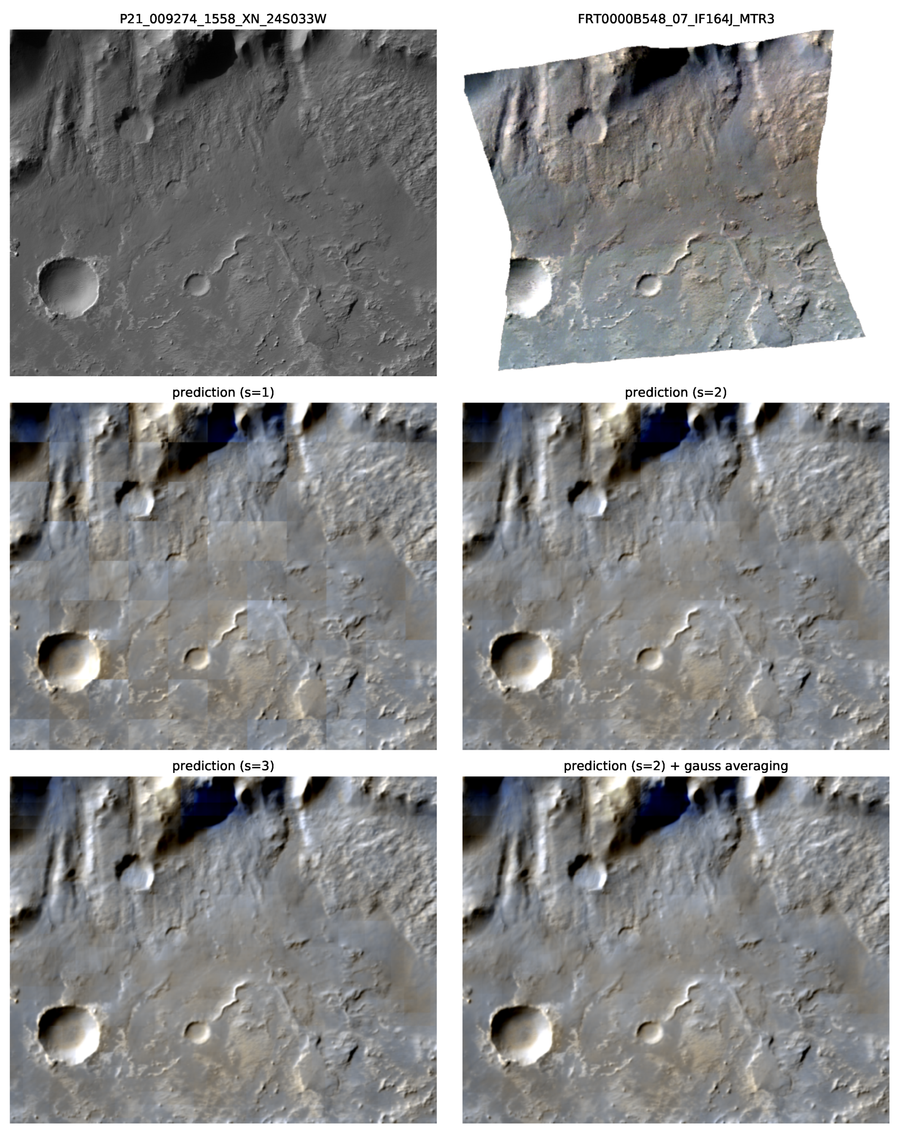
Using a patch-based method, larger CTX images can be processed in a sliding window manner with a constant stride of d, with d being the edge length of square patches. The image needs to be padded by d pixels on the bottom and right to fully evaluate these regions, unless the height and width of the CTX image are a multiple of d. A reflection padding that mirrors pixel values within the image prevents steep edges and therefore faulty predictions, resulting in cleaner boarders. Due to potential discontinuities at patch borders, which manifest as edges in a grad pattern, a smarter strategy is desirable. The adverse effect can be mitigated by reducing the stride to and averaging the outputs of overlapping regions. Doing this, however, requires as many patches to be processed. With increasing s, discontinuities become more numerous, but less apparent. Equation (2) shows how any given output pixel y is calculated using all of the N overlapping pixels of that same position via an arithmetic mean. Since the problem occurs at the edge of patches, a better averaging method can be utilized, where pixels further from a patch’s center are weighted less. In this case, a two-dimensional Gauss kernel is used as weights. The exact formulation is given in Equation (3), with and being the row and column pixel coordinates, while h and w are the height and width of the patch. To achieve the desired effect, both pixel coordinates are mapped to the interval , represented by and , which are used to calculate the weights .
4. Materials
In Section 4.1, an overview is given of the MRO’s two imaging instruments upon which this work is based, including their technical specifications and scientific objectives. The specific data products used in this work are subsequently named in Section 4.2 and their properties are discussed. Following this, various steps towards creating a suitable dataset are presented in Section 4.3. These include the acquisition and choice of data files, coregistration, sample selection, clipping and data normalization. In Section 4.4, specific data augmentation techniques seen as appropriate are discussed.
4.1. Imaging Instruments of the Mars Reconnaissance Orbiter
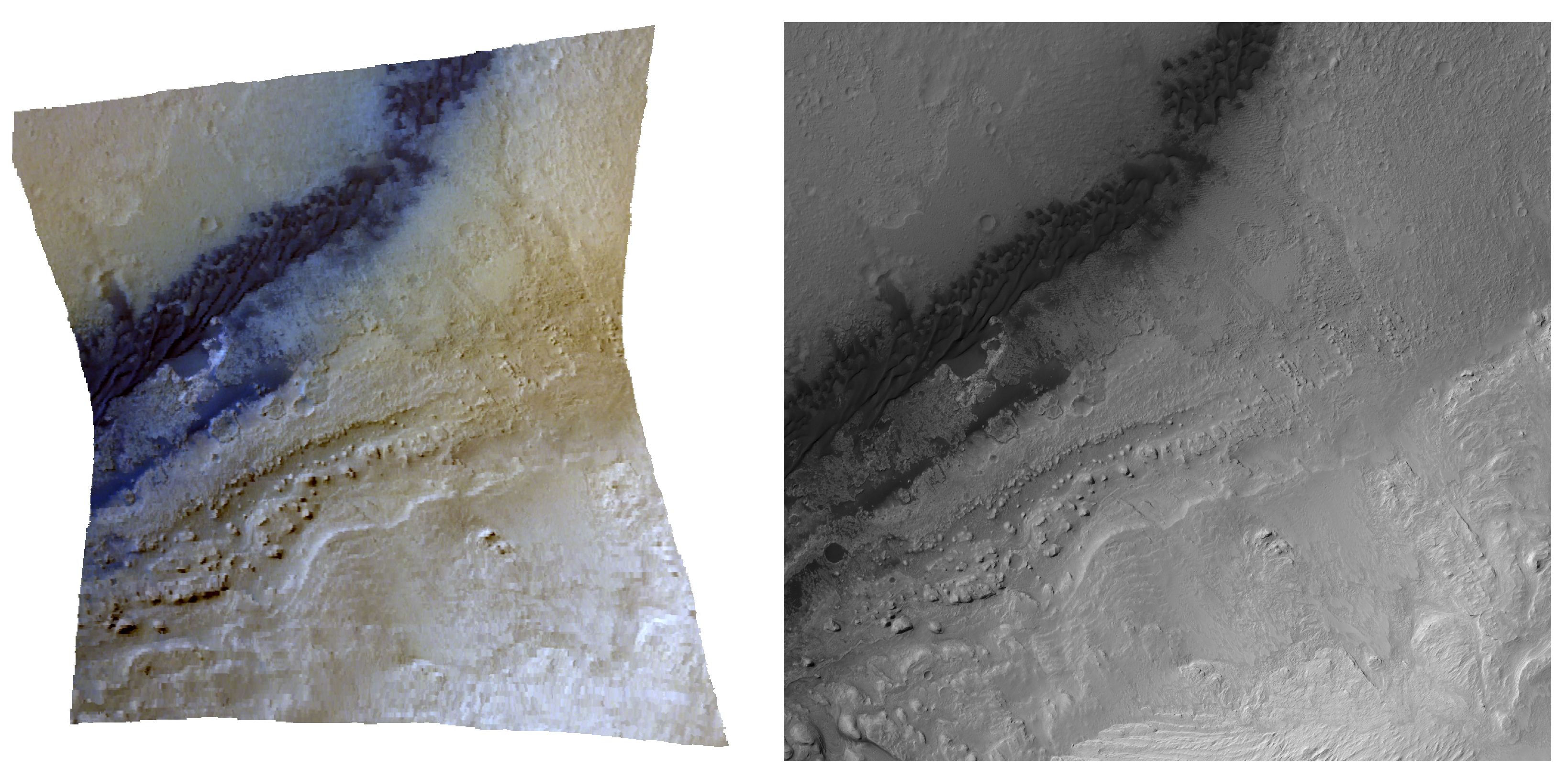
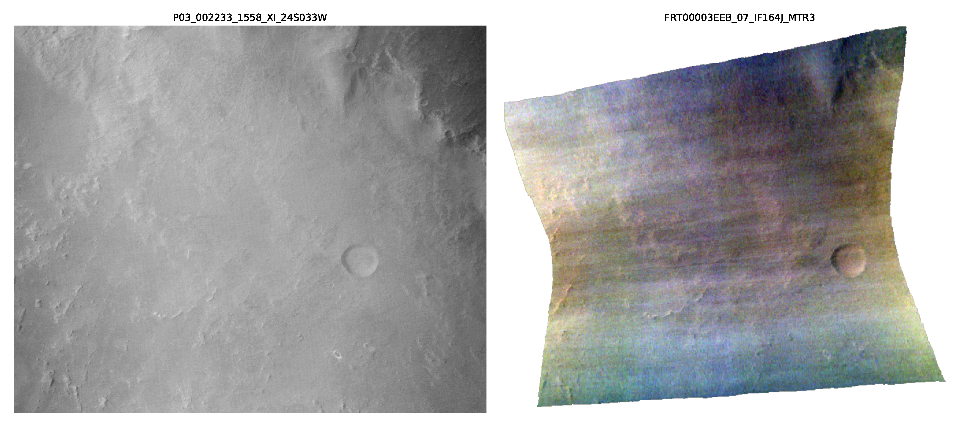
The MRO was launched on 12 August 2005 to study the geology and climate of Mars. Its science objectives include the observation of its present climate, search for aqueous activity, mapping and characterization of the Martian surface, and examination of potential future landing sites [1]. Among its many special-purpose instruments, the CTX and CRISM cameras are the subject of this work and, therefore, are discussed in the following two sections. Figure 3 shows an exemplary enhanced visible color (EVC) image of CRISM compared to a corresponding cut-out from CTX, in order to illustrate differences in appearance. CTX images, being only single-channel, are visualized as grayscale by mapping the reflectance values of shown scenes to the minimum and maximum brightnesses. Compared to this, EVC shows a composite of only three ( 592 , 533 , and 442 ) out of over 400 spectral channels.
4.1.1. CRISM
Images from the CRISM instrument are the primary focus of this work. Its gimbaled optical sensor unit can be operated in multispectral untargeted, or hyperspectral targeted mode. The untargeted mode allows the reconnaissance of large areas due to reduced spatial and spectral resolution in order to discover scientifically interesting locations. Such locations are then mapped with the full spatial resolution of 15 to 19 and full spectral resolution of 362 –3920 at per channel in targeted mode. CRISM’s mission objectives are to characterize the crustal mineralogy across the entire surface, to map the mineralogy of key areas and to measure spatial and seasonal variations in the atmosphere [2].
Hyperspectral imaging data, such as those captured by CRISM, are the basis of visible-near infrared reflectance spectroscopy. Each pixel represents a reflectance spectrum with characteristic absorption bands depending on the materials. These spectra are then compared to laboratory measurements to determine the mineralogical composition. The right-hand side of Figure 4 shows one such spectrum. In order to visually highlight or distinguish minerals within an image or scene, browse products are created. These are synthesized RGB color images, where each channel is assigned to a summary parameter, such as band depth or some other calculated measure of spectral variability, and afterwards stretched to a specific range. The previously mentioned spectrum is taken from a red region of the browse product displayed in the center of Figure 4, whose red channel is set to the BD1300 parameter, corresponding to iron olivine.
The simplest browse products, such as enhanced visible color (see Figure 3) or false color, are constructed by setting each RGB channel to one specific reflectance band. These browse products are visualized using a 3-sigma data stretch applied to each band (crism.jhuapl.edu/msllandingsites/browse/abtBrwPrd1.php, accessed on 24 January 2022). This means that the values of each individual channel i above and below are clipped to that boundary, with and being the mean and standard deviation of those values, respectively, and afterwards mapped to the minimum and maximum brightnesses.
4.1.2. CTX
The Context Camera’s primary function is to provide contextual information for other MRO instruments, by making simultaneous observations. It is also used to observe candidate landing sites and conduct investigations into the geologic, geomorphic, and meteorological processes on Mars. Owing to the 5064-pixel wide line array CCD and a 256 large DRAM, the pictures taken are 30 wide and up to 160 long, covering a much larger surface area than CRISM. These images are exclusively monochromatic, filtered through a bandpass ranging from 500 to 700. The spatial resolution is 6 /, making it around three times higher than CRISM [3].
CTX data have been used to create a seamless mosaic of Mars resampled to 5 / [36]. This allows the analysis of much larger regions by studying more localized observations made by other instruments and extrapolating these findings to outer areas. The instrument has further collected many stereo pairs, prompting the creation of digital elevation models that aid in quantitative analyses of Martian landforms [37].
4.2. Data Products and Properties
All CRISM images were acquired at the most recent, publicly available, calibration level, called Map-projected Targeted Reduced Data Record (MTRDR). Its joined visible/near-infrared plus infrared (VNIR-IR) full spectral image cube holds records in units of corrected I/F as 32-bit real numbers. I/F is the ratio of spectral radiance at the sensor and spectral irradiance of the Sun. The creation pipeline of this product type includes a series of standard spectral corrections and spatial transforms for the purposes of noise reduction and mitigation of data characteristics inherent to CRISM observations (https://ode.rsl.wustl.edu/mars/pagehelp/Content/Missions_Instruments/Mars%20Reconnaissance%20Orbiter/CRISM/CRISM%20Product%20Primer/CRISM%20Product%20Primer.htm, accessed on 24 January 2022). Out of this product suite, only Full Resolution Targeted (FRT) images were used, ensuring the maximum similarity to corresponding CTX data. Available CRISM FRT products were searched using the Orbital Data Explorer (ODE) REST API (https://oderest.rsl.wustl.edu/#ODERESTInterface). All relevant files related to FRT observations were downloaded from the Geosciences Node of NASA’s Planetary Data System (PDS) (https://pds-geosciences.wustl.edu/). Also contained in these products is a text table that lists wavelength information for the spectral image cube. After the removal of spectral channels with suspect radiometry during the creation pipeline, 489 bands with wavelengths ranging from 436.13 to 3896.76 remain.
At the time of writing, there exist a total of 9677 MTRDR CRISM products, with 6479 FRT among them. Older calibration levels such as Targeted Reduced Data Record (TRDR) include even more files, 1,754,260 in total. Having this many samples provides a great opportunity for large-scale deep learning applications, although the amount of data also presents a challenge. Each CRISM IMG file within the dataset measures at around 1 and more. The size of their corresponding and fully processed CTX images varies based on the height between around 200 and 2 or more, even though only a small cut-out is required in the end. Some CTX observations have the fortunate property of being closest in time to multiple CRISM observations, reducing the number of CTX images that need to be processed slightly.
Important to note for later discussions on data augmentation is the spacecraft’s orbit and its impact on images taken. The MRO is placed into a low and near-circular sun-synchronous Mars orbit with a mean local solar time of 3:10 PM to perform its remote sensing investigations [2]. This means that images captured by its instruments will have a similar angle of incidence, resulting in topological structures always being illuminated on the same side, while casting their shadow on the other [38]. This consistency is expected to be instrumental for a neural network’s decision-making process and should therefore be conserved.
4.3. Dataset Creation
Training a neural network benefits from a large amount of high-quality data [39]. The dataset used in this work is composed of multiple CRISM-CTX image pairs, as displayed in Figure 3, taken from a selection of locations on Mars. This section describes in detail the creation process, starting with location selection and data acquisition. Subsequently, the multitude of preprocessing steps are outlined, which include CTX image creation, coregistration, the extraction of patches and clipping. Finally, three data normalization methods are compared and discussed. These steps serve as basic requirements for creating a dataset that is suitable for machine learning.
4.3.1. Acquisition
Due to the large file sizes of CRISM FRT products and CTX images mentioned in Section 4.2, this work will focus on six locations and their respective CRISM observations. Table 1 lists these locations, their associated latitude–longitude bounding box that was searched for observations and the number of MTRDR products that are found within. A complete list of all CRISM images and their corresponding CTX images used along with additional information, such as the image set they are assigned to, can be found in Table A2, Table A3, Table A4, Table A5, Table A6 and Table A7.
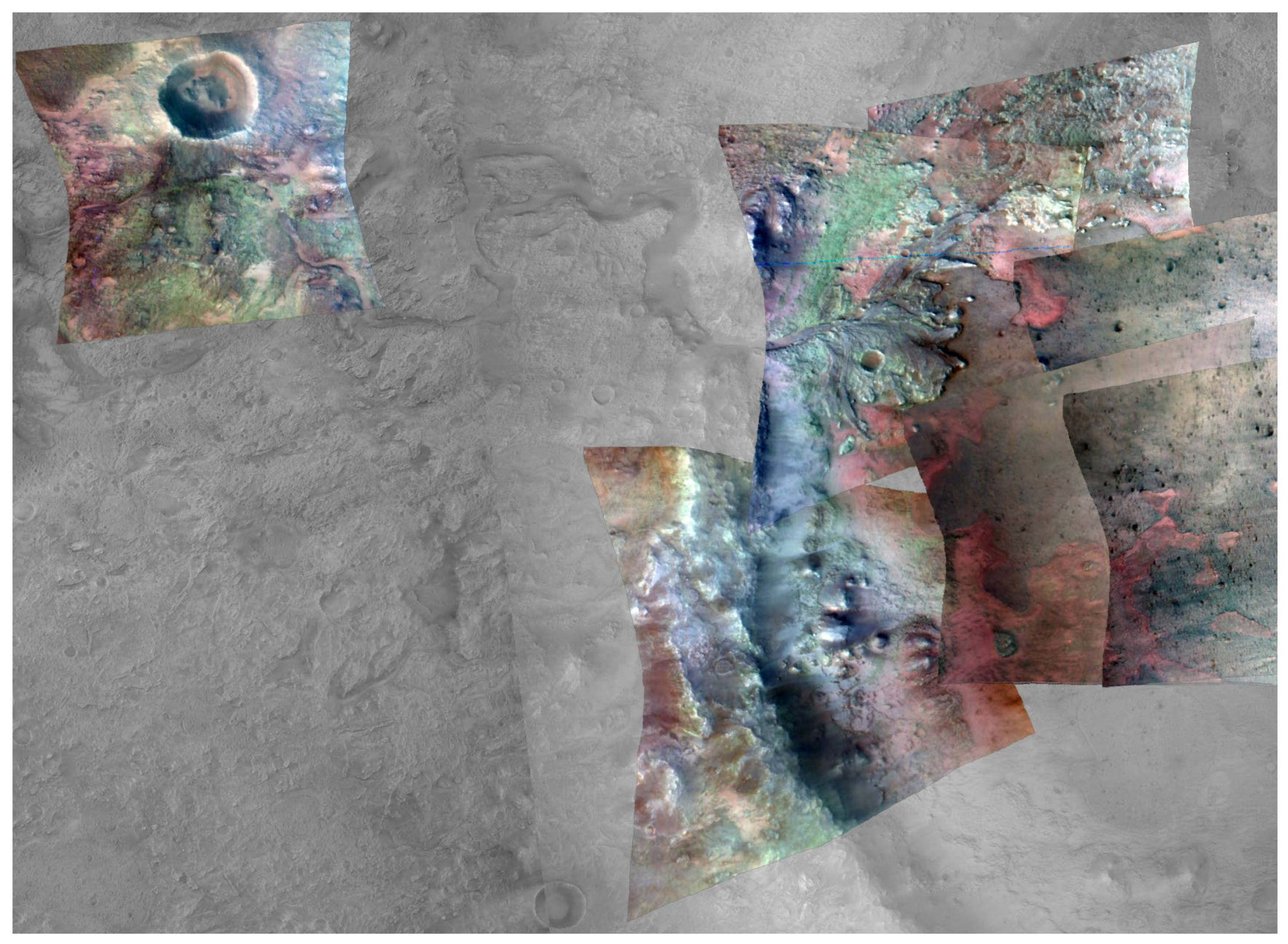
These areas are chosen because they are either previous landing sites, candidate landing sites or generally significant landmarks of Mars, and already have a large body of research due to their scientific interest. Bounding boxes were queried using the Orbital Data Explorer’s (ODE) REST API [40], and all FRT-MTRDRs within them are obtained. Another query was conducted for each CRISM image, retrieving all CTX observations which are fully contained in it in terms of latitude–longitude bounding boxes. Out of these, the one closest in creation time is chosen as its corresponding input. This was done in order to minimize the difference between these images, due to changes over time or seasons. Many but not all CRISM observations have a CTX image taken at the same time, which are marked as ride-along. The exact creation time differences in days between CRISM and CTX pairs are listen in the dt column of Table A2, Table A3, Table A4, Table A5, Table A6 and Table A7. Some CRISM images within the locations overlap, as is illustrated in Figure 5, which was taken into account for the evaluation process. The test and validation images used to evaluate the generalization capabilities of models were chosen such that they share minimal area with images within the training set. The separated observation on the left side of Figure 5, for example, would be chosen as a test image. This can be seen in the set affiliation column of Table A2, Table A3, Table A4, Table A5, Table A6 and Table A7 when considering the overlap column that shows the average percentage overlap of each CRISM image with all other CRISM images of that location. Only two images from each location belong to the test and validation sets to maximize the amount of data available for training. A validation set during training can reveal whether the model over- or under-fits. Finally, CRISM images that are deemed too noisy or contain large artifacts are omitted from the training set and marked with a dashed line. One such example along with its corresponding CTX cut-out is displayed in Figure 6.
4.4. Augmentation
Since the goal of this work is to accurately predict spectral bands, no changes to ground-truth CRISM pixel values such as brightness or gamma are considered. Furthermore, due to the consistency in the illumination direction mentioned in Section 4.2, vertical and horizontal flipping operations are not included. Such images never appear in the collection of CRISM files, and are therefore not useful training samples. One of the abilities a trained network should illustrate is to detect shaded regions and accurately determine their properties, which flipped samples would disrupt.
The augmentations examined in this work are random croppings or deletions of sections, rotation and zoom. Rotations are limited to a small interval, as to not significantly change the direction of illumination. The degree of rotation is randomly chosen from the interval . The height and width of cropped sections are independently taken from the interval , while the height and width of erased sections are taken from , with d denoting the side length of patches. Translational changes are not needed since the random way in which patches are cut out covers any possible location. Each training patch pair—consisting of CTX input image and CRISM ground truth—is given an equal probability of being left unchanged, rotated, cropped or having a section erased. The aforementioned augmentations are applied to both images equally. Invalid data regions created as a result of cropping, deletion and rotation are masked and not included in the loss calculation.
5. Results
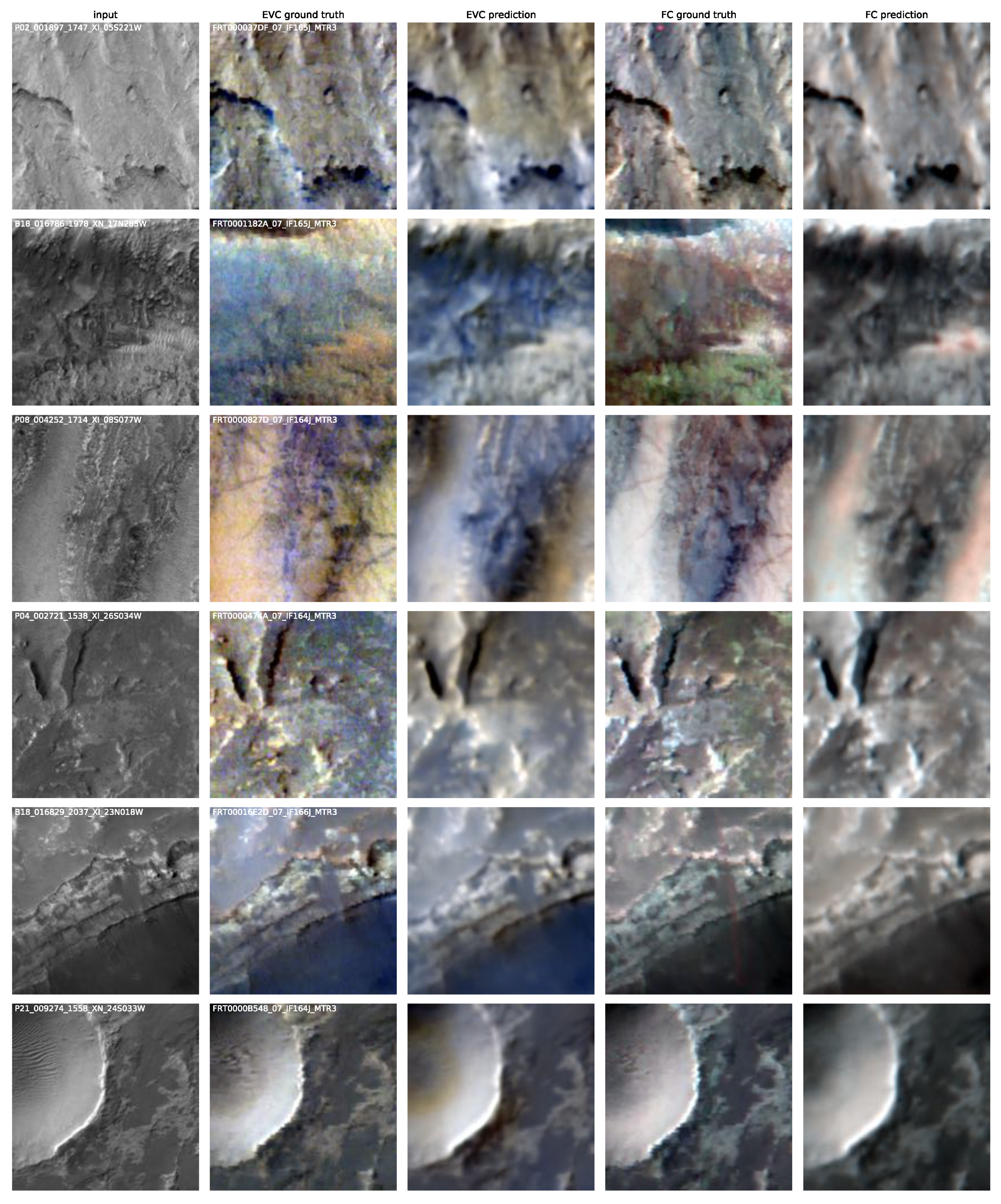
In this section, methods and tools that have been presented and created are applied, and their results are compared. Initially, the task is formulated as a pixel-wise regression problem. This formulation serves to establish a basic training configuration. Afterwards, the problem is reformulated as a pixel-wise classification of binned pixel values in Section 5.4.3 and compared to the basic configuration. Lastly, in Section 5.6, the best-performing model is used to assess the capabilities of a machine learning approach more generally and possible areas of application are suggested and demonstrated. For all experiments, the single-input channel from the CTX instrument is used to predict three CRISM channels. In the case of enhanced visible color (EVC) wavelengths 592 , 533 , and 442 are used. In the case of false color (FC) 2503 , 1500 , and 1080 are used (see Table A1).
5.1. Model Architecture
A comparison of different model architectures is the first experiment performed. This, however, requires the pre-selection of some parameters and methods for a training process to function. The following list lays out the base configuration used for each model.
- Number of training epochs: 360;
- Patch size: 256 by 256 ;
- Batch size: 16;
- Data normalization method: image-wise;
- Optimizer: Adam;
- Learning rate: ;
- Loss function: MSE.
The number of epochs and image-wise normalization are chosen based on prior experiments, while a batch size of 16 guarantees that each models fits into memory. The patch size and learning rate are common default values, whereas MSE and Adam are robust first choices.
Most of the compared models are taken from an implementation named Segmentation Models PyTorch (https://github.com/qubvel/segmentation_models.pytorch, accessed on 24 January 2022) (SMP), which provide a selection of architectures intended for image segmentation applications. Each architecture can be initialized with different encoders that are pre-trained on publicly available datasets. In this comparison, every architecture is initialized with the same ResNet18 (see Section 2) encoder pre-trained on ImageNet [41]. Two additional U-Nets are compared, a biomedical segmentation model created by [42] and another one used by [18] as a CGAN generator for image colorization.
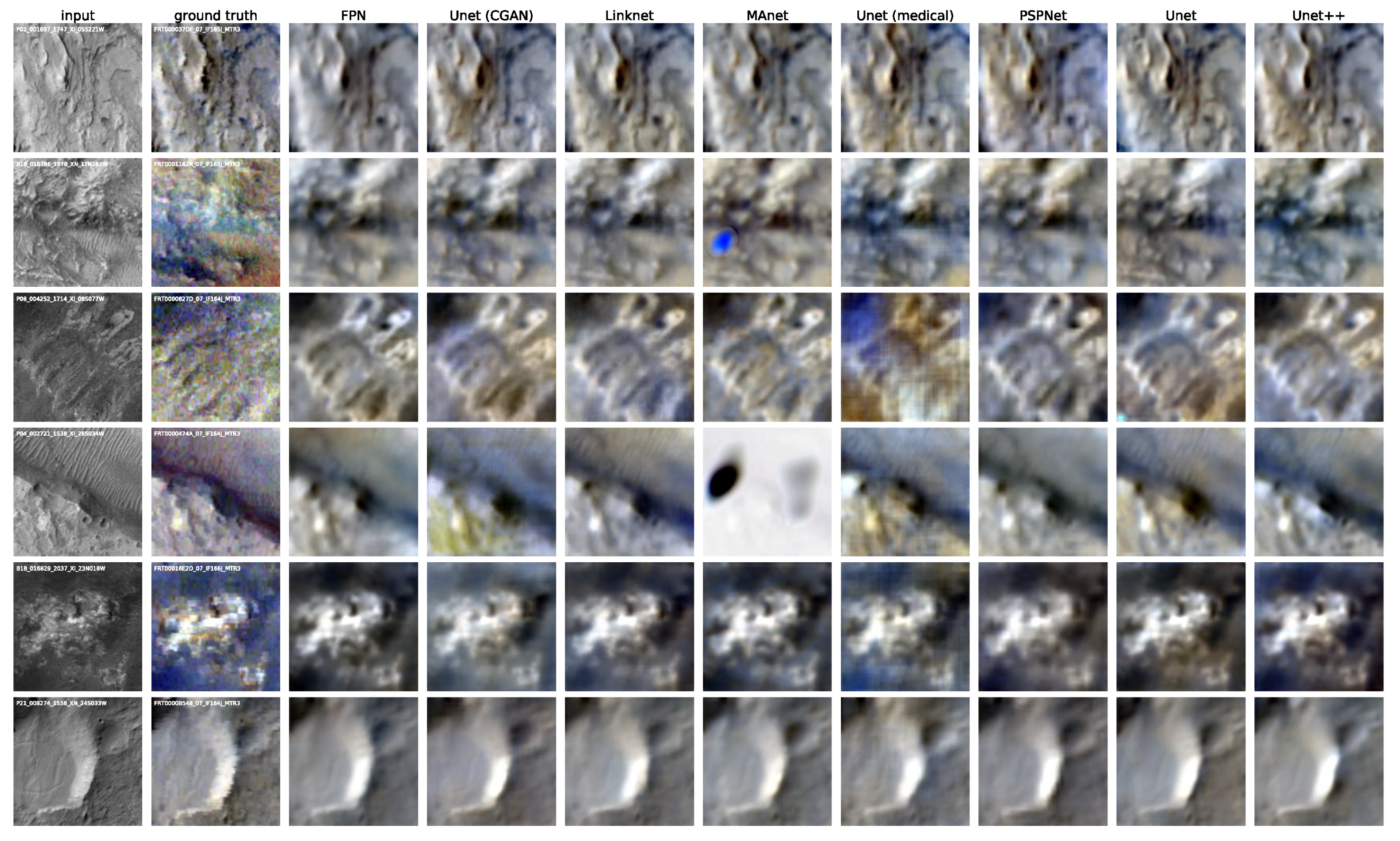
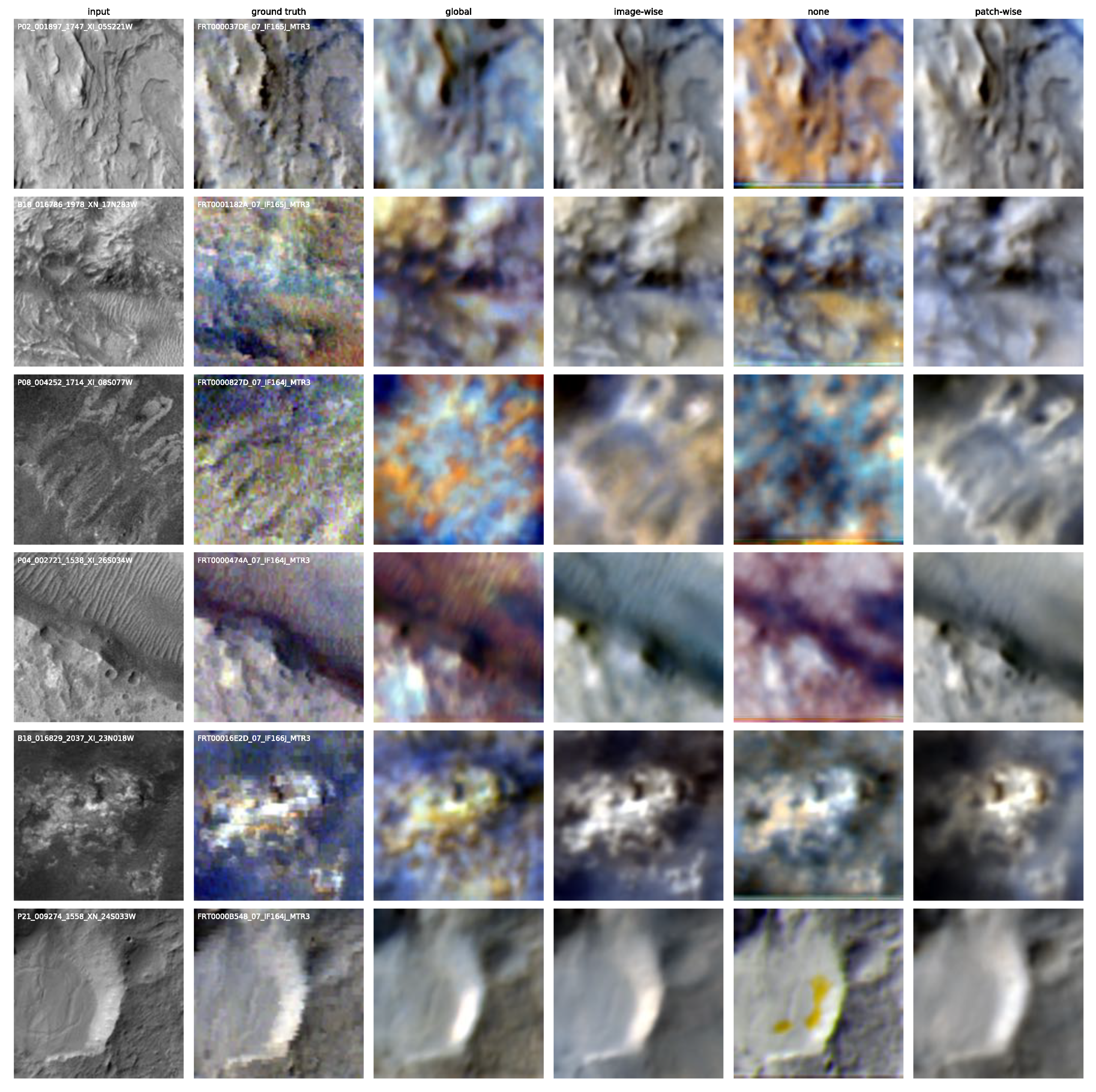
Figure 7 shows six input CTX and ground-truth CRISM patch pairs, one from each of the test images, with their file names in the top left corner. Every subsequent column displays the output of each compared model architecture when given the corresponding CTX patch as input after training. For visualization purposes, CRISM patches are displayed using a channel wise 3-sigma stretch. As mentioned in Section 4.3.1, not every CRISM image is taken at the same time as its CTX counterpart, meaning that in these cases the model output and ground-truth CRISM need to be compared with respect to the provided input. For a better assessment of the quality of the predictions, channel-wise histograms are presented in Figure 8. A comparison of measurable performance metrics is given in Table 2. They include three metrics—root mean squared error (RMSE), cosine similarity (Cosine), and Pearson correlation coefficient (PCC)—with the average loss of the final epoch over all training samples, the network’s number of trainable parameters, the maximum memory consumption during training, and the average training time per epoch.
The first observation of note is the difficulty faced when relying on regular regression losses when judging the performance of models employed in this task, as a result of artifacts, a lower resolution and the noisiness of CRISM samples compared to CTX. Even a hypothetical ideal output patch that is color accurate, sharp and noise-free would still result in an error compared to the ground truth. Quantifying the quality of unseen validation and test samples when non-global normalization methods are used is especially troubled. This is because values of input–output pixels depicting the same area can be different, depending on from which image or patch they are taken. A network could therefore correctly predict the hue of a given area, but with a wrong magnitude, still resulting in a high loss. A comparison of visual appearance is therefore prioritized.
For one, the test image pair of row three is exemplary of an especially noisy CRISM and CTX observation, as they are occasionally found within the dataset. With such CRISM patches as the ground truth, it is more difficult to judge the accuracy of predictions. Noisy CTX inputs, which can additionally contain large stripes such as artifacts, which can be faintly seen in Figure 6, further result in widely varying predictions of lower quality. Otherwise, immediately noticeable when examining the fourth row of patches is that the MAnet introduces large artifacts with extreme values, which is reflected in its high test loss. Since the remaining test losses are very similar and not correlated with the image quality or accuracy of outputs, test loss appears to be an insufficient performance metric in this case, due to the aforementioned challenges. Time and memory requirements vary significantly depending on the model architecture. Among the most time-consuming and memory-intensive models are the medical U-Net with its two-layered blocks at full resolution, the CGAN U-Net with its large size, and Unet++ with its complex skip connections. In general, all remaining SMP models exhibit a lower memory footprint and training time because of their shared ResNet18 encoder that uses a 3 × 3 pooling operation at the beginning of the model.
PSPNet, like some other segmentation networks, includes an upsampling operation at the end, making it unable to create sharp images. Other networks suffer from occasional striping artifacts, inaccurate colors, or desaturation, such as U-Net (medical), U-Net (CGAN) and FPN, respectively. Both Unet and Unet++ produce some of the most visually appealing images, although the Unet++ requires close to twice the memory and time due to its complexity. The regular Unet is therefore chosen. However, sometimes it produces artifacts at corners, as can be seen in the third row. Since the problem occurs at the edge, it can be speculated that the standard zero-padding procedure causes this issue. Switching to a reflection-based padding removes these artifacts, as can be seen when comparing the bottom left corner of the third row of the Unet column of Figure 7 with the third row of the resnet18 column of Figure 9.
5.2. Encoders
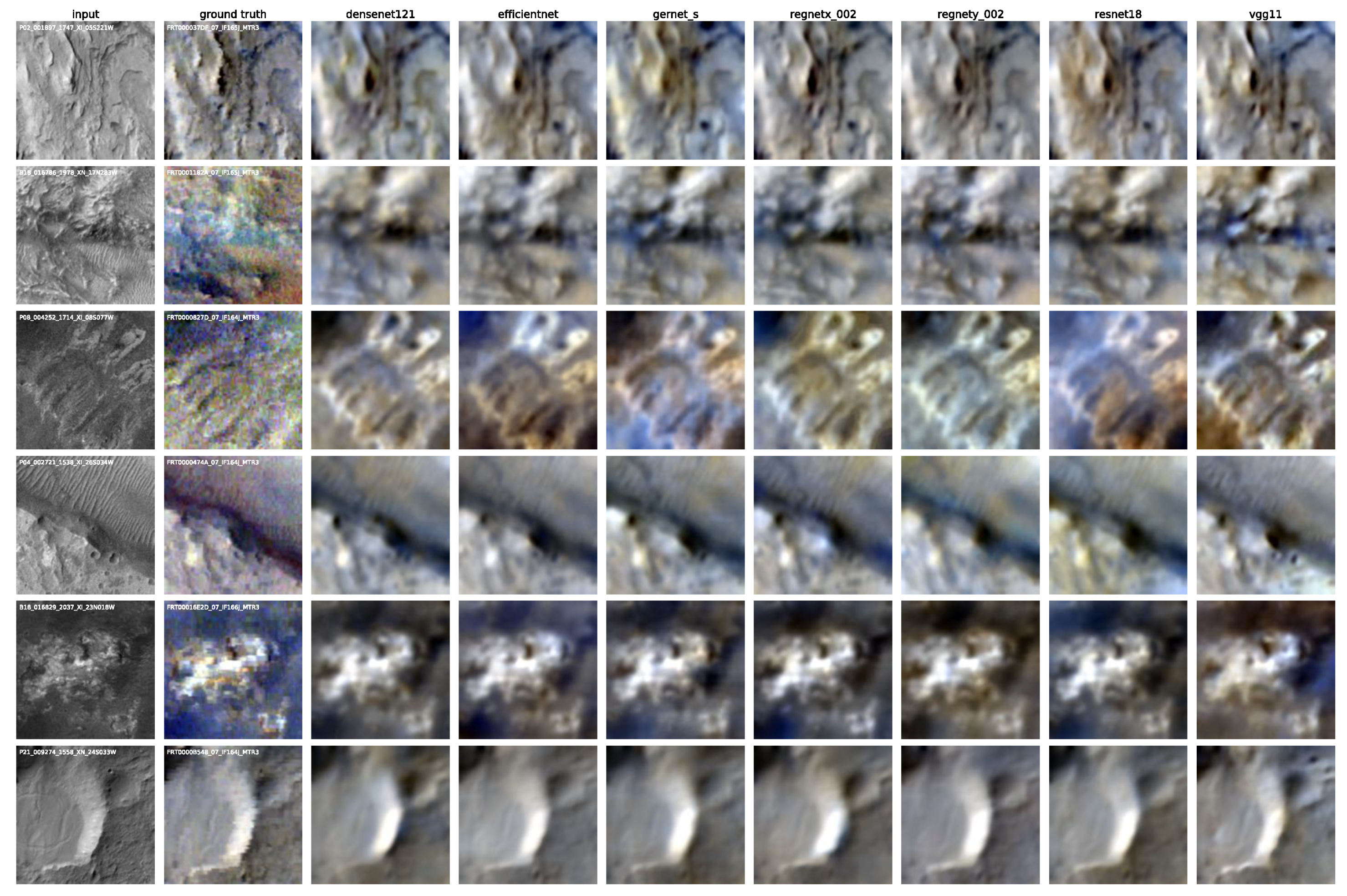
With Unet being chosen, different encoders can be compared in the same way. Out of the encoders provided by SMP, a selection of prominent architectures with a similar number of parameters were taken. Scaled-up versions of these models exist, but the smallest configuration was used for this comparison. Each of them was pre-trained on ImageNet. In the same manner as before, the results can be seen in Figure 9 and Table 3.
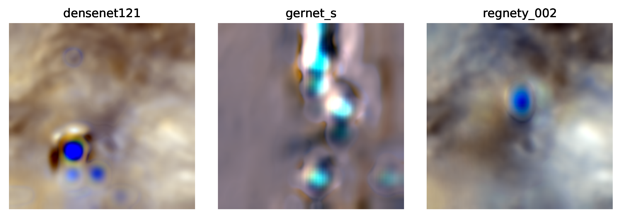
There is far less difference in appearance between encoders compared to models. A particularly low train loss of the VGG11 encoder stands out, although this is neither noticeably reflected in the appearance of the predicted patches nor in the metrics. One problem that emerged during training is that some models showed a diverging behavior. GerNet, DenseNet, and both RegNets show spikes in validation loss that far exceed the usual values. These models sometimes produce artifacts with extreme values in their outputs, which happen to not be present in Figure 9. Three exemplary artifacts from each of the models are shown in Figure 10. Such divergences could potentially be solved with regularization techniques such as weight decay by lowering the learning rate or they could stem from some incompatibility between the model architecture and this problem formulation. Despite these issues, the patches predicted by these models that do not suffer from artifacts are still comparable to any of the other outputs. The remaining encoders, ResNet, EfficientNet and VGG, produce similar images, but EfficientNet was chosen for further tests, as it is also among the lowest in parameter count, giving it more room for expansion.
5.3. Evaluation of Full Images
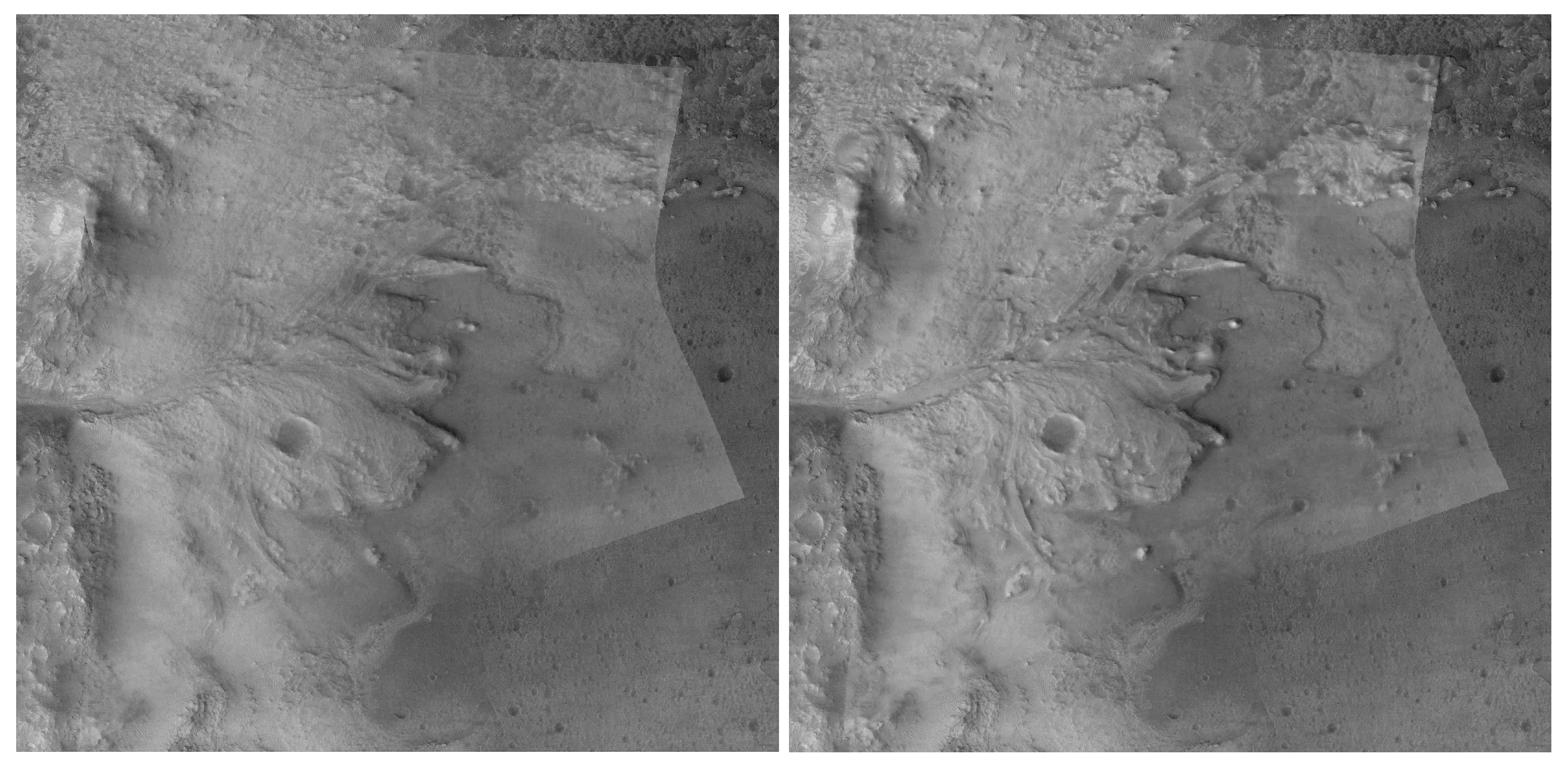
Figure 11 depicts an entire input CTX cut-out alongside its ground-truth CRISM image in the top row, together with the current network’s prediction in the mid-left image, generated via the aforementioned method. The quantitative results are presented in Table 4.
The Gaussian averaging strategy performs best in providing visually seamless results when comparing the lower two images. Even though the left image requires as many patches to be processed, the right image still appears slightly more or just as seamless, showing the importance of weighting pixels towards the edge less. By examining the accuracy of this full image prediction, it can be said that hue and saturation are consistently plausible for images from the Eberswalde crater and are comparable with the ground truth. Out of the six locations that are used for training, each of which exhibits a different kind of color scheme, the model is able to predict an accurate set of colors for this unseen image. Only two spots at the top edge are colored overly blue. The separation between a more brown half at the top and a mostly turquoise region at the bottom as seen in the ground truth is also lost in the prediction. This can be attributed to insufficient context being provided to the model because of too-small patches, resulting in an inability to capture larger trends. Another less likely cause is the time difference of 16 days between the CTX and CRISM observations, which can mean that the reflectance properties during the CTX’s recording are different from what is seen in its corresponding CRISM image. On average, the time difference between each image pair is 29 days (cf. Table A2, Table A3, Table A4, Table A5, Table A6 and Table A7).
5.4. Ablation Study
After selecting the Unet with an EfficientNet Encoder, we conducted a set of ablation studies to test how incremental changes to the normalization method, the loss function, and adding additional input data affect the metrics. The results are summarized in Table 5 and discussed in the following sections.
5.4.1. Normalization Methods
Using a Unet with an EfficientNet encoder, the three data normalization methods in Appendix A.2 are compared. With the network being fixed, the batch size is increased to 32, while all other parameters remain. Since the magnitude of pixel values is vastly different between comparands, a direct comparison of losses is not possible. Lower values result in lower losses and vice versa. The only remaining metric that is different across normalization methods is the training time, where a patch-wise normalization necessitates on the fly calculations that can not be performed prior, increasing the training time slightly. The mean and standard deviation of each CRISM and CTX channel across the entire dataset that are used for global normalization can be seen in Table A1. Predictions of six patches are shown in Figure 12.
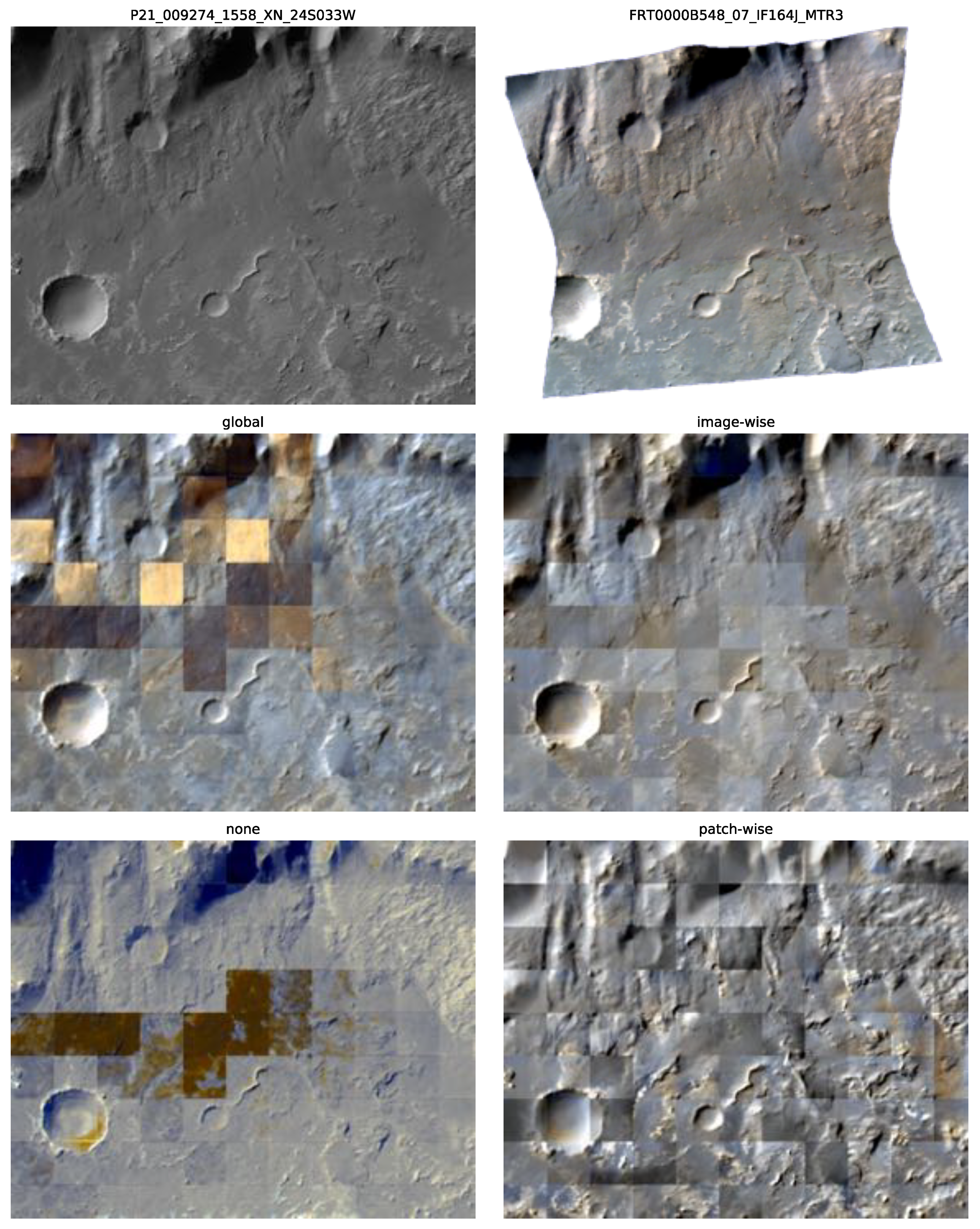
Un-normalized data are confirmed to be unsuitable for this application. The network creates unfitting colors, as shown in the first row, line artifacts at the bottom of patches and miscolored spots in the last row. This is reflected in the first row of Table 5, which shows the second highest RMSE and the lowest PCC and COSS. Globally transformed data result in more stable and accurate outputs. Obvious miscolorizations and artifacts in the first and last rows are remedied with this method. However, the issue of pixel value distributions of CRISM bands being different orders of magnitude and often constrained to small intervals still proves challenging for the model. The metrics in the second row of Table 5 coincide with these issues, as this method results in the highest RMSE and second lowest PCC. Both globally and non-normalized data seem to be particularly problematic in combination with noisy input and output pairs, as shown in the third row, where predictions appear especially blurry and spotted. Image-wise and patch-wise normalizations produce the most consistent results in comparison, with both being quite similar. Patch-wise outputs are sometimes more color-accurate, such as when predicting the blue area in the bottom left quantile of the second row patch. It also appears sharper in some instances, as in the bottom left of the fourth row. These two methods are listed in the third and fourth rows in Table 5, and score much better than the first two methods discussed. Major differences, however, emerge if an evaluation of entire CTX cut-outs is attempted, which are shown in Figure 13.
Without normalization, not much colorization or processing is applied to the input image and some patches produce widely spanning artifacts. Global normalization yields much more plausibly colored results, but some patches stand out again as being miscolored. Both these results indicate an unstable training process and a non-robust model, which drastically changes its output if the input shows a slightly different region. With patch-wise normalization, each individual output appears plausible, but it is not directly possible to reassemble the image. With each patch occupying a similar range of values, discontinuities are strongly apparent, as would be the case when putting together ground-truth patches. In this predicted reassembly, some patches appear desaturated and gray, while others exhibit a broad range of colors that are not fitting with those given areas. Compared to this, an image-wise normalization allows the creation of a coherent overall image, since ground-truth patches now form a continuum across each image. The more favorable distribution of pixel values compared to global normalization also improved the robustness of the network, hence why this method was chosen for further comparisons.
5.4.2. Digital Elevation Model
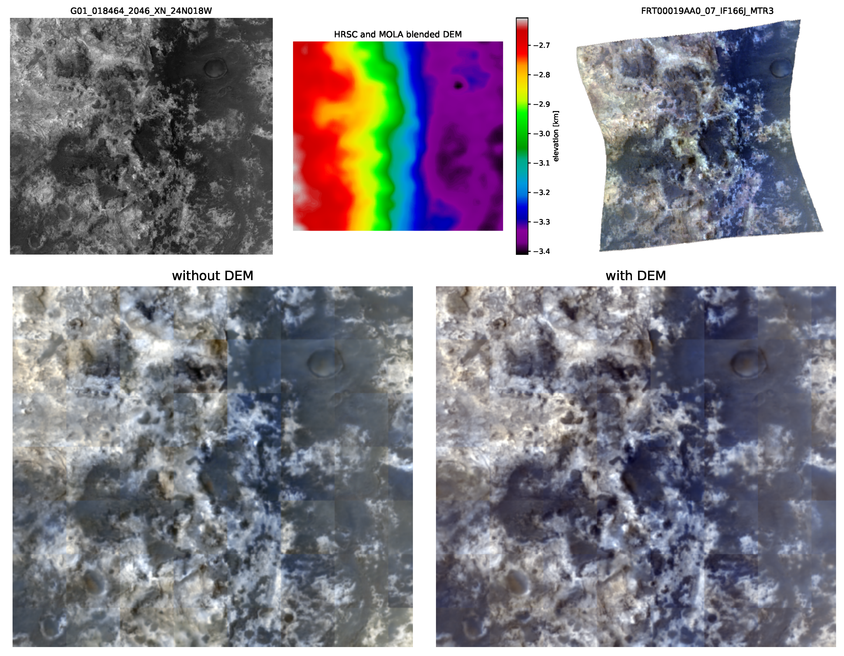
Elevation data can improve network performance if used in training as an additional cue. In cases where certain minerals correlate with the characteristic topology, pixel-wise elevation data of sufficient resolution can be helpful to a network in identifying them. At a smaller scale, positive or negative gradients along the axis of illumination determine whether a region is shaded or illuminated. If given enough context, then the detection of hills and valleys can also factor into a prediction. For this test, the HRSC and MOLA blended digital elevation model (DEM) by [44] with a resolution of 200 / is used, which is far lower than the CTX resolution. This can therefore only benefit the prediction of larger landmarks and regions. Each CTX-CRISM image pair’s bounding box is used to cut out that region from the global DEM and the resulting image is added to the dataset. The elevation values are given in meters and range within the thousands, making them unusable without normalization. For this, an image-wise normalization analogously to CTX is used. The input is now made up of CTX patches that are channel-wise concatenated with their corresponding DEM patches. In accordance with this, the number of input channels of the network is changed to two.
To examine the impact of including DEMs in the input at a larger scale, a comparison of full CTX predictions was conducted, specifically of Mawrth Vallis’ validation pair depicted in Figure 14. The top row shows the input CTX and un-normalized DEM cut-out on the left, and ground-truth CRISM on the right. This pair was chosen because the DEM exhibits a clear horizontal gradation, sectioning the ground truth into two distinct halves. This information seems to have benefited the model that utilized it during training, as seen in the bottom right image, which is closer to ground truth in terms of color accuracy. In contrast, the models trained without that information in the bottom left predict colors less accurately and create an overall less coherent image.
5.4.3. Classification
The goal of this section is to determine whether reformulating the problem as a classification task achieves better results (see Section 3.2). With this formulation, the model is tasked with assigning pixel-wise probabilities to discrete spectral values in each spectral band. Ground-truth CRISM reflectance values are normalized on an image-wise basis and afterwards assigned to equidistant bins within the interval . The various additional steps such as discretization, the prediction of more channels and output reconstruction make this approach more computationally expensive than regression. Having shown the overall best performance in the previous section, a U-Net with an EfficientNet-B0 encoder is used again to predict EVC spectral bands. To obtain the desired output, the final convolutional layer’s number of output channels is changed to , with being the number of spectral bands predicted. Its output tensor of shape is subsequently reshaped to in order to simplify the loss calculation and image reconstruction. H and W, in this case, are the height and width of the patches used.
Number of Bins
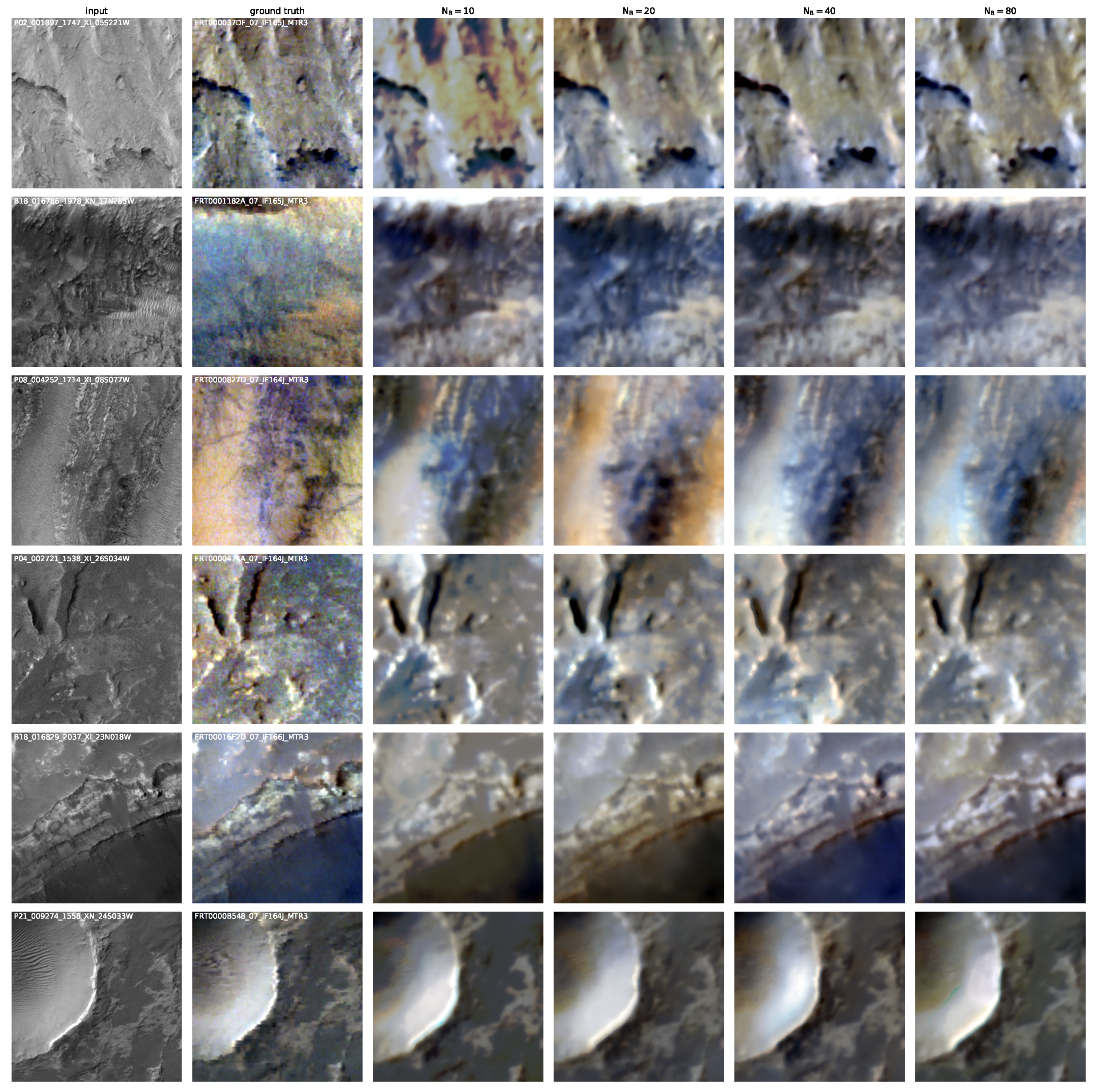
The first and most fundamental parameter to determine is the number of bins . A small number of bins results in fewer possible colors and larger quantization errors, while more bins requires additional computational effort and diminishes the advantage of discretization. The network is trained with four different bin counts and a constant batch size of 10. The resulting predictions of test patches are shown in Figure 15, when outputs are reconstructed using a weighted sum, as described in Section 3.2. The according metrics are listed in Table 6.
Judging the quality and accuracy of predictions in Figure 15, bins counts of 20 or 40 produce some of the better images, for example, in the second and third rows of and in the fifth row of . Ten bins are not sufficient to produce detailed results and 80 bins may be too many as more artifacts arise, such as the turquoise spot in the last row. This classification approach in general has shown to carry the risk of producing artifacts like this, which were not present in the regression approach. Examining test and train loss in Table 6 shows how more bins leads to higher losses, which is expected since the same prediction with more classes results in a higher cross-entropy loss. As a result of this, a judgement based on the cross-entropy loss is not possible in this comparison. Another noticeable trend is the increased demand of memory and time with more bins, because the final convolutional layer is required to output more channels. Even though the resulting increase in the number of parameters is very small, these weights are used to convolve many more full-resolution feature channels, which takes longer and requires more memory. Based on the quality of outputs and ease of computation, 20 bins were chosen for further comparisons.
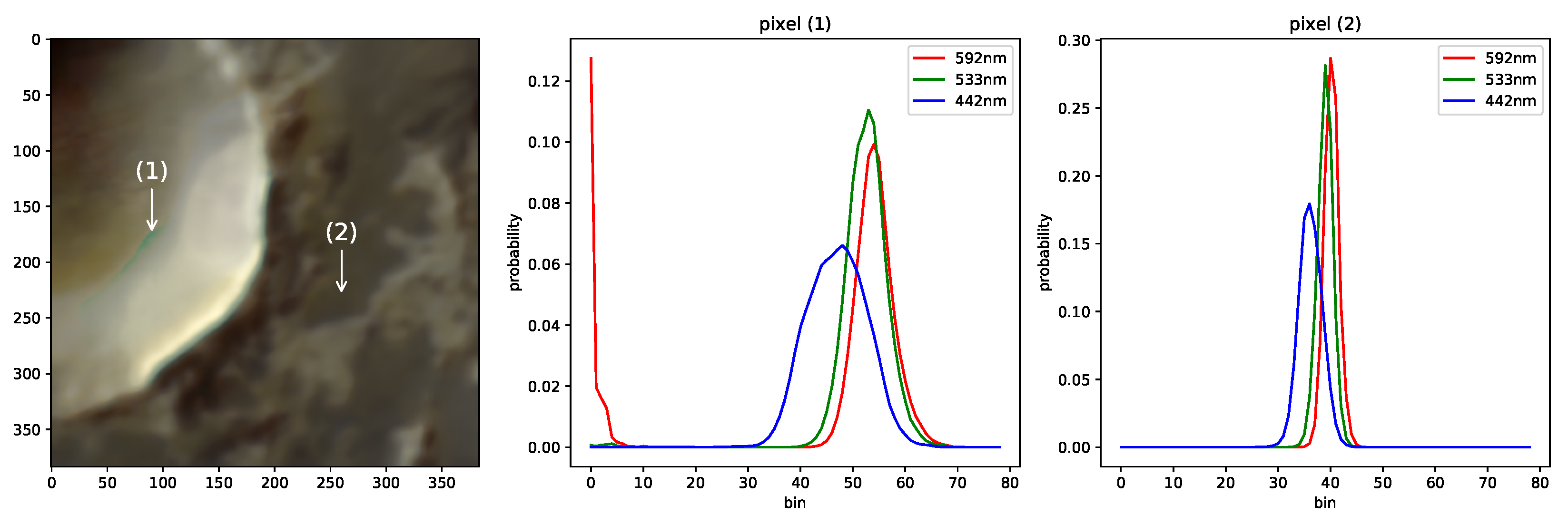
An advantage of this approach is that a measure of confidence is provided for each prediction. If the predicted probability density displays a single sharp peak, it can be said to be confident. A broad peak or multiple maxima conversely indicate uncertainty and are a hint for faulty predictions. Both cases are illustrated in Figure 16, where the bottom right prediction from Figure 15 is shown again on the left without a 3-sigma stretch. Two pixels are marked, (1) taken from a region within an artifact and (2) being an accurate prediction. Their predicted probability densities of each channel across bins are displayed to the right. Pixel (1) exhibits broader peaks in each channel and two maxima within the 592 channel, with the one at bin zero being clearly faulty and distorting the results no matter the used reconstruction method. The peaks of pixel (2), conversely, are sharper, which corresponds to more confident, and in this case accurate, predictions.
Loss Modification
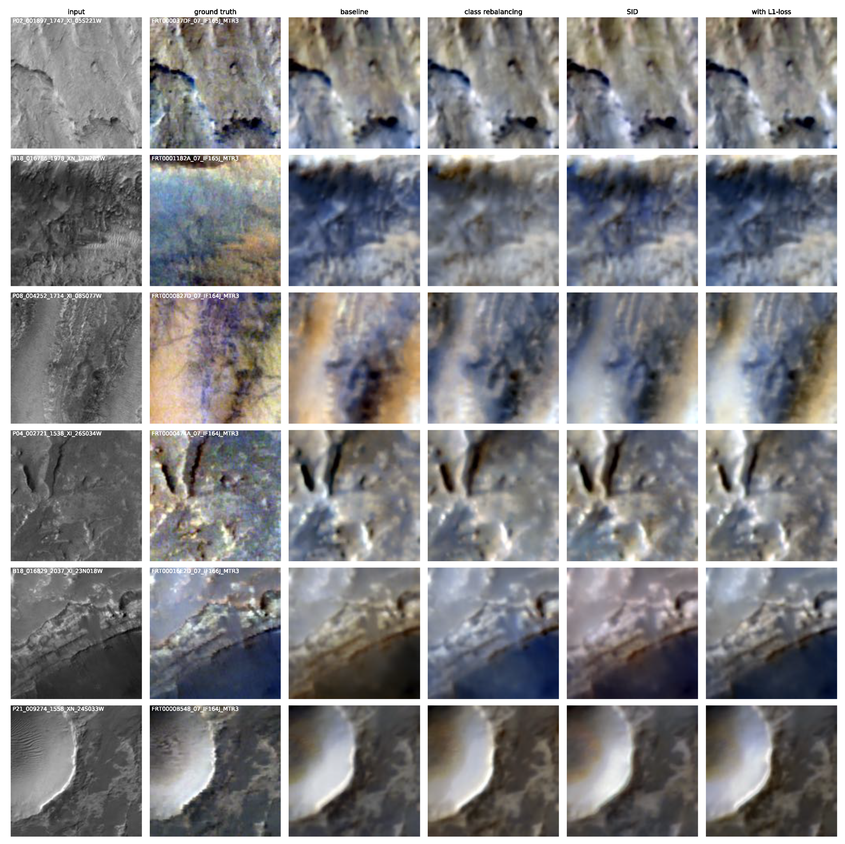
Additionally, we examined three modifications or additions to the problem formulation, which were used to address the shortcomings of the classification approach or offer improvements in general. Some of these are found within the literature, as mentioned in Section 2, and are adapted to this task. An overview of six test patches and the baseline model’s predictions with 20 bins is presented in Figure 17, which is compared to the model’s output if any of the modifications are enabled.
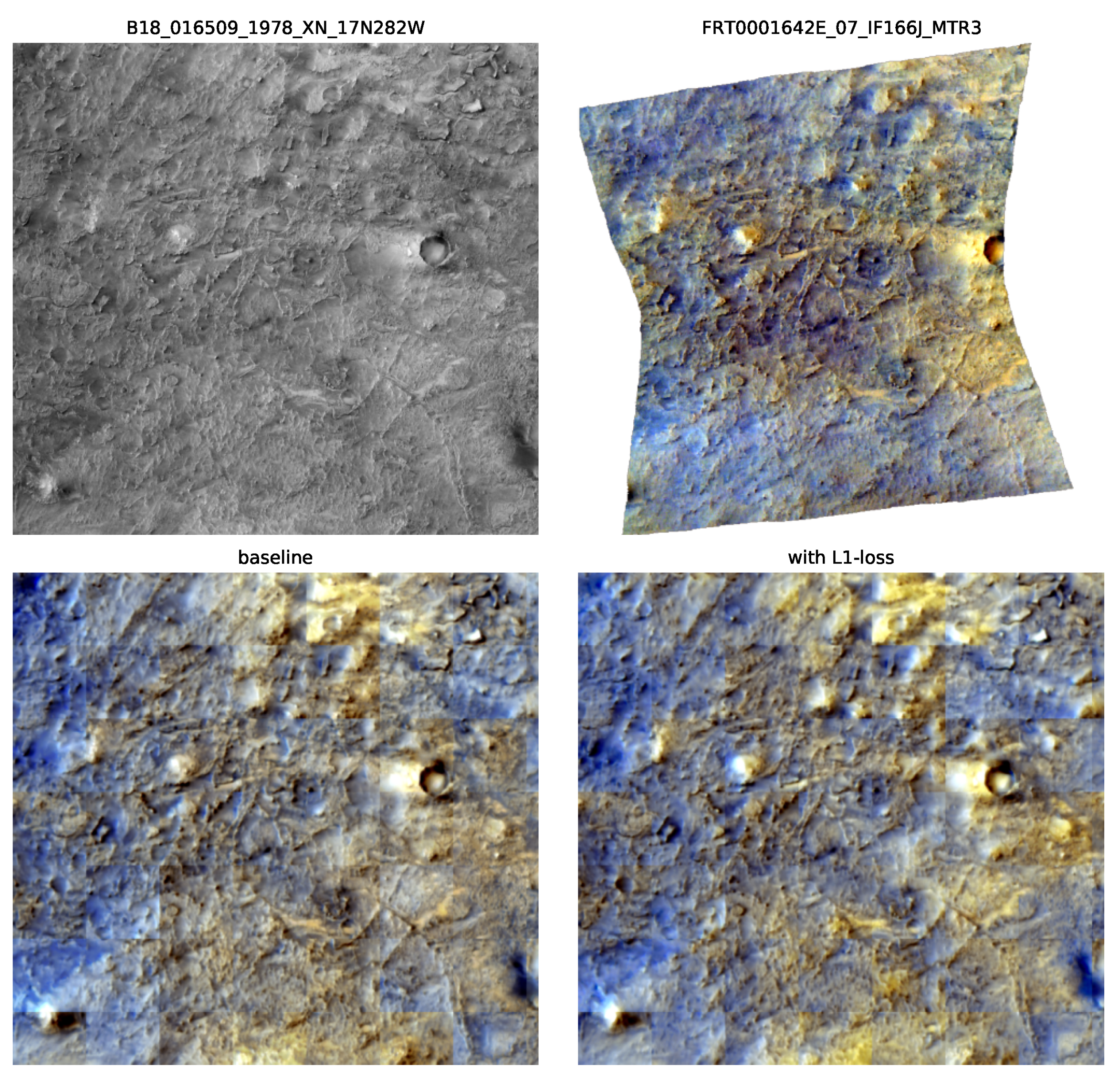
Regular cross-entropy loss does not take into account the distance of a wrong prediction from the ground truth. Only when the bell curve of predicted probabilities, as seen in the right plot in Figure 16, enters the correct bin does the loss measurably decrease with lower distance. One way to increase the loss of predictions that stray further from the ground truth is to introduce a regression loss component, where the absolute difference between the predicted value at the highest probability and ground truth value is additionally back-propagated. This is equivalent to reconstructing the network’s output using the argmax method and calculating the MAE between it and the ground-truth image. Due to the difference in magnitude between both types of losses, MAE is weighted by 0.9 and cross-entropy is weighted by 0.1 to arrive at similar scales, after which both are summed and back-propagated. In the last column of Figure 17, it is shown that there is not much difference between the model that utilizes this addition compared to the baseline model, except the superior colorization of the fifth patch. Examining larger areas, however, reveals some improvements, as is shown in Figure 18. This figure depicts the validation image of the Jezero crater and both model’s predictions. The model with a MAE loss component produces a more colorful image, especially in the yellow regions. Further, features such as the brown streak going from the center left to the top right and the crater’s wind streak are predicted more accurately.
Spacing-Increasing Discretization
Whether this technique reduces the quantization loss in practice can be tested by evaluating the MAE between ground-truth CRISM samples and predicted samples reconstructed via the argmax method. Doing this for one pass of the training set and comparing the model with and without SID reveals that the MAE drops from 0.32 to 0.3 if SID is used, a decrease of 6%. This shows that utilizing a SID slightly reduces the difference between predicted discrete and ground-truth continuous values.
5.5. False Color Prediction
Up to this point, only channels that make up enhanced visible color (EVC) browse products were predicted, which lie within the visible spectrum. This section examines the prediction of false color (FC) channels, situated in the infrared part of the spectrum. The three exact bands that constitute this browse product are 2503 nm, 1500 nm and 1080 , which correspond to red, green and blue color channels, respectively. Figure 19 shows six EVC test patches and predictions made by a model that is only trained on them. Two additional columns on the right show the same patches in FC, one being the ground truth and the other being predictions made by the same type of model trained only on FC channels. The patch size in this and following comparisons is increased to 384 by 384 pixels, meaning that different regions within each of the six test images are shown. This figure shows that learning a mapping between CTX and FC bands provides additional challenges compared to EVC. The general trend of blue, gray and pink shades in specific areas such as dunes in the third patch or the general appearance of the last patch is predicted adequately. Some areas, however, such as the green region of the second patch that indicates the presence of clay or potentially carbonates [45], is lost in the prediction. This is likely due to an imbalance in the dataset, because such green sections are almost exclusively found within the Jezero crater subset. These deviations from the norm are more localized and rare, which makes the mapping between CTX and CRISM’s infrared reflectance harder to learn. CRISM channels within the visible spectrum in comparison tend to exhibit wide spanning and clearer tendencies towards certain colors, such as the dark blue dunes or general beige terrain in Figure 3. The network may also be too small or unsuited to learn the features necessary for making a nuanced prediction such as this possible. A larger and potentially more balanced dataset, as well as a more powerful machine learning model, would presumably be better able to accurately predict such features.
5.6. Assessment of Capabilities and Applications
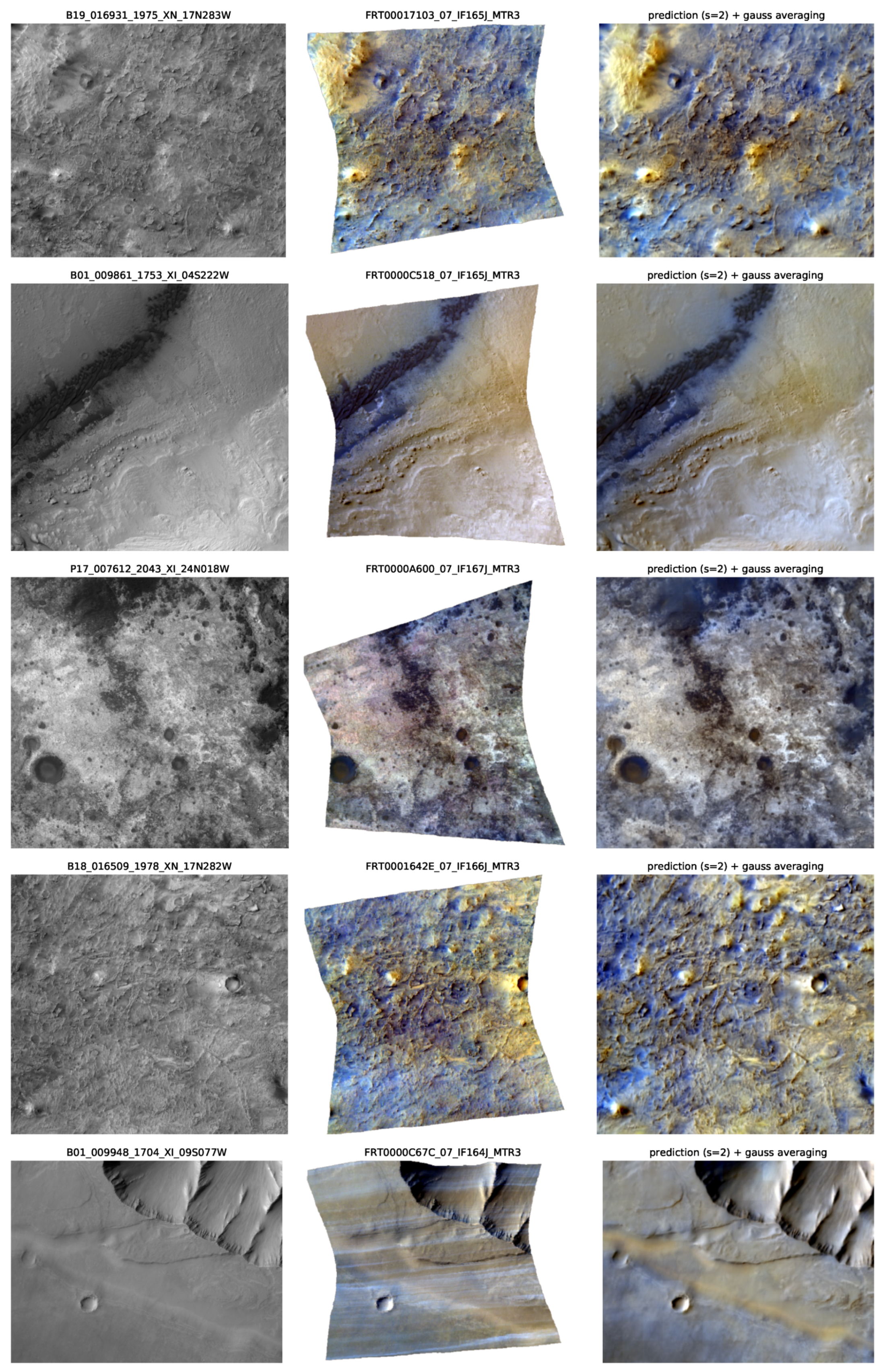
Concluding this chapter, a general assessment of the machine learning model’s capabilities is provided. Images from the training set and unseen images were evaluated to determine what factors are required for high-quality predictions and generalization abilities. Quantitative results are presented in Table 7. The final two examples show the restoration of a faulty CRISM observation and the evaluation of entire CTX images as possible areas of application. For this evaluation, the training configuration from Section 5.5 with rotational augmentation from Section 4.4 was used. It was trained for 500 epochs with a reduced learning rate of to obtain the following results.
Examining the predictions made by the model on CTX images that it was trained on, it can be seen that the model’s capacity is sufficient to memorize most of the training data. As long as the input and ground truth training data are of high quality, meaning minimally noisy and devoid of artifacts, reconstructions of these images are consistently accurate. The top two images in Figure 20 show the evaluation of two training images, which are very close to the ground truth and exhibit a promising continuation beyond the regions where CRISM data are available. Therefore, no over-fitting is observed in these cases, and predictions are more accurate the nearer they are to training locations. Inaccuracies arise when lower-quality data are used for training, and when the model is tasked to predict outputs that are infrequent within the dataset and only constitute a minor deviation from the norm. This second aspect is illustrated in the third image of Figure 20, which shows an overall very accurate reconstruction of an image from the training set, with plausible predictions beyond borders. However, the pink hue towards the top left is not captured in the prediction, as it is a less frequent deviation within the dataset. This same problem is observed more clearly in the prediction of false color bands.
The evaluation of unseen CTX images that have not been trained on and that share little to no area with the training set revealed the generalization capabilities to be adequate in most cases. Figure 20 shows one such example from the validation set, where the predicted color scheme is plausible throughout and the image quality is high. This second characteristic is naturally reliant on high-quality inputs, while the first characteristic requires enough similar data to be trained on. Because there exists at least one training image pair in Figure 20 that exhibits the same type of terrain and mineralogy, a plausible prediction can be made.
In Figure 21, we present two examples from the test set. Although variations in color are obvious, the resulting metrics presented in Table 7 show similar values to those from the training set. The proposed approach is thus able to generalize the spectral characteristics learned from the training set on unseen data.
One possible area of application that can be shown using the present dataset is the restoration of a faulty CRISM observation, as is presented in Figure 20. It can be seen how the CRISM image contains bright-blue horizontal striping artifacts that span the entire image. Since the input CTX image is faultless and the model is trained on data from that location, a prediction can be made. While it is difficult to verify the accuracy of this prediction, some aspects such as the central beige dunes and the blue-tinted bottom left region appear reasonable.
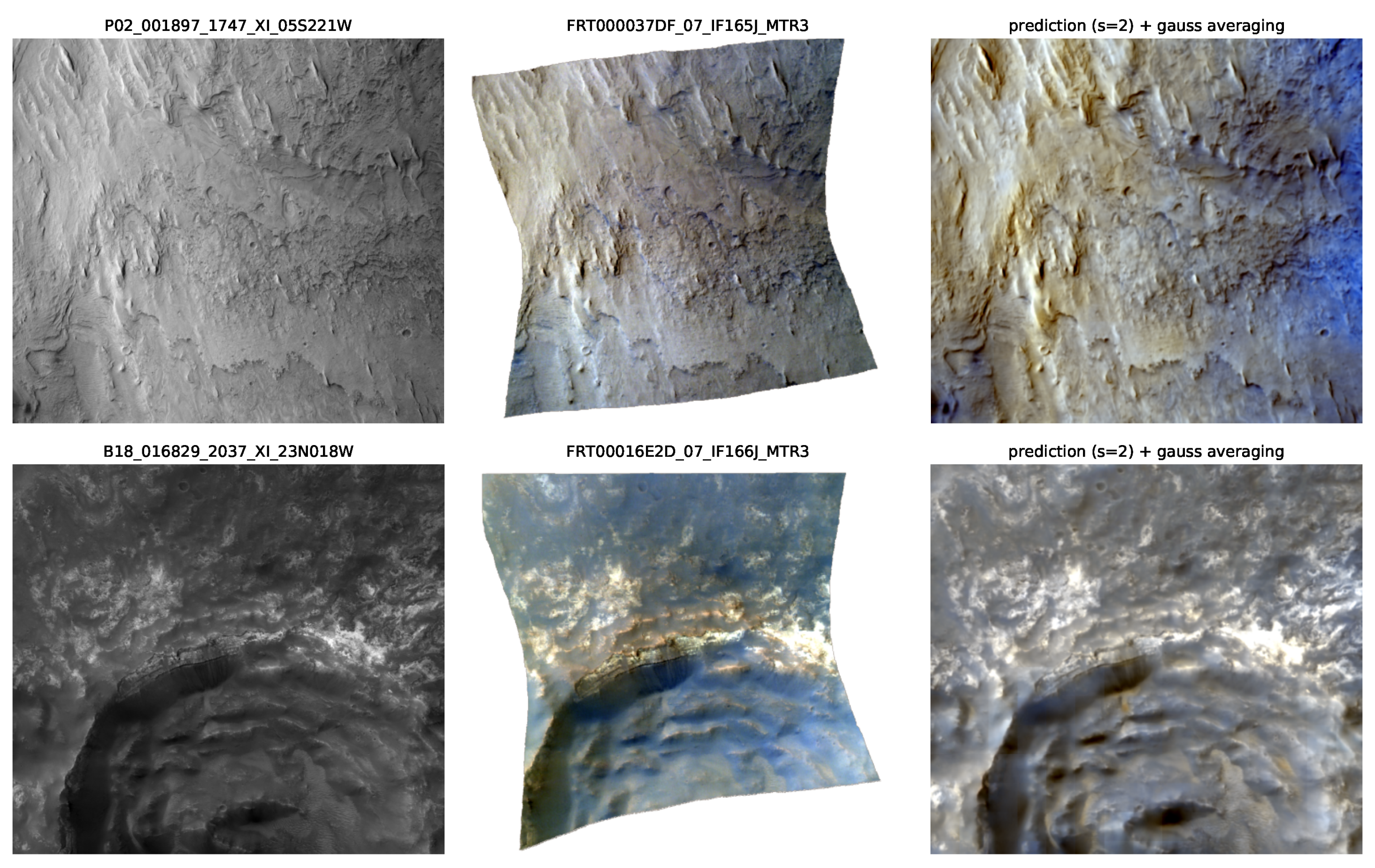
Finally, the evaluation of entire CTX images can now be attempted, instead of the much smaller cut-outs that have been examined and trained on thus far. The CTX image is normalized as a whole, which changes the pixel values compared to the image-wise normalized cut-outs that are used for training. A global normalization in comparison would preserve the same values. A successful prediction of a full CTX image is shown in Figure 22. Depending on the surface character of CTX, outputs are colored in accordance with images provided during training, as can be seen when comparing with first and the last but one row in Figure 20. These results show that plausible EVC images of large areas can be created within regions where high-quality training data are provided.
6. Discussion
Within the context of this work, it was found that common segmentation networks are capable of learning a generalizing mapping between CTX and CRISM reflectance within the visible spectrum. The capacity of models is sufficient to memorize training samples, while predictions beyond areas with CRISM data continue accurately. Unseen areas can be evaluated plausibly if high-quality training data of similar mineralogy were provided. Extending this task to the prediction of infrared channels yielded inferior results, due to the localized spectral variability. Upscaled networks and more data of under-represented features are likely required to obtain superior infrared predictions.
Regarding data normalization, it was observed that scaling each image and channel individually results in the most accurate and robust predictions, which also form a continuum across each image. In contrast, the normalization of each individual patch does not allow for a direct reassembly of an image, while patches normalized via global statistics remain constrained to unfavorable intervals and exhibit biases in certain spectral bands. With an image-wise normalization, however, it is not possible to apply an inverse transformation to obtain original reflectance values in areas where none are already available. A consequences of this is the inability to calculate the spectral parameters of most browse products in the usual way. For this reason, another normalization method or method of predicting spectral reflectance that preserves the ability to regain original values needs to be developed.
When comparing the machine learning methods examined in this work, it was found that posing the problem as a regression task in which square patches are predicted performs best overall. Reformulating the problem as a classification of binned spectral reflectance did not improve the quality of outputs, while increasing the demand on time and memory. Some functionality can be gained from these approaches, such as providing a measure of confidence when predicting probability densities across bins. Further research into classification methods is required if these approaches are to be used.
7. Conclusions
This work investigated the potential of machine learning approaches to predict pixel-wise CRISM spectral reflectance from CTX images. In pursuit of this, a dataset of 67 CRISM-CTX image pairs from six locations was created, and the methodologies of data acquisition, co-registration, extraction of patches, clipping, normalization and possible data augmentation methods were detailed. Various common machine learning approaches used in similar fields of study were presented and adjusted to this task. A pixel-wise regression approach that utilizes segmentation networks was the most extensively examined configuration. Different popular model architectures, encoders, and data normalization methods were compared to obtain a best-performing baseline configuration. Upon the baseline, various modifications and additions to the training process were tested. Performance was mainly judged on the basis of visual appearance, which includes color accuracy, consistency, sharpness and potential artifacts. This method was prioritized due to the difficulty of relying on losses when evaluating lower-quality and individually normalized image pairs. Metrics of quality, such as average training or test losses, and measures of computational effort, such as training duration and GPU memory requirements, were also considered. The beneficial and detrimental aspects of different configurations and techniques were discussed and hypotheses for successes and failures were provided. On the basis of these results, a classification approach was tested, in which continuous spectral reflectance is binned and pixel-wise probability densities across bins are predicted. Number of bins, methods of output reconstruction and other modifications or additions to the training process were tested and compared. Finally, the evaluation of entire CTX observations was performed, which constitutes one of the possible areas of application which were discussed. An extended dataset is likely to help with many of the shortcomings experienced in this work. A robust and automated pipeline for the acquisition, re-projection and coregistration of CRISM and CTX images can be used to create a larger dataset that is either focused on a specific location or is representative of the entire Martian surface. With more samples that contain rare deviations from the norm, predictions could be made more accurate. Alternatively, methods that emphasize these deviations during training may be explored. Finally, the prediction of all spectral bands that targeted CRISM observations provided can be attempted. Utilizing the similarity between and continuity along spectral bands can aid in this regard.
Author Contributions
Conceptualization, S.S. and T.W.; methodology, S.S. and T.W.; software, S.S.; validation, S.S. and T.W.; formal analysis, S.S.; investigation, S.S.; resources, S.S.; data curation, S.S.; writing—original draft preparation, S.S. and T.W.; writing—review and editing, T.W. and C.W.; visualization, S.S. and T.W.; supervision, T.W.; project administration, C.W.; funding acquisition, T.W. and C.W. All authors have read and agreed to the published version of the manuscript.
Funding
This work has been funded by the Deutsche Forschungsgemeinschaft (DFG, German Research Foundation)—Project number 269661170.
Data Availability Statement
The CTX images are available from https://pds-imaging.jpl.nasa.gov/data/marsreconnaissanceorbiter/ctx/ (accessed on 14 June 2022) and the CRISM MTRDR data are available from https://oderest.rsl.wustl.edu/ (accessed on 14 June 2022). The dataset used in this work is available at https://doi.org/10.5281/zenodo.6855065.
Conflicts of Interest
The authors declare no conflict of interest.
Appendix A. Dataset Preparation
Appendix A.1. Preprocessing
While CRISM MTRDR images were used as is, CTX images were created using an ISIS3 [46] pipeline. Raw IMG-files in Experiment Data Record (EDR) format were taken from the Planetary Data System (PDS) Imaging Node (https://pds-imaging.jpl.nasa.gov/, accessed on 26 January 2022). These were then converted to the ISIS3 image format, after which the following processing steps were run: the initialization of Spacecraft and Planetary ephemeredes, Instrument C-matrix and Event (SPICE) kernel data, radiometric calibration, the removal of vertical striping and finally the map-projection of the image.
The pixel-wise prediction of spectral information from grayscale necessitates a perfect match of input and ground-truth images. Shifts between input and ground-truth images can, in the case of edges, for example, result in high losses despite correct predictions and disrupt convergence during training. The coregistration of CRISM and CTX images was conducted by firstly re-projecting the CRISM MTRDR into the coordinate reference system of its corresponding CTX cube, using rasterio’s (https://github.com/mapbox/rasterio, accessed on 24 January 2022) virtual warping. To save time and reduce the size of the dataset, only bands which were used for later prediction were re-projected. These include all channels associated with the assembly of EVC and false color (FC) browse products as described by [45], whose wavelengths are listed in Table A1.

Table A1.
Wavelength, mean and standard deviation of each CRISM and CTX channel examined in this work.
Table A1.
Wavelength, mean and standard deviation of each CRISM and CTX channel examined in this work.
| Channel | Wavelength [nm] | Mean | Std |
|---|---|---|---|
| EVC (R) | 592 | 1.706 × 10⁻¹ | 3.596 × 10⁻² |
| EVC (G) | 533 | 1.080 × 10⁻¹ | 1.788 × 10⁻² |
| EVC (B) | 442 | 6.185 × 10⁻² | 7.651 × 10⁻³ |
| FC (R) | 2503 | 2.070 × 10⁻¹ | 6.476 × 10⁻² |
| FC (G) | 1500 | 2.106 × 10⁻¹ | 6.158 × 10⁻² |
| FC (B) | 1080 | 1.994 × 10⁻¹ | 5.927 × 10⁻² |
| CTX | 9.386 × 10⁻² | 3.062 × 10⁻² |
It is a known issue, however, that even within the same coordinate systems, CRISM and CTX images do not line up perfectly [47]. A subsequent coregistration is therefore required. For this, the automatic subpixel coregistration package arosics by [48] is used. Its image matching approach within the frequency domain, outlier detection algorithms for robustness and design around remote sensing data have shown to yield the best results. Since a global shift correction is not sufficient, a non-linear transformation via the local coregistration module was required. At the same time, a bilinear interpolation of the CRISM image to match CTX’s resolution is performed. The CRISM band used for the coregistration of the entire cube is the one closest to 592 , which is the red channel of enhanced visible color summary products. This band was chosen because it lies closest to the center of CTX’s bandpass and therefore bears the closest resemblance to its images. Finally, a window based on CRISM’s bounds is created and used to cut out the appropriate area from the CTX image, along with a potentially small size readjustment in order to guarantee the same resolution. The coregistration is illustrated in Figure A1.
Figure A1.
A 592 nm channel of CRISM observation FRT00005C5E overlaid on top of CTX P06_003442_1987_XI_18N282W before coregistration (left) and after coregistration (right).
Figure A1.
A 592 nm channel of CRISM observation FRT00005C5E overlaid on top of CTX P06_003442_1987_XI_18N282W before coregistration (left) and after coregistration (right).

A limiting factor of the deep learning training process is GPU memory usage. This is mainly affected by the network’s size plus architecture and the resolution of input images. Larger networks with less downsampling operation will, just like higher-resolution image samples, take up more memory during training. The large size of CRISM images and their associated CTX cut-outs around 2000 by 2000 pixels necessitate a patch-based training approach, unless a lot of memory is available or smaller networks with more pooling operations are used. During training, patches of size d by d pixels are randomly cut out from anywhere within a randomly chosen training image pair, as long as it contains a sufficient fraction of valid data. In this work, patches with more than 20% valid data are used. Random patch extraction ensures that eventually, given enough training time, all possible patches are seen by the network. A seeded random number generator is used for the selection of each image pair and patch coordinates, in order to ensure better determinability. As seen in Figure 3, the shapes of CRISM images are not rectangular, compared to their corresponding CTX cut-outs. Patches can be selected such that they only contain valid data, although this will exclude any edge patches and decrease the amount of data available. If they are to be included, it is necessary to mask no-data values during training. This is achieved by setting no-data pixels within the ground truth and the corresponding prediction to zero prior to loss calculation. For validation and test image pairs, a sliding window with a fixed stride of d is used to extract patches that cover the entire image. The number of patches used for each training epoch is arbitrarily set to the equivalent number of patches a validation image pair would have.
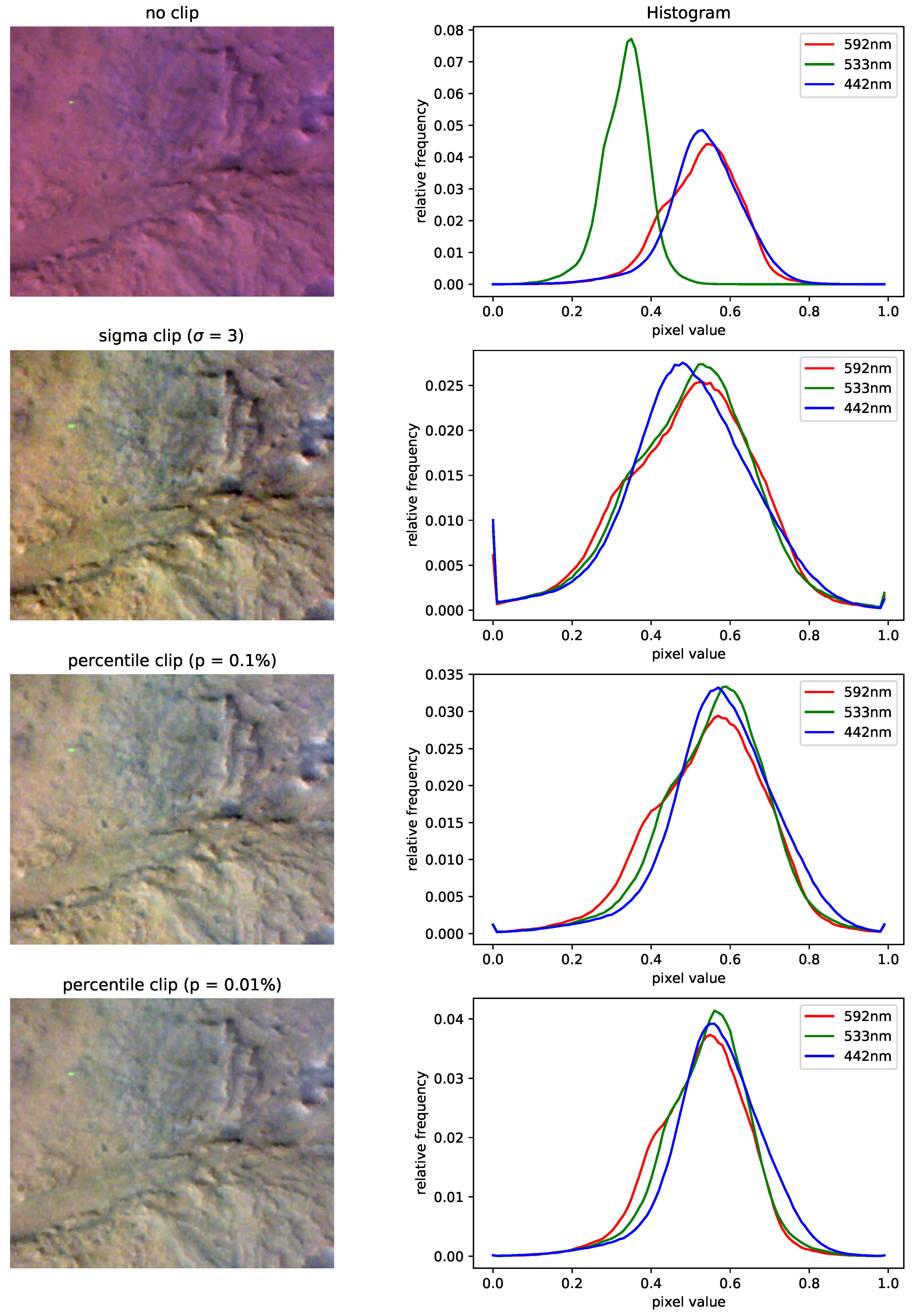
Another preprocessing step is the clipping of CTX and especially of CRISM data. Artifacts such as hot pixels with very high values are present in some CRISM bands of some images. They can distort the normalization of large regions and interfere in training. Figure A2 shows a comparison of different clipping procedures. For this demonstration, no clipping along with three clipping methods are applied channel-wise to the CRISM observation FRT00005C5E, after which each channel is mapped to the interval . A percentile clip of p is taken by setting values below the p-th and above the -th percentile to these boundaries, while 3-sigma clip means the same as described in Section 4.1.1. The left column shows an image section containing a hot pixel in the green channel, whereas the right columns of histograms illustrate the corresponding distribution of pixel values. It can be seen in the top row how, if no clipping is applied, the entire distribution of green values is lowered because of one artifact. A 3-sigma clip, meanwhile, has many pixel values set to boundaries, losing a lot of information. Comparing both percentile clip methods shows how most of all retains the original distribution, while negating the artifacts’ impact, making this the method henceforth used.
Appendix A.2. Data Normalization
While multilayer neural networks with non-linear activation are, in theory, able to learn any mapping between the input and output [49], normalized data have been shown to help with convergence [50]. Two common types of transformations scale values to a predefined range such as 0 to 1 or normalize towards a distribution with a mean of 0 and standard deviation of 1; the latter is used in this work. Problems with non-normalized data occur if features of input or output samples exhibit different orders of magnitude. In classification, for example, larger input features will bias a network’s decision making towards these features. Similarly in regression, the ground-truth features of higher magnitudes will have a disproportionate impact on the loss.
The distribution of reflectance values present in CTX and CRISM cubes exhibits many challenges for machine learning applications. Figure A3 provides an overview of different normalization methods and their impact on the appearance and distribution of values, for one exemplary patch. In order to show biases in color, the patch is displayed by mapping all values to a range, as opposed to channel-wise stretching described in Section 4.1.1.
As seen in the top histogram in Figure A3, one problem is the small magnitude of values, that also lie within a narrow range. Across the entire dataset, all CTX reflectance values lie within the range 0.013 to 0.45, similar to most CRISM bands. Another relevant property of CRISM cubes is the differing magnitudes among spectral bands. All three channels of EVC, for example, exhibit significantly differing reflectance values across the entire dataset, as can be seen when comparing mean reflectance values in Table A1. Not addressing this imbalance before training would bias the network towards neglecting channels with lower values. To remedy this issue, all normalization methods henceforth discussed are implemented on a per-channel basis. This means that transformations are applied to each channel individually, only using the statistical properties of that channel.
Three methods of normalization are discussed and later compared, each representing a trade-off between continuity across neighboring patches and preferred distributions of values within them. On one side of this spectrum lies the normalization of each individual patch during training and testing. This ensures that the distribution of each sample is ideal to maximize the network’s performance. Also, when evaluating new locations on Mars, this method may prove more robust, since the range of values remains near constant. The effects of this can be seen in the second histogram of Figure A3, where each channel is centered around zero and spans over a similar range of values. Therefore, the visualization to the left shows no bias towards any color. Such an approach however removes all continuity between patches, along with any information about absolute radiance in each scene. As a result of that, it is not possible to reverse the normalization to regain original values, when evaluating scenes without ground truth. CTX images evaluated using this approach will inherently show discontinuities between neighboring patches.
Opposite to the first approach is a global normalization. Here statistical properties for the transformation are calculated using data from all available image pairs. Means and standard deviations of each CRISM band and CTX which are used for this normalization are listed in Table A1. The exact same transformation is thus applied to each sample during training and in later deployment. Compared to no normalization, values will be spread apart further and discrepancies between channels are mitigated. This method preserves the ranking of absolute radiance across samples and is easily reversed, allowing the recovery of original values from prediction. Problems with this approach can occur when large datasets with different distributions are considered. Extreme values or biases from certain regions will have an impact on all samples. These properties are seen in the third row of Figure A3, where ranges of values have been expanded and orders of magnitude between bands are closer, although a bias towards red still emerges.
The third proposed method is the normalization of each image pair individually. This represents a compromise between the two previous methods, since a continuous trend across an image remains, while all other image pairs are disregarded. It is again impossible to reverse this transformation in deployment, although a continuity across patches is implicitly trained. As the bottom histogram of Figure A3 shows, distributions are kept closer to each other and occupy a much larger range than with a global transformation, but not as much as a patch-wise normalization.
Figure A2.
Comparison of different clipping methods and their impact on appearance and distribution of pixel values on CRISM observation FRT00005C5E.
Figure A2.
Comparison of different clipping methods and their impact on appearance and distribution of pixel values on CRISM observation FRT00005C5E.

Figure A3.
Impact of different normalization methods on the appearance (left) and distribution of pixel values (right) for one exemplary 256 by 256-pixel EVC CRISM and CTX patch.
Figure A3.
Impact of different normalization methods on the appearance (left) and distribution of pixel values (right) for one exemplary 256 by 256-pixel EVC CRISM and CTX patch.

Appendix B. List of Products
Table A2.
Eberswalde Crater.
| CRISM ID | CTX ID | dt [d] | Overlap [%] | Set |
|---|---|---|---|---|
| FRT00003EEB_07_IF164J_MTR3 | P03_002233_1558_XI_24S033W | 0 | 4.8 | - |
| FRT00008038_07_IF164J_MTR3 | P13_005978_1543_XI_25S032W | 33 | 19.1 | train |
| FRT00009C06_07_IF164J_MTR3 | P01_001534_1559_XI_24S033W | 436 | 5.4 | train |
| FRT0000A30C_07_IF164J_MTR3 | P17_007481_1544_XI_25S033W | 0 | 16.2 | train |
| FRT0000AADE_07_IF164J_MTR3 | P19_008272_1545_XI_25S033W | 0 | 16.7 | train |
| FRT0000B548_07_IF164J_MTR3 | P21_009274_1558_XN_24S033W | 16 | 0.1 | test |
| FRT0000D568_07_IF164J_MTR3 | B03_010764_1560_XI_24S033W | 0 | 16.1 | - |
| FRT00016C5E_07_IF164J_MTR3 | B18_016777_1580_XN_22S034W | 0 | 11.4 | train |
| FRT00019999_07_IF164J_MTR3 | G01_018412_1560_XN_24S033W | 0 | 11.3 | train |
| FRT00019D76_07_IF164J_MTR3 | G01_018623_1555_XN_24S033W | 0 | 1.9 | val |
| FRT0001C383_07_IF164J_MTR3 | G06_020390_1558_XN_24S033W | 0 | 1.9 | train |
Table A3.
Gale Crater.
| CRISM ID | CTX ID | dt [d] | Overlap [%] | Set |
|---|---|---|---|---|
| FRT000037DF_07_IF165J_MTR3 | P02_001897_1747_XI_05S221W | 0 | 0.0 | test |
| FRT000058A3_07_IF165J_MTR3 | P06_003453_1752_XI_04S222W | 0 | 7.8 | train |
| FRT0000901A_07_IF165J_MTR3 | P14_006644_1747_XI_05S222W | 0 | 0.0 | val |
| FRT000095EE_07_IF165J_MTR3 | P15_006855_1746_XN_05S222W | 0 | 0.1 | train |
| FRT0000A091_07_IF165J_MTR3 | P16_007356_1749_XI_05S222W | 0 | 7.8 | train |
| FRT0000A906_07_IF165J_MTR3 | P18_008147_1749_XN_05S222W | 0 | 7.9 | train |
| FRT0000B5A3_07_IF165J_MTR3 | P18_008002_1748_XN_05S222W | 84 | 0.0 | train |
| FRT0000B6F1_07_IF165J_MTR3 | P21_009149_1752_XI_04S222W | 0 | 8.1 | train |
| FRT0000BEE7_07_IF165J_MTR3 | P22_009505_1753_XI_04S222W | 0 | 6.4 | train |
| FRT0000BFCA_07_IF167J_MTR3 | P22_009571_1756_XI_04S222W | 0 | 6.9 | train |
| FRT0000C0EF_07_IF165J_MTR3 | P22_009650_1772_XI_02S222W | 0 | 1.1 | train |
| FRT0000C518_07_IF165J_MTR3 | B01_009861_1753_XI_04S222W | 0 | 2.6 | train |
| FRT0000C620_07_IF166J_MTR3 | B01_009927_1752_XN_04S222W | 0 | 0.2 | - |
Table A4.
Holden Crater.
| CRISM ID | CTX ID | dt [d] | Overlap [%] | Set |
|---|---|---|---|---|
| FRT0000474A_07_IF164J_MTR3 | P04_002721_1538_XI_26S034W | 0 | 0.0 | test |
| FRT00004F2F_07_IF164J_MTR3 | P04_002721_1538_XI_26S034W | 28 | 9.6 | train |
| FRT00006246_07_IF164J_MTR3 | P04_002721_1538_XI_26S034W | 105 | 9.6 | train |
| FRT00009172_07_IF164J_MTR3 | P14_006690_1512_XI_28S034W | 0 | 0.0 | train |
| FRT0000955B_07_IF164J_MTR3 | P15_006835_1536_XN_26S035W | 0 | 6.9 | - |
| FRT00009D17_07_IF164J_MTR3 | P16_007191_1536_XI_26S035W | 0 | 4.0 | train |
| FRT0000A98D_07_IF164J_MTR3 | P18_008193_1536_XN_26S034W | 0 | 3.2 | train |
| FRT0000ABB5_07_IF164J_MTR3 | P19_008338_1531_XN_26S035W | 0 | 0.0 | val |
| FRT0000B678_07_IF164J_MTR3 | P22_009696_1531_XI_26S034W | 44 | 0.9 | train |
| FRT0000BB9F_07_IF164J_MTR3 | B02_010540_1532_XI_26S034W | 94 | 0.6 | train |
| FRT0000C1D1_07_IF164J_MTR3 | P22_009696_1531_XI_26S034W | 0 | 0.0 | train |
Table A5.
Jezero Crater.
| CRISM ID | CTX ID | dt [d] | Overlap [%] | Set |
|---|---|---|---|---|
| FRT000047A3_07_IF166J_MTR3 | P04_002743_1987_XI_18N282W | 0 | 11.6 | train |
| FRT00005850_07_IF167J_MTR3 | P06_003442_1987_XI_18N282W | 0 | 1.6 | train |
| FRT00005C5E_07_IF166J_MTR3 | P06_003442_1987_XI_18N282W | 28 | 8.4 | train |
| FRT000066A4_07_IF166J_MTR3 | P04_002743_1987_XI_18N282W | 121 | 18.1 | train |
| FRT0001182A_07_IF165J_MTR3 | B18_016786_1978_XN_17N283W | 352 | 0.0 | test |
| FRT0001642E_07_IF166J_MTR3 | B18_016509_1978_XN_17N282W | 0 | 1.4 | val |
| FRT00017103_07_IF165J_MTR3 | B19_016931_1975_XN_17N283W | 0 | 1.4 | train |
| FRT0001ECBA_07_IF166J_MTR3 | G13_023102_1986_XN_18N282W | 0 | 7.9 | train |
| FRT0001FB74_07_IF166J_MTR3 | G14_023669_1985_XN_18N282W | 0 | 15.0 | train |
| FRT00021DA6_07_IF166J_MTR3 | G14_023669_1985_XN_18N282W | 121 | 17.5 | train |
Table A6.
Mawrth Vallis.
| CRISM ID | CTX ID | dt [d] | Overlap [%] | Set |
|---|---|---|---|---|
| FRT000089F7_07_IF166J_MTR3 | P13_005964_2046_XI_24N019W | 0 | 18.7 | train |
| FRT000094F6_07_IF166J_MTR3 | P15_006821_2045_XN_24N019W | 0 | 3.3 | train |
| FRT0000A600_07_IF167J_MTR3 | P17_007612_2043_XI_24N018W | 0 | 12.3 | train |
| FRT0000B141_07_IF167J_MTR3 | P20_008825_2042_XI_24N019W | 0 | 12.0 | train |
| FRT0000B643_07_IF166J_MTR3 | P20_008825_2042_XI_24N019W | 23 | 3.2 | train |
| FRT0000BB59_07_IF166J_MTR3 | B03_010816_2041_XI_24N019W | 116 | 1.9 | train |
| FRT00016E2D_07_IF166J_MTR3 | B18_016829_2037_XI_23N018W | 0 | 0.0 | test |
| FRT00019AA0_07_IF166J_MTR3 | G01_018464_2046_XN_24N018W | 0 | 0.0 | val |
| FRT0001EB5F_07_IF166J_MTR3 | G12_023000_2042_XN_24N019W | 0 | 18.8 | train |
| FRT0001EC38_07_IF166J_MTR3 | G11_022499_2041_XN_24N019W | 44 | 0.6 | train |
| FRT00020B2B_07_IF166J_MTR3 | G17_024688_2041_XN_24N019W | 22 | 14.8 | train |
| FRT00021BCB_07_IF166J_MTR3 | G18_025123_2054_XN_25N019W | 0 | 3.3 | train |
Table A7.
Melas Chasma.
| CRISM ID | CTX ID | dt [d] | Overlap [%] | Set |
|---|---|---|---|---|
| FRT000043C6_07_IF164J_MTR3 | P04_002551_1712_XI_08S076W | 0 | 2.4 | train |
| FRT00006347_07_IF164J_MTR3 | P08_004107_1679_XI_12S076W | 0 | 3.7 | train |
| FRT0000827D_07_IF164J_MTR3 | P08_004252_1714_XI_08S077W | 110 | 0.0 | test |
| FRT00009B66_07_IF164J_MTR3 | P17_007667_1702_XI_09S076W | 45 | 5.2 | train |
| FRT0000A244_07_IF164J_MTR3 | P16_007443_1714_XN_08S077W | 0 | 0.0 | val |
| FRT0000AA51_07_IF164J_MTR3 | P22_009592_1704_XI_09S077W | 106 | 0.0 | train |
| FRT0000AC5C_07_IF164J_MTR3 | P19_008379_1701_XI_09S076W | 0 | 1.9 | train |
| FRT0000AD3D_07_IF164J_MTR3 | P20_008669_1703_XI_09S076W | 0 | 0.0 | train |
| FRT0000B77E_07_IF164J_MTR3 | P22_009803_1699_XN_10S077W | 49 | 0.0 | train |
| FRT0000C00F_07_IF164J_MTR3 | P22_009592_1704_XI_09S077W | 0 | 0.0 | train |
| FRT0000C67C_07_IF164J_MTR3 | B01_009948_1704_XI_09S077W | 0 | 0.0 | - |
| FRT0000CB1A_07_IF164J_MTR3 | B01_010159_1697_XI_10S077W | 0 | 0.0 | train |
| FRT00010122_07_IF164J_MTR3 | B04_011293_1708_XI_09S077W | 0 | 0.0 | train |
| FRT0001070E_07_IF166J_MTR3 | B05_011504_1700_XN_10S075W | 0 | 0.0 | train |
| FRT000109B6_07_IF164J_MTR3 | B05_011649_1701_XN_09S076W | 0 | 3.0 | train |
References
- Zurek, R.W.; Smrekar, S.E. An overview of the Mars Reconnaissance Orbiter (MRO) science mission. J. Geophys. Res. Planets 2007, 112. [Google Scholar] [CrossRef] [Green Version]
- Murchie, S.; Arvidson, R.; Bedini, P.; Beisser, K.; Bibring, J.P.; Bishop, J.; Boldt, J.; Cavender, P.; Choo, T.; Clancy, R.; et al. Compact reconnaissance imaging spectrometer for Mars (CRISM) on Mars reconnaissance orbiter (MRO). J. Geophys. Res. Planets 2007, 112. [Google Scholar] [CrossRef]
- Malin, M.C.; Bell, J.F.; Cantor, B.A.; Caplinger, M.A.; Calvin, W.M.; Clancy, R.T.; Edgett, K.S.; Edwards, L.; Haberle, R.M.; James, P.B.; et al. Context camera investigation on board the Mars Reconnaissance Orbiter. J. Geophys. Res. Planets 2007, 112. [Google Scholar] [CrossRef] [Green Version]
- Pelkey, S.; Mustard, J.; Murchie, S.; Clancy, R.; Wolff, M.; Smith, M.; Milliken, R.; Bibring, J.P.; Gendrin, A.; Poulet, F.; et al. CRISM multispectral summary products: Parameterizing mineral diversity on Mars from reflectance. J. Geophys. Res. Planets 2007, 112. [Google Scholar] [CrossRef]
- Koßmann, D.; Wilhelm, T.; Fink, G.A. Towards tackling multi-label imbalances in remote sensing imagery. In Proceedings of the 2020 25th International Conference on Pattern Recognition (ICPR), Milan, Italy, 10–15 January 2021; pp. 5782–5789. [Google Scholar]
- Gewali, U.B.; Monteiro, S.T.; Saber, E. Machine learning based hyperspectral image analysis: A survey. arXiv 2018, arXiv:1802.08701. [Google Scholar]
- Qian, Y.; Xiao, L.; Head, J.W.; Wöhler, C.; Bugiolacchi, R.; Wilhelm, T.; Althoff, S.; Ye, B.; He, Q.; Yuan, Y.; et al. Copernican-Aged (< 200 Ma) Impact Ejecta at the Chang’e-5 Landing Site: Statistical Evidence From Crater Morphology, Morphometry, and Degradation Models. Geophys. Res. Lett. 2021, 48, e2021GL095341. [Google Scholar]
- Wilhelm, T.; Wöhler, C. Uncertainty Guided Recognition of Tiny Craters on the Moon. In Proceedings of the 2020 25th International Conference on Pattern Recognition (ICPR), Milan, Italy, 10–15 January 2021; pp. 5198–5205. [Google Scholar]
- Wilhelm, T.; Geis, M.; Püttschneider, J.; Sievernich, T.; Weber, T.; Wohlfarth, K.; Wöhler, C. Domars16k: A diverse dataset for weakly supervised geomorphologic analysis on mars. Remote Sens. 2020, 12, 3981. [Google Scholar] [CrossRef]
- Dundar, M.; Ehlmann, B.L.; Leask, E.K. Machine-Learning-Driven New Geologic Discoveries at Mars Rover Landing Sites: Jezero and NE Syrtis. arXiv 2019, arXiv:1909.02387. [Google Scholar]
- Isola, P.; Zhu, J.Y.; Zhou, T.; Efros, A.A. Image-to-image translation with conditional adversarial networks. In Proceedings of the IEEE Conference on Computer Vision and Pattern Recognition, Honolulu, HI, USA, 21–26 July 2017; pp. 1125–1134. [Google Scholar]
- Pang, Y.; Lin, J.; Qin, T.; Chen, Z. Image-to-Image Translation: Methods and Applications. arXiv 2021, arXiv:2101.08629. [Google Scholar] [CrossRef]
- Fuentes Reyes, M.; Auer, S.; Merkle, N.; Henry, C.; Schmitt, M. Sar-to-optical image translation based on conditional generative adversarial networks—Optimization, opportunities and limits. Remote Sens. 2019, 11, 2067. [Google Scholar] [CrossRef] [Green Version]
- Robertson, A.R. The CIE 1976 color-difference formulae. Color Res. Appl. 1977, 2, 7–11. [Google Scholar] [CrossRef]
- Jain, A.K. Fundamentals of Digital Image Processing; Prentice-Hall, Inc.: Upper Saddle River, NJ, USA, 1989. [Google Scholar]
- Charpiat, G.; Hofmann, M.; Schölkopf, B. Automatic image colorization via multimodal predictions. In Proceedings of the European Conference on Computer Vision, Marseille, France, 12–18 October 2008; Springer: Berlin/Heidelberg, Germany, 2008; pp. 126–139. [Google Scholar]
- Zhang, R.; Isola, P.; Efros, A.A. Colorful image colorization. In Proceedings of the European Conference on Computer Vision, Amsterdam, The Netherlands, 11–14 October 2016; Springer: Berlin/Heidelberg, Germany, 2016; pp. 649–666. [Google Scholar]
- Nazeri, K.; Ng, E.; Ebrahimi, M. Image colorization using generative adversarial networks. In Proceedings of the International Conference on Articulated Motion and Deformable Objects, Palma de Mallorca, Spain, 12–13 July 2018; Springer: Berlin/Heidelberg, Germany, 2018; pp. 85–94. [Google Scholar]
- Bhoi, A. Monocular depth estimation: A survey. arXiv 2019, arXiv:1901.09402. [Google Scholar]
- Jiao, J.; Cao, Y.; Song, Y.; Lau, R. Look deeper into depth: Monocular depth estimation with semantic booster and attention-driven loss. In Proceedings of the European Conference on Computer Vision (ECCV), Munich, Germany, 8–14 September 2018; pp. 53–69. [Google Scholar]
- Fu, H.; Gong, M.; Wang, C.; Batmanghelich, K.; Tao, D. Deep ordinal regression network for monocular depth estimation. In Proceedings of the IEEE Conference on Computer Vision and Pattern Recognition, Salt Lake City, UT, USA, 18–22 June 2018; pp. 2002–2011. [Google Scholar]
- Winship, C.; Mare, R.D. Regression models with ordinal variables. Am. Sociol. Rev. 1984, 49, 512–525. [Google Scholar] [CrossRef]
- Minaee, S.; Boykov, Y.Y.; Porikli, F.; Plaza, A.J.; Kehtarnavaz, N.; Terzopoulos, D. Image segmentation using deep learning: A survey. IEEE Trans. Pattern Anal. Mach. Intell. 2021, 44, 3523–3542. [Google Scholar] [CrossRef]
- Simonyan, K.; Zisserman, A. Very deep convolutional networks for large-scale image recognition. arXiv 2014, arXiv:1409.1556. [Google Scholar]
- He, K.; Zhang, X.; Ren, S.; Sun, J. Deep residual learning for image recognition. In Proceedings of the IEEE Conference on Computer Vision and Pattern Recognition, Las Vegas, NV, USA, 27–30 June 2016; pp. 770–778. [Google Scholar]
- Huang, G.; Liu, Z.; Van Der Maaten, L.; Weinberger, K.Q. Densely connected convolutional networks. In Proceedings of the IEEE Conference on Computer Vision and Pattern Recognition, Honolulu, HI, USA, 21–26 July 2017; pp. 4700–4708. [Google Scholar]
- Tan, M.; Le, Q. Efficientnet: Rethinking model scaling for convolutional neural networks. In Proceedings of the International Conference on Machine Learning. PMLR, Long Beach, CA, USA, 9–15 June 2019; pp. 6105–6114. [Google Scholar]
- Xu, J.; Pan, Y.; Pan, X.; Hoi, S.; Yi, Z.; Xu, Z. RegNet: Self-Regulated Network for Image Classification. arXiv 2021, arXiv:2101.00590. [Google Scholar] [CrossRef]
- Chaurasia, A.; Culurciello, E. Linknet: Exploiting encoder representations for efficient semantic segmentation. In Proceedings of the 2017 IEEE Visual Communications and Image Processing (VCIP), St. Petersburg, FL, USA, 10–13 December 2017; pp. 1–4. [Google Scholar]
- Kirillov, A.; He, K.; Girshick, R.; Dollár, P. A Unified Architecture for Instance and Semantic Segmentation. 2017. Available online: http://presentations.cocodataset.org/COCO17-Stuff-FAIR.pdf (accessed on 14 June 2022).
- Fan, T.; Wang, G.; Li, Y.; Wang, H. Ma-net: A multi-scale attention network for liver and tumor segmentation. IEEE Access 2020, 8, 179656–179665. [Google Scholar] [CrossRef]
- Zhou, Z.; Siddiquee, M.M.R.; Tajbakhsh, N.; Liang, J. Unet++: A nested u-net architecture for medical image segmentation. In Deep Learning in Medical Image Analysis and Multimodal Learning for Clinical Decision Support; Springer: Berlin/Heidelberg, Germany, 2018; pp. 3–11. [Google Scholar]
- Zhao, H.; Shi, J.; Qi, X.; Wang, X.; Jia, J. Pyramid scene parsing network. In Proceedings of the IEEE Conference on Computer Vision and Pattern Recognition, Honolulu, HI, USA, 21–26 July 2017; pp. 2881–2890. [Google Scholar]
- Ronneberger, O.; Fischer, P.; Brox, T. U-net: Convolutional networks for biomedical image segmentation. In Proceedings of the International Conference on Medical image computing and computer-assisted intervention, Munich, Germany, 5–9 October 2015; Springer: Berlin/Heidelberg, Germany, 2015; pp. 234–241. [Google Scholar]
- Li, B.; Dai, Y.; He, M. Monocular depth estimation with hierarchical fusion of dilated cnns and soft-weighted-sum inference. Pattern Recognit. 2018, 83, 328–339. [Google Scholar] [CrossRef] [Green Version]
- Dickson, J.L.; Kerber, L.A.; Fassett, C.I.; Ehlmann, B.L. A Global, Blended CTX Mosaic of Mars with Vectorized Seam Mapping: A New Mosaicking Pipeline Using Principles of Non-Destructive Image Editing. In Proceedings of the 49th Lunar and Planetary Science Conference, The Woodlands, TX, USA, 19–23 March 2018; Lunar and Planetary Institute: Houston, TX, USA, 2018; p. Abstract #2480. [Google Scholar]
- Mouginis-Mark, P.J.; Garbeil, H. CTX Digital Elevation Models Facilitate Geomorphic Analysis of Mars. In Proceedings of the 50th Lunar and Planetary Science Conference, The Woodlands, TX, USA, 18–22 March 2019; Lunar and Planetary Institute: Houston, TX, USA, 2019; p. Abstract #1069. [Google Scholar]
- Boain, R.J. AB-Cs of Sun-Synchronous Orbit Mission Design. In Proceedings of the 2004 In 14th AAS/AIAA Space Flight Mechanics Meeting, Maui, HI, USA, 8–12 February 2004. [Google Scholar]
- Munappy, A.; Bosch, J.; Olsson, H.H.; Arpteg, A.; Brinne, B. Data management challenges for deep learning. In Proceedings of the 2019 45th Euromicro Conference on Software Engineering and Advanced Applications (SEAA), Kallithea-Chalkidiki, Greece, 28–30 August 2019; pp. 140–147. [Google Scholar]
- Bennett, K.J.; Wang, J.; Scholes, D. Accessing PDS Data in Pipeline Processing and Websites Through PDS Geosciences Orbital Data Explorer’s Web-Based API (REST) Interface. In Proceedings of the 45th Lunar and Planetary Science Conference, The Woodlands, TX, USA, 17–21 March 2021; Lunar and Planetary Institute: Houston, TX, USA, 2014; p. Abstract #1026. [Google Scholar]
- Deng, J.; Dong, W.; Socher, R.; Li, L.J.; Li, K.; Fei-Fei, L. Imagenet: A large-scale hierarchical image database. In Proceedings of the 2009 IEEE Conference on Computer Vision and Pattern Recognition, Miami, FL, USA, 20–25 June 2009; pp. 248–255. [Google Scholar]
- Buda, M.; Saha, A.; Mazurowski, M.A. Association of genomic subtypes of lower-grade gliomas with shape features automatically extracted by a deep learning algorithm. Comput. Biol. Med. 2019, 109, 218–225. [Google Scholar] [CrossRef] [Green Version]
- Lin, M.; Chen, H.; Sun, X.; Qian, Q.; Li, H.; Jin, R. Neural architecture design for gpu-efficient networks. arXiv 2020, arXiv:2006.14090. [Google Scholar]
- Fergason, R.; Hare, T.; Laura, J. HRSC and MOLA Blended Digital Elevation Model at 200 m v2, Astrogeology PDS Annex; US Geological Survey: Flagstaff, AZ, USA, 2018. [Google Scholar]
- Viviano-Beck, C.E.; Seelos, F.P.; Murchie, S.L.; Kahn, E.G.; Seelos, K.D.; Taylor, H.W.; Taylor, K.; Ehlmann, B.L.; Wiseman, S.M.; Mustard, J.F.; et al. Revised CRISM spectral parameters and summary products based on the currently detected mineral diversity on Mars. J. Geophys. Res. Planets 2014, 119, 1403–1431. [Google Scholar] [CrossRef] [Green Version]
- Sucharski, T.; Mapel, J.; jcwbacker; Kristin; Lee, K.; AgoinsUSGS; Shepherd, M.; Ryan Combs, C., Jr.; dcookastro; Stapleton, S.; et al. USGS-Astrogeology/ISIS3: ISIS4.1.0 Public Release. 2020. Available online: https://zenodo.org/record/3780717/export/hx#.YtYHU3ZByUk (accessed on 14 June 2022).
- Wang, Y.; Wu, B. Investigation of boresight offsets and co-registration of HiRISE and CTX imagery for precision Mars topographic mapping. Planet. Space Sci. 2017, 139, 18–30. [Google Scholar] [CrossRef]
- Scheffler, D.; Hollstein, A.; Diedrich, H.; Segl, K.; Hostert, P. AROSICS: An Automated and Robust Open-Source Image Co-Registration Software for Multi-Sensor Satellite Data. Remote Sens. 2017, 9, 676. [Google Scholar] [CrossRef] [Green Version]
- Hornik, K.; Stinchcombe, M.; White, H. Multilayer feedforward networks are universal approximators. Neural Netw. 1989, 2, 359–366. [Google Scholar] [CrossRef]
- Ioffe, S.; Szegedy, C. Batch normalization: Accelerating deep network training by reducing internal covariate shift. In Proceedings of the International Conference on Machine Learning, Lille, France, 6–11 July 2015; pp. 448–456. [Google Scholar]
Figure 1.
Illustration of a typical U-Net-style [34] neural network architecture used in this work. Each neural network used in this work has a related structure. The network consists of two parts: an encoder (orange) and a decoder (green). The flow of the signal through the network is indicated by arrows. At the end, the neural network predicts pixel-wise bands (e.g., red, green, and blue) from the monochromatic input image (gray).

Figure 2.
Two number lines with markers for bin edges and their representative values visualizing the difference between equidistant binning (top) and spacing-increasing discretization (bottom).
Figure 2.
Two number lines with markers for bin edges and their representative values visualizing the difference between equidistant binning (top) and spacing-increasing discretization (bottom).

Figure 3.
Enhanced visible color image of CRISM observation FRT0000C518 (left) and corresponding cut-out of CTX B01_009861_1753 (right).
Figure 3.
Enhanced visible color image of CRISM observation FRT0000C518 (left) and corresponding cut-out of CTX B01_009861_1753 (right).

Figure 4.
CRISM reflectance spectrum (right) next to a mafic (center) and enhanced visible color (left) CRISM FRT000066A4 browse product.
Figure 4.
CRISM reflectance spectrum (right) next to a mafic (center) and enhanced visible color (left) CRISM FRT000066A4 browse product.

Figure 5.
Jezero crater with multiple CRISM observations overlaid on CTX mosaic.

Figure 6.
Example of CRISM observation deemed too noisy for training (right) next to corresponding CTX cut-out (left).
Figure 6.
Example of CRISM observation deemed too noisy for training (right) next to corresponding CTX cut-out (left).

Figure 7.
Appearance comparison of six EVC test patches across different model architectures.

Figure 8.
Channel-wise histogram comparison of six EVC test patches across different model architectures. Rows correspond to the respective rows in Figure 7.
Figure 8.
Channel-wise histogram comparison of six EVC test patches across different model architectures. Rows correspond to the respective rows in Figure 7.
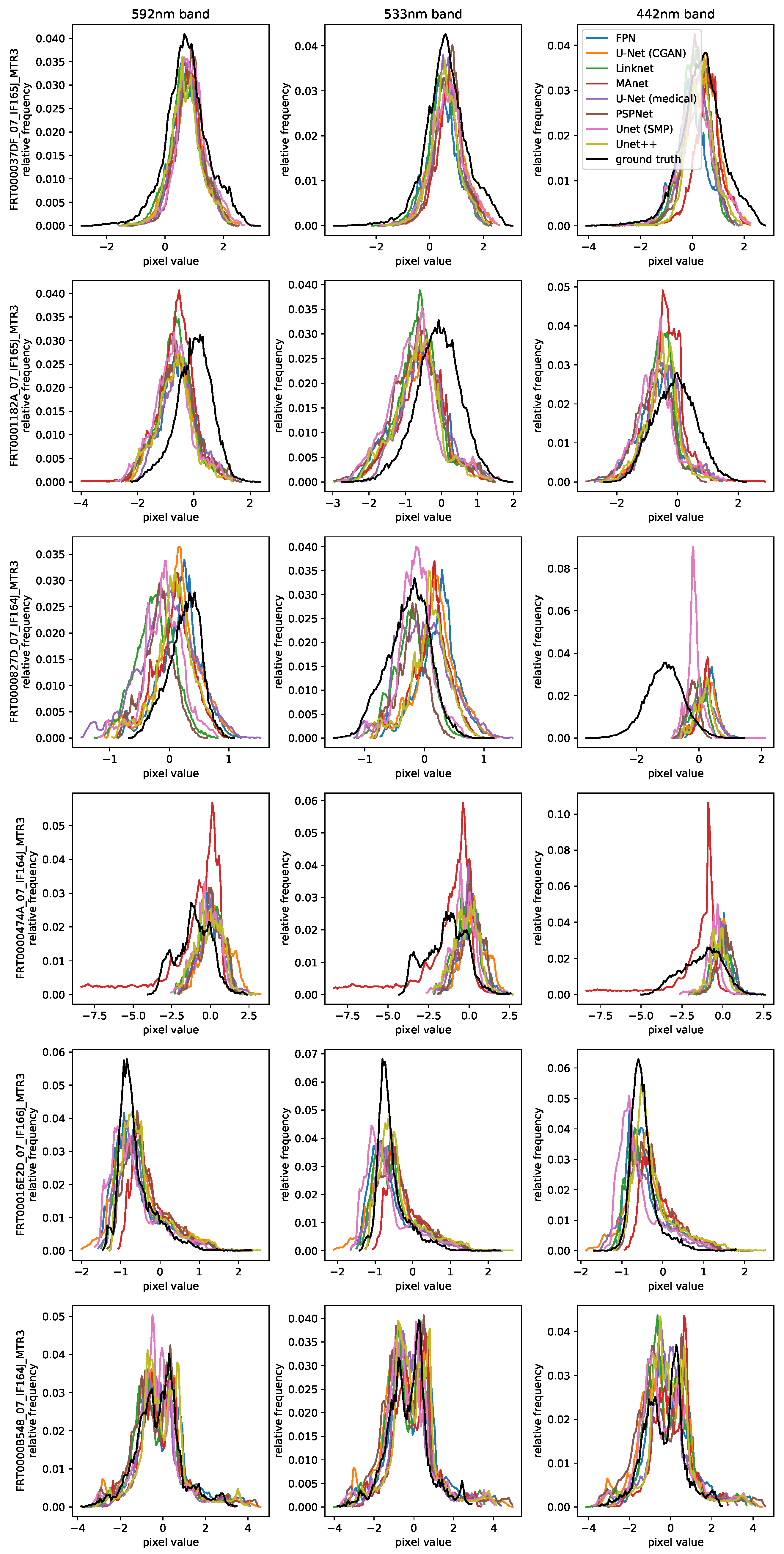
Figure 9.
Appearance comparison of six EVC test patches across different encoder networks.

Figure 10.
Examples of artifacts within the EVC output of three encoders that occasionally occur.

Figure 11.
Full CTX-CRISM EVC image pair (top row) and model predictions with different strides and averaging techniques (middle and bottom row).
Figure 11.
Full CTX-CRISM EVC image pair (top row) and model predictions with different strides and averaging techniques (middle and bottom row).

Figure 12.
Appearance comparison of six EVC test patches across different normalization methods.

Figure 13.
Full CTX-CRISM EVC image pair (top row) and model predictions with different normalization methods (middle and bottom row).
Figure 13.
Full CTX-CRISM EVC image pair (top row) and model predictions with different normalization methods (middle and bottom row).

Figure 14.
Mawrth Vallis’ CTX (left), DEM (center) and EVC CRISM (right) images from the validation set on top, and model predictions with (right) and without DEM (left) as input on the bottom.
Figure 14.
Mawrth Vallis’ CTX (left), DEM (center) and EVC CRISM (right) images from the validation set on top, and model predictions with (right) and without DEM (left) as input on the bottom.

Figure 15.
Appearance comparison of six EVC test patches across different bin counts, reconstructed using the weighted sum method.
Figure 15.
Appearance comparison of six EVC test patches across different bin counts, reconstructed using the weighted sum method.

Figure 16.
Two marked pixels from a predicted EVC patch (left) and their associated bin probabilities across three bands from a faulty region (center) and a regular region (right).
Figure 16.
Two marked pixels from a predicted EVC patch (left) and their associated bin probabilities across three bands from a faulty region (center) and a regular region (right).

Figure 17.
Appearance comparison of six EVC test patches across different modifications to the classification approach.
Figure 17.
Appearance comparison of six EVC test patches across different modifications to the classification approach.

Figure 18.
Full Jezero crater validation CTX-CRISM EVC pair (top row), with prediction using the baseline classification model (bottom left) trained with an L1-loss component (bottom right).
Figure 18.
Full Jezero crater validation CTX-CRISM EVC pair (top row), with prediction using the baseline classification model (bottom left) trained with an L1-loss component (bottom right).

Figure 19.
Appearance comparison of six test patches in the visual spectrum (EVC) and infrared (FC), predicted by two separate models.
Figure 19.
Appearance comparison of six test patches in the visual spectrum (EVC) and infrared (FC), predicted by two separate models.

Figure 20.
Full EVC image predictions of the proposed approach. From top to bottom: Jezero crater training CTX-CRISM pair, Gale crater training CTX-CRISM pair, Mawrth Vallis training CTX-CRISM pair, Jezero crater validation CTX-CRISM pair, and Melas Chasma CTX-CRISM pair excluded from training with stripe artifacts spanning the entire CRISM image.

Figure 21.
Full EVC image predictions of the proposed approach from the test set. From top to bottom: Gale crater test CTX-CRISM pair and Mawrth Vallis test CTX-CRISM pair.
Figure 21.
Full EVC image predictions of the proposed approach from the test set. From top to bottom: Gale crater test CTX-CRISM pair and Mawrth Vallis test CTX-CRISM pair.

Figure 22.
CTX observation B03_010816_2041_XI_24N019W (left) next to predicted EVC browse product with s = 2 and Gauss averaging (right).
Figure 22.
CTX observation B03_010816_2041_XI_24N019W (left) next to predicted EVC browse product with s = 2 and Gauss averaging (right).

Table 1.
Location names, bounding boxes and number of MTRDR found within that form the dataset.
| Latitude (°) | Longitude (°) | ||||
|---|---|---|---|---|---|
| Location | Min | Max | Western | Eastern | Number of MTRDR |
| Eberswalde crater | −24.5 | −23.4 | −34 | −32.7 | 11 |
| Mawrth Vallis | 23.3 | 24.6 | −19.6 | −18.4 | 12 |
| Holden crater | −27.6 | −25.9 | −36 | −34 | 11 |
| Melas Chasma | −10.5 | −8.7 | −78 | −75 | 15 |
| Jezero crater | 18 | 18.8 | 77.2 | 78.4 | 10 |
| Gale crater | −0.9 | −3.8 | 135.9 | 139.9 | 13 |
Table 2.
Comparison of performance metrics across different model architectures. Root mean squared error (RMSE), cosine similarity (Cosine), and the Pearson correlation coefficient (PCC) are presented. Memory reflects the maximum memory consumption during training and time reflects the average training time per epoch.
| Model Architecture | RMSE | Cosine | PCC | Train Loss | # Parameters | Memory (MB) | Time (s) |
|---|---|---|---|---|---|---|---|
| FPN [30] | 0.657 | 0.556 | 0.618 | 0.141 | 13,041,219 | 2236 | 24.31 |
| Linknet [29] | 0.650 | 0.567 | 0.604 | 0.163 | 11,657,571 | 2668 | 27.32 |
| MAnet [31] | 0.890 | 0.547 | 0.612 | 0.286 | 21,669,491 | 3014 | 37.47 |
| PSPNet [33] | 0.673 | 0.530 | 0.602 | 0.213 | 11,332,771 | 1696 | 14.12 |
| U-Net (CGAN) [18] | 0.688 | 0.545 | 0.612 | 0.265 | 54,411,907 | 5978 | 61.61 |
| U-Net (medical) [42] | 0.673 | 0.532 | 0.556 | 0.213 | 7,762,531 | 5692 | 61.73 |
| Unet (SMP) [34] | 0.666 | 0.546 | 0.586 | 0.153 | 14,322,227 | 3442 | 31.72 |
| Unet++ [32] | 0.668 | 0.553 | 0.601 | 0.153 | 15,964,467 | 5448 | 64.79 |
Table 3.
Comparison of EVC performance metrics across different encoder networks. Root mean squared error (RMSE), cosine similarity (Cosine), and the Pearson correlation coefficient (PCC) are presented. Memory reflects the maximum memory consumption during training and time reflects the average training time per epoch.
| Encoder | RMSE | Cosine | PCC | Train Loss | # Parameters | Memory (MB) | Time (s) |
|---|---|---|---|---|---|---|---|
| DenseNet121 [26] | 0.681 | 0.533 | 0.602 | 0.218 | 13,601,651 | 7340 | 81.38 |
| EfficientNet [27] | 0.680 | 0.543 | 0.598 | 0.174 | 6,251,183 | 4664 | 59.46 |
| GerNet_s [43] | 0.674 | 0.545 | 0.586 | 0.219 | 12,827,394 | 3436 | 42.37 |
| RegNetX_002 [28] | 0.666 | 0.557 | 0.610 | 0.204 | 4,780,611 | 3444 | 46.01 |
| RegNetY_002 [28] | 0.677 | 0.538 | 0.604 | 0.208 | 5,258,815 | 3388 | 49.91 |
| ResNet18 [25] | 0.679 | 0.535 | 0.601 | 0.225 | 14,322,227 | 3636 | 39.83 |
| VGG11 [24] | 0.658 | 0.556 | 0.586 | 0.108 | 18,253,171 | 4630 | 57.49 |
Table 4.
Differences in metrics when evaluating full EVC images. CTX image P21_009274_1558_XN_24S033W and CRISM image FRT0000B548_07_IF164J_MTR3 were used. Root mean squared error (RMSE), cosine similarity (Cosine), and the Pearson correlation coefficient (PCC) are presented. s indicates the used stride and the checkmark indicated in the Gaussian weighting column indicates if weighted averages were computed.
| s | Gaussian Weighting | RMSE | Cosine | PCC |
|---|---|---|---|---|
| 1 | 0.528 | 0.777 | 0.809 | |
| 2 | 0.493 | 0.802 | 0.834 | |
| 3 | 0.485 | 0.809 | 0.843 | |
| 2 | ✔ | 0.494 | 0.801 | 0.833 |
Table 5.
Ablation study of different models, with EVC predictions channel-wise scaled to a [0, 1] range for better comparability. Root mean squared error (RMSE), cosine similarity (Cosine), and the Pearson correlation coefficient (PCC) are presented. The checkmark indicates if a certain feature is activated.
| Normalization | Regression | with DEM | Classification | with L1-Loss | RMSE | Cosine | PCC |
|---|---|---|---|---|---|---|---|
| none | ✔ | 0.157 | 0.950 | 0.445 | |||
| global | ✔ | 0.161 | 0.950 | 0.510 | |||
| image-wise | ✔ | 0.133 | 0.962 | 0.618 | |||
| patch-wise | ✔ | 0.137 | 0.959 | 0.591 | |||
| image-wise | ✔ | 0.124 | 0.969 | 0.640 | |||
| image-wise | ✔ | ✔ | 0.121 | 0.967 | 0.643 | ||
| image-wise | ✔ | 0.120 | 0.968 | 0.650 | |||
| image-wise | ✔ | ✔ | 0.119 | 0.967 | 0.636 |
Table 6.
Comparison of EVC performance metrics across different bin counts.
| RMSE | Coss | pcc | Train Loss | # Parameters | Memory (MB) | Time (s) | |
|---|---|---|---|---|---|---|---|
| 10 | 0.644 | 0.589 | 0.627 | 0.562 | 6,254,663 | 6992 | 60.19 |
| 20 | 0.640 | 0.585 | 0.637 | 1.061 | 6,259,013 | 7712 | 59.35 |
| 40 | 0.629 | 0.607 | 0.628 | 1.703 | 6,267,713 | 9396 | 61.57 |
| 80 | 0.635 | 0.588 | 0.630 | 2.449 | 6,285,113 | 11,588 | 73.55 |
Table 7.
Ablation study of evaluated full EVC images. All images were computed with a stride of 2 and Gaussian weighting.
Table 7.
Ablation study of evaluated full EVC images. All images were computed with a stride of 2 and Gaussian weighting.
| CTX ID | CRISM ID | RMSE | COSS | PCC | Set |
|---|---|---|---|---|---|
| B19_016931_1975_XN_17N283W | FRT00017103_07_IF165J_MTR3 | 0.441 | 0.844 | 0.845 | train |
| B01_009861_1753_XI_04S222W | FRT0000C518_07_IF165J_MTR3 | 0.224 | 0.959 | 0.960 | train |
| P17_007612_2043_XI_24N018W | FRT0000A600_07_IF167J_MTR3 | 0.300 | 0.926 | 0.928 | train |
| B18_016509_1978_XN_17N282W | FRT0001642E_07_IF166J_MTR3 | 0.558 | 0.731 | 0.735 | val |
| P02_001897_1747_XI_05S221W | FRT000037DF_07_IF165J_MTR3 | 0.552 | 0.738 | 0.815 | test |
| B18_016829_2037_XI_23N018W | FRT00016E2D_07_IF166J_MTR3 | 0.432 | 0.838 | 0.846 | test |
| B01_009948_1704_XI_09S077W | FRT0000C67C_07_IF164J_MTR3 | 0.521 | 0.796 | 0.815 | - |
Publisher’s Note: MDPI stays neutral with regard to jurisdictional claims in published maps and institutional affiliations. |
© 2022 by the authors. Licensee MDPI, Basel, Switzerland. This article is an open access article distributed under the terms and conditions of the Creative Commons Attribution (CC BY) license (https://creativecommons.org/licenses/by/4.0/).
Share and Cite
MDPI and ACS Style
Stepcenkov, S.; Wilhelm, T.; Wöhler, C. Learning the Link between Albedo and Reflectance: Machine Learning-Based Prediction of Hyperspectral Bands from CTX Images. Remote Sens. 2022, 14, 3457. https://doi.org/10.3390/rs14143457
AMA Style
Stepcenkov S, Wilhelm T, Wöhler C. Learning the Link between Albedo and Reflectance: Machine Learning-Based Prediction of Hyperspectral Bands from CTX Images. Remote Sensing. 2022; 14(14):3457. https://doi.org/10.3390/rs14143457
Chicago/Turabian StyleStepcenkov, Sergej, Thorsten Wilhelm, and Christian Wöhler. 2022. "Learning the Link between Albedo and Reflectance: Machine Learning-Based Prediction of Hyperspectral Bands from CTX Images" Remote Sensing 14, no. 14: 3457. https://doi.org/10.3390/rs14143457
Note that from the first issue of 2016, this journal uses article numbers instead of page numbers. See further details here.