
Improved ENSO and PDO Prediction Skill Resulting from Finer Parameterization Schemes in a CGCM
by
 ,
,
Yuxing Yang
1, 
Xiaokai Hu
2,
Guanghong Liao
2,*,
Qian Cao
3,
Sijie Chen
3,
Hui Gao
3 and
Xiaowei Wei
3 1
Key Laboratory of Ocean Circulation and Waves, Institute of Oceanology, Chinese Academy of Sciences, Center for Ocean Mega-Science, Chinese Academy of Sciences, Pilot National Laboratory for Marine Science and Technology, Qingdao 266071, China
2
Key Laboratory of Coastal Disaster and Protection (Hohai University), Ministry of Education, Nanjing 210098, China
3
School of Marine Sciences, Nanjing University of Information Science and Technology, Nanjing 210044, China
*
Author to whom correspondence should be addressed.
Remote Sens. 2022, 14(14), 3363; https://doi.org/10.3390/rs14143363
Submission received: 25 June 2022
/
Revised: 30 June 2022
/
Accepted: 30 June 2022
/
Published: 13 July 2022
(This article belongs to the Special Issue Applications of Remote Sensing in Oceanography: Prospects and Challenges)
Abstract
:Coupled general circulation models (CGCMs), as tools of predicting climate variability, are constantly being improved due to their immense value in a host of theoretical and practical, real-world problems. Consequently, four new parameterization schemes are introduced in the First Institute of Oceanography Earth System Model (FIO-ESM), and a new climate prediction System (CPS) is built up based on modified and original FIO-ESM. Here, turbulence from the sea surface to deep ocean were fully described, and seasonal forecasts of El Niño-Southern Oscillation (ENSO) and year-to-year prediction of Pacific Decadal Oscillation (PDO) were made with both the modified and original FIO-ESM-CPS. The results illustrate that the anomaly correlation coefficient (ACC) of the Niño 3.4 index significantly increased, and the root mean square error (RMSE) significantly decreased, respectively, in the modified FIO-ESM-CPS as compared to the original. The RMSE is improved by over 20% at 4- and 5-month lead times. Over longer leads, and in the modified FIO-ESM-CPS, forecast ENSO amplitudes are far closer to observations than the original CGCM, which significantly overestimates amplitudes. PDO prediction skill is also improved in the modified FIO-ESM-CPS with ACC improving by 36% at the 4-year lead time and RMSE decreasing by 21% at the 3-year lead time.
1. Introduction
As the main tool for short-term prediction and long-term climate projections, coupled general circulation models (CGCM) play very important roles in the study of weather and climate [1,2]. However, all kinds of biases can limit the CGCMs significantly, especially in the Pacific Ocean, and these include, for example, the cold tongue bias along the equator and warm bias in the southeast of sea surface temperature (SST) [3,4,5,6]. These biases, amongst other factors, make CGCM predictions challenging.
On interannual time scales, the El Niño-Southern Oscillation (ENSO) is the dominant mode of SST in the Pacific Ocean and has vast influences on the global climate [7,8,9]. By contrast, on low frequency time scales, it is the Pacific Decadal Oscillation (PDO) that is the dominant mode in the North Pacific (NP) [10,11], affecting the East Asian and Indian monsoons, and even South America’s summer rainfall [12,13,14,15]. Economic losses that caused by meteorological disasters associated with ENSO and PDO are estimated in hundreds of millions of dollars each year. Previous studies indicated that the predictability of many climate changes is due to the predictable ENSO [16,17,18]. Meanwhile, the PDO has been considered as one of most important sources of long term prediction in the Pacific [19,20]. Therefore, skillful prediction of ENSO and PDO is extremely beneficial.
As such, the usage of CGCMs is warranted as they are highly efficient at making real-time forecasts of ENSO and PDO due to their advanced dynamical frameworks and realistic physical processes. In the last thirty years, the skillful ENSO prediction by CGCM has improved noticeably [17,21]. On the one hand, more observations can be incorporated into the CGCM that can improve the initial conditions for seasonal prediction [22]. On the other hand, the development of CGCMs themselves enhances the improving the prediction skill [21,23] and reduces biases. For example, Zhu et al. [24] improved the physical parameterization scheme in their model, which led to increased seasonal prediction skill. Song et al. [21] updated the First Institute of Oceanography-Climate Prediction System (FIO-CPS) version 1.0 to FIO-CPS version 2.0 and improved the resolution based on reasonable physical processes, which also led to increases the prediction skill of ENSO. Although there are significant improvements of lead time and accuracy in the prediction of ENSO, several challenges still exist [25,26,27]. For example, the spring predictability barrier (SPB) always reduces the accuracy of the ENSO prediction [28,29,30,31,32,33]. For another, the ENSO prediction also shows decadal variation, and ability to predict central Pacific El Niño which appears more in recent two decades has a shorter lead time [34].
For the PDO, because it is very complex, ensemble forecasts are required to make prediction [11]. The PDO forecasts include the prediction of sign changes and that of the evolution of the PDO. For the phase transfer, Meel et al. [35] investigated the mechanism of the upper ocean heat content in off-tropical Pacific areas that has been linked to triggering the transfer of PDO phases. Studies indicate that the PDO can be predicted with several years lead time [36,37,38]. However, the prediction of the PDO is always full of challenges: the initialization, the model biases, and the methods currently used all limit the prediction skill. To advance the state-of-the art, refining CGCM model resolutions, redesigning fundamental equations and improving parameterization schemes are crucial as, for example, poorly specified schemes can cause significant biases in simulations and lead to bad predication [6,27,39,40,41]. Improving model parameterization schemes is an effective means to improve prediction [21].
In this paper, four new parameterization schemes that describe turbulence from the surface to deep ocean are introduced in a CGCM, the First Institute of Oceanography Earth System Model (FIO-ESM). Then, the ENSO and PDO prediction skill of this modified FIO-ESM Climate Prediction System (CFS) will be evaluated and compared with that of the original FIO-ESM-CPS. The remainder of the paper will be organized as follows: Section 2 describes the climate prediction system, new parameterization schemes, experiments, and datasets, Section 3 gives the main findings of this study, and Section 4 concludes.
2. Data and Methods
2.1. Climate Prediction System
In this paper, ENSO and PDO predictions are made using the climate prediction system of FIO-ESM v2.0 [42]. It contains five parts: the atmospheric general circulation model which is the Community Atmosphere Model version 5 (CAM5, [43]) with the horizontal resolution of 1.25° × 0.9° and 30 vertical levels; the land surface model that is Land Model version 4.0 (CLM4.0; [44]) with the same horizontal resolution as CAM5; the ocean general circulation model which is Parallel Ocean Program (POP2) with a 1.1° longitude and 0.27°–0.54° latitude horizontal resolution and 61 vertical layers; FIO’s Marine Science and Numerical Modeling ocean surface wave model [45,46] with the same horizontal resolution as POP2, and a sea ice model that is the Los Alamos sea ice model version 4 (CICE4, [47]) with the same horizontal resolution as POP2. It can make predictions regarding ENSO and PDO [21].
2.2. Parameterization Schemes
The K-Profile Parameterization scheme (KPP; [48]) is used in the climate prediction system, but several new parameterization schemes [49,50,51,52] are added in the present experiments, and are briefly reviewed below.
2.2.1. Parameterization of Ocean Surface Wave-Induced Mixing
A new parameterization with wave-induced mixing is developed based on a set of Large Eddy Simulation experiments under different wind speeds and mixed layer depths [49]. The wave-induced eddy diffusivity is formulated as:
where z is the vertical coordinate, hb is the boundary layer depth is the frictional velocity (where is the drag coefficient and is the wind speed 10 m above the sea surface, and are the air and sea water density, respectively). and are expressed as functions depending on as follows:
is the surface average Langmuir turbulence number:
where , , denotes the Stokes drift [53], is the Stokes drift velocity at the reference depth, which is usually thought as the bottom value. is calculated following Large and Pond [54].
Wave-induced mixing parameterization schemes can partly reduce the cold biases of SST and deepen the shallow mixed layer depth, which are main biases in most CGCMs. Improvements in representing mean state can be responsible for increasing the predictive skill regarding ENSO and PDO [21].
2.2.2. Internal Tidal Mixing Parameterization
Tan et al. [51] proposed a modified internal tidal mixing parameterization by introducing a correction function related to the Coriolis effect on internal tidal local dissipation in the deep ocean based on an original version developed by St. Laurent et al. [55]. The diapycnal diffusivity of are expressed as:
where is the density, the mixing efficiency is set to 0.2. Here is the background diffusivity. is the energy conversion from barotropic tides to baroclinic tides calculated as:
where is the background density, is the buoyancy frequency at the seafloor, and and respectively denote the topographic wavenumber and amplitude. The wavenumber is set as [56]. The topographic roughness is defined as the variance of the bathymetry over a domain square [57]. is the barotropic tidal velocity, and means period average. In this study, we only consider and tides. In Equation (2), is the vertical structure function depending on the bathymetry , is the depth from the surface, and the e-folding height is set as 500 m.
Breaking with St. Laurent et al. [55], the local dissipation fraction is a variable related to correction function , and it is related to Coriolis parameters determined from laboratory experiments
2.2.3. Symmetric Instability Parametrization
Symmetric instability (SI) parameterization focuses on baroclinic flows with a lateral density gradient and an associated vertically geostrophic shear production (GSP). The flow timescales range from 1 min−1 h, and the spatial scales range from 50–2500 m within the ocean mixed layer [52,58]. The eddy viscosity is expressed as follows:
where f is the Coriolis parameter, the buoyancy ( the gravitational acceleration). Thomas et al. [59] formulated a piecewise linear function parameterization for GSP:
where is the effective buoyancy flux from a combination of down-front winds and surface buoyancy loss that reduces the PV and is the principal driver of mixed-layer SI [60]. In Equation (11), EBF is the Ekman buoyancy flux, driven by along-front winds through Ekman transport at the surface, is the wind stress, is the thermal expansion coefficient (unit: °C−1), is the net surface heat flux (unit: W m−2), is the specific heat capacity of seawater, is the saline contraction coefficient (unit: PSU−1), EP is the net freshwater exchange due to evaporation and precipitation (unit: m s−1), and S is the sea surface salinity (see further discussion in Buchman et al. [58]).
The vertical diffusivity associated with this mixing, , can be calculated by defining the turbulent Prandtl number, , and the regression relationship with the local gradient Richardson number [61]:
where .
2.2.4. Lee-Wave Parameterization
The lee-wave parameterization scheme is expressed as [50]:
Topographic roughness is defined as the variance of terrain height within a 1° × 1°, and is estimated as follows:
where is the terrain height of the corresponding grid point, is the mean terrain height within a 1° × 1° grid area, is the total number of grid points in the 1° × 1° grid area. The structure function is written as,
where is the distance from the water surface to the seabed, is water depth for the location, is the vertical attenuation scale, which is taken as 800 m, and is taken as 2 × 10⁵ according to the value of the mixing coefficient within the upper 2000 m of the ocean.
2.3. Experiments
At the start, the historical assimilation experiments of CONTROL and SENSI are performed to produce monthly restart fields for ENSO and PDO prediction experiments [21]. The historical assimilation experiments are the FIO-ESM multi-component coupled experiments assimilated with realistic SST data, which were run during 1962–2016. The experiments are assimilated with daily COBE SST data for 1962–1981 and daily AVHRR data for 1982–2016. The only difference between the CONTROL experiment and SENSI experiment is that the four newly proposed parameterizations mentioned above are applied in the SENSI experiment. The experimental design is shown in Table 1 and described in more detail below.
The prediction experiments are run without SST assimilation and draw on historical assimilation experiments, which are commonly used for evaluating prediction skills. The ENSO prediction starts at historical assimilation experiments month by month and then predicts at 7 months intervals, beginning in January 1982 and ending in December 2016. The PDO prediction starts on every November 1st for the historical assimilation experiments and then predicts yearly using 5 years intervals, beginning in November 1962 and ending in November 2016. The CONTROL and SENSI prediction experiments are started using initial data taken from historical assimilation experiments.
2.4. Datasets
In the analysis of evaluation of ENSO prediction skill, both in modified and original FIO-ESM-CPS, the daily Optimum Interpolation Sea Surface Temperatures (OISST v2.1) used are from the National Oceanic and Atmospheric Administration (NOAA) National Climate Data Center (NCDC) [62] (https://www.ncei.noaa.gov/products/optimum-interpolation-sst accessed on 1 December 2021). The OISST v2.1 is based on 1/4° daily Advanced Very High Resolution Radiometer (AVHRR) satellite data, for the period from 1982–2013. Sea level anomaly data is acquired from the Archiving, Validation, and Interpretation of Satellite Data (AVISO, https://www.aviso.altimetry.fr/en/data.html accessed on 2 January 2022), with the horizontal resolution of 0.25° × 0.25° [63,64]. The Niño 3.4 index used is from NOAA (https://psl.noaa.gov/gcos_wgsp/Timeseries/Nino34/ accessed on 1 December 2021) and is calculated by the SST anomaly averaged over 170°W–120°W and 5°S–5°N in CGCMs.
In evaluating PDO, the initial condition draws on Centennial in Situ Observation-Based Estimates (COBE, https://climatedataguide.ucar.edu/climate-data/sst-data-cobe-centennial-situ-observation-based-estimates accessed on 2 January 2022) of SST from 1962–1981 and OISST from 1982–2013. The PDO indexes used are also from NOAA (https://psl.noaa.gov/gcos_wgsp/Timeseries/PDO/ accessed on 1 December 2021). The PDO is defined by the first mode of empirical orthogonal function decomposition in CGCMs. A low pass filtering has been performed on the PDO index. The monthly SST data are from the Hadley Centre Sea Ice and Sea Surface Temperature (HadISST, https://www.metoffice.gov.uk/hadobs/hadisst/data/download.html accessed on 1 December 2021) [65].
3. Results
3.1. ENSO Prediction Skill Evaluation
To evaluate the seasonal prediction skill of ENSO by modified FIO-ESM-CPS, two factors are discussed. One is the anomaly correlation coefficient (ACC) of Niño 3.4 index which is often used to represent the ENSO state, the other is root mean square error (RMSE) which measures the mean biases.
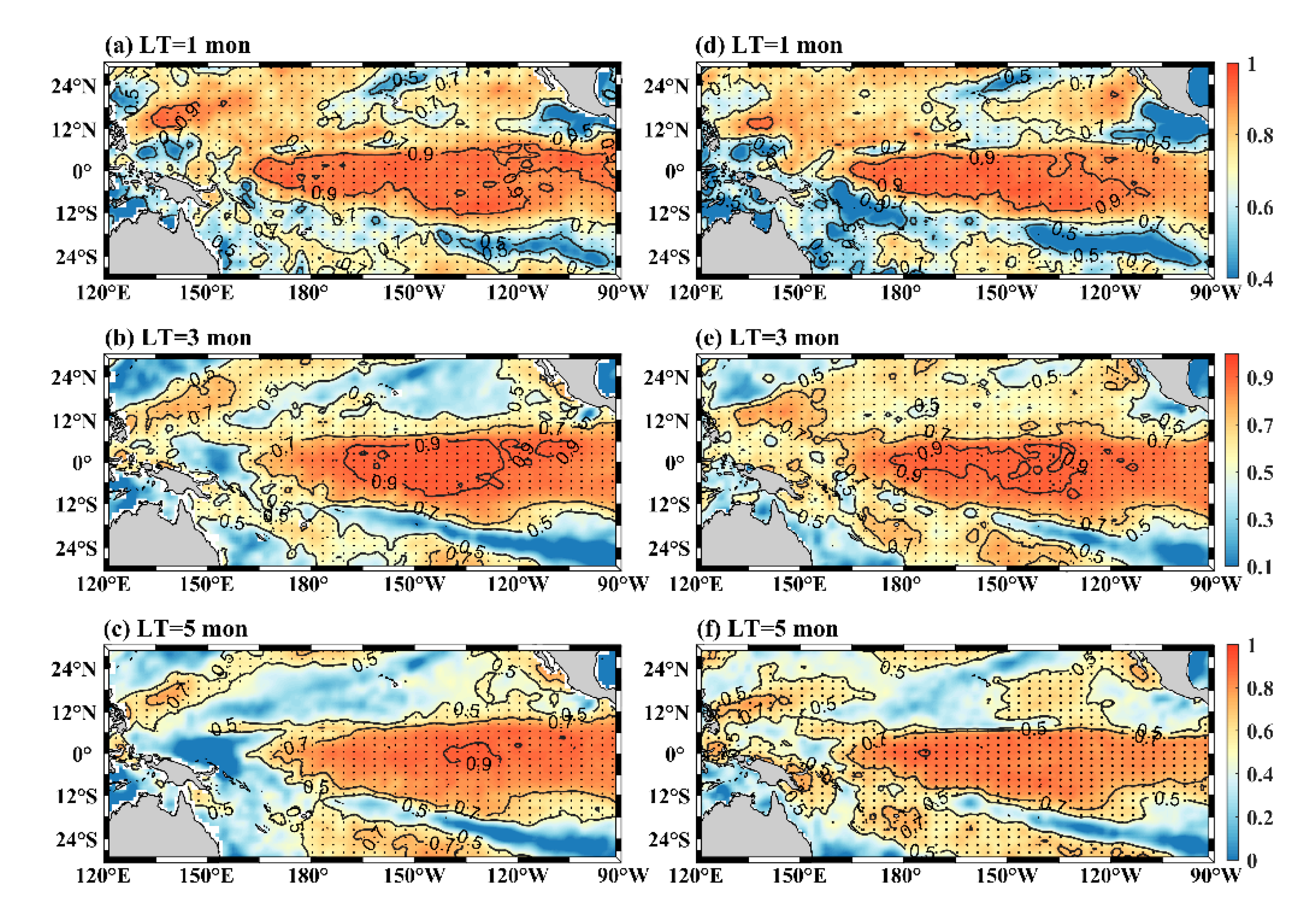
Firstly, the winter ACC spatial pattern in the tropical Pacific Ocean is investigated (Figure 1). For the modified FIO-ESM-CPS, the areas for which predictive skills are highest are located in the tropical central Pacific. There, the values of the ACC are over 0.9 at a 1-month lead time. The results of original FIO-ESM-CPS are similar, which means that both modified and original FIO-ESM-CPS can skillfully predict winter SST anomalies associated with ENSO when initialized from a 1-month lead. Meanwhile, with the increasing of lead months, the ACCs of both forecast systems decrease. As compared with the original CGCM, the ACC of the modified FIO-ESM-CPS decreases at a slower rate. In the results of FIO-ESM-CPS, many more ACCs have negative values at a 5-month lead time.
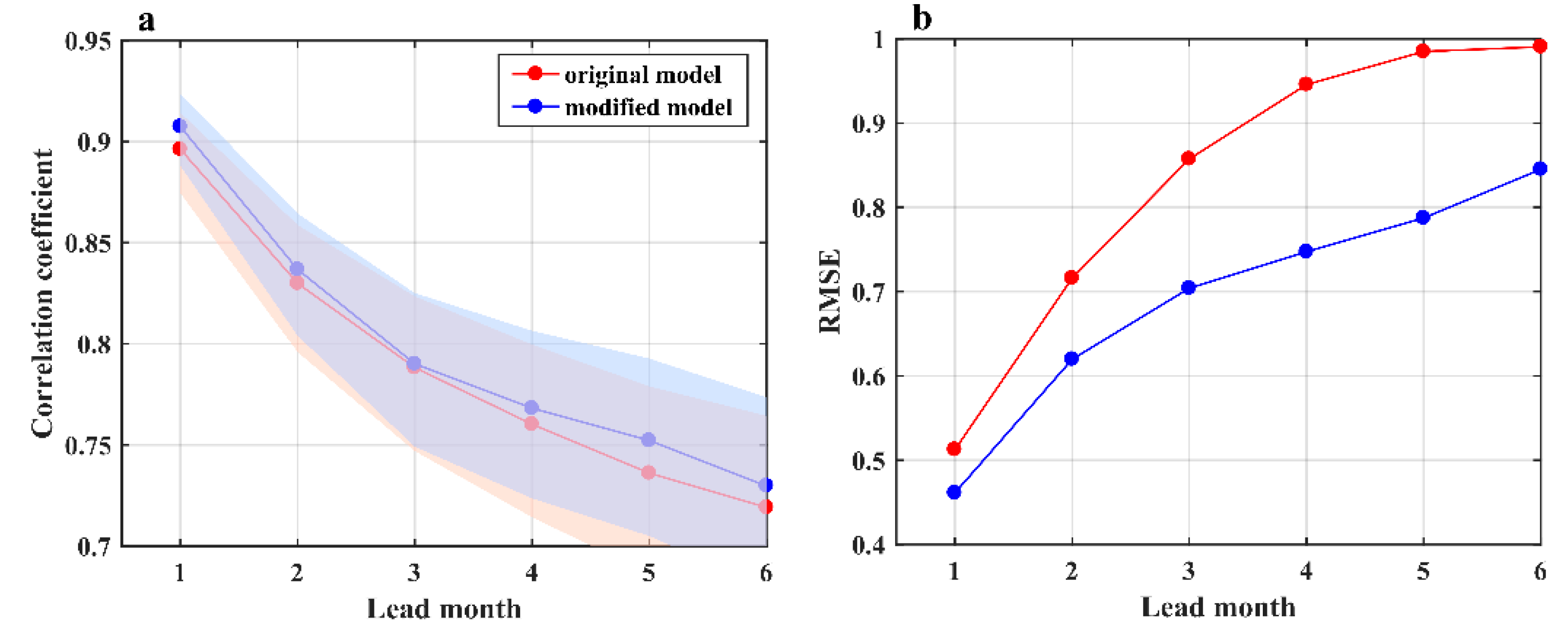
The seasonal prediction results of ACC and RMSE of Niño 3.4 index from lead 1-month to lead 6-month are shown in Figure 2. There, the ACC between the modified FIO-ESM-CPS and observations is clearly larger than that for the original CGCM (Figure 2a), which implies that ENSO prediction skill has improved. From the 1- to 6-month lead times, the skillful prediction of ENSO as represented by ACC continues to decrease. At the 1-, 2-, and 3-month lead times, the two ACCs are similar. At the 5-month lead time, the difference of ACC between the modified and original FIO-ESM-CPS is largest, changing from 0.7522 to 0.7361, an increase of 2.2%. The RMSE has also been improved (Figure 2b). The values of RMSE of modified FIO-ESM-CPS are all significantly smaller than that of the original CGCM from the 1-month to 6-month lead times. The RMSE of original FIO-ESM-CPS sharply increases from 0.512 at the 1-month lead to 0.990 at the 6-month lead. However, the rate of the error growth of RMSE is slower. At the 1-month lead time, the RMSE is 0.461, increasing to 0.845 at the 6-month lead. The largest improvement of RMSE appears at the 4-month lead time. The amplitude decreases by 21%.
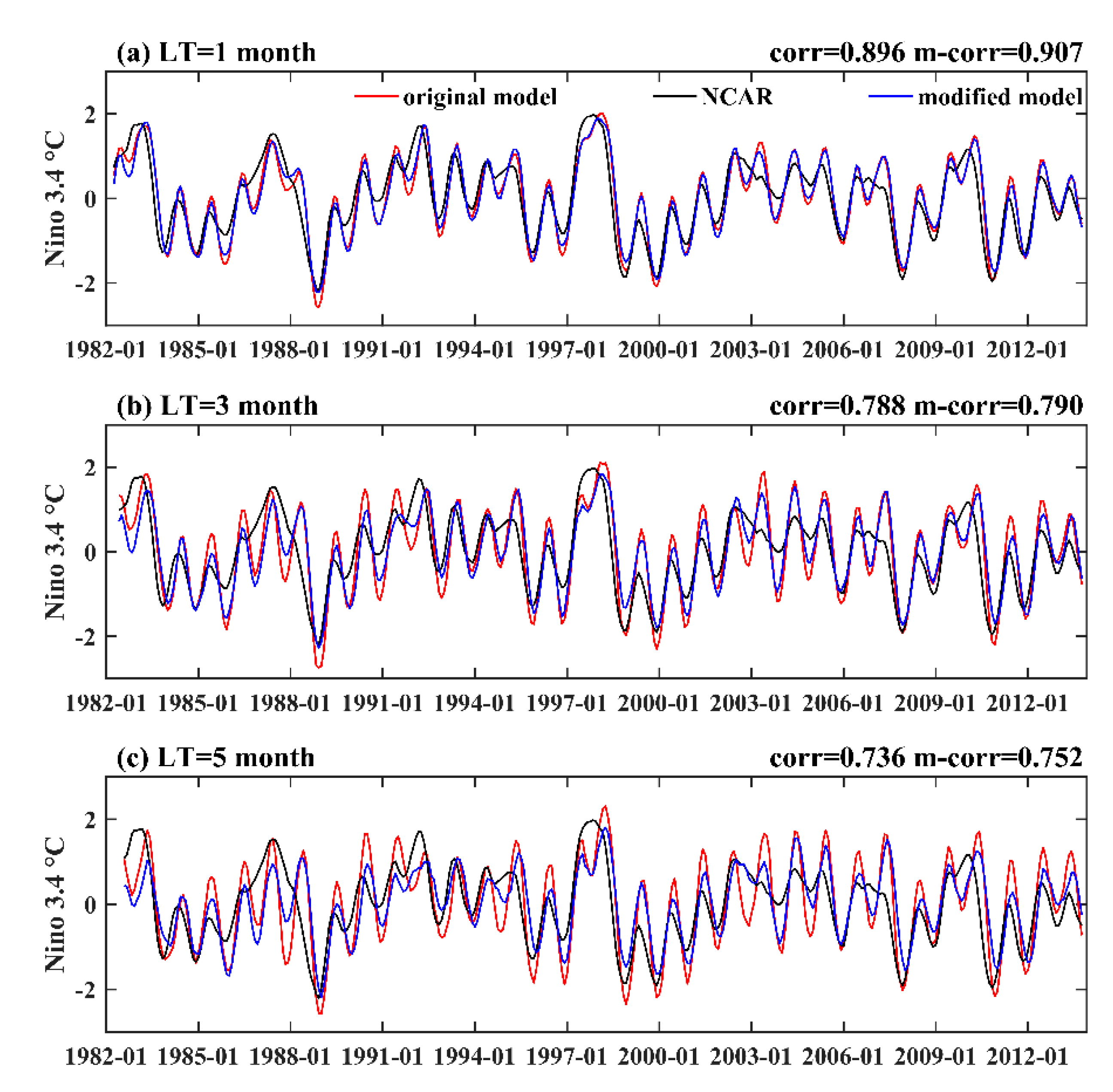
Next, the time series of Niño 3.4 index of the two forecasting systems and observations at the 1-, 3-, and 5-month lead times are shown in Figure 3. Consistent with the results of Figure 2, the three time series match well at the 1-month lead time. Over longer lead times, results sour. At a 5-month lead time, the amplitude of the two forecasting systems is significantly larger than the observations. As in previous studies, neither the original nor modified model can skillfully prediction the ENSO amplitude [17]. In comparing the original and modified FIO-ESM-CPS CGCMs, closer agreement with the Niño 3.4 index observations occurs for the modified model.
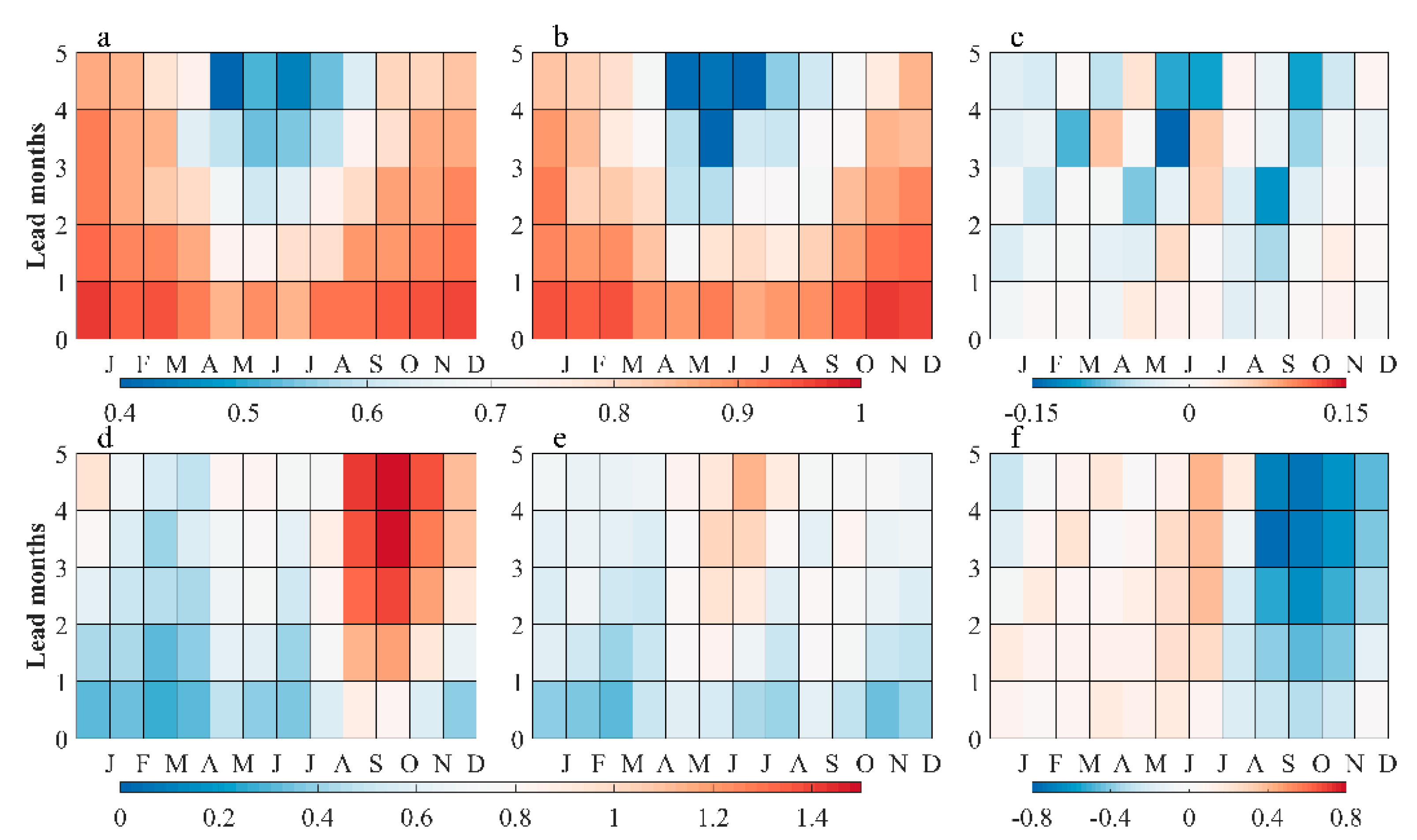
Figure 4 shows the forecast skill for the RMSE and ACC of Niño 3.4 index of the predicted target month and lead time. The distribution patterns of ACC between modified and original FIO-ESM-CPS both show a gap of lower values in the spring and summer. Thus, the SPB and its persistence still significantly limit the prediction of ENSO. The difference of ACC between modified and original models is slight. At longer lead times, improvements in RMSE generally occur from July to December.
3.2. PDO Prediction Skill Evaluation
To evaluate the prediction of PDO, the ACC of the PDO index and RMSE between model results and observation are estimated. The results show that the prediction skill of PDO is improved significantly (Figure 5). At 1-year and 2-year lead time, the original FIO-ESM-CPS shows very poor prediction with the ACC less than 0.1, while the ACC in the modified one can reach 0.436, significant at 95% confidence level. The most obvious improvement of modified FIO-ESM-CPS is at the 1-year and the 2-year lead time due to poor prediction skill of original one, while the two prediction systems have outstanding prediction skill at longer lead time, especially at 4-year lead. The ACC in modified FIO-ESM-CPS can reach 0.587 and leads to an improvement of 36% as compared to the original model at the 4-year lead time. The RMSE is also improved obviously. The largest reduction of RMSE occurs at the 3-year lead time, which is an improvement of 21% over the original model.
3.3. Possible Reasons for Prediction Skill Improvement
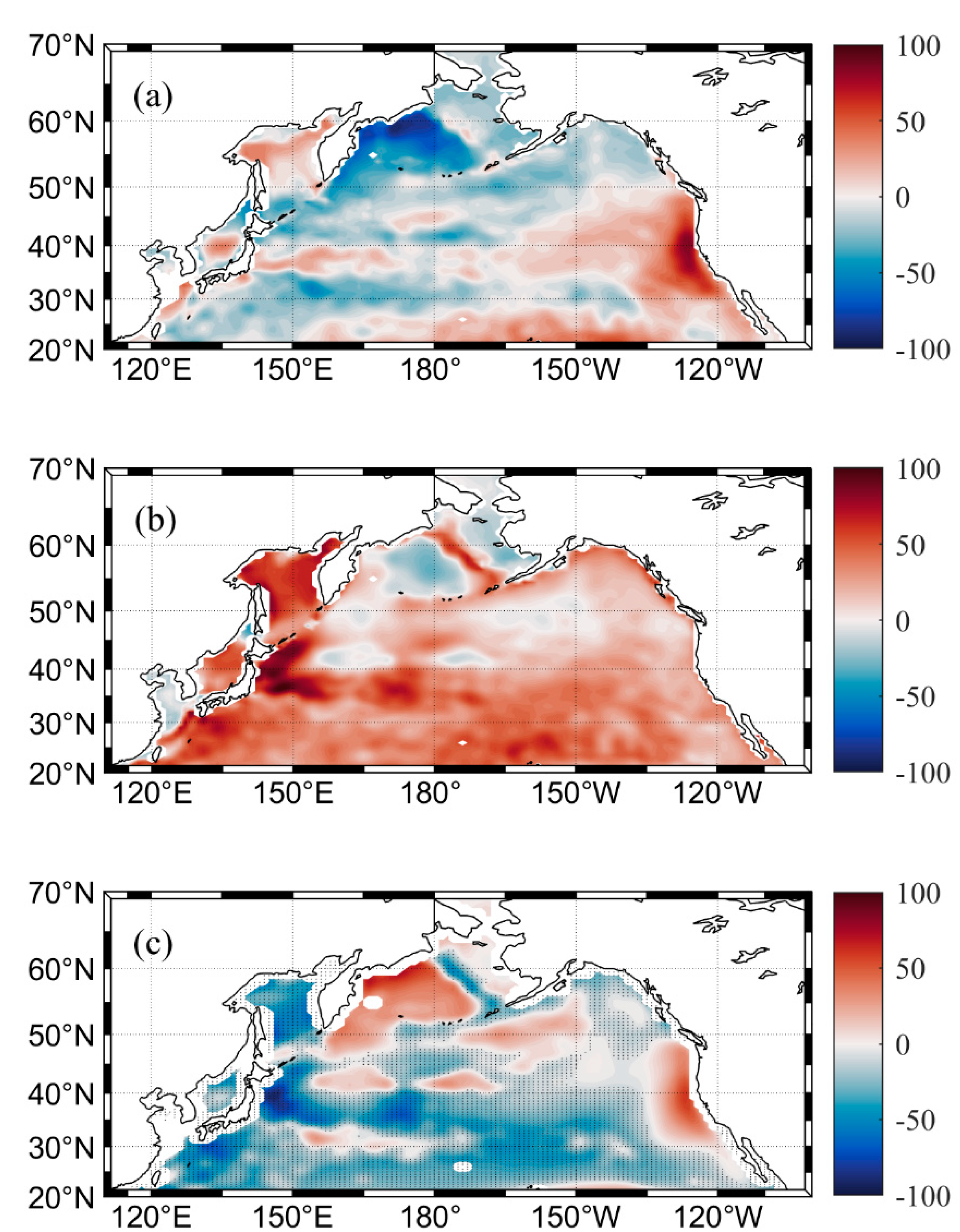
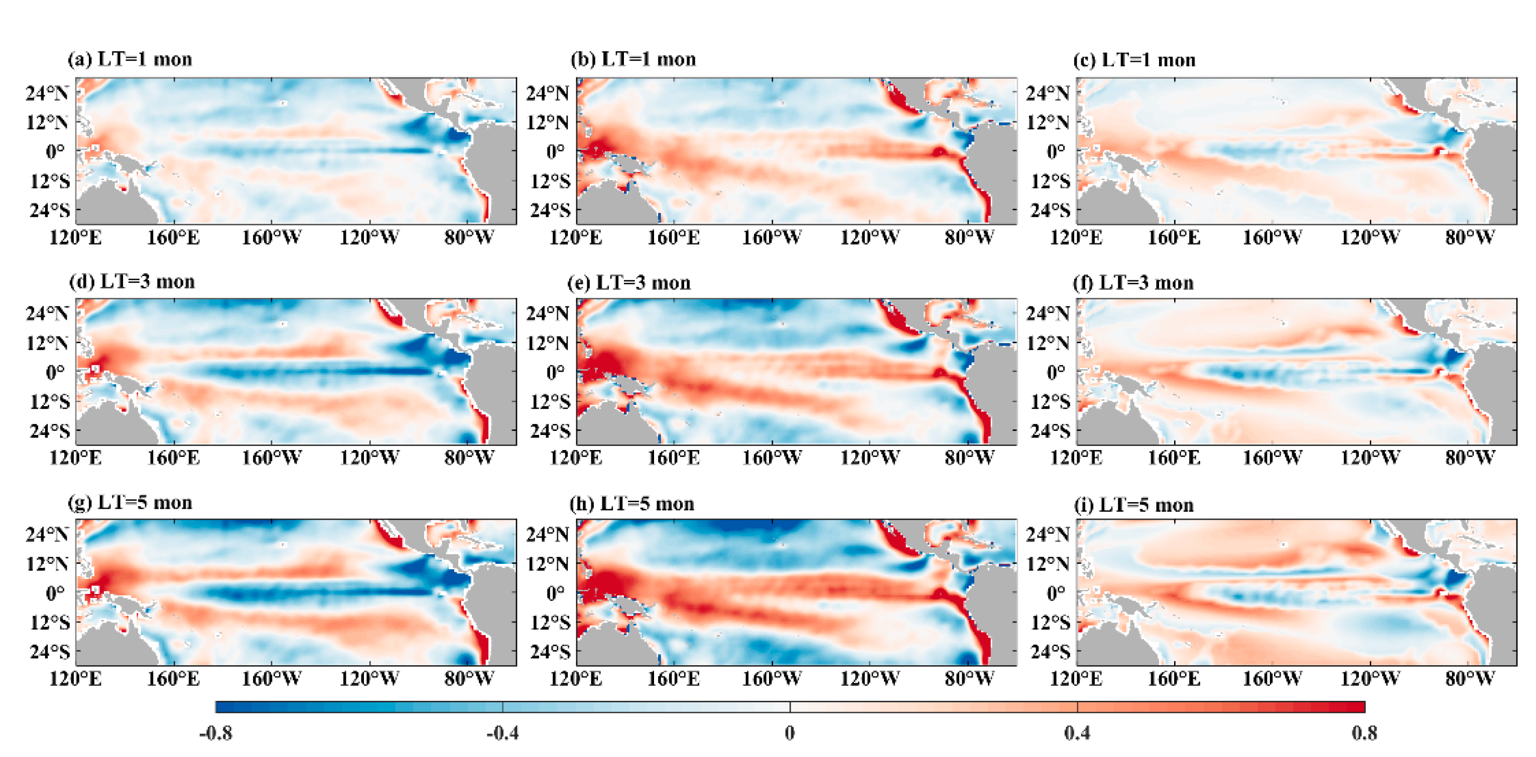
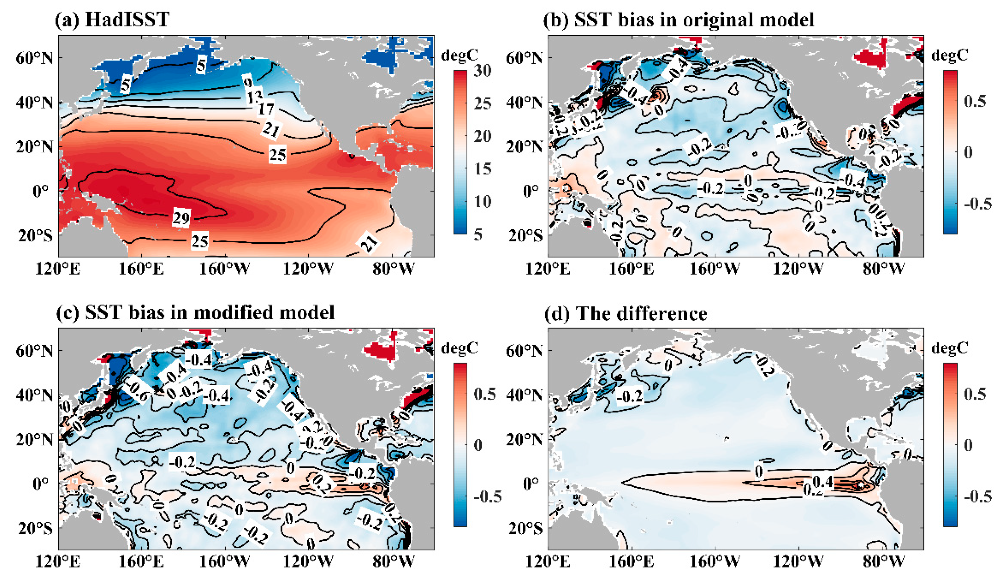
To further investigate possible reasons for improvement of the ENSO prediction skill, the evolution of prediction error of ENSO with change of lead time is shown in Figure 6. With the increasing lead time, prediction errors grow rapidly, especially in the tropical Pacific Ocean. However, there are positive and negative biases, respectively. That may be caused by the bias of climatological simulation of the two models (Figure 7). There, cold tongue biases of the tropical climatological SST within the original model are transformed into a warm tongue in the modified FIO-ESM v2.0. However, the bias of SST in tropical region in simulation of FIO-ESM v2.0 is still cold, so the prediction errors of FIO-ESM-CPS in tropical region are negative. Although the SST biases in the tropical region change from being underestimated in FIO-ESM v2.0 to being overestimated in the modified FIO-ESM v2.0, the absolute average errors in the tropical region in the modified FIO-ESM-CPS are significantly smaller than those in FIO-ESM-CPS (Figure 6). This may be the reason why the ENSO prediction skill improves.
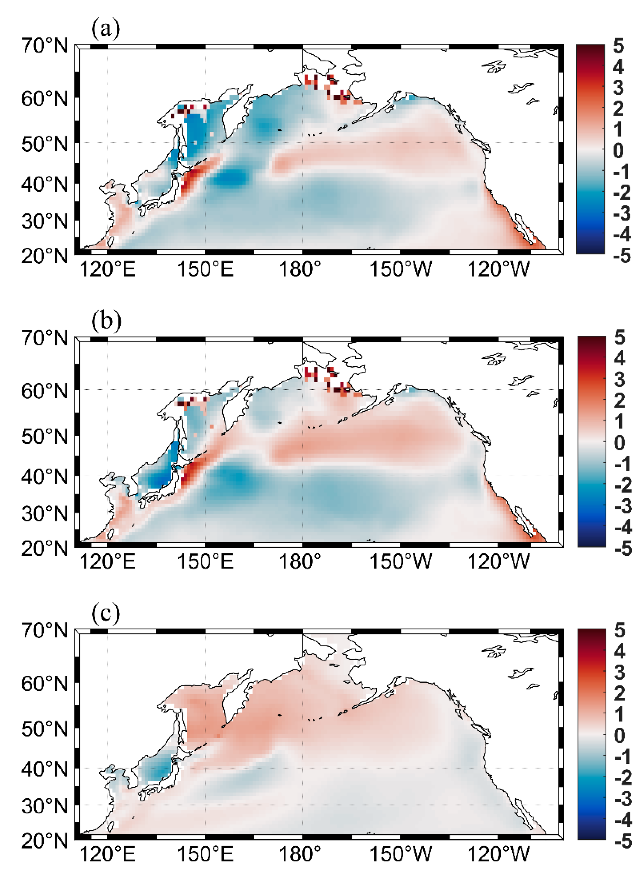
PDO is the dominant internal variability in climate system on a decadal time scale in the NP. To discuss possible reasons for improved PDO prediction skill, an analysis of the prediction SST in NP is needed (Figure 8). The SST biases between prediction and observation show a PDO-like pattern at 1-year lead time. This PDO-like distribution of SST bias is more significant in modified FIO-ESM-CPS. In addition, the PDO-like bias in modified FIO-ESM-CPS can influence the prediction of the intensity of PDO but may be beneficial for PDO predictions.
The mixed layer depths (MLD) are significantly underestimated in most of the models compared with the observation data. Here, we also compare the change of MLD from model output with and without new parameterization schemes. The compiled mixed layer climatology database (MIMOC [66]) is used for comparison. Figure 9a gives the MLD difference between the modified model and MIMOC in the Northern Pacific; the positive bias is present in the Eastern Pacific, and some sporadic positive biases spread out in middle regions between 20° and 40°. In the Northern region, there are obvious negative biases. The original model shows significant positive biases throughout whole Northern Pacific, and shows overestimated MLD. The MLD difference between the modified model and original model is shown in Figure 9c. The modified model shows moderate improvement in some regions. The added wave-induced mixing parameterization deepens MLD, and the SI parameterization scheme is the shoaling of the mixed layer. The joint effect of wave-induced mixing and SI parametrization spatially reduced the MLD when comparing to the original model. Unfortunately, it also further deepens the MLD, especially in coastal regions, where some complicated physical process remain incomprehensible.
4. Discussion
As is well known, the predictive skill is usually affected by initial conditions, model drifts and physical processes. In this study, four new parameterization schemes are introduced into the original FIO-ESM-CPS. These parameterization schemes can modify the turbulences from surface to deep ocean. Although the simulation of climatological SST in the tropical region is overestimated, the cold tongue error is partially alleviated. The new parametrization schemes, which involve two important energy sources (wind and tide) and four physical processes for mixing, help to improve the simulation of mean state by describing the mixing in surface and deep ocean more realistically. Accurate simulation of SST and MLD is key for prediction skill of ENSO and PDO. At the air-sea interface, ocean surface waves play an important role in momentum, energy and gas exchange. The wave-induced mixing improves the excessively high surface temperature simulated in summer and reduces the underestimation of the mixed layer depth in winter as demonstrated by Wang et al. [49]. For improving the SST and MLD simulation, another important submesoscale parameterization scheme (SI parameterization) is included, the primary effect of symmetric instability is the shoaling of the mixed layer. The mixing between mixing layer and ocean interior is driven by internal waves. So, both internal tide and Lee-wave parameterization are considered in the present study. The revised internal tidal mixing parameterization introduces a correction function related to the Coriolis effect on internal tidal local dissipation in the deep ocean based on the original version developed by St. Laurent et al. [55], which is more reasonable via demonstration in laboratory. The Lee-wave parameterization mainly improves the simulations of deep sea water temperature and salinity in seamount-rich areas, and it is a weak contributor for improvements of ENSO and PDO prediction skill. In general, the four parameterization schemes separately present the four important physical process from surface to interior, which has improved the simulation of ocean state to varying degrees, respectively, as demonstrated in the published literature [49,50,51,52]. Improvements in mean state ocean temperature simulations may be responsible for the improvement of prediction skill.
Using a modified FIO-ESM-CPS, the prediction skills for ENSO and PDO are investigated. Two deterministic metrics (ACC and RMSE) are chosen to evaluate the prediction skill. The results show that with the new parameterization schemes, the modified FIO-ESM-CPS shows better prediction. Both modified and original FIO-ESM-CPS have highest ACC and lowest RMSE in the central Pacific in wintertime. It suggests that the two prediction systems have high levels of skill in predicting winter SSTs associated with ENSO at 1-month lead time. Furthermore, the ACC of the Nino 3.4 index between the prediction and observation shows that with the increasing lead time, the prediction skills of the two forecasting systems decrease, but the modified system still has better forecast results. In the modified system, ACCs are slightly higher than that in the original model, with the largest increases of ACC appearing at the 5-month lead time, improving by 2.2%. Moreover, there were also large improvements observed in RMSEs. While original FIO-ESM-CPS forecasts of warm event ENSO amplitudes are significantly larger than the observations, the modified model forecasts are much closer to the observations, with a decrease of 21% being observed at the 4-month lead time. In addition, with the longer lead time, the improvement of RMSE is more significant, especially at 4-, 5- and 6-month lead times. As we know, it is very important to improve predictions at longer lead times. One reason is because with longer lead time, the forecasting is more difficult; the other is because at 6-month lead time forecast can be of benefit for crossing the SPB which is a main barrier to seasonal prediction of ENSO. Despite this advance, the SPB and its persistence is still a challenge to seasonal prediction of ENSO in both forecasting systems. Improvements of PDO prediction skill are also significant for the 1965–2010 period. At 1-year and 2-year lead time the poor prediction of original FIO-ESM-CPS with less than 0.1 for the ACC is changed to be significant at 95% confidence level with the ACC 0.43 in modified model. At 4-year lead time, the ACC improvements can reach 36%, while RMSEs decrease by 21% at 3-year lead time when using the modified FIO-ESM-CPS. At the longer lead time, the prediction of PDO is related to the initialization and external radiative forcing [67]. We would suggest that the improvement of prediction system by finer parameterization is another important factor.
In this study, the significant improvement of seasonal prediction skill of ENSO and year-to-year prediction of PDO are mostly related to the new parameterization schemes introduced to a modified FIO-ESM-CPS. While this study shows the results of just one case, future studies can expand the variables investigated and discuss the effects of multi model ensemble averages that can possibly lead to improvements in ENSO prediction skill.
Author Contributions
Conceptualization, G.L.; methodology, G.L.; software, X.H.; validation, Y.Y.; formal analysis, X.H.; investigation, Y.Y.; resources, X.H., Q.C. and X.W.; data curation, X.H., S.C. and H.G.; writing—original draft preparation, Y.Y.; writing—review and editing, G.L., Q.C., S.C., H.G. and X.W. All authors have read and agreed to the published version of the manuscript.
Funding
This research was funded by the National Key Research and Development Program of China (No. 2017YFA0604100), the National Natural Science Foundation of China (No. 42192562, 42076015, 41676007) and Specific Funding for Natural Resource Development of Jiangsu Province (Oceanic Science and Technology Innovations, JSZRHYKJ202102).
Data Availability Statement
The OISST v2.1 is downloaded from the website https://www.ncei.noaa.gov/products/optimum-interpolation-sst (accessed on 1 December 2021). Sea level anomaly data is acquired from the Archiving, Validation, and Interpretation of Satellite Data (AVISO, https://www.aviso.altimetry.fr/en/data.html accessed on 2 January 2022). The Niño 3.4 and PDO indices used are from the website of NOAA: https://psl.noaa.gov/gcos_wgsp/Timeseries/ (accessed on 1 December 2021). The monthly SST data are from the Hadley Centre Sea Ice and Sea Surface Temperature and the website is https://www.metoffice.gov.uk/hadobs/hadisst/data/download.html (accessed on 1 December 2021).
Acknowledgments
The authors thank Zhenya Song, Yajuan Song and Brandon J. Bethel for their kind help in this work.
Conflicts of Interest
The authors declare no conflict of interest.
References
- Dai, A.G.; Wigley, T.; Boville, B.A.; Kiehl, J.T.; Buja, L.E. Climates of the Twentieth and Twenty-First Centuries Simulated by the NCAR Climate System Model. J. Clim. 2014, 14, 485–519. [Google Scholar] [CrossRef] [Green Version]
- Zhou, T.; Chen, Z.; Zou, L.; Chen, X.; Yu, Y.; Wang, B. Development of Climate and Earth System Models in China: Past Achievements and New Cmip6 Results. J. Meteorol. Res. 2020, 34, 1–19. [Google Scholar] [CrossRef]
- Richter, I. Climate model biases in the eastern tropical oceans: Causes, impacts and ways forward. WIREs Clim. Chang. 2015, 6, 345–358. [Google Scholar] [CrossRef]
- Wang, C.; Zhang, L.; Lee, S.-K.; Wu, L.; Mechoso, C.R. A global perspective on CMIP5 climate model biases. Nat. Clim. Chang. 2014, 4, 201–205. [Google Scholar] [CrossRef]
- Zuidema, P.; Chang, P.; Medeiros, B.; Kirtman, B.P.; Mechoso, R.; Schneider, E.K. Challenges and prospects for reducing coupled climate model SST biases in the eastern tropical Atlantic and Pacific oceans: The U.S. CLIVAR Eastern Tropical Oceans Synthesis Working Group. Bull. Am. Meteorol. Soc. 2016, 97, 2305–2328. [Google Scholar] [CrossRef] [Green Version]
- Zhu, Y.; Zhang, R.-H. Scaling wind stirring effects in an oceanic bulk mixed layer model with application to an OGCM of the tropical Pacific. Clim. Dyn. 2017, 51, 1927–1946. [Google Scholar] [CrossRef] [Green Version]
- Ropelewski, C.F.; Halpert, M.S. Global and regional scale precipitation patterns associated with the El Niño/Southern Oscillation. Mon. Weather Rev. 1987, 115, 1606–1626. [Google Scholar] [CrossRef] [Green Version]
- McPhaden, M.J.; Zebiak, S.E.; Glantz, M.H. ENSO as an integrating concept in earth science. Science 2006, 314, 1740–1745. [Google Scholar] [CrossRef] [Green Version]
- Ashok, K.; Yamagata, T. The El Niño with a difference. Nature 2009, 461, 481–484. [Google Scholar] [CrossRef]
- Mantua, N.J.; Hare, S.R. The Pacific decadal oscillation. J. Ocean 2002, 58, 35–44. [Google Scholar] [CrossRef]
- Newman, M. The Pacific Decadal Oscillation, Revisited. J. Clim. 2016, 29, 4399–4427. [Google Scholar] [CrossRef] [Green Version]
- Wang, L.; Chen, W.; Huang, R. Interdecadal modulation of PDO on the impact of ENSO on the East Asian winter monsoon. Geophys. Res. Lett. 2008, 35, L20702. [Google Scholar] [CrossRef] [Green Version]
- Kim, J.W.; Yeh, S.W.; Chang, E.C. Combined effect of El Nino-Southern Oscillation and Pacific decadal oscillation on the East Asian winter monsoon. Climate Dyn. 2014, 42, 957–971. [Google Scholar] [CrossRef]
- Krishnamurthy, L.; Krishnamurthy, V. Influence of PDO on South Asian summer monsoon and monsoon–ENSO relation. Climate Dyn. 2014, 42, 2397–2410. [Google Scholar] [CrossRef]
- Kayano, M.T.; Andreoli, R.V. Relations of South American summer rainfall interannual variations with the Pacific decadal oscillation. Int. J. Climatol. 2007, 27, 531–540. [Google Scholar] [CrossRef]
- Luo, J.J.; Lee, J.Y.; Yuan, C.X. Current status of intraseasonal–seasonal-to-interannual prediction of the Indo-Pacific climate. In Indo-Pacific Climate Variability and Predictability; Behera, S.K., Yamagata, T., Eds.; World Scientific: Singapore, 2016; pp. 63–107. [Google Scholar]
- Tang, Y.; Zhang, R.H.; Liu, T.; Duan, W.; Yang, D.; Zheng, F.; Ren, H.; Lian, T.; Gao, C.; Chen, D.; et al. Progress in ENSO prediction and predictability study. Natl. Sci. Rev. 2018, 5, 826–839. [Google Scholar] [CrossRef]
- Wang, C. A review of ENSO theories. Natl. Sci. Rev. 2018, 5, 813–825. [Google Scholar] [CrossRef]
- Mantua, N.J.; Hare, S.R.; Zhang, Y.; Wallace, J.M.; Francis, R.C. A Pacific Interdecadal Climate Oscillation with Impacts on Salmon Production. Bull. Am. Meteor. Soc. 1997, 78, 1069–1080. [Google Scholar] [CrossRef]
- Cassou, C.; Kushnir, Y.; Hawkins, E.; Pirani, A.; Kucharski, F.; Kang, I.-S.; Caltabiano, N. Decadal climate variability and predictability: Challenges and opportunities. Bull. Am. Meteorol. Soc. 2018, 99, 479–490. [Google Scholar] [CrossRef] [Green Version]
- Song, Y.J.; Shu, Q.; Bao, Y. The Short-Term Climate Prediction System FIO-CPS v2.0 and its Prediction Skill in ENSO. Front. Earth Sci. 2021, 9, 950. [Google Scholar] [CrossRef]
- Zhang, S.; Liu, Z.; Zhang, X.; Wu, X.; Han, G.; Zhao, Y. Coupled Data Assimilation and Parameter Estimation in Coupled Ocean-Atmosphere Models: A Review. Clim. Dyn. 2020, 54, 5127–5144. [Google Scholar] [CrossRef]
- Hu, Z.Z.; Kumar, A.; Huang, B.; Zhu, J.; Guan, Y. Prediction Skill of north Pacific Variability in NCEP Climate Forecast System Version 2: Impact of ENSO and beyond. J. Clim. 2014, 27, 4263–4272. [Google Scholar] [CrossRef] [Green Version]
- Zhu, J.; Kumar, A.; Wang, W.; Hu, Z.Z.; Huang, B.; Balmaseda, M.A. Importance of Convective Parameterization in ENSO Predictions. Geophys. Res. Lett. 2017, 44, 6334–6342. [Google Scholar] [CrossRef]
- Barnston, A.G.; Tippett, M.K.; L’Heureux, M.L.; Li, S.; DeWitt, D.G. Skill of real-time seasonal ENSO model predictions during 2002–11: Is our capability increasing? Bull. Amer. Meteor. Soc. 2012, 93, 631–651. [Google Scholar] [CrossRef]
- Zheng, Z.; Hu, Z.Z.; L’Heureux, M. Predictable components of ENSO evolution in real-time multi-model predictions. Sci. Rep. 2016, 6, 35909. [Google Scholar] [CrossRef] [PubMed] [Green Version]
- Zhang, R.H.; Gao, C. The IOCAS intermediate coupled model (IOCASICM) and its real-time predictions of the 2015–2016 El Niño event. Sci. Bull. 2016, 61, 1061–1070. [Google Scholar] [CrossRef] [Green Version]
- Samelson, R.M.; Tziperman, E. Instability of the chaotic ENSO: The growth-phase predictability barrier. J. Atmos. Sci. 2001, 58, 3613–3625. [Google Scholar] [CrossRef] [Green Version]
- McPhaden, M.J. Tropical Pacific Ocean heat content variations and ENSO persistence barriers. Geophys. Res. Lett. 2003, 30, 1480. [Google Scholar] [CrossRef] [Green Version]
- Mu, M.; Duan, W.S.; Wang, B. Season-dependent dynamics of non-linear optimal error growth and El Niño-Southern Oscillation predict-ability in a theoretical model. J. Geophys. Res. 2007, 112, D10113. [Google Scholar]
- Duan, W.S.; Liu, X.C.; Zhu, K.Y.; Mu, M. Exploring the initial errors that cause a significant “spring predictability barrier” for El Niño events. J. Geophys. Res. 2009, 114, C04022. [Google Scholar] [CrossRef] [Green Version]
- Yu, Y.S.; Mu, M.; Duan, W.S. Does model parameter error cause a significant “Spring Predictability Barrier” for El Niño events in the Zebiak-Cane model? J. Clim. 2012, 25, 1263–1277. [Google Scholar] [CrossRef]
- Fang, X.H.; Mu, M. A three-region conceptual model for central Pacific El Niño including zonal advective feedback. J. Clim. 2018, 31, 4965–4979. [Google Scholar] [CrossRef]
- Imada, Y.; Tatebe, H.; Ishii, M.; Chikamoto, Y.; Mori, M.; Arai, M.; Watanabe, M.; Kimoto, M. Predictability of two types of El Niño assessed using an extended seasonal prediction system by MIROC. Mon. Weather Rev. 2015, 143, 4597–4617. [Google Scholar] [CrossRef]
- Meehl, G.A.; Hu, A.; Teng, H. Initialized decadal prediction for transition to positive phase of the interdecadal Pacific oscillation. Nat. Commun. 2016, 7, 11718. [Google Scholar] [CrossRef] [PubMed] [Green Version]
- Mehta, V.M.; Mendoza, K.; Wang, H. Predictability of phases and magnitudes of natural decadal climate variability phenomena in CMIP5 experiments with the UKMO HadCM3, GFDL-CM2.1, NCAR-CCSM4, and MIROC5 global earth system models. Clim. Dyn. 2019, 52, 3255–3275. [Google Scholar] [CrossRef] [PubMed] [Green Version]
- Wiegand, K.N.; Brune, S.; Baehr, J. Predictability of multiyear trends of the Pacific Decadal Oscillation in an MPI-ESM hindcast ensemble. Geophy. Res. Lett. 2019, 46, 318–325. [Google Scholar] [CrossRef] [Green Version]
- Boer, G.J.; Sospedra-Alfonso, R. Assessing the skill of the Pacific Decadal Oscillation (PDO) in a decadal prediction experiment. Clim. Dyn. 2019, 53, 5763–5775. [Google Scholar] [CrossRef] [Green Version]
- Jochum, M.; Briegleb, B.P.; Danabasoglu, G.; Large, W.G.; Norton, N.J.; Jayne, S.R. The impact of oceanic near-inertial waves on climate. J. Clim. 2013, 26, 2833–2844. [Google Scholar] [CrossRef] [Green Version]
- Melet, A.; Hallberg, R.; Legg, S.; Polzin, K. Sensitivity of the ocean state to the vertical distribution of internal-tide-driven mixing. J. Phys. Oceanogr. 2013, 43, 602–615. [Google Scholar] [CrossRef] [Green Version]
- Zhang, R.H.; Zebiak, S.E. An embedding method for improving interannual variability simulations in a hybrid coupled model of the tropical Pacific Ocean-atmosphere system. J. Clim. 2004, 17, 2794–2812. [Google Scholar] [CrossRef]
- Bao, Y.; Song, Z.; Qiao, F. FIO-ESM Version 2.0: Model Description and Evaluation. J. Geophys. Res. Oceans 2020, 125, e2019JC016036. [Google Scholar] [CrossRef]
- Neale, R.B.; Chen, C.C.; Gettelman, A.; Lauritzen, P.H.; Park, S.; Williamson, D.L. Description of the NCAR Community Atmosphere Model (CAM5.0); NCAR Technical Note TN-486+STR; National Center for Atmospheric Research: Boulder, CO, USA, 2010. [Google Scholar]
- Lawrence, D.M.; Oleson, K.W.; Flanner, M.G.; Thornton, P.E.; Swenson, S.C.; Lawrence, P.J. Parameterization improvements and functional and structural advances in version 4 of the community land model. J. Adv. Model. Earth Syst. 2011, 3, M03001. [Google Scholar] [CrossRef]
- Qiao, F.; Song, Z.; Bao, Y.; Song, Y.; Shu, Q.; Huang, C.; Zhao, W. Development and evaluation of an Earth System Model with surface gravity waves. J. Geophys. Res. Ocean. 2013, 118, 4514–4524. [Google Scholar] [CrossRef]
- Qiao, F.; Zhao, W.; Yin, X.; Huang, X.; Liu, X.; Shu, Q. A Highly Effective Global Surface Wave Numerical Simulation with Ultra-High Resolution. In Proceedings of the International Conference for High Performance Computing, Networking, Storage and Analysis (SC ‘16), Piscataway, NJ, USA, 13–18 November 2016. [Google Scholar]
- Hunke, E.C.; Lipscomb, W.H. CICE: The Los Alamos Sea Ice Model. Documentation and Software User’s Manual; Version 4.0, Tech. Rep. LA-CC-06-012; T-3 Fluid Dynamics Group, Los Alamos National Laboratory: Los Alamos, NM, USA, 2008. [Google Scholar]
- Large, W.G.; McWilliams, J.C.; Doney, S.C. Oceanic vertical mixing: A review and a model with a nonlocal boundary layer parameterization. Rev. Geophys. 1994, 32, 363–403. [Google Scholar] [CrossRef] [Green Version]
- Wang, H.; Dong, C.; Fox-Kemper, B.; Li, Q.; Yang, Y.; Chen, X.; Kenny, T.C.; Sian, L.K. Parameterization of Ocean Surface Wave-Induced Mixing Using Large Eddy Simulations (LES) II. Deep Sea Res. Part II, 2022; submitted. [Google Scholar]
- Cao, Q.; Dong, C.; Ji, Y.; Jiang, X.; Bethel, B.J.; Xia, C. Seamount-Induced Mixing Revealed through Idealized Experiments and its Parameterization in OGCM. Deep Sea Res. Part II 2022, 2022, 105144. [Google Scholar] [CrossRef]
- Tan, J.; Chen, X.; Meng, J.; Liao, G.; Hu, X.; Du, T. A New Parameterization of Internal Tidal Mixing in the Deep Ocean Based on Rotation Experiments. Deep Sea Res. Part II Top. Stud. Oceanogr. 2022, 2022, 105141. [Google Scholar] [CrossRef]
- Dong, J.; Fox-Kemper, B.; Zhu, J.; Dong, C. Application of symmetric instability parameterization in the Coastal and Regional Ocean Community Model (CROCO). J. Adv. Model. Earth Syst. 2020, 13, e2020MS002302. [Google Scholar] [CrossRef]
- Harcourt, R.R.; D’Asaro, E.A. Large-eddy simulation of Langmuir turbulence in pure wind seas. J. Phys. Oceanogr. 2008, 38, 1542–1562. [Google Scholar] [CrossRef]
- Large, W.G.; Pond, S. Sensible and Latent Heat Flux Measurements over the Ocean. J. Phys. Oceanogr. 1982, 12, 464–482. [Google Scholar] [CrossRef] [Green Version]
- St. Laurent, L.C.; Simmons, H.L.; Jayne, S.R. Estimating tidally driven mixing in the deep ocean. Geophys. Res. Lett. 2002, 29, 21. [Google Scholar]
- Jayne, S.R. The impact of abyssal mixing parameterizations in an ocean general circulation model. J. Phys. Oceanogr. 2009, 39, 1756–1775. [Google Scholar] [CrossRef]
- Li, Y.; Xu, Y. Penetration depth of diapycnal mixing generated by wind stress and flow over topography in the northwestern Pacific. J. Geophys. Res. Ocean 2014, 119, 5501–5514. [Google Scholar] [CrossRef]
- Bachman, S.D.; Fox-Kemper, B.; Taylor, J.R.; Thomas, L.N. Parameterization of frontal symmetric instabilities. I: Theory for resolved fronts. Ocean Model. 2017, 109, 72–95. [Google Scholar] [CrossRef]
- Thomas, L.N.; Taylor, J.R.; Ferrari, R.; Joyce, T.M. Symmetric instability in the Gulf Stream. Deep Sea Res. Part II 2013, 91, 96–110. [Google Scholar] [CrossRef]
- Thomas, L.N. Destruction of potential vorticity by winds. J. Phys. Oceanogr. 2005, 35, 2457–2466. [Google Scholar] [CrossRef]
- Anderson, P.S. Measurement of Prandtl number as a function of Richardson number avoiding self-correlation. Boundary-Layer Meteorology 2009, 131, 345–362. [Google Scholar] [CrossRef]
- Banzon, V.; Smith, T.M.; Steele, M.; Huang, B.; Zhang, H.-M. Improved Estimation of Proxy Sea Surface Temperature in the Arctic. J. Atmos. Ocean. Technol. 2020, 37, 341–349. [Google Scholar] [CrossRef]
- Ducet, N.; Le Traon, P.Y.; Reverdin, G. Global High-Resolution Mapping of Ocean Circulation from TOPEX/Poseidon and ERS-1 and 2. J. Geophys. Res. 2000, 105, 19477–19498. [Google Scholar] [CrossRef]
- Reynolds, R.W.; Smith, T.M.; Liu, C.; Chelton, D.B.; Casey, K.S.; Schlax, M.G. Daily High-Resolution-Blended Analyses for Sea Surface Temperature. J. Clim. 2007, 20, 5473–5496. [Google Scholar] [CrossRef]
- Rayner, N.A.; Parker, D.E.; Horton, E.B. Global analyses of sea surface temperature, sea ice, and night marine air temperature since the late nineteenth century. J. Geophys. Res. Atmos. 2003, 108, 4407. [Google Scholar] [CrossRef]
- Holte, J.; Talley, L.D.; Gilson, J.; Roemmich, D. An Argo mixed layer climatology and database. Geophys. Res. Lett. 2017, 44, 5618–5626. [Google Scholar] [CrossRef] [Green Version]
- Choi, J.; Son, S.-W. Seasonal-to-decadal prediction of El Niño–Southern Oscillation and Pacific Decadal Oscillation. npj Clim. Atmos. Sci. 2022, 5, 29. [Google Scholar] [CrossRef]
Figure 1.
Spatial distribution of temporal correlation predictive skill scores (shading, unit: 1) of the boreal winter SSTAs at (a,d) 1-month, (b,e) 3-month, and (c,f) 5-month lead times for FIO−ESM−CPS (left panels), for modified FIO−ESM−CPS (right panels). Stipples denote values passing the 1% significance level.

Figure 2.
The ACC (a) with the shaded area indicating the 95% confidence interval and RMSE (b) of the Niño 3.4 index between the observation and the prediction for 1982–2013. The red and blue lines represent the observation and predicted results of original and modified FIO−ESM−CPS for 1− to 6−month lead times (unit: 1).

Figure 3.
Time series of Niño 3.4 index values predicted by observation (black), FIO−ESM−CPS (red line) and modified FIO−ESM−CPS (blue line) at (a) 1-, (b) 3-, and (c) 5-month lead times (unit: 1).
Figure 3.
Time series of Niño 3.4 index values predicted by observation (black), FIO−ESM−CPS (red line) and modified FIO−ESM−CPS (blue line) at (a) 1-, (b) 3-, and (c) 5-month lead times (unit: 1).

Figure 4.
The ACC and RMSE of the Niño 3.4 index forecast skill for all the target months and lead months obtained using the FIO−ESM−CPS (a,d); modified FIO−ESM−CPS (b,e); the differences between modified and original FIO−ESM−CPS (c,f) (unit: 1).
Figure 4.
The ACC and RMSE of the Niño 3.4 index forecast skill for all the target months and lead months obtained using the FIO−ESM−CPS (a,d); modified FIO−ESM−CPS (b,e); the differences between modified and original FIO−ESM−CPS (c,f) (unit: 1).

Figure 5.
The (a) ACC with the shaded area in indicating the 95% confidence interval and (b) RMSE of the PDO index between the observation and the prediction for 1965–2010. The red and blue lines represent the observation and predicted results of original and modified FIO−ESM−CPS for 1- to 4-year lead times (unit: 1).
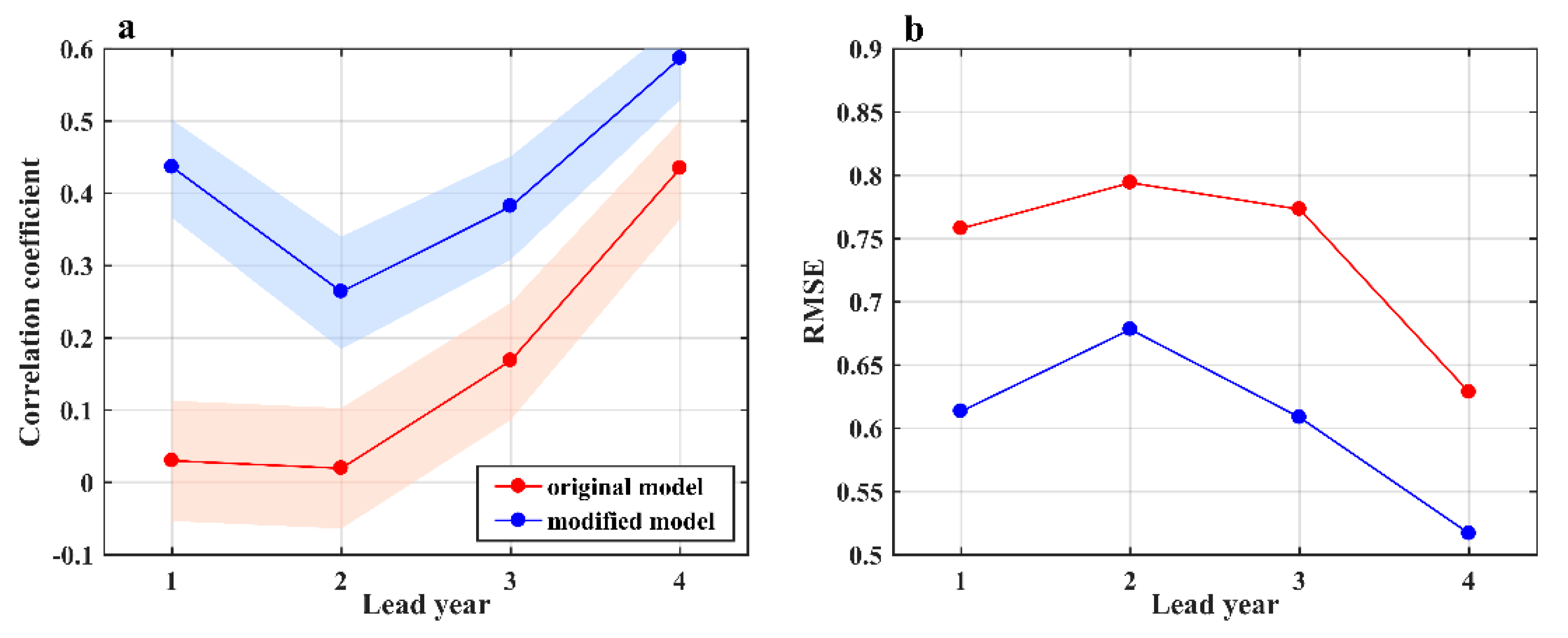
Figure 6.
Spatial patterns of SSTA biases (units: °C) between the predictions and observation: FIO−ESM−CPS results (a,d,g), modified FIO−ESM−CPS results (b,e,h). The difference of absolute average error between modified and original FIO−ESM−CPS (c,f,i). (a–c) 1-month lead time, (d–f) 3-month lead time, and (g–i) 5-month lead time.

Figure 7.
The climatological SST ((a), units: °C), SST biases in original (b), modified FIO−ESM−CPS (c) and the difference of SST biases between modified and original FIO−ESM−CPS (d).
Figure 7.
The climatological SST ((a), units: °C), SST biases in original (b), modified FIO−ESM−CPS (c) and the difference of SST biases between modified and original FIO−ESM−CPS (d).

Figure 8.
Spatial patterns of SSTA biases in north Pacific (units: °C) between the predictions and observation: (a) original FIO−ESM−CPS results, (b) modified FIO−ESM−CPS results, and (c) the difference of bias between modified and original FIO-ESM-CPS at 1-year lead time.
Figure 8.
Spatial patterns of SSTA biases in north Pacific (units: °C) between the predictions and observation: (a) original FIO−ESM−CPS results, (b) modified FIO−ESM−CPS results, and (c) the difference of bias between modified and original FIO-ESM-CPS at 1-year lead time.

Figure 9.
Spatial patterns of mixed layer depth biases in north Pacific (units: °C) in winter (DJF) between the predictions and observation: (a) modified FIO−ESM−CPS results, (b) original FIO−ESM−CPS results, and (c) the difference of absolute average error between modified and original FIO−ESM−CPS at 1-year lead time. Stipples denote the improvement of absolute average error between modified and original FIO−ESM−CPS over 20%.

Table 1.
Experimental Design.
| CONTROL | SENSI | ||
|---|---|---|---|
| Historical Assimilation Experiment | Time | 1961–2016 | 1961–2016 |
| Assimilation Data | 1961–1982: COBE SST1982–2016: AVHRR SST | 1961–1982: COBE SST1982–2016: AVHRR SST | |
| ENSO Prediction Experiment | Time | 1982–2016 | 1982–2016 |
| Start time | 1st of every month | 1st of every month | |
| Predicted time | 7 months | 7 months | |
| PDO Prediction Experiment | Time | 1961–2016 | 1961–2016 |
| Start time | 1 November every year | 1 November every year | |
| Predicted time | 5 years | 5 years |
Publisher’s Note: MDPI stays neutral with regard to jurisdictional claims in published maps and institutional affiliations. |
© 2022 by the authors. Licensee MDPI, Basel, Switzerland. This article is an open access article distributed under the terms and conditions of the Creative Commons Attribution (CC BY) license (https://creativecommons.org/licenses/by/4.0/).
Share and Cite
MDPI and ACS Style
Yang, Y.; Hu, X.; Liao, G.; Cao, Q.; Chen, S.; Gao, H.; Wei, X. Improved ENSO and PDO Prediction Skill Resulting from Finer Parameterization Schemes in a CGCM. Remote Sens. 2022, 14, 3363. https://doi.org/10.3390/rs14143363
AMA Style
Yang Y, Hu X, Liao G, Cao Q, Chen S, Gao H, Wei X. Improved ENSO and PDO Prediction Skill Resulting from Finer Parameterization Schemes in a CGCM. Remote Sensing. 2022; 14(14):3363. https://doi.org/10.3390/rs14143363
Chicago/Turabian StyleYang, Yuxing, Xiaokai Hu, Guanghong Liao, Qian Cao, Sijie Chen, Hui Gao, and Xiaowei Wei. 2022. "Improved ENSO and PDO Prediction Skill Resulting from Finer Parameterization Schemes in a CGCM" Remote Sensing 14, no. 14: 3363. https://doi.org/10.3390/rs14143363
Note that from the first issue of 2016, this journal uses article numbers instead of page numbers. See further details here.