
Estimation of Grapevine Crop Coefficient Using a Multispectral Camera on an Unmanned Aerial Vehicle


1
School of Agriculture, Food and Wine, The University of Adelaide, PMB 1, Glen Osmond, SA 5064, Australia
2
Research Institute for the Environment and Livelihoods, Charles Darwin University, Casuarina, NT 0810, Australia
3
Oliphant Building, North Terrace Campus, School of Biological Science, The University of Adelaide, Adelaide, SA 5005, Australia
*
Author to whom correspondence should be addressed.
Remote Sens. 2021, 13(13), 2639; https://doi.org/10.3390/rs13132639
Submission received: 19 April 2021
/
Revised: 26 June 2021
/
Accepted: 28 June 2021
/
Published: 5 July 2021
(This article belongs to the Special Issue Remote Sensing for Crop Water Stress Detection and Irrigation Management)
Abstract
:Crop water status and irrigation requirements are of great importance to the horticultural industry due to changing climatic conditions leading to high evaporative demands, drought and water scarcity in semi-arid and arid regions worldwide. Irrigation scheduling strategies based on evapotranspiration (ET), such as regulated deficit irrigation, requires the estimation of seasonal crop coefficients (kc). The ET-driven irrigation decisions for grapevines rely on the sampling of several kc values from each irrigation zone. Here, we present an unmanned aerial vehicle (UAV)-based technique to estimate kc at the single vine level in order to capture the spatial variability of water requirements in a commercial vineyard located in South Australia. A UAV carrying a multispectral sensor is used to extract the spectral, as well as the structural, information of Cabernet Sauvignon grapevines. The spectral and structural information, acquired at the various phenological stages of the vine through two seasons, is used to model kc using univariate (simple linear), multivariate (generalised linear and additive) and machine learning (convolution neural network and random forest) model frameworks. The structural information (e.g., canopy top view area) had the strongest correlation with kc throughout the season (p ≤ 0.001; Pearson R = 0.56), while the spectral indices (e.g., normalised indices) turned less-sensitive post véraison—the onset of ripening in grapes. Combining structural and spectral information improved the model’s performance. Among the investigated predictive models, the random forest predicted kc with the highest accuracy (R2: 0.675, root mean square error: 0.062, and mean absolute error: 0.047). This UAV-based approach improves the precision of irrigation by capturing the spatial variability of kc within a vineyard. Combined with an energy balance model, the water needs of a vineyard can be computed on a weekly or sub-weekly basis for precision irrigation. The UAV-based characterisation of kc can further enhance the water management and irrigation zoning by matching the infrastructure with the spatial variability of the irrigation demand.
1. Introduction
Water availability to horticultural crops in Australia is highly variable from season-to-season due to variable climatic conditions including evapotranspiration and precipitation patterns, extreme weather events, for example, heatwaves, and competing demand for freshwater. Climatic conditions are expected to deteriorate due to variability in the Indian Ocean Dipole, which is the key driver of ENSO outlook and the Australian climate [1,2]. The persistent drier conditions, combined with freshwater scarcities, will require a wider adaptation of precision irrigation to sustain the horticulture and agriculture of Australia [3,4]. As such, the horticultural industry needs to move from over-irrigation to stress management practices by adopting evidence-based precision irrigation [5,6,7]. One widely adopted irrigation strategy is evapotranspiration (ET)-based deficit irrigation, where a fraction of crop water requirement is replenished [8,9]. To improve the precision of the ET-based irrigation, accurate information of the crop coefficient (kc) is required [10]. kc is a highly variable parameter affected by the canopy structure, training system, pruning practices and vegetative growth. Within the same management vineyard block, spatial variation still exists due to the variation in resource availability, soil rooting depth, vine disease and terrain architecture. Due to this high spatiotemporal variability in the kc, data, such as those from remote sensing, are required to make the irrigation decisions. Furthermore, mixed pixels arising from the inter-row bare/vegetated area specific to horticulture demands higher spatial resolution data, which can be achieved with an unmanned aerial vehicle (UAV) [6]. Unmanned aerial vehicle (UAV) remote sensing offers the potential to characterise ET [11,12], kc and the irrigation needs spatially, as well as on a canopy level [13,14,15]. Canopy level irrigation requirements can be a basis on which to improve the precision of irrigation and irrigation scheduling by matching the timing, volume and location of irrigation with the crop water needs [16,17,18,19]. This, in turn, can sustain agriculture by optimising farm and crop water use efficiency and industry profitability.
The direct measurement of crop evapotranspiration (ETc) can be made by lysimeter, eddy covariance, Bowen ratio and soil water balance methods [20,21]. These methods provide an accurate account of vegetation water balance; however, they are expensive, cumbersome, and provide low spatial representativeness of measurements. In the absence of direct ETc measurements, an indirect estimation can be made from numerical modelling, empirical methods, and remote sensing, which use agronomic, biophysical, and meteorological elements as inputs [22,23,24]. The FAO Penman–Monteith method is the most widely adopted empirical model for estimating the reference ET (also known as ETref or ET0) [10]. ET0, when coupled with kc (single or dual), yields ETc, which is often the basis for deficit irrigation [25,26,27,28,29].
The similarity of kc and the satellite-derived vegetation indices (VIs) resulted in the use of low-cost remote sensing technology for estimating kc for a range of spatiotemporal scales [30,31,32]. The satellite-based VIs proxied the photosynthetically active vegetation cover, which in turn can be used to estimate both kc and ETc. For example, sources such as IrriSAT provide kc estimates at 30 resolution using a linear model based on the normalised difference vegetation index (NDVI) [33,34,35,36]. In similar studies, kc has been estimated using several spectral/thermal indices such as NDVI and crop water stress index (CWSI) [37,38,39]. Similarly, structural properties, such as canopy size, canopy area, leaf area index (LAI), and shaded area [40,41,42,43], have been utilised to estimate kc. Using multiview stereo and structure-from-motion (SfM) techniques, UAV remote sensing can capture the 3D structure of the vegetation as well as the spectral bands [44,45]. Structural information and spectral reflectance on their own were used to estimate kc from the aforementioned studies; however, combining the spectral and structural information could present an opportunity for the robust and precise estimation of kc. Moreover, UAV-based estimation of kc is a novel concept for grapevines, which, in the future, could potentially be used in lieu of field sampling.
In this paper, we present the UAV-based multispectral remote sensing technique for spatial estimation of the kc of field-grown grapevines. Specifically, we combine the spectral reflectance and structural features of the grapevine in various modelling frameworks to provide an estimate of kc. A workflow for canopy-level remote sensing data extraction, as well as modelling of kc, is presented. Various predictive models (linear, non-linear and machine learning) are investigated for the canopy-specific estimation of kc. This fine-scale canopy level kc measurement can be used to estimate the canopy scale or irrigation zone level water requirements. kc maps, which can be used to determine the spatial irrigation requirements, are generated by the best performing model for Cabernet Sauvignon at Wynns Coonawarra Estate, Coonawarra, SA, Australia.
2. Materials and Methods
2.1. Test Site
The test sites for this study are located in rural South Australia in the Coonawarra region (see Figure 1). Coonawarra is known for its premium quality red grape/wine attributed to the porous terrarossa soil, which generates moderate water stress [46,47]. The Cabernet Sauvignon vineyard at the Wynns Coonawarra Estate (37°17′8.5″S 140°49′37.9″E) at Coonawarra, which was planted over 17.3 in 1988, was used in this study. Two experimental blocks (each sized approximately 1 ) were delineated at the two ends of the 700 long row of the vineyard, which was planted in the east–west orientation. The grapevines had a bilateral cordon with a sprawling training system typical for the area. Conventional vineyard floor, canopy management and integrated pest management practices were conducted in this vineyard.
2.2. Scientific Payload for Remote Sensing
A hexacopter multirotor (DJI Matrice 600 Pro, Dà-Jiāng Innovations Science and Technology Co., Ltd., Shenzhen, China) was deployed, which offered over 12 min of flight time and over 5 of scientific payload capability. The UAV carried trifecta cameras including a multispectral placed in a Gimbal (DJI Ronin, Dà-Jiāng Innovations Science and Technology Co., Ltd., Shenzhen, China). The gimbal allowed a stable platform for the cameras in order to acquire the images of the vines. The multispectral camera was equipped with a global navigation satellite system antenna to assist with the georeferencing and a downwelling light sensor (DLS) for reflectance calibration.
The RedEdge-MX captured five discrete images in blue, green, red, rededge and near infrared electromagnetic regions with bandwidths of 20 , 20 , 10 , 10 and 40 respectively. The bands had a centre wavelength of 475 , 560 , 668 , 717 and 840 , respectively. The camera had a field of view of 47.9 × 36.9 and a focal length of 5.4 . Each of the five discrete charge-coupled device chips had 1280 × 960 pixels with a radiometric resolution of 14 bit. The aerial images, captured from 30 altitude, resulted in ground coverage of approximately 26.7 × 20.0 with a spatial resolution of 2.1 . This level of spatial detail is considered sufficient for single plant-level data acquisition, which resulted in several thousand multispectral pixels representing a single vine canopy.
A custom-built flexible solar panel (also known as ‘Paso Panel’), sized 30 × 150 , was used for the ground sampling of kc following an empirical formula [40]. Canopy LAI measurement was taken using an AccuPAR LP-80 Ceptometer (Meter Group, Inc., Pullman, WA, USA). Four greyscaled spectral panels were deployed during each flight to calibrate the canopy reflectance.
2.3. Data Acquisition
This study is comprised of the UAV-based and ground-based data collected during two grape growing seasons—2018/19 and 2019/20—and at five timepoints during the two seasons. The acquisition timepoints included early- to late-season, which captured a wider range of kc values. Early season data include acquisition at EL-19 (flowering, 2019/20), and EL-31 (pea-size, 2019/20). The mid-season data were acquired around véraison at EL-34 (onset of véraison, 2018/19) and EL-35 (véraison 2019/20). Similarly, late season data were captured at EL-37 (pre-harvest, 2018/19) [48].
2.3.1. Aerial Data Acquisition
The UAV flight planning and multispectral image acquisition protocol were fixed for the entire two seasons of the field campaign. The UAV was flown at a height of 30 above the ground at a speed of 3 and in a regular mapping pattern flight, while the camera captured a multispectral image (5 band discrete images) every second. The flight parameter and camera setting together resulted in over 80% forward and side overlap, which is necessary for SfM processing [49,50].
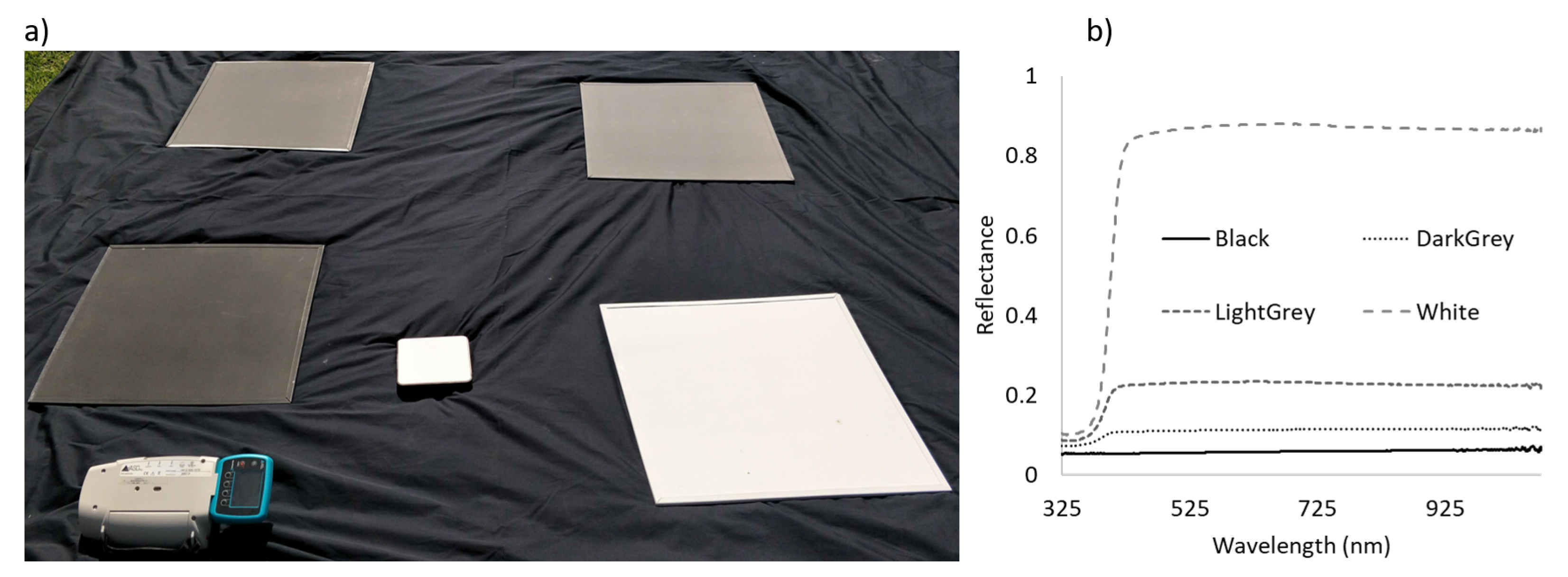
Four greyscaled spectral panels (white, light-grey, dark-grey and black) were developed using a combination of barium sulphate and white paint [51]. These panels were deployed during each flight for atmospheric correction and reflectance calibration purposes. The MicaSence calibration panel and DLS were not utilised for four reasons: (a) the user manual recommended that the sampling method of the calibration panel was not feasible for the heavy UAV used in this study [52]; (b) the DLS without a cosine corrector could have directional variation [53,54]; (c) the use of four greyscaled spectral panels instead of one allowed more control during the empirical line correction; and (d) capturing the reflectance data of both plants and spectral panels from the same altitude potentially better corrected the atmospheric effects.
2.3.2. Reference Ground Data Acquisition
The ground reference data included the in-field kc measurement using the Paso Panel. The Paso Panel measured the output current at full sun and when placed under the canopy. During the measurement, the panel was placed orthogonally to the cordon, approximately 10–15 from the ground. The final adjustment was made to make sure that the panel was level, that the vine shadow was approximately in the middle of the panel, and that no shadow was cast to the panel from the crew. For each vine, two under-vine measurements were made, one on each cordon. After measuring every four vines, the full sun measurement was repeated to accommodate for any changes in incident solar radiation. The kc was computed analytically using Equation (1) [40].
where is the length of the Paso Panel, is the row spacing, and are the current readings made under full sun and the canopy shade, respectively.
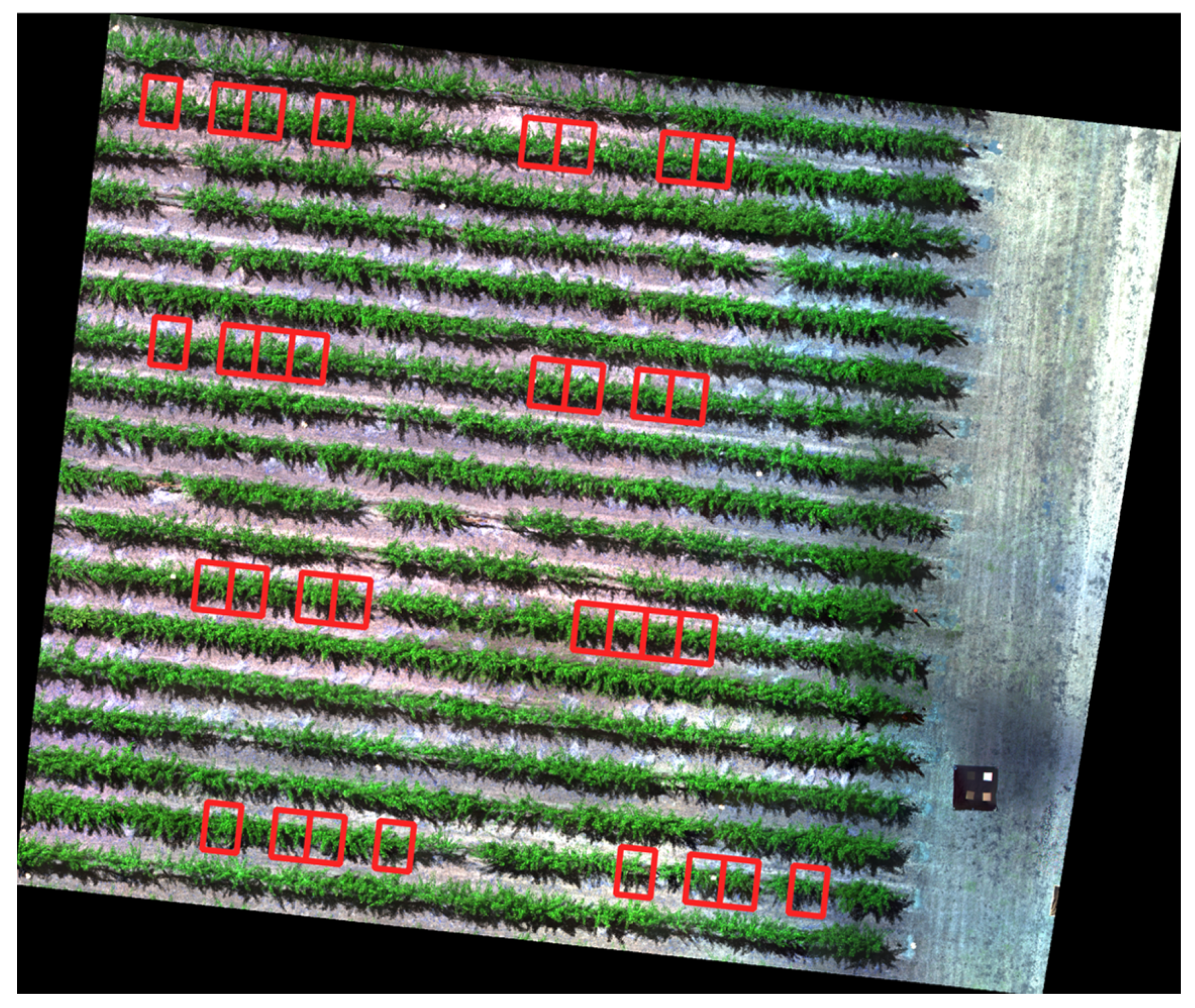
Thirty-two ground references were measured at both ends of the vineyard per timepoint (Figure 2). Note that this dataset is a part of a bigger irrigation trial. The irrigation trial tested several irrigation strategies using environmental, soil and plant-based sensors to schedule irrigation. The average seasonal irrigation for the block was approximately 0.5 ML ha for the vine density of 1700 vines ha. In the trial, the investigated irrigation strategies were limited to specific rows, resulting in the ground sampling vines for this kc study being limited to specific rows throughout the season. Lacking the spatial distribution presented a risk of ground-based kc values being clustered within a tight range. However, a wide range of kc values was observed due to the distribution of sampling timepoints (early-, mid- and late-season), multiple seasons, and the different irrigation treatment-induced physiological responses.
2.4. Data Processing
2.4.1. Extraction of Canopy Level Data
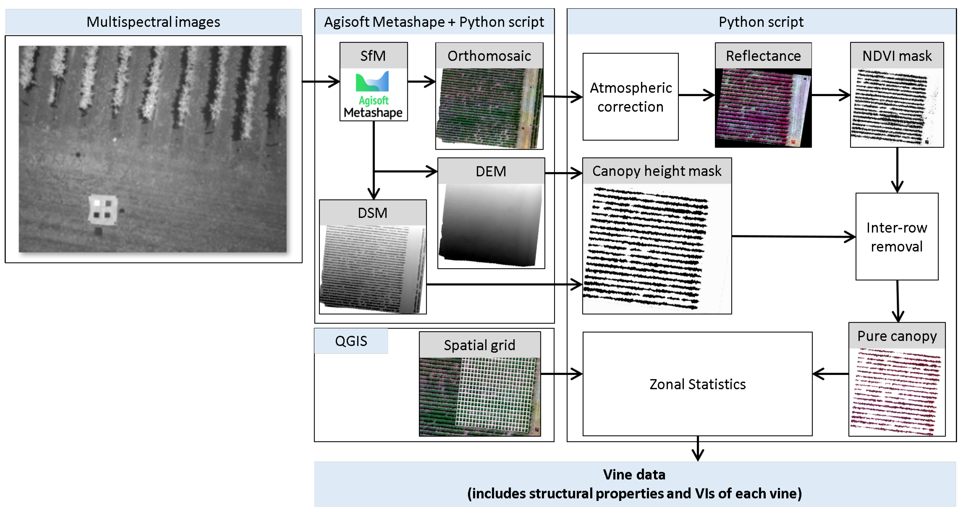
The multispectral images were mosaicked using standard SfM workflow in Agisoft Metashape (Agisoft LLC, St. Petersburg, Russia) Professional Version 1.6.2. The products generated using the software included the digital elevation model (DEM), the digital surface model (DSM) and the orthomosaic, all expressed in projected coordinate frame MGA zone 54 (EPSG:28354). The temporal orthomosaics were processed using a custom-developed Python script routine that performed the radiometric/atmospheric calibration, masking, and data extraction from all individual canopies.
The radiometric/atmospheric calibration of the temporal orthomosaics was performed with respect to the reflectance of the four greyscaled spectral panels that were deployed during each flight (Figure 3). Using the reflectance of the four panels at five bands, the orthomosaics were converted to the reflectance by empirical line correction [55,56]. As the four greyscaled panels were used regularly in the field condition, the panels could degrade due to repeated handling, hence the panels were also calibrated regularly. The four panels were calibrated twice each season at the start and at the end (e.g., before budburst and after harvest) using an ASD HandHeld 2 spectroradiometer (Malvern Panalytical Ltd., Malvern, UK) and a calibrated Spectralon. The HandHeld 2 acquired the spectral signature of the panels within the spectral range of 325–1075 with a spectral resolution of 3 . The sampled spectral profile of the four panels was resampled using a Gaussian model to match the wavelength centre and wavelength bandwidth of the RedEdge-MX sensor.
A canopy height mask and a normalised difference vegetation index (NDVI) mask were generated for each timepoint to mask out the non-canopy pixels including the inter-row, wooden post, and so forth. The canopy height mask was created by offsetting the DEM and DSM and applying a global threshold of 0.7 (average height of the canopies was 1.7 ). The NDVI mask was created by computing the NDVI and a global threshold of 0.3 (average NDVI of the canopies was 0.6). The combination of the two masks effectively removed the inter-row vegetation, background soil and wooden posts, as well as diseased vines with significantly smaller canopies. Using the macrostructure information of the vineyard (i.e., vine spacing and row spacing), a spatial grid was created using QGIS version 3.16.2 and was approximately aligned with the vines—effectively placing a single canopy within each polygon of the grid. Each polygon of the grid was separated with a buffer of 20 to limit the crossover of the canopy to the adjacent polygon. Using the buffered and aligned grid over the masked orthomosaic, pure canopy data were extracted from every single vine and written in the attribute table. The extracted data included the mean spectral reflectance as well as canopy pixel count and height. Using the total pixels within a canopy, various structural information was derived including canopy area (c_area), canopy width, and canopy fraction cover within the ground area per vine (row spacing × vine spacing). Using the reflectance of five bands, several spectral indices were computed. This structural information and the spectral indices were then exported as a CSV file (see Figure 4).
2.4.2. Spectral and Structural Feature Selection
This study incorporated numerous spectral features computed using the blue, green, red, rededge and near infrared bands (e.g., indices available at [57,58,59,60]), structural features (e.g., available at [44,61]) and canopy fraction cover [62], as well as a number of custom/adopted features (e.g., cummulative NDVI, canopy width, canopy area and canopy volume above cordon). A correlation analysis of each spectral and structural feature was performed with respect to the ground measured kc for all the timepoints combined. The features that revealed no significant (Pearson test, p-value > 0.05) correlation with kc were discarded for the modelling. Furthermore, the features with a high degree of collinearity (correlation coefficient > 0.95) were refined to select only one with the highest significance or correlation coefficient. These two steps of feature filtering eliminated most of the spectral/structural features that were initially computed for consideration. The features retained after the two elimination processes were taken as an input for developing kc prediction models (see Table 1).
2.4.3. Modelling
Within the five timepoints of the two seasons, a total of 320 datapoints were acquired, which included remotely sensed spectral/structural features and the corresponding ground-reference kc. Outliers in the dataset were investigated and removed using Cook’s distance (2/n), which reduced the number of datapoints to 231 [68,69]. The spectral/structural features synthesised in Table 1 were used to develop predictive models of kc. The training and testing datasets were split randomly in the ratio of 3:1 (173 training and 58 testing datapoints). Using the training dataset and the leave-one-out cross-validation, kc prediction models were developed. This leave-one-out approach of fit-control recursively develops a model and validates on one random datapoint until all the datapoints are used for validation [70]. Various models, such as the simple linear model (SLM), generalised linear model (GLM), generalised additive model (GAM), neural network model (NNM) and random forest model (RFM) were developed using the caret package in R programming languages (Version 4.0.4, RStudio Version 1.4.1106) [71,72,73]. The final refined model was tested on the testing dataset (58 datapoints). The model performance was evaluated using indicators including R squared (R2), Root Mean Square Error (RMSE) and mean absolute error (MAE).
3. Results
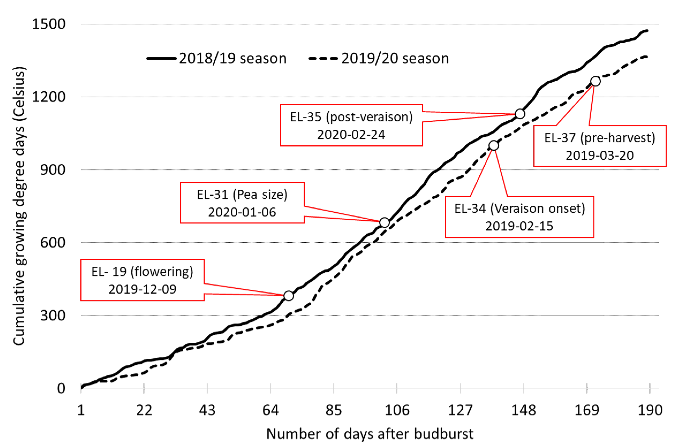
The grape growing season in the Coonawarra region starts relatively late with budburst in late October, reaching flowering approximately in December, pea-sized berries in January, véraison in February and harvest in April. The cumulative growing degree days for the two seasons are computed by integrating the local weather station data (Australian Government, Bureau of Meteorology, weather station number 026091, Coonawarra, SA, Australia) starting from the budbrust up to the grape harvest (see Figure 5). The field data acquisition timepoints (3 timepoints in the 2018/19 season and 2 timepoints in the 2019/20 season) and the corresponding phenological stage of the grapevine are shown in the figure. In comparison, the 2019/20 season was cooler with fewer heatwaves and less extreme temperatures.
The evolution of kc, along with the most significant spectral/structural features, are presented in Figure 6. The displayed features had the highest significance and correlation coefficient with kc. The seasonal kc values followed the pattern, which was noted physically and observed in the canopy LAI measurements, of rapid canopy growth until the véraison and stability after that. The kc started at a mean value of 0.48 at the start of the season and steadily increased to a mean value of 0.67 by the end of the season. The trends of NDVI and ENDVI2 appear to be less sensitive to canopy growth, while the c_area was the most sensitive, particularly in the early season between fruit set and pea-sized berries. Between the pea size and véraison, all of the remote sensing temporal trends do not appear to reflect the kc trend. Post véraison, all the indices show a strong agreement with each other and reflect little to no changes in canopy development/growth. The decrease in spectral indices post véraison may be reflecting the depletion of nitrogen in the vine, including the leaves [74,75]. The seasonal evolution graph suggests that either the c_area alone or a combination of c_area and spectral features could be the best predictors of kc at any timepoint. The best performing model for each timepoint could incorporate the timepoint specific data. However, this study assesses a holistic model to reduce the timepoint specific bias due to the small sample size, as well as to provide a robust predictor that is not limited by the growth stage of the plant.
Among various spectral indices and structural parameters (not listed exclusively here), few of the features were selected for modelling purposes following the removal of non-significant as well as collinear features. The correlogram in Figure 7 shows the selected indices, their statistical significance and correlation coefficients with the response variable, kc. The c_area had the strongest correlation with kc (highly significant and highest correlation coefficient). Composite feature cumulative NDVI and spectral features NDVI ENDVI2 were the second-tier features showing a strong correlation with kc, while other features, such as the greenness index (GI), ENDVI3, visible-band difference vegetation index (VDVI) and plant height (p_height), had a weak but significant correlation.
To develop kc models, the dataset (231 datapoints) was split into training and testing on a ratio of 3:1. The training dataset was used to train the model while the testing dataset was used to access the performance accuracy. The leave-one-out cross-validation approach ensured that a large number of datapoints (172) were available for each of the model generations. The best univariate indicator of kc was the c_area, which performed with reasonable accuracy (R2 = 0.295, RMSE = 0.091, MAE = 0.076). Multidimensional regression using all the features substantially improved the prediction accuracy (e.g., GLM) with improved AIC (SLM AIC: −340.0, GLM AIC: −411.7). Further improvement in the prediction was achieved using non-linear-multidimensional models (e.g., GAM with AIC of −461.7) and machine learning models such as CNN (a 8-5-1 network with 51 weights) and RFM (ntree = 500, mtry = 3). While all the multidimensional models investigated used the same input features (listed in Table 1, the features that ended up being important in all the models were significantly different. For example, the RFM, which performed the best, had c_area as the most important feature whereas the CNN, which used cum_NDVI, performed relatively poorly. In addition to the leave-one-out, a k-fold cross-validation approach was tested, which resulted in a similar trend in the model accuracy—RFM performing the best of all the models evaluated in this study (see Table 2).
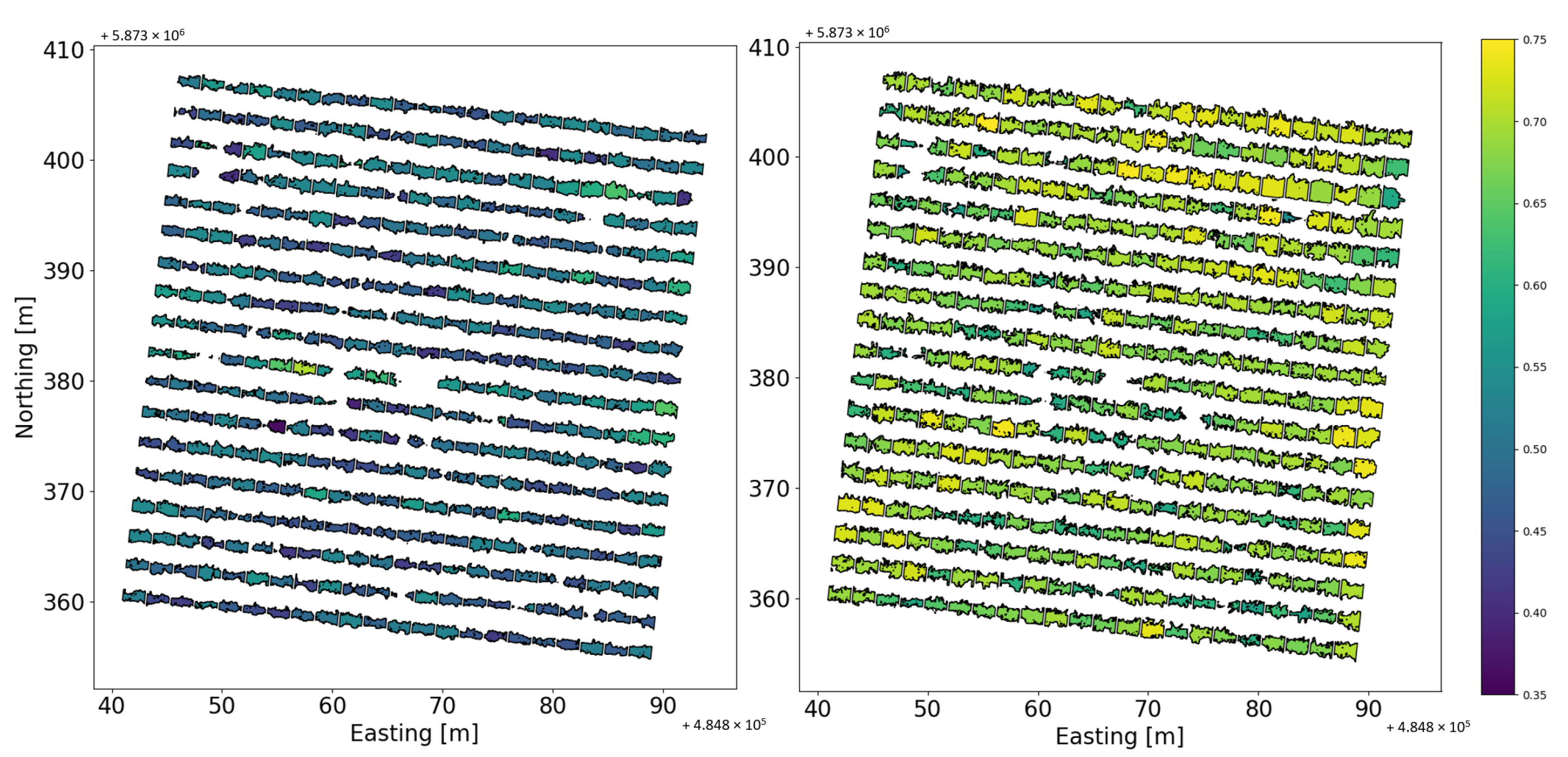
The simple linear model provided the most straightforward model while the RFM provided the most accurate model for estimating kc. The RFM model was used to further predict spatial kc values at the vineyard scale at two key phenological stages of the vine (Figure 8). Using the estimated kc values, along with the weather data (temperature, humidity, wind speed), the spatial irrigation requirements of the vineyard were computed on a per vine basis.
4. Discussion
There exist differences in mesoclimate between different sites and within the site receiving uniform irrigation. For instance, the two sites used in this study received uniform irrigation despite highly variable soil depth. This variability presents a significant challenge for irrigation management that could be partly overcome by adopting high-resolution data capture. A significant advantage of UAV remote sensing in precision irrigation is the unprecedented spatial details that can reveal spatial variability within a vineyard receiving uniform irrigation. This detailed (canopy-specific) level of information is, however, not fully exploitable, that is, canopy-specific irrigation management is not practicable. The current irrigation management technology in vineyards generally has a fixed infrastructure, which makes the spatial control of the irrigation unfeasible or costly to incorporate. A potential benefit could lie in the improvement of the zoning of the vineyards such that zones receiving uniform irrigation have reduced spatial variability [76]. Using spatial clustering, irrigation zones can be set to minimise spatial variability whilst still maintaining economic viability [77].
The kc is an evolving parameter that changes together with the development stage of the crop, canopy cover and architecture, and transpiration [10,40]. As such, different crops with different management practices will have a unique evolution of water requirements and kc values throughout the various phenological stages [31,43,78]. Even for a single crop, such as a grapevine, a single kc value may lead to over- or under-irrigation depending on the time of the year. This has numerous implications for management. The availability of a time series of kc maps will allow spatially explicit parameterisation of models for irrigation management and this will facilitate improved realism in models (see [7] for a recent review of models). Spatio-temporal estimates of kc will help with implementing regulated deficit irrigation (RDI). A typical RDI regime necessitates a minimum of two timepoints of kc values. The temporal evolution of kc seems to follow the thermal time (GDD) graph; however, it requires further temporally-intensive data at multiple seasons for verification. Such co-evolution of kc and GDD, if established, could require only a few timepoints of kc determination that can be extrapolated temporally based on the evolution of the thermal GDD.
This research could have limitations due to the study of just two seasons of data and the lack of spatial distribution of ground reference. Two seasons of data were considered sufficient as the investigated vines were mature and were managed using set management practices, which resulted in minimal seasonality effect on the canopy structure and architecture. However, there could still be some underlying seasonal variability requiring further data acquisition. The spatial distribution of the ground reference was set by a larger irrigation treatment study, which this research was a part of. The ground reference measurement vines were selected based on the physiology of the plant from set rows to minimise the inter-vine variability and to construct the irrigation system. As a result, only the selected vines that were located in certain rows were measured. However, despite this lack of spatial distribution, our dataset captured a wide extent of kc measurement values, predominantly due to the data acquisition at early-, mid-, and late-season, as well as due to the application of various irrigation treatments. Moreover, the UAV-estimated range of kc values was equivalent to the ground-observed range of kc values.
The kc is generally measured on the ground from several representative samples within each irrigation zone. This approach, however, does not capture the entire variability within a field and the selection of samples can be subjective to the user. UAV-based observation of the entire irrigation zone could provide a more unbiased and holistic view of the vineyard. Moreover, the UAV-based kc estimation incorporates measurements from the entire canopy while the kc measured on the ground using the Paso Panel incorporates a section of the canopy. For instance, we sampled kc values once from each side of the cordon. This sampling strategy is equivalent to the incorporation of 0.6 out of 2.1 of the canopy cordon. As a result, the ground sampling is computed by observing less than 30% of the canopy foliage while the aerial sampling incorporates the entire canopy foliage. Hence, some errors associated with the UAV-based modelling of kc could also be attributed to the Paso Panel acquired ground data. The UAV-based kc values could, therefore, be more robust than is expressed in the model performance results (Table 2).
Preliminary economic calculations based on Australian standards, and excluding the Research and Development cost, revealed that the UAV-based approach could be profitable for the industry in the long run. Measuring on a small scale (e.g., 1 vineyard), the Paso Panel approach costs approximately AU$20/vine/season considering the measurement of 50 vines from the 1 at six timepoints throughout the season. The UAV-based approach costs approximately AU$5/vine/season considering the initial capital investment and the measurement of 2000 vines from 1 at six timepoints. When considering a larger vineyard, for example, 20 , the UAV-based approach was substantially cheaper (AU$0.45/vine/season) while the Paso Panel approach cost remained approximately the same. The total cost of the UAV-based approach was substantially high in the first year; however, it becomes progressively cheaper on a per-vine-per-season basis. In subsequent years, both the UAV and Paso Panel approaches had approximately similar year-on-year running costs. Hence, following the initial capital investment in the UAV and multispectral camera, the industry will be able to measure every vine by spending a similar amount as on the Paso Panel based approach. However, a detailed cost–benefit analysis in this regard is needed to establish a complete understanding of the costs associated with the adaptation of this technology and its benefits, both short- and long-term.
For non-horticultural homogenous field crops, the satellite-based estimation of kc is very reliable [30,31,38]. Complexity in the horticultural setting specifically due to inter-row bare/vegetated areas reduces the estimation accuracies. In vineyards, R2 of 0.177 and 0.426 was achieved using satellite-based SAR and NDVI images, respectively [79]. In a ground-based study of a vineyard, [43] showed a linear relationship between the ground-based LAI and the ground-based kc in Cabernet Sauvignon with an R2 of 0.66. In a similar study, [40] estimated the kc of the Thompson Seedless table grape as a function of leaf area per vine (R2 = 0.87), LAI (R2 = 0.87) and shaded area (R2 = 0.95). The higher estimation accuracy with the table grape canopies can be attributed to the overhead trellis systems as compared to the VSP trellis with the wine grapes [43]. Our study of kc on sprawling Cabernet Sauvignon wine grapes is comparable to the ground-based study presented in [43]. Using UAV remote sensing, our study presented the capability of remotely measuring kc with a similar accuracy to that of the ground-based measurements (R2 = 0.675). This capability combined with the benefits of remote sensing in terms of efficiently and inexpensively sampling a much larger area (several hectares) could increase the use of UAV in lieu of field sampling.
The kc in vineyards is highly variable and can be influenced by vine management practices, soil depth, rooting systems and vine training systems, among other factors. While there are kc maps freely accessible to growers, these maps will require a site-, region-, and crop-specific ground calibration to establish their usability [30,33]. Using a UAV-based approach, the most practical solution from a grower’s perspective could be with the use of a simple RGB camera on an autonomous UAV to compute the c_area as a proxy of kc. Using just the c_area as an input, kc was estimated, in this study, with an R2 of 0.295, an RMSE of 0.091, and an MAE of 0.076. Given the improved level of autonomy of the UAVs and the increased efficiencies via data processing pipelines, estimating irrigation requirements at multiple timepoints of the season could be within reach for growers using a UAV-based RGB camera. This will improve the precision of the irrigation by computing spatially explicit irrigation requirements for each vine as well as for the entire irrigation zone. However, for the most accurate quantitative estimation, growers could consider sophisticated models such as GLM, GAM or machine learning.
5. Conclusions
In this article, we demonstrated the application of an unmanned aircraft system to estimating the crop coefficient and subsequent irrigation requirements of vineyards. The spectral indices were highly correlated to kc until the véraison timepoint. After véraison, the correlation between the spectral indices and kc value started to diverge. The structural features presented the highest correlation coefficient and statistical significance with kc values throughout the season. Combining both the spectral reflectance and structural features of the grapevine provided a robust estimation of kc for both early as well as late in the season. Incorporating kc values with an energy balance model can provide an estimate of the irrigation requirements at different phenological stages. Preliminary economic analysis revealed that the proposed UAV-based method was the most cost effective and quickest method for estimating the kc and subsequent crop water needs per vine. With the continued development of UAV and battery technology, we envision the increased use of UAV remote sensing for the estimation of irrigation requirements in both small and large vineyards. Future research directions could include irrigation thresholding and automated triggering based on the measured crop water needs and the monitoring of vines and their physiology. While ETc provided a basis for evidence-based irrigation, more precise control of grapevine irrigation needs could require the use of plant-based sensors such as microtensiometers. A combination of both ET- and plant-based sensors could be a way forward to potentially maximise water use efficiency on a fine to a large scale.
Author Contributions
All authors conceived the initial design of the research. D.G. acquired the remote sensing and together with V.P. the ground data. D.G. processed/analysed the data and together with V.P. interpreted the results. D.G. prepared the manuscript. All authors contributed to the review of the manuscript. All authors have read and agreed to the published version of the manuscript.
Funding
This research was funded by Wine Australia (Grant number: UA 1803-1.3) bilateral project.
Acknowledgments
The authors would like to acknowledge Rochelle Schlank, Antoine Lespes, Caitlin Griffiths, Catherine Kidman, and Courtney Handford for their assistance in the field data collection at different stages; the Wynns Coonawarra Estate for providing test site for this study; the funding body Wine Australia; The University of Adelaide; and the anonymous reviewers for their contribution.
Conflicts of Interest
The authors declare no conflict of interest.
References
- Ummenhofer, C.C.; England, M.H.; McIntosh, P.C.; Meyers, G.A.; Pook, M.J.; Risbey, J.S.; Gupta, A.S.; Taschetto, A.S. What causes southeast Australia’s worst droughts? Geophys. Res. Lett. 2009, 36. [Google Scholar] [CrossRef] [Green Version]
- King, A.D.; Pitman, A.J.; Henley, B.J.; Ukkola, A.M.; Brown, J.R. The role of climate variability in Australian drought. Nat. Clim. Chang. 2020, 10, 177–179. [Google Scholar] [CrossRef]
- Paydar, Z.; Qureshi, M. Irrigation water management in uncertain conditions—Application of Modern Portfolio Theory. Agric. Water Manag. 2012, 115, 47–54. [Google Scholar] [CrossRef]
- Smith, R. Review of Precision Irrigation Technologies and Their Applications; Technical Report; University of Southern Queensland: Toowoomba, Australia, 2011. [Google Scholar]
- Mulla, D.J. Twenty five years of remote sensing in precision agriculture: Key advances and remaining knowledge gaps. Biosyst. Eng. 2013, 114, 358–371. [Google Scholar] [CrossRef]
- Gautam, D.; Pagay, V. A Review of Current and Potential Applications of Remote Sensing to Study the Water Status of Horticultural Crops. Agronomy 2020, 10, 140. [Google Scholar] [CrossRef] [Green Version]
- Knowling, M.; Bennett, B.; Ostendorf, B.; Westra, S.; Walker, R.; Pellegrino, A.; Edwards, E.; Collins, C.; Pagay, V.; Grigg, D. Bridging the gap between data and decisions in viticulture: A review of process-based models. Agric. Syst. 2021, 193. [Google Scholar] [CrossRef]
- Fereres, E.; Soriano, M.A. Deficit irrigation for reducing agricultural water use. J. Exp. Bot. 2007, 58, 147–159. [Google Scholar] [CrossRef] [Green Version]
- Iniesta, F.; Testi, L.; Orgaz, F.; Villalobos, F. The effects of regulated and continuous deficit irrigation on the water use, growth and yield of olive trees. Eur. J. Agron. 2009, 30, 258–265. [Google Scholar] [CrossRef]
- Allen, R.G.; Pereira, L.S.; Raes, D.; Smith, M. Crop evapotranspiration-Guidelines for computing crop water requirements-FAO Irrigation and drainage paper 56. Fao Rome 1998, 300, D05109. [Google Scholar]
- Hoffmann, H.; Nieto, H.; Jensen, R.; Guzinski, R.; Zarco-Tejada, P.; Friborg, T. Estimating evaporation with thermal UAV data and two-source energy balance models. Hydrol. Earth Syst. Sci. 2016, 20, 697–713. [Google Scholar] [CrossRef] [Green Version]
- Nieto, H.; Bellvert, J.; Kustas, W.P.; Alfieri, J.G.; Gao, F.; Prueger, J.; Torres-Rua, A.; Hipps, L.E.; Elarab, M.; Song, L. Unmanned airborne thermal and mutilspectral imagery for estimating evapotranspiration in irrigated vineyards. In Proceedings of the 2017 IEEE International Geoscience and Remote Sensing Symposium (IGARSS), Fort Worth, TX, USA, 23–28 July 2017; pp. 5510–5513. [Google Scholar]
- Niu, H.; Hollenbeck, D.; Zhao, T.; Wang, D.; Chen, Y. Evapotranspiration Estimation with Small UAVs in Precision Agriculture. Sensors 2020, 20, 6427. [Google Scholar] [CrossRef]
- Niu, H.; Wang, D.; Chen, Y. Estimating actual crop evapotranspiration using deep stochastic configuration networks model and UAV-based crop coefficients in a pomegranate orchard. In Autonomous Air and Ground Sensing Systems for Agricultural Optimization and Phenotyping V; International Society for Optics and Photonics: San Diego, CA, USA, 2020; Volume 11414, p. 114140C. [Google Scholar]
- Bellvert, J.; Adeline, K.; Baram, S.; Pierce, L.; Sanden, B.L.; Smart, D.R. Monitoring crop evapotranspiration and crop coefficients over an almond and pistachio orchard throughout remote sensing. Remote Sens. 2018, 10, 2001. [Google Scholar] [CrossRef] [Green Version]
- Bellvert, J.; Zarco-Tejada, P.; Gonzalez-Dugo, V.; Girona, J.; Fereres, E. Scheduling vineyard irrigation based on mapping leaf water potential from airborne thermal imagery. In Precision Agriculture’13; Springer: Berlin/Heidelberg, Germany, 2013; pp. 699–704. [Google Scholar]
- Bellvert, J.; Girona, J. The use of multispectral and thermal images as a tool for irrigation scheduling in vineyards. Use Remote. Sens. Geogr. Inf. Syst. Irrig. Manag. Southwest Eur. 2012, 67, 131–137. [Google Scholar]
- Bellvert, J.; Zarco-Tejada, P.J.; Marsal, J.; Girona, J.; González-Dugo, V.; Fereres, E. Vineyard irrigation scheduling based on airborne thermal imagery and water potential thresholds. Aust. J. Grape Wine Res. 2016, 22, 307–315. [Google Scholar] [CrossRef] [Green Version]
- Gonzalez-Dugo, V.; Goldhamer, D.; Zarco-Tejada, P.J.; Fereres, E. Improving the precision of irrigation in a pistachio farm using an unmanned airborne thermal system. Irrig. Sci. 2015, 33, 43–52. [Google Scholar] [CrossRef]
- López-Urrea, R.; Montoro, A.; Mañas, F.; López-Fuster, P.; Fereres, E. Evapotranspiration and crop coefficients from lysimeter measurements of mature ‘Tempranillo’wine grapes. Agric. Water Manag. 2012, 112, 13–20. [Google Scholar] [CrossRef]
- Williams, L.; Phene, C.; Grimes, D.; Trout, T. Water use of mature Thompson Seedless grapevines in California. Irrig. Sci. 2003, 22, 11–18. [Google Scholar] [CrossRef]
- Li, Z.L.; Tang, R.; Wan, Z.; Bi, Y.; Zhou, C.; Tang, B.; Yan, G.; Zhang, X. A review of current methodologies for regional evapotranspiration estimation from remotely sensed data. Sensors 2009, 9, 3801–3853. [Google Scholar] [CrossRef] [Green Version]
- Liou, Y.A.; Kar, S.K. Evapotranspiration estimation with remote sensing and various surface energy balance algorithms—A review. Energies 2014, 7, 2821–2849. [Google Scholar] [CrossRef] [Green Version]
- Zhang, K.; Kimball, J.S.; Running, S.W. A review of remote sensing based actual evapotranspiration estimation. Wiley Interdiscip. Rev. Water 2016, 3, 834–853. [Google Scholar] [CrossRef]
- Kullberg, E.G.; DeJonge, K.C.; Chávez, J.L. Evaluation of thermal remote sensing indices to estimate crop evapotranspiration coefficients. Agric. Water Manag. 2017, 179, 64–73. [Google Scholar] [CrossRef] [Green Version]
- Ihuoma, S.O.; Madramootoo, C.A. Recent advances in crop water stress detection. Comput. Electron. Agric. 2017, 141, 267–275. [Google Scholar] [CrossRef]
- Tang, J.; Han, W.; Zhang, L. UAV Multispectral Imagery Combined with the FAO-56 Dual Approach for Maize Evapotranspiration Mapping in the North China Plain. Remote Sens. 2019, 11, 2519. [Google Scholar] [CrossRef] [Green Version]
- Poblete-Echeverría, C.; Ortega-Farias, S. Evaluation of single and dual crop coefficients over a drip-irrigated M erlot vineyard (Vitis vinifera L.) using combined measurements of sap flow sensors and an eddy covariance system. Aust. J. Grape Wine Res. 2013, 19, 249–260. [Google Scholar] [CrossRef]
- Cancela, J.; Fandiño, M.; Rey, B.; Martínez, E. Automatic irrigation system based on dual crop coefficient, soil and plant water status for Vitis vinifera (cv Godello and cv Mencía). Agric. Water Manag. 2015, 151, 52–63. [Google Scholar] [CrossRef]
- Kamble, B.; Kilic, A.; Hubbard, K. Estimating crop coefficients using remote sensing-based vegetation index. Remote Sens. 2013, 5, 1588–1602. [Google Scholar] [CrossRef] [Green Version]
- Zhang, H.; Anderson, R.G.; Wang, D. Satellite-based crop coefficient and regional water use estimates for Hawaiian sugarcane. Field Crops Res. 2015, 180, 143–154. [Google Scholar] [CrossRef] [Green Version]
- Ramírez-Cuesta, J.M.; Mirás-Avalos, J.M.; Rubio-Asensio, J.S.; Intrigliolo, D.S. A novel ArcGIS toolbox for estimating crop water demands by integrating the dual crop coefficient approach with multi-satellite imagery. Water 2019, 11, 38. [Google Scholar] [CrossRef] [Green Version]
- Montgomery, J.; Hornbuckle, J.; Hume, I.; Vleeshouwer, J. IrriSAT—Weather based scheduling and benchmarking technology. In Proceedings of the 17th ASA Conference, Hobart, Australia, 20–24 September 2015; pp. 20–24. [Google Scholar]
- Trout, T.; Johnson, L. Estimating crop water use from remotely sensed NDVI, crop models, and reference ET. In Proceedings of the USCID Fourth International Conference on Irrigation and Drainage, Role of Irrigation and Drainage in a Sustainable Future, Sacramento, CA, USA, 3–6 October 2007; pp. 3–6. [Google Scholar]
- Sanchez, L.; Sams, B.; Alsina, M.; Hinds, N.; Klein, L.; Dokoozlian, N. Improving vineyard water use efficiency and yield with variable rate irrigation in California. Adv. Anim. Biosci. 2017, 8, 574–577. [Google Scholar] [CrossRef]
- Er-Raki, S.; Rodriguez, J.; Garatuza-Payan, J.; Watts, C.; Chehbouni, A. Determination of crop evapotranspiration of table grapes in a semi-arid region of Northwest Mexico using multi-spectral vegetation index. Agric. Water Manag. 2013, 122, 12–19. [Google Scholar] [CrossRef]
- Choudhury, B.J.; Ahmed, N.U.; Idso, S.B.; Reginato, R.J.; Daughtry, C.S. Relations between evaporation coefficients and vegetation indices studied by model simulations. Remote Sens. Environ. 1994, 50, 1–17. [Google Scholar] [CrossRef]
- Hunsaker, D.J.; Pinter, P.J.; Kimball, B.A. Wheat basal crop coefficients determined by normalized difference vegetation index. Irrig. Sci. 2005, 24, 1–14. [Google Scholar] [CrossRef]
- Samani, Z.; Bawazir, A.S.; Bleiweiss, M.; Skaggs, R.; Longworth, J.; Tran, V.D.; Pinon, A. Using remote sensing to evaluate the spatial variability of evapotranspiration and crop coefficient in the lower Rio Grande Valley, New Mexico. Irrig. Sci. 2009, 28, 93. [Google Scholar] [CrossRef] [Green Version]
- Williams, L.; Ayars, J. Grapevine water use and the crop coefficient are linear functions of the shaded area measured beneath the canopy. Agric. For. Meteorol. 2005, 132, 201–211. [Google Scholar] [CrossRef]
- Picón-Toro, J.; González-Dugo, V.; Uriarte, D.; Mancha, L.; Testi, L. Effects of canopy size and water stress over the crop coefficient of a “Tempranillo” vineyard in south-western Spain. Irrig. Sci. 2012, 30, 419–432. [Google Scholar] [CrossRef] [Green Version]
- Santos, L.; Ferraz, G.; Diotto, A.; Barbosa, B.; Maciel, D.; Andrade, M.; Ferraz, P.; Rossi, G. Coffee crop coefficient prediction as a function of biophysical variables identified from RGB UAS images. Agron. Res. 2020, 18, 1463–1471. [Google Scholar]
- Munitz, S.; Schwartz, A.; Netzer, Y. Water consumption, crop coefficient and leaf area relations of a Vitis vinifera cv. ’Cabernet Sauvignon’ vineyard. Agric. Water Manag. 2019, 219, 86–94. [Google Scholar] [CrossRef]
- Matese, A.; Di Gennaro, S.F.; Berton, A. Assessment of a canopy height model (CHM) in a vineyard using UAV-based multispectral imaging. Int. J. Remote Sens. 2017, 38, 2150–2160. [Google Scholar] [CrossRef]
- Jurado, J.M.; Ortega, L.; Cubillas, J.J.; Feito, F. Multispectral mapping on 3D models and multi-temporal monitoring for individual characterization of olive trees. Remote Sens. 2020, 12, 1106. [Google Scholar] [CrossRef] [Green Version]
- Banks, G.; Sharpe, S. Wine, regions and the geographic imperative: The Coonawarra example. N. Z. Geogr. 2006, 62, 173–184. [Google Scholar] [CrossRef]
- Mee, A.C.; Bestland, E.A.; Spooner, N.A. Age and origin of Terra Rossa soils in the Coonawarra area of South Australia. Geomorphology 2004, 58, 1–25. [Google Scholar] [CrossRef]
- Coombe, B.G. Growth stages of the grapevine: Adoption of a system for identifying grapevine growth stages. Aust. J. Grape Wine Res. 1995, 1, 104–110. [Google Scholar] [CrossRef]
- Mlambo, R.; Woodhouse, I.H.; Gerard, F.; Anderson, K. Structure from motion (SfM) photogrammetry with drone data: A low cost method for monitoring greenhouse gas emissions from forests in developing countries. Forests 2017, 8, 68. [Google Scholar] [CrossRef] [Green Version]
- Dandois, J.P.; Olano, M.; Ellis, E.C. Optimal altitude, overlap, and weather conditions for computer vision UAV estimates of forest structure. Remote Sens. 2015, 7, 13895–13920. [Google Scholar] [CrossRef] [Green Version]
- Sanches, I.; Tuohy, M.; Hedley, M.; Bretherton, M. Large, durable and low-cost reflectance standard for field remote sensing applications. Int. J. Remote Sens. 2009, 30, 2309–2319. [Google Scholar] [CrossRef]
- RedEdge, M. Multispectral Camera User Manual; MicaSense Inc.: Seattle, WA, USA, 2015; p. 33. [Google Scholar]
- Tu, Y.H.; Phinn, S.; Johansen, K.; Robson, A. Assessing radiometric correction approaches for multi-spectral UAS imagery for horticultural applications. Remote Sens. 2018, 10, 1684. [Google Scholar] [CrossRef] [Green Version]
- Bendig, J.; Gautam, D.; Malenovskỳ, Z.; Lucieer, A. Influence of cosine corrector and UAS platform dynamics on airborne spectral irradiance measurements. In Proceedings of the IGARSS 2018-2018 IEEE International Geoscience and Remote Sensing Symposium, Valencia, Spain, 22–27 July 2018; pp. 8822–8825. [Google Scholar]
- Smith, G.M.; Milton, E.J. The use of the empirical line method to calibrate remotely sensed data to reflectance. Int. J. Remote Sens. 1999, 20, 2653–2662. [Google Scholar] [CrossRef]
- Wang, C.; Myint, S.W. A simplified empirical line method of radiometric calibration for small unmanned aircraft systems-based remote sensing. IEEE J. Sel. Top. Appl. Earth Obs. Remote Sens. 2015, 8, 1876–1885. [Google Scholar] [CrossRef]
- Baluja, J.; Diago, M.P.; Balda, P.; Zorer, R.; Meggio, F.; Morales, F.; Tardaguila, J. Assessment of vineyard water status variability by thermal and multispectral imagery using an unmanned aerial vehicle (UAV). Irrig. Sci. 2012, 30, 511–522. [Google Scholar] [CrossRef]
- Zarco-Tejada, P.J.; Berjón, A.; López-Lozano, R.; Miller, J.R.; Martín, P.; Cachorro, V.; González, M.; De Frutos, A. Assessing vineyard condition with hyperspectral indices: Leaf and canopy reflectance simulation in a row-structured discontinuous canopy. Remote Sens. Environ. 2005, 99, 271–287. [Google Scholar] [CrossRef]
- Zarco-Tejada, P.J.; Ustin, S.; Whiting, M. Temporal and spatial relationships between within-field yield variability in cotton and high-spatial hyperspectral remote sensing imagery. Agron. J. 2005, 97, 641–653. [Google Scholar] [CrossRef] [Green Version]
- Bannari, A.; Morin, D.; Bonn, F.; Huete, A. A review of vegetation indices. Remote Sens. Rev. 1995, 13, 95–120. [Google Scholar] [CrossRef]
- Bendig, J.; Yu, K.; Aasen, H.; Bolten, A.; Bennertz, S.; Broscheit, J.; Gnyp, M.L.; Bareth, G. Combining UAV-based plant height from crop surface models, visible, and near infrared vegetation indices for biomass monitoring in barley. Int. J. Appl. Earth Obs. Geoinf. 2015, 39, 79–87. [Google Scholar] [CrossRef]
- Pereira, L.; Paredes, P.; Melton, F.; Johnson, L.; Wang, T.; López-Urrea, R.; Cancela, J.; Allen, R. Prediction of crop coefficients from fraction of ground cover and height. Background and validation using ground and remote sensing data. Agric. Water Manag. 2020, 241, 106197. [Google Scholar] [CrossRef]
- Rouse, J.W.; Haas, R.H.; Schell, J.A.; Deering, D.W.; Harlan, J.C. Monitoring the Vernal Advancement and Retrogradation (Green Wave Effect) of Natural Vegetation; NASA/GSFC Type III Final Report; NASA/GSFC: Greenbelt, MD, USA, 1974; Volume 371. [Google Scholar]
- Tan, Y.; Wang, S.; Xu, B.; Zhang, J. An improved progressive morphological filter for UAV-based photogrammetric point clouds in river bank monitoring. ISPRS J. Photogramm. Remote Sens. 2018, 146, 421–429. [Google Scholar] [CrossRef]
- Xiaoqin, W.; Miaomiao, W.; Shaoqiang, W.; Yundong, W. Extraction of vegetation information from visible unmanned aerial vehicle images. Trans. Chin. Soc. Agric. Eng. 2015, 31, 152–159. [Google Scholar]
- Strong, C.J.; Burnside, N.G.; Llewellyn, D. The potential of small-Unmanned Aircraft Systems for the rapid detection of threatened unimproved grassland communities using an Enhanced Normalized Difference Vegetation Index. PLoS ONE 2017, 12, e0186193. [Google Scholar] [CrossRef] [PubMed] [Green Version]
- Susantoro, T.M.; Wikantika, K.; Saepuloh, A.; Harsolumakso, A.H. Selection of vegetation indices for mapping the sugarcane condition around the oil and gas field of North West Java Basin, Indonesia. IOP Conf. Ser. Earth Environ. Sci. 2018, 149, 012001. [Google Scholar] [CrossRef] [Green Version]
- Cook, R.D. Detection of influential observation in linear regression. Technometrics 1977, 19, 15–18. [Google Scholar]
- Walfish, S. A review of statistical outlier methods. Pharm. Technol. 2006, 30, 82. [Google Scholar]
- Vehtari, A.; Gelman, A.; Gabry, J. Practical Bayesian model evaluation using leave-one-out cross-validation and WAIC. Stat. Comput. 2017, 27, 1413–1432. [Google Scholar] [CrossRef] [Green Version]
- Kuhn, M. The Caret Package. Available online: https://cran.r-project.org/web/packages/caret/index.html (accessed on 5 July 2020).
- Kuhn, M. Building predictive models in R using the caret package. J. Stat. Softw. 2008, 28, 1–26. [Google Scholar] [CrossRef] [Green Version]
- Bivand, R. Implementing spatial data analysis software tools in R. Geogr. Anal. 2006, 38, 23–40. [Google Scholar] [CrossRef]
- Keller, M.; Hrazdina, G. Interaction of nitrogen availability during bloom and light intensity during veraison. II. Effects on anthocyanin and phenolic development during grape ripening. Am. J. Enol. Vitic. 1998, 49, 341–349. [Google Scholar]
- BELL, S.J.; Henschke, P.A. Implications of nitrogen nutrition for grapes, fermentation and wine. Aust. J. Grape Wine Res. 2005, 11, 242–295. [Google Scholar] [CrossRef]
- Bellvert, J.; Marsal, J.; Mata, M.; Girona, J. Identifying irrigation zones across a 7.5-ha ‘Pinot noir’vineyard based on the variability of vine water status and multispectral images. Irrig. Sci. 2012, 30, 499–509. [Google Scholar] [CrossRef]
- Ohana-Levi, N.; Bahat, I.; Peeters, A.; Shtein, A.; Netzer, Y.; Cohen, Y.; Ben-Gal, A. A weighted multivariate spatial clustering model to determine irrigation management zones. Comput. Electron. Agric. 2019, 162, 719–731. [Google Scholar] [CrossRef]
- Davis, S.; Dukes, M. Irrigation scheduling performance by evapotranspiration-based controllers. Agric. Water Manag. 2010, 98, 19–28. [Google Scholar] [CrossRef]
- Beeri, O.; Netzer, Y.; Munitz, S.; Mintz, D.F.; Pelta, R.; Shilo, T.; Horesh, A.; Mey-tal, S. Kc and LAI Estimations Using Optical and SAR Remote Sensing Imagery for Vineyards Plots. Remote Sens. 2020, 12, 3478. [Google Scholar] [CrossRef]
Figure 1.
Two Cabernet Sauvignon vineyards at the Wynns Coonawarra Estate, Coonawarra, SA, Australia used in this study of crop coefficient and irrigation requirements.
Figure 1.
Two Cabernet Sauvignon vineyards at the Wynns Coonawarra Estate, Coonawarra, SA, Australia used in this study of crop coefficient and irrigation requirements.
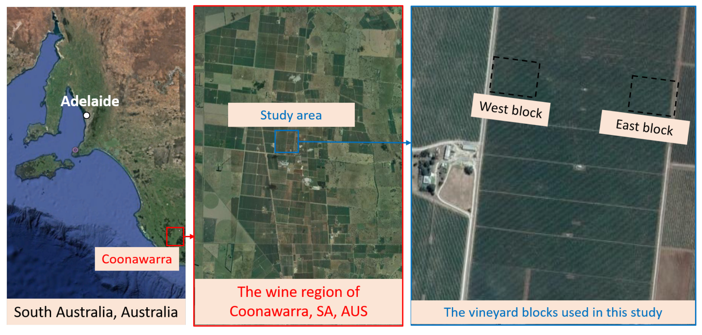
Figure 2.
The ground data are sampled from 64 vines (32 on the east and 32 on the west end) of the vineyard (east end shown) per timepoint (EL-31 shown). Highlighted are the measurement vines that were measured throughout the two seasons.
Figure 2.
The ground data are sampled from 64 vines (32 on the east and 32 on the west end) of the vineyard (east end shown) per timepoint (EL-31 shown). Highlighted are the measurement vines that were measured throughout the two seasons.

Figure 3.
The four greyscaled spectral panels (a) were calibrated twice each season—before the start and after the end of the season. The reflectance curve (b) shows the sample reflectance of the four panels acquired using the ASD handheld spectroradiometer and the calibrated spectralon.
Figure 3.
The four greyscaled spectral panels (a) were calibrated twice each season—before the start and after the end of the season. The reflectance curve (b) shows the sample reflectance of the four panels acquired using the ASD handheld spectroradiometer and the calibrated spectralon.

Figure 4.
The workflow developed to process the UAV-based images and extract the canopy-specific structural information and spectral indices.
Figure 4.
The workflow developed to process the UAV-based images and extract the canopy-specific structural information and spectral indices.

Figure 5.
The cumulative growing degree days for the Cabernet Sauvignon at the Wynns Coonawarra Estate, Coonawarra for the two seasons, 2018/19 and 2019/20. The data acquisition stages for both seasons are shown.
Figure 5.
The cumulative growing degree days for the Cabernet Sauvignon at the Wynns Coonawarra Estate, Coonawarra for the two seasons, 2018/19 and 2019/20. The data acquisition stages for both seasons are shown.

Figure 6.
Seasonal evolution of the kc along with the highly correlated and statistically significant spectral features, represented in the primary y-axis and canopy area (c_area) represented in the second y-axis. The shaded band on the seasonal evolution plot represents the ±1 around the mean.
Figure 6.
Seasonal evolution of the kc along with the highly correlated and statistically significant spectral features, represented in the primary y-axis and canopy area (c_area) represented in the second y-axis. The shaded band on the seasonal evolution plot represents the ±1 around the mean.
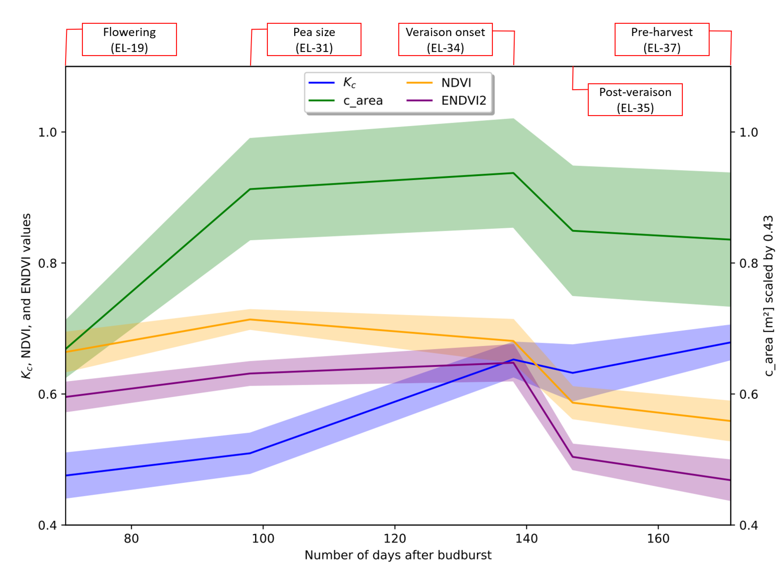
Figure 7.
Correlogram showing the scatter plot, correlation coefficient values and statistical significance (Pearson test: p-value < 0.05 as *, p-value < 0.01 as **, and p-value < 0.001 as ***) between the selected features (spectral and structural) and the crop coefficient.
Figure 7.
Correlogram showing the scatter plot, correlation coefficient values and statistical significance (Pearson test: p-value < 0.05 as *, p-value < 0.01 as **, and p-value < 0.001 as ***) between the selected features (spectral and structural) and the crop coefficient.
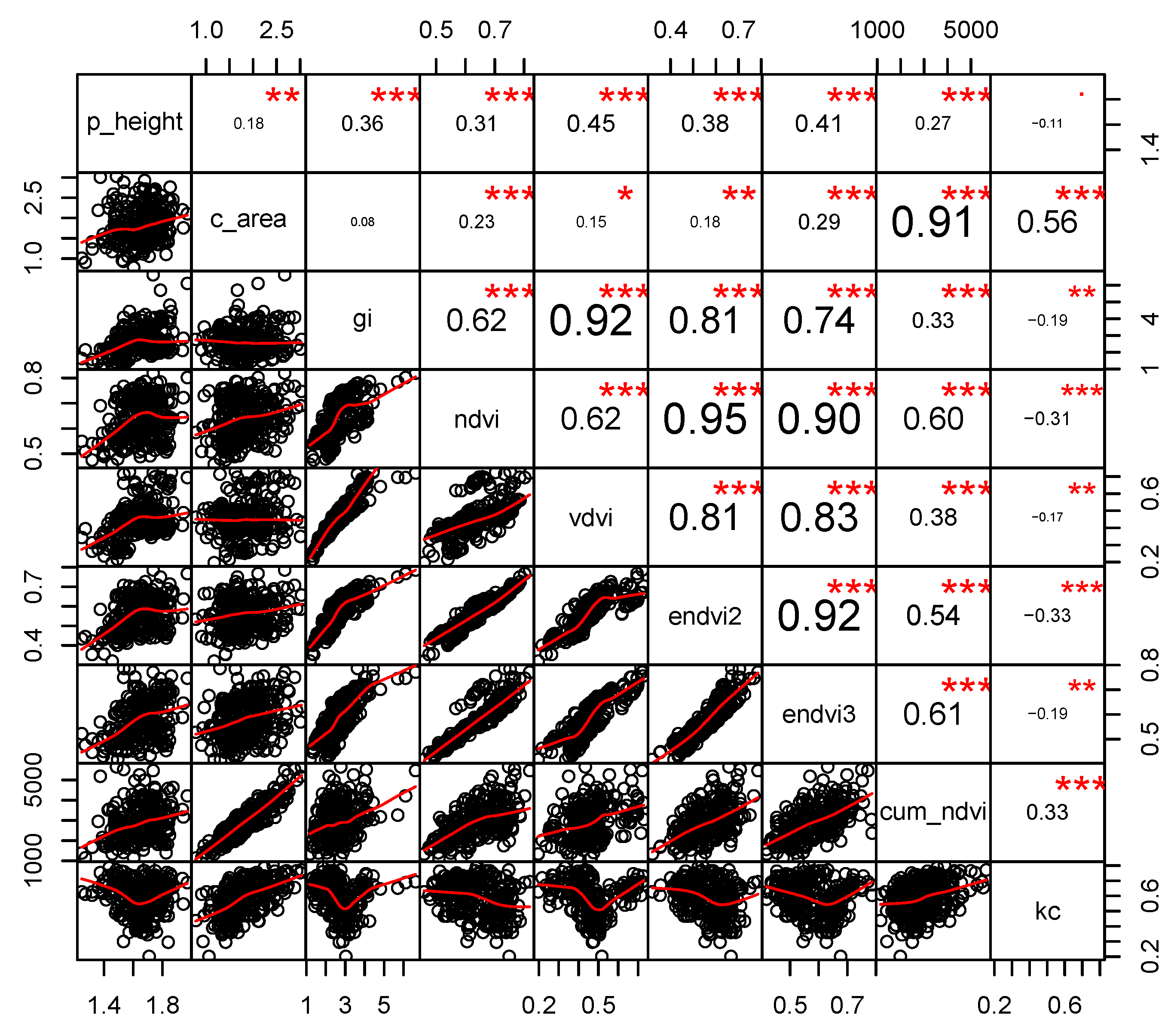
Figure 8.
The map of estimated kc values and at the early season ((left) pane, flowering stage, EL-19) and late season ((right) pane, post véraison, EL-35) of Cabernet Sauvignon.
Figure 8.
The map of estimated kc values and at the early season ((left) pane, flowering stage, EL-19) and late season ((right) pane, post véraison, EL-35) of Cabernet Sauvignon.

Table 1.
The list of spectral and structural features retained after the feature filtering processes, i.e., the removal of non-significant and highly collinear features. Note: R, G, and NIR represent the spectral bands red, green and near infrared, respectively. n and r represent the number of pure-canopy pixels and the spatial resolution of the pixels, respectively.
| Indices | Abbreviation | Formula | Reference |
|---|---|---|---|
| Greenness index | GI | [58,59] | |
| Normalised difference vegetation index | NDVI | [60,63] | |
| Visible-band difference vegetation index | VDVI | [64,65] | |
| Enhanced NDVI #2 | ENDVI2 | modified [66,67] | |
| Enhanced NDVI #3 | ENDVI3 | modified [66,67] | |
| Plant height | p_height | DEM-DSM | [44,61] |
| Cumulative NDVI | cum_NDVI | ∑NDVI | |
| Canopy top-view area | c_area | n × r |
Table 2.
Accuracy of various models used to predict the kc using leave-one-out fit-control. Note the accuracy metrics were derived by applying the model to the unseen testing dataset. Note: AIC in the table heading is an abbreviation of the Akaike information criterion.
Table 2.
Accuracy of various models used to predict the kc using leave-one-out fit-control. Note the accuracy metrics were derived by applying the model to the unseen testing dataset. Note: AIC in the table heading is an abbreviation of the Akaike information criterion.
| Models | R2 | RMSE | MAE | AIC | Most Influential Features |
|---|---|---|---|---|---|
| Generalised linear | 0.528 | 0.074 | 0.061 | −411.7 | GI |
| Generalised additive | 0.594 | 0.069 | 0.055 | −461.7 | c_area |
| Convolutional neural network | 0.619 | 0.072 | 0.060 | na | cum_NDVI |
| Random forest | 0.675 | 0.062 | 0.047 | na | c_area |
Publisher’s Note: MDPI stays neutral with regard to jurisdictional claims in published maps and institutional affiliations. |
© 2021 by the authors. Licensee MDPI, Basel, Switzerland. This article is an open access article distributed under the terms and conditions of the Creative Commons Attribution (CC BY) license (https://creativecommons.org/licenses/by/4.0/).
Share and Cite
MDPI and ACS Style
Gautam, D.; Ostendorf, B.; Pagay, V. Estimation of Grapevine Crop Coefficient Using a Multispectral Camera on an Unmanned Aerial Vehicle. Remote Sens. 2021, 13, 2639. https://doi.org/10.3390/rs13132639
AMA Style
Gautam D, Ostendorf B, Pagay V. Estimation of Grapevine Crop Coefficient Using a Multispectral Camera on an Unmanned Aerial Vehicle. Remote Sensing. 2021; 13(13):2639. https://doi.org/10.3390/rs13132639
Chicago/Turabian StyleGautam, Deepak, Bertram Ostendorf, and Vinay Pagay. 2021. "Estimation of Grapevine Crop Coefficient Using a Multispectral Camera on an Unmanned Aerial Vehicle" Remote Sensing 13, no. 13: 2639. https://doi.org/10.3390/rs13132639
Note that from the first issue of 2016, this journal uses article numbers instead of page numbers. See further details here.