
Applying an Adaptive Signal Identification Method to Improve Vessel Echo Detection and Tracking for SeaSonde HF Radar


1
Institute of Ocean Technology and Marine Affairs, National Cheng Kung University, Tainan 701, Taiwan
2
Department of Marine Science, Naval Academy, Kaohsiung 813, Taiwan
*
Author to whom correspondence should be addressed.
Remote Sens. 2021, 13(13), 2453; https://doi.org/10.3390/rs13132453
Submission received: 27 April 2021
/
Revised: 3 June 2021
/
Accepted: 18 June 2021
/
Published: 23 June 2021
(This article belongs to the Special Issue Remote Sensing for Maritime Safety and Security)
Abstract
:To enhance remote sensing for maritime safety and security, various sensors need to be integrated into a centralized maritime surveillance system (MSS). High-frequency (HF) radar systems are a type of mainstream technology widely used in international marine remote sensing and have great potential to detect distant sea surface targets due to their over-the-horizon (OTH) capability. However, effectively recognizing targets in spectra with intrinsic strong disturbance echoes and random environmental noise is still challenging. To avoid the above problem, this paper proposes an adaptive signal identification method to detect target signals based on a rapid and flexible threshold. By integrating a watershed segmentation algorithm, the subsequent direction result can be used to automatically compute the direction of arrival (DOA) of the targets. To assist in the orientation of the object, forward intersections are integrated with the technique. Hence, the proposed technique can effectively recognize vessel echoes with automatic identification system (AIS) verification. Experiments have demonstrated the promising feasibility of the proposed method’s performance.

1. Introduction
Currently, ocean freight is the most cost-effective method for the international transportation of goods. However, it also gives rise to many maritime security problems. The United Nations Convention on the Law of the Sea (UNCLOS) established 200 nautical miles as the exclusive economic zone (EEZ). This encourages countries to assume greater responsibility for compliance with laws and regulations promulgated in the convention in the respective EEZ. The broad requirement for surveillance plays a greater role in addressing the potential or perceived threats to national security under the terms of UNCLOS [1]. This means that UNCLOS expects maritime activities should be to be safe and legal, but in fact, there are many illegal ships carrying out dangerous maritime activities, so how to implement surveillance is important to authorities. There are two surveillance issues of target within EEZ: cooperative and noncooperative. The former can be defined as a target that operates fully within the law and willing to support the surveillance process, and a noncooperative target refer to those not actively providing information and unwilling to be monitored (e.g., drug trafficking, illegal immigration, piracy, and smuggling). A critical concept remains of maritime domain awareness (MDA) arises for effective understanding of any activity associated with the maritime environment that could impact security, safety and environment.
Maritime Domain Awareness (MDA) is defined by the International Maritime Organization (IMO) as an effective understanding of anything associated with the maritime domain that may affect safety, security, economy, or the environment [2]. The marine domain is defined as all area (e.g., navigable waterway, adjacent, territorial sea) and things (maritime-related activities, people, vessels) [3]. It is necessary to have the ability of conducting effective MDA to solve the challenge of maritime security with effective patrols and surveillance capabilities.
It is clear that the control of territorial waters is not sufficient to ensure the safe movement of goods within EEZ. An EEZ is the area extending 200 nautical miles (approximately 370 km) from territorial waters to the open sea [4]. However, vessels are typically tracked by using automatic identification systems (AISs) or radar [5,6]. To enhance maritime security, international maritime organizations (IMOs) develop strategies, such as international regulations for preventing collisions at sea (COLREGS), vessel traffic services (VTS), AIS, and so on, to increase the safe and efficient flow of traffic at sea. In particular, AIS is an automatic tracking system on board that displays other vessels in the vicinity to aid navigation and collision avoidance, but since then, it can be used for many other applications (e.g., maritime security, fleet and cargo surveillance and control, and search and rescue). In this study, the AIS system operates in the VHF marine time band using broadcast transponder systems, which use self-organizing time division multiple access (SOTDMA) technology. There are two dedicated frequencies or VHF channels; one works on 161.975 MHz–Channel 87B (ship to ship), while the other works on 162.025 MHz–Channel 88B (ship to shore). The AIS includes information about a vessel’s identity, such as its name, ship type, size, and call sign. The messages also include a nine-digit Maritime Mobile Service Identity (MMSI) number that is supposed to uniquely identify ship stations, coast stations, and group calls. Therefore, it is possible to acquire most ship dynamic information by relying on the AIS system. However, AIS is a self-reporting system. If the transmitter is deliberately turned off, messages from the ship will not be received. It is important to consider that many of these techniques suffer from physical limitations, and only the intelligent integration of these different and complementary systems can achieve satisfactory monitoring performance. Currently, a variety of surveillance sensors can be utilized to complement the use of an AIS.
To enhance remote sensing for maritime safety and security, various sensors need to be integrated into a centralized maritime surveillance system (MSS). For an example, the global scale observed via satellite, the approach scale observed by beyond-the-horizon high-frequency (HF) radar, and the local scale observed via line-of-site microwave radars, cameras, and underwater acoustics [6]. The HF radar research is dedicated to developing the due-use surface current mapping and vessel detection capability. Electromagnetic remote sensing is a cost-effective method that is capable of providing complete ocean current field mapping with a shore-based HF radar system [7]. HF radar exploits vertically polarized surface waves in the 3 MHz to 30 MHz frequency range [8,9]. It has the advantage of low power loss with over horizon (OTH) capabilities that can expand the observation distance by hundreds of kilometers by using the sea surface conductivity characteristics to effectively overcome the limitations imposed by the curvature of the earth [10]. This capability aims to bridge a surveillance gap between global satellite with the low update rates and local line-of-sight microwave radars with high update rates. An island-wide HF radar network has been established in Taiwan with the primary aim of monitoring ocean surface currents in near real time. The project is configured to provide a near real-time observation platform for surface current mapping around Taiwan using the SeaSonde® HF Radar system. Most of the sites have been established by the Taiwan Ocean Research Institute (TORI), which is affiliated with the National Applied Research Laboratory (NARL). This institute operates a set of 12 long-range 5-MHz systems and a set of 7 standard 13/24-MHz systems that are included within the network. Two additional long-range stations, i.e., Suao and Habn, are owned by the ROC Naval Academy, which is mainly responsible for the current measurement tasks in the northeastern marine environment. Radar coverage encompasses the surrounding waters of Taiwan. In addition to being able to detect the flow field, it also has the potential for all-weather and large-scale vessel monitoring. HFR is a strong candidate for providing a vessel-monitoring network in any large-scale area. Adding additional applications to develop a ship detection and tracking technique that does not adversely affect the current measurements is a worthwhile endeavor.
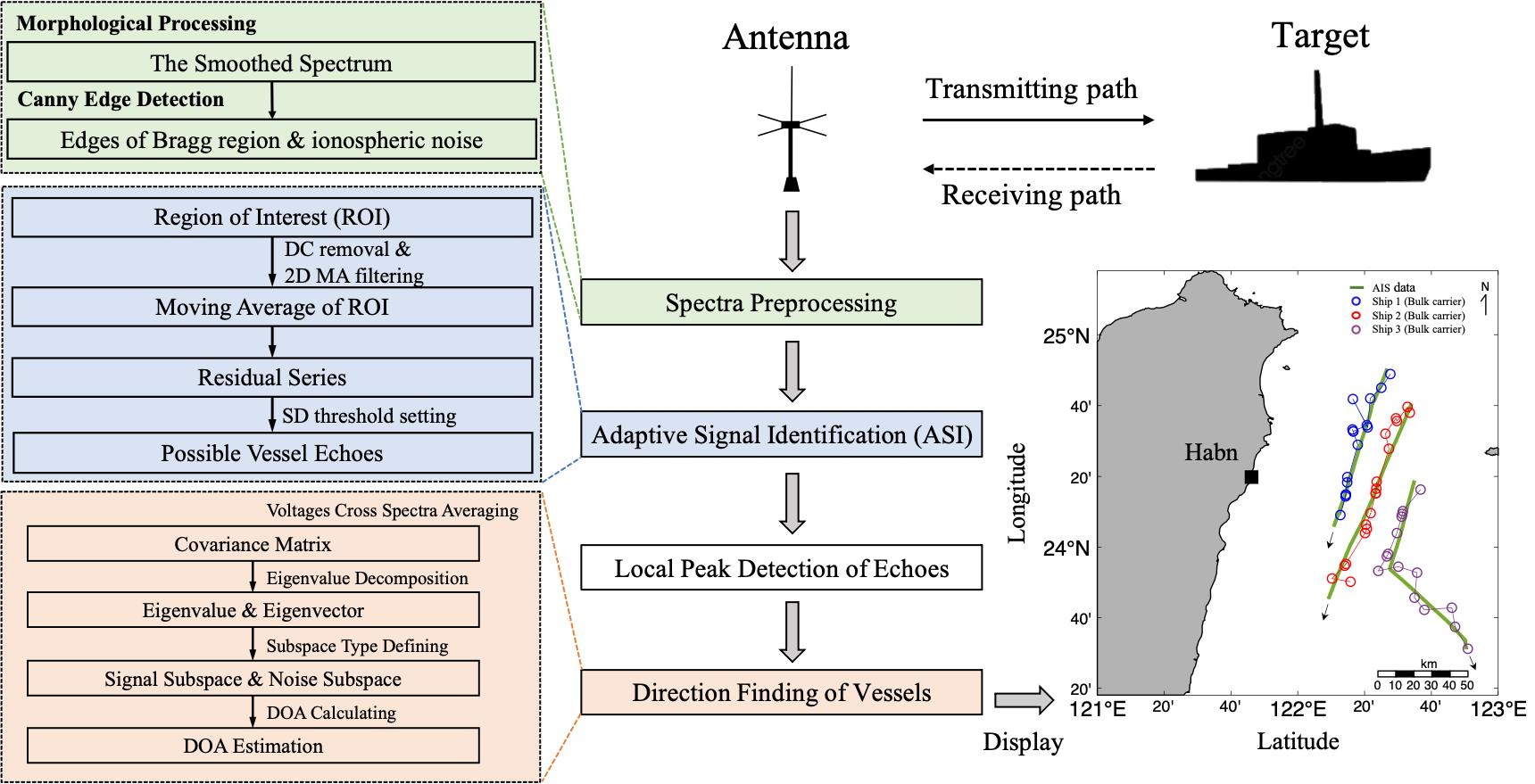
The most important aspect of ship identification involves extracting the signal from the Doppler spectrum. Therefore, this article mainly develops detection techniques that use HF radar ship detection technology. This study improves and develops new detection technologies based on [11]. The measurement technology is then bridged to the direction finding technology by using the watershed algorithm [12]. Target direction determination also plays an important role in the processing of radar signals, and it is possible to accurately collect target position information with a crossed-loop and monopole antenna. For compact HF radar, multiple signal classification (MUSIC) algorithms [13] are employed to estimate the direction of arrival (DOA) of the current and vessel echoes. In principle, this method works by exploiting covariance decomposition to obtain the eigenvector and eigenvalue of signal sources and then attempts to separate the space spanned by measured data into noise and signal subspaces. Once the noise subspace has been estimated, the steering vector orthogonal to the noise subspace can be used to estimate the bearing of targets. This can usually be done by searching for peaks in the MUSIC spectrum.
In the past, most research on high-frequency radar ship detection required the use of complex algorithms or the tuning of radar parameters specifically for ship detection [14,15], which would result in longer detection times or affect their own current mapping tasks. Therefore, the core objective of this study is to establish a set of processes that can quickly and automatically extract suspected ship signals under complex environmental background noise without adversely affecting ocean current measurements. The final integration of the forward intersection method determines the exact location of the ship. In summary, the contribution of this article is to improve the past ship detection algorithm and use the local peak detection algorithm to connect the azimuth recognition technology to make the whole algorithm more complete.
The remainder of this paper is divided into four parts. In Section 2, we introduce the HF radar dataset to analyze ship motion information and review the currently published ship echo signal detection methods. Section 3 describes a new improvement process, including the following algorithms: automatic selection of a region of interest (ROI), adaptive vessel signal identification, the watershed method for local peak detection of echo signals, and the MUSIC algorithm for direction finding of a ship’s echo signal. In Section 4, the analysis process proposed in this study is used to detect the trajectory of three cargo ships in the radar coverage area, and the recognition results are compared with AIS data. Finally, Section 5 offers conclusions.
2. Background
2.1. General Data Description of HF Radar
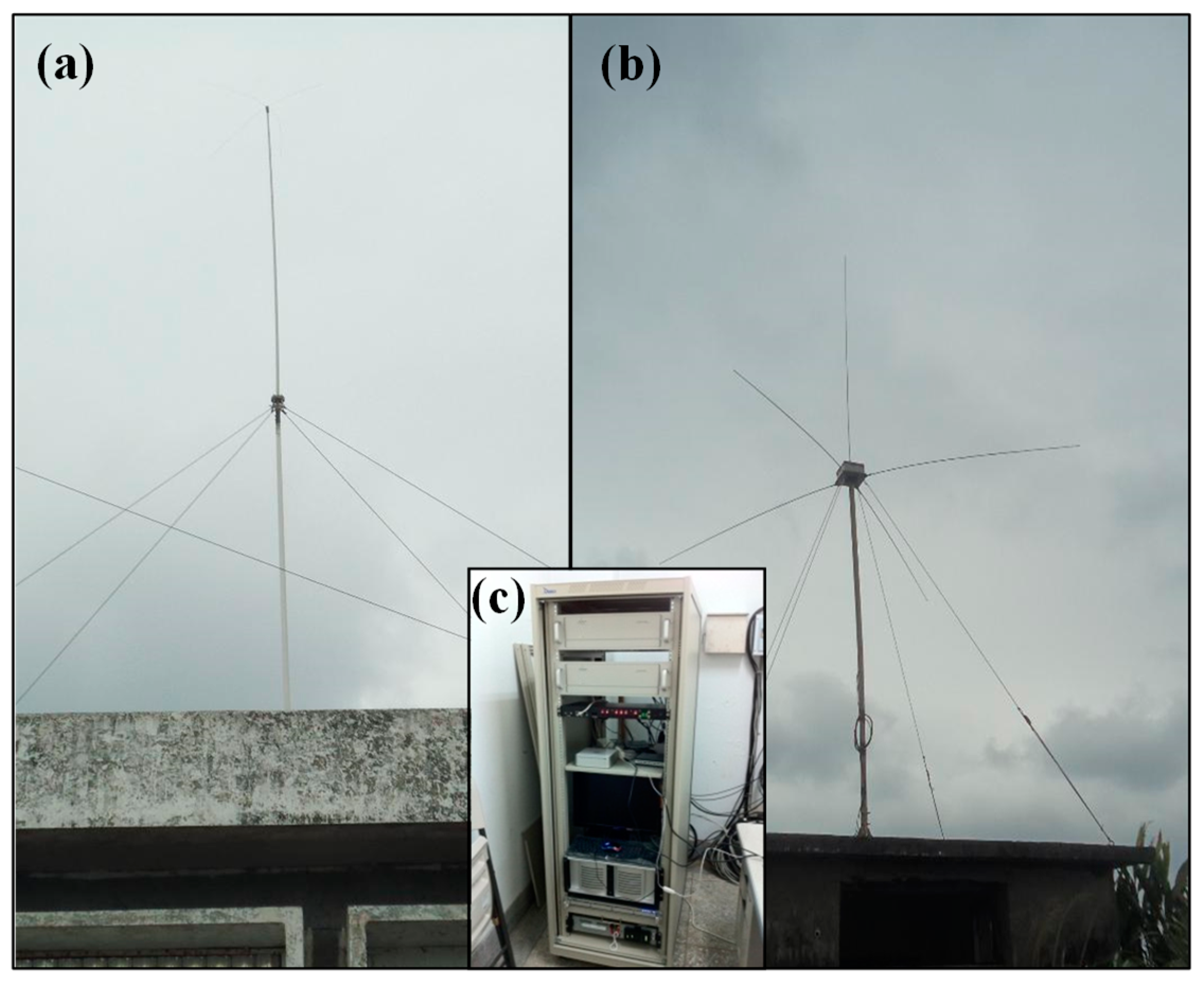
A SeaSonde HF radar station consists of a transmit-receive antenna assembly that is controlled through a control system, as shown in Figure 1. The receiving antenna unit comprises a vertical monopole and two orthogonally mounted cross-loop antennas [16]. The transmitting antenna utilizes a frequency-modulated continuous wave (FMCW) to transmit continuous frequency-modulated radar waves every 0.5 s [17]. Linear frequency modulation refers to the frequency increasing linearly with time in a fixed direction. The radar system receives the echo frequency at any time through the receiver components. The echo signal is compared to the time at which the frequency was transmitted, and the delta time is obtained. It is advantageous for determining the distance between the echo signal target and the radar station [18].
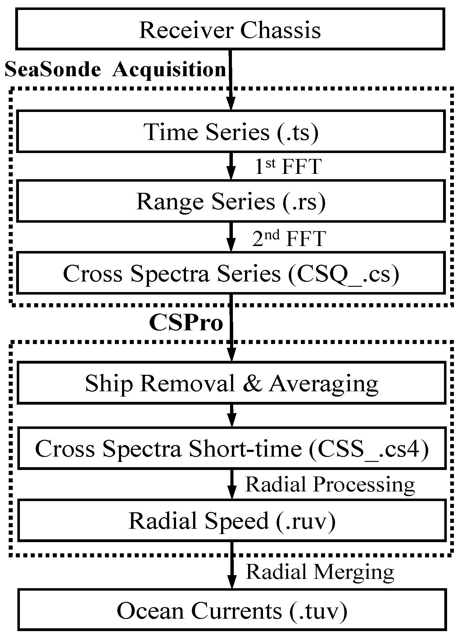
After the radar echo signal is received, the raw time series data (.ts file) received by the radar are first extracted by the first step of the SeaSonde acquisition program, as shown in Figure 2. In SeaSonde acquisition, the range series are obtained by applying the fast Fourier transform (FFT) to the time series. The next step in the data processing procedure is to apply a 2nd FFT to the range series to obtain the cross-spectra series (CSQ. cs). Namely, CSQ is a file type of HF radar, called CSQ file in the field of SeaSonde HF radar, which includes ocean current information, noise interference, and original information of Doppler energy spectrum of ship echo. The interlaced spectral sequence belongs to the original Doppler spectrum, which contains ocean current information, noise interference, and the original Doppler spectrum information of the ship echo. Therefore, the CSPro program uses the exponential smoother for noise reduction, such as ship echo signals. The use of exponential smoother smoothing will result in a more accurate short-spectrum short-time cross-time (.cs4 file) for subsequent estimation of the radial flow velocity [19]. The purpose of this study is to detect and track ships. To prevent CSPro from filtering out ship signals, this study processes an original cross-spectra series containing the ship signals.
2.2. Detection of Vessels in the Radar Echo Signals
Confronting the challenges of implementing marine ship management, HF radar is a highly promising sea area monitoring tool [20]. In recent years, research on ship detection and tracking using HF radar has not only been proposed but has also been effectively used for vessel detection at OTH distances [21,22,23]. Some studies use the probability of detection (Pd), false alarm (Pfa), and other variation parameters to evaluate the ship detection performance [24]. The relationship between Pfa and Pd under different SNR values was analyzed, and it was found that high detection rates may be accompanied by high false alarm rates. Due to some known factors, HF radar has some deficiencies in terms of SNR-related ship detection, and effective improvement of these shortfalls can be achieved by using multiple observation points or different observation frequencies.
In addition to using different frequency and multipoint observations, some data processing methods have been proposed to improve the identification of ship echoes in HF radar signals. To distinguish the high-energy signals from background noise, two detection algorithms, i.e., infinite impulse response (IIR) filters and two-dimensional median filters, are used to calculate the background signal level, and then a fixed threshold is added to the background as a ship detection method [14]. Among the various types of false alarms, AIS is utilized to determine real ships in a multitarget environment.
In the same year, Vesecky, J. F (2010) [25] mentioned that the HF radar and AIS ship detection models developed in the past estimate the signal-to-noise ratio (SNR) as a function of range, including the pipeline propagation of AIS radio signals. However, the high variability of HF prevents ships from detecting ship echoes. This is due in part to the aspect dependence of ship radar cross-section and to the presence of clutter bands at known Doppler shifts from both the ground and ocean waves [25]. Based on the above interference, the Kalman filtering approach is used to recognize ship signals without changing the radar hardware equipment in the exclusive economic sea area of the United States. It is a highly efficient recursive filter. The dynamic state of the ship can be estimated from spectral data containing noise. The researchers concluded that tracking algorithms can be applied in back-end processing software algorithms without modifying the existing radar hardware. However, Doppler spectrum limitations exist. It is not easy to recognize ship movement in a blind zone. Therefore, multiband HF radar was used to detect and track ships in the East China Sea, and AIS data were used to verify the results, confirming that multiband detection technology can prevent ship signals from being hidden in blind spots. The effectiveness of HF radar to detect ships is related to the ship size [26].
This research focuses on radar parameter adjustment and compares the ship detection rates of the two IIR and median filter methods when used to detect four ships of three different types, namely, a tugboat, two cargo containers, and a tanker, in the Sea Bright area of New Jersey [27]. The adaptive detection technique (ADT) establishes a threshold surface that can be adapted to noise, screens out ship signals higher than noise, and then uses AIS for verification [11]. The ship signal analysis method was developed to remove the distance sequence data output from the CODAR original system, and then the median filter is used to calculate the background noise [28]. The noise reference value of the signal-to-noise ratio (SNR) is used to filter out the ship signal based on an SNR greater than 20, and then it uses the Kalman filter to track the trajectory and reduce the false alarm rate. A multi-target tracking (MTT) strategy was proposed in [8], which refers to the problem of jointly estimating the number of targets. The states or trajectories from noisy sensor measurements are based on the joint probabilistic data association (JPDA) rules. Target detection is performed in the FFT domain using 3D (range-azimuth-Doppler)-ordered statistics and a constant false alarm rate OS-CFAR algorithm [29].
Principal component analysis was used to enhance the signal in the Doppler spectrum, and wavelet suppression was applied to suppress the noise and improve the SNR of the ship echo. Finally, on a Doppler spectrum filled with multiple targets, targets were extracted using adaptive threshold detection [30]. An FMCW radar was used to monitor the ship navigation with sixteen vertical dipole antennas and 16 receiving channels [31]. That study proposed a procedure for ship echo identification from the conventional RD map. By employing three beamformers, linear Fourier, directionally constrained minimum power (DCMP), and norm-constrained DCMP (NC-DCMP) algorithms were employed to produce a range-angle (RA) brightness distribution map that is different from the conventionally used range-Doppler (RD) spectra in ship detection.
2.3. Adaptive Detection Technique
Adaptive detection technology is an established technology, and the contribution of this article is the improvement of ADT. The following briefly introduces the ADT algorithm. The first step of the ADT is to apply a 2D moving average (MA) filter to CSS, which is known as an RD map, to reduce random noise while retaining the primary energies of the Bragg peaks, the zero Doppler frequency, and any moving targets. A residual series (RS) can then be derived from the difference between the raw RD map and the MA of the CSS. To identify the signals of moving targets, different small regions of interest (ROIs) of the RS can be independently designated for further analysis. Finally, an adaptive threshold surface based on the standard deviation (SD, σ) of the residual series should be set in each ROI to differentiate possible vessel echo signals from the noise floor. Although the above algorithm has been proven to effectively identify ship signals, there are still some intermediate steps that need to be improved and strengthened in actual operation. In addition to the ships' reflected signals and random noise, there will also be other reflected signals remaining in the residual, such as the echo energy at the Bragg peaks and zero frequency. This will affect the selection of the optimal window size of the 2D MA filter in the ADT method, so we propose a revised version of the improvement process in this article and assign a new name, i.e., adaptive signal identification (ASI), to distinguish it.
In subsequent experiments, we found that the moving window (MW) approach, which is a 2-D shift filter with different sizes for the Doppler spectrum, is quite correlated with environmental noise. The noise index measurement mechanism is described in references [32,33], following the principle of the above paper to select the area from the second-order Bragg peak outward to the two ends of the side and compute the average spectral energy values as the noise index in this area. The expected threshold curve surface for source separation fluctuates with the noise level trend and is related to the terrain near the receiving antenna, the radar detection distance, the ionosphere, and many other factors. The above variables affect the smoothness of the filtering used in ship detection, as shown in Figure 3. The axis of the abscissa denotes the size of the MW, and the ordinate represents the noise index. The result shows that the noise index is high, and the corresponding MW is relatively small based on over 2590 data points from CSQ in October 2013. The R-squared value is as high as 0.70666 based on linear regression analysis. This approach attempts to model the relationship between two variables by fitting a linear equation to observed data. The main reason for the high correlation is that a rugged threshold plane must be generated by a small MW to further filter out suspicious ship signals.
In addition, a high-energy signal at the central frequency in the HF radar Doppler spectrum is called a direct current (DC) signal, which reflects energy from islands or targets that are not in relative motion with the radar station. The DC will affect the MW required for vessel detection. Therefore, it is necessary to improve the original ADT process by directly processing the entire distance Doppler spectrum covering different environmental noise characteristics. Although the ADT automatically selects a suitable filtering surface with noise, removal of the energy with a greater impact in the Doppler spectrum in advance will help in the implementation of the ship detection algorithm.
3. Methodology
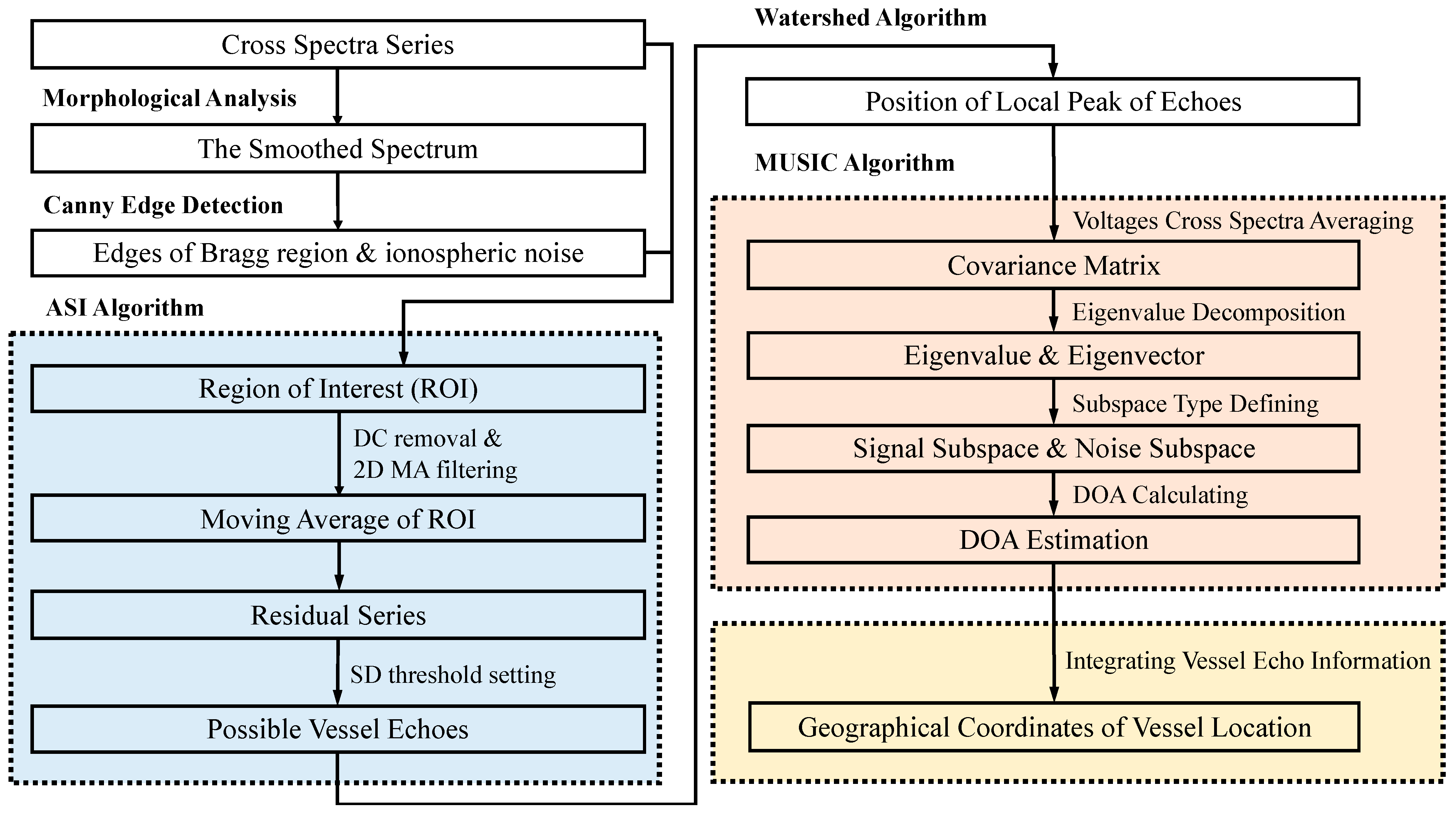
In the present study, we adjust and optimize the ADT analysis procedure to enhance the ability of ship signal extraction along with environmental background noise and echo distance and rename the new process the ASI algorithm. The ASI, shown in the flowchart of Figure 4, still retains the main steps of the original ADT but moves the step “region of interest (ROI)” to the front. In addition, before performing the ASI algorithm, two steps, “Morphological Processing” and “Canny Edge Detector,” are employed to determine the influence range of the Bragg region and remove the energy of the Bragg resonance effect from the cross-spectra. The advantages of using ASI instead of ADT include avoiding the subjective setting of the experience parameters and making it easier to execute Doppler spectrum signal acquisition according to the local conditions.
After using the ASI algorithm to differentiate possible vessel echo signals from the noise floor of the cross-spectra, there are three procedures for the subsequent operationalization process. A watershed method is used to automatically find the digital values of the range and Doppler frequency corresponding to the peak of the suspected vessel echoes. Then, the “Position of Local Peak Echoes” provides the voltage value information of vessel echoes for the subsequent MUSIC algorithm to determine the azimuth of the vessel. The final step is to visualize the ship dynamics on a map to determine the spatial coordinates of the ship signal through the distance and azimuth of the ship signal provided by ASI and MUSIC, respectively.
3.1. Preprocessing of the ASI Algorithm
The wave motion performance will produce first-order and second-order resonance scattering on the Doppler spectrum in a fixed range, which will exhibit dominant peaks, called Bragg peaks, as shown in Figure 5a, on the left and right sides of the Doppler spectrum. In addition to these two significant echo energies, ionospheric noise (Figure 5a) may also be involved in the Doppler spectrum. The strong interference energy mentioned above will affect the subsequent identification of ship signals, so we add two processes, i.e., morphological analysis and Canny edge detection (Figure 4), to eliminate their influence before performing ASI.
The first step is to specify the ROI to avoid interference. It is also beneficial for effectively improving the time consumption and evaluating the accuracy of suspicious ship echoes. Actually, the signal is not homogeneous, and spike signals, such as the delta function, often appear in the Doppler spectrum. Using edge detection directly to find the edge of the strong echo will cause considerable noise to be detected at the same time and cannot be clearly defined as an ROI. First, we need to reduce the noise of the cross-spectra series but still maintain the shape and characteristics of ship echoes, so we adopt the closing operator (Equation (1)) in mathematical morphology to highlight the shape features of Bragg peaks and ionospheric noise. Morphological analysis probes a digital image with a predefined simple shape, called a structuring element, and then draws a conclusion regarding how effectively this shape matches the features of the image. The closing of image A (Figure 5a) by structural element B is obtained by the dilation of A by B, followed by erosion of the resulting structure by B, as shown in Equation (1). Operator dilation is used to connect the regions by expanding the components of an image, and operator erosion is used to remove noise by shrinking the components of an image [34].
where A is the spectrum data, B is the structural element, ⊕ is a dilation operator, and Θ is an erosion operator.
Figure 5a is a raw Doppler spectrum at a specific time. After the closing operation of Equation (1) is performed, the result shown in Figure 5b can be obtained. The advantages of the closing operation are filling small holes in the Doppler spectrum, connecting adjacent objects, and smoothing boundaries without significantly changing the area, so the shapes of the Bragg peaks and the ionospheric noise in Figure 5a can be strengthened, and their borders can be highlighted, which will facilitate subsequent edge detection.
The next process is to perform edge detection on the affected areas of the Bragg peaks and ionospheric noise. The tool used is a Canny edge detector, which uses a multistage algorithm to detect edges of images with noise suppression at the same time. The first step is to apply a Gaussian filter to smooth the image to reduce noise and unwanted details and textures, and then the gradient operators are used to find the intensity gradients of the smoothed image. The second step is to apply nonmaximum suppression to find the locations with the sharpest change in the intensity value to eliminate spurious responses to edge detection, and then select high- and low-threshold values of the previous result to determine the potential edges. After using the edge detector to mark the influence ranges of Bragg peaks and ionospheric noise (Figure 5c), an ROI (the red box in Figure 5c) with no interference from the aforementioned noise can be selected.
3.2. Adaptive Signal Identification Algorithm
The steps of the ASI algorithm and its four consecutive stages of output are shown in Figure 4, and the schematic implementation results are illustrated in Figure 6. The first step is to select an ROI (Figure 6a) from the CSS that is not affected by Bragg peaks and ionospheric noise and convert the Doppler shift frequency axis of the spectrum into a radial velocity axis. However, there is still a strong echo energy at zero velocity in Figure 6a, which will affect the analysis results of subsequent steps. Therefore, referring to the processing method of the SeaSonde HF radar system, a step called DC removal is performed to eliminate the strong spectral energy near the zero velocity. In reference to [19], the incoming data (raw Doppler spectrum) within 2 Doppler bins (radial velocity) totaling five bins around the DC Doppler bin are set to be the average value of these two bins at the edges of this DC region for all ranges, and the processing result is shown in Figure 6b.
Next, we refer to the ADT algorithm and perform a 2D moving average filter on Figure 6b to obtain an adaptive average surface, as shown in Figure 6c. This step is similar to ADT, which can filter out random noise but retains the echoes of the moving targets of Figure 6a. However, the difference between ASI and ADT is that there is no longer ionospheric noise, high energy at the Bragg peaks, and zero Doppler frequency in the chopping surface in Figure 6c. For the definition of 2D MA and how to use it, please consult the literature [11]. To determine the best size of the 2D MW, we consider various windows with the sizes (m × n) of 3 × 3, 3 × 5, 3 × 7, 3 × 9, 3 × 11 … to 3 × 301, where the first and second numbers represent the numbers of the range and radial velocity cells, respectively. These 150 windows are used to evaluate the kurtosis and skewness of the histogram of the corresponding residual series (Figure 6d), which is the difference between Figure 6b,c. From the change trends of the skewness and kurtosis of the histograms in Figure 7, which show the deviations from the normal distribution for various sizes of 2D MAs, we can select the window size that is most suitable for Figure 6b.
Skewness is a measure of the symmetry in a distribution. Kurtosis is a measure of whether the data are heavy-tailed or light-tailed relative to a normal distribution. The standard normal distribution has a skewness of 0 and a kurtosis of 3. It is near normal if skewness ranges from −1 to 1 and the kurtosis ranges from 2 to 4. Figure 7a shows that the skewness rapidly approaches −0.5 and the kurtosis rapidly approaches 2 when the window size gradually increases. However, when the length of the radial velocity cell is greater than 50 (that is, the window size is 3×50), the kurtosis value does not change markedly; however, when it is greater than 100, the kurtosis value gradually moves away from 3. Hence, when the kurtosis value is increased from 50 to 100, if the degree of change in the kurtosis value is lower than a specified threshold, the kurtosis value can be considered to have reached convergence. Therefore, we believe that the change in the kurtosis curve in Figure 7a has stabilized when the slope change in the kurtosis curve reaches the 1% threshold (the red line in Figure 7b).
A ship signal can be determined with the standard deviation after obtaining the best MW through the abovementioned rigorous approach. Next, the watershed division method is used to distinguish the regions in the Doppler spectrum. This method initially distinguishes whether the local front values are independent systems. The preliminary results are shown in Figure 6f. Each color block represents the independent system of each zone, and the maximum value of each zone is selected. Compared with the original image, it can be clearly observed that each strong echo is automatically searched. In this way, the positions of the range cell and Doppler bin are obtained. The MUSIC algorithm relies on the above local peak position voltage spectrum signals for direction determination. Although the most widely known watershed algorithm has an excessive segmentation problem, using the algorithm proposed in this paper to preprocess spectra can effectively reduce the problem of excessive segmentation of the watershed algorithm.
3.3. Watershed Algorithm
This section introduces the watershed algorithm in detail, which is an important algorithm in the image segmentation algorithm. It has been widely used in the process of image processing because of its good edge detection ability and its ability to obtain relatively different regional characteristics [12]. The basic idea of the watershed algorithm is to treat grayscale images as elevation images. The grayscale change in the image is representative of topographic relief. Assuming that water is continuously injected into the area, the lower-lying position will be inundated first, and the area that is submerged as the water level rises will continue to increase. When the water level reaches a certain height, the two collection basins will be connected and will merge into a single area. At this time, a water dam should be established between the two collection basins to prevent merging of the areas. In other words, using the gray value distribution feature of the pixel, each region that conforms to the feature is divided to form a boundary to form a watershed. The largest feature of the algorithm is image segmentation based on the similarity between pixels. The algorithm improves the defect of ignoring the spatial relationship of pixel points in traditional edge detection and contour detection. This paper integrates the watershed algorithm with the ASI algorithm. The specific steps for the process are as follows:
- The ASI algorithm derives suspected ship signals from the original Doppler spectrum, and it is essential to remove the recorded voltage value of the local peak for direction determination. This paper uses the watershed algorithm to automatically distinguish each region in the Doppler spectrum and to select local peaks from the basin. In the first step, the image gradient in the Doppler spectrum is calculated, the region with the smaller gradient value is obtained as the collecting basin through the image gradient, and all the pixels in the same collection basin are obtained by searching in eight directions in the process of acquiring the collection basin. Each local minimum and its area of influence is called a basin, and the boundaries of the basin form a watershed.
- The boundary pixels of the collection basin are judged in eight directions to detect whether the pixels can be submerged, and the image collection basin and the collection basin boundary pixels are recalculated. Finally, the maximum value of each region is automatically selected from each watershed spectrum. This method can be used to obtain the vertical and horizontal axis positions of the signal peak, which can provide voltage value information for subsequent direction-finding algorithms.
3.4. Multiple Signal Classification Algorithm
Schmidt (1986) found the relationship between signal observations and antenna patterns in the cross-spectrum of high-frequency radars. The received signal voltage is modelled as a linear combination of the incident signal, antenna response, and noise. Then, it is used in the MUSIC algorithm [13].
The results of the ASI algorithm integrated with the watershed algorithm will automatically provide the voltage spectrum value of the suspected ship signal to MUSIC. In addition to the voltage signal, this algorithm also requires inputting of the antenna pattern, which describes the response of the receiving antenna to the signal source and more accurately determines the direction of the signal. The directional sensitivity of the loop receiving antenna is based on the amplitude and phase of the signal source in the pattern [35]. The incident wave at each angle generates different amplitude ratios and phase differences among the three sets of receiving antenna patterns. Figure 7a shows the actual antenna pattern of the Habn HF radar station. The orange solid line is the pointing angle of loop1. The estimated range is 30 degrees to 150 degrees. The degree is zero degrees clockwise from true North.
The basic idea of the MUSIC algorithm is to decompose the covariance matrix of the output data of any array and divide the observation space into a noise subspace composed only of noise and a signal subspace composed of noise and signals [36]. Then, the orthogonality of these two subspaces is used to construct a spatial spectral function and search for the DOA of the detection signal through the spectral peak. MUSIC is a representative structural analysis method with good angular resolution. Under certain conditions, the MUSIC algorithm is a one-dimensional implementation of the maximum likelihood method with a performance similar to the maximum likelihood method. Therefore, we can estimate the azimuth of the ship on the Doppler spectrum through the MUSIC algorithm.
The DOA plays an important role in array signal processing, and its application range is quite critical when dealing with radar signals. It can help remote sensing instruments identify the target location accurately. The SeaSonde system uses an omnidirectional antenna with three sets of collocated antennas for simultaneous reception and records the echo energy with a voltage value. The DOA solution method was proposed by Schmidt [13] to solve the main orientation of the target by analyzing the characteristics of each set of antenna self-spectra and the other two sets of antenna cross-spectra and the antenna pattern (Figure 8a). This study uses the MUSIC algorithm to obtain the DOA solution of the target. The most important core technology of MUSIC is to define a subspace type definition. After eigendecomposition, the eigenvalues and eigenvectors are further divided into signal subspaces and noise subspaces. The orthogonality of the subspaces can be used to estimate the direction of the signal source. The last step is to find the target DOA function of the signal source using Equation (2), as follows:
where En is the eigenvector of the noise subspace, A(θ) is the steering vector of the antenna, and A* is the transposed matrix of A. Additionally, the single-angle or double-angle hypothesis is used to define the signals received in different directions, and the antenna steering vectors are brought into the function individually. Due to the orthogonal characteristics of the noise subspace and the signal subspace, when approaching the correct signal source angle, the component of the projection in the signal subspace will be heavier, and the product with the noise subspace will approach 0. In the DOA formula, the denominator will be close to 0 in the antenna steering vector and orthogonal to the noise subspace. With this feature, MUSIC will produce a peak at a specific angle in the DOA solution (Figure 8b), thus effectively estimating the signal source.
3.5. Map Information Display
Compared to those of the general X-band radar, the results of target detection with HF radar are not intuitive. Therefore, the final step in the entire ship detection process is to visualize the ship dynamics on a map using the latitude and longitude of the known radar station and the distance and azimuth of the target relative to the station. The coordinates of the target object in front are determined, and the detailed formulas are as follows:
ϕA is the latitude of point A; ϕB is the latitude of point B; λA is the longitude of point A; λB is the longitude of point B; R is the distance between the middle of point B and point A; θ is the azimuth of point B with respect to point A.
The ASI and MUSIC algorithms provide the distance and azimuth information required for the above equations. The ASI captures the suspected ship echoes in the spectrum and then uses the watershed algorithm to select the voltage spectrum of the ship echoes for direction determination using the MUSIC algorithm. Finally, expressions (3) and (4) are used to calculate the longitude and latitude of the target and present the estimated points on the map. The ship’s trajectory is obtained by detecting the target continuously over time. A comparison with the AIS is then carried out to confirm the feasibility of the algorithm for ship tracking.
4. Experimental Results
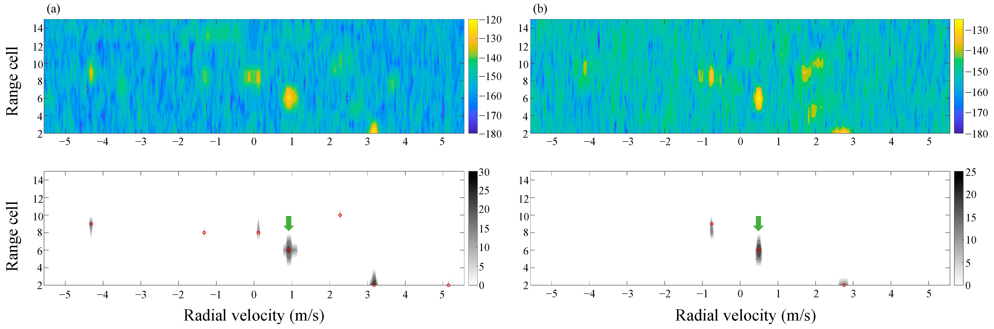
This study took large ships sailing in the eastern seas of Taiwan from 29 October 2013 to 31 October 2013, as an example. Figure 9 shows the echo of a target vessel detected continuously by ASI. The top half of the figure is the original Doppler spectrum, and the suspected ship echo signal can be obviously obtained via ASI processing. The name of ship 1 is May Oldendorff, ship 2 is Berge Lyngor, and ship 3 is Fakarava. The length and width of the selected bulk carriers are 300 m (984 ft) and 50 m (164 ft). The ships have large superstructures and high mast elevations, which have a good detection effect with HF radar. The green arrow is the location of the target, which was identified by AIS. The horizontal axis of the echo is the radial velocity, with positive values indicating that the ship is approaching the radar station. The signs of the target's proximity to the radar station can be observed at two consecutive time points. The voltage values of the local peaks of the echoes are extracted by the watershed algorithm and returned to the direction-finding method for calculation.
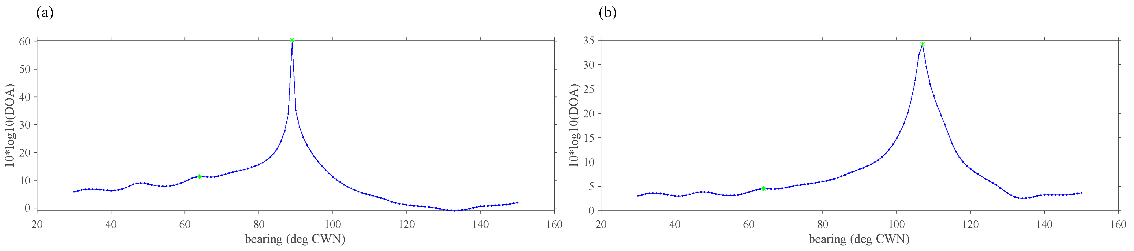
The MUSIC algorithm was added to the ship identification technique to search for the DOA, as shown in Figure 10, showing the bearing of the target relative to the Habn station. The horizontal axis is the DOA, and the vertical axis is the DOA function. We can observe the ship moving from 105 degrees to 87 degrees in azimuth from two consecutive time points. Subsequently, the radar site can be used to effectively estimate the position of different vessels by the detection method proposed in this study. The actual AIS track displayed by the green line is shown in Figure 11. Ship 1 and ship 2 sailed from north to south according to the AIS data. The other vessel named ship 3 navigated from north to south and then turned east. In this paper, the proposed HF radar ship detection algorithm is used to analyze the data from the long-distance Habn radar site, and the three ships are locked in for long-term tracking. The circle is the exact position of the ship estimated through the entire ship detection algorithm. The above position mainly uses ASI to identify suspected ship signals in the Doppler spectrum after selecting the ROI by morphology and canny edge detection. Then, the local peaks are filtered out using the watershed algorithm and are entered into the MUSIC algorithm to extract the DOA information. The AIS data are then used to assist in identifying that the radar result is indeed a vessel. Finally, the distance obtained by ASI and the bearing information estimated by MUSIC are brought into the formula to estimate the actual position of the vessel.
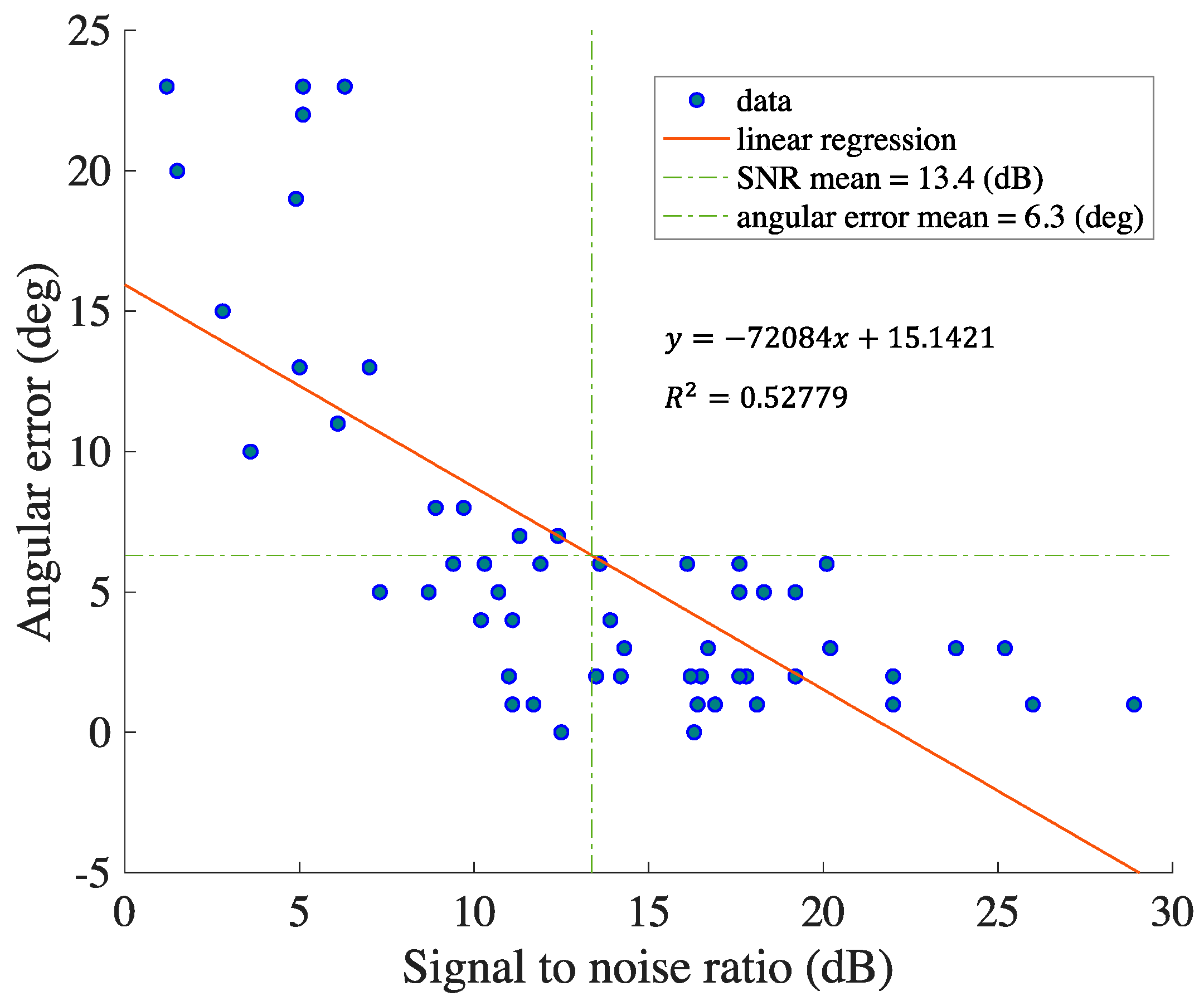
Therefore, this article analyzes the SNR value of each detection point and its angular error (Figure 12). The horizontal axis is the SNR value, and the vertical axis is the angular error. The average SNR value and the angular error value are 13.4 dB and 6.3 degrees, respectively (the green dashed lines on the vertical and horizontal axes in the figure). The r-square statistical value obtained from linear regression of this dataset is 0.52779; typically, a value greater than 0.5 is considered acceptable [37,38].
5. Discussion
The detection results approximately match the actual ship trajectories. The trajectories of ship 1 and ship 2 are very similar and nearly coincide with the actual AIS trajectory data. Only a few estimated positions are less accurate in the figure. This study speculates that this may be related to the lower SNR values at specific times. In addition, the tracking performance of ship 3 was fairly good until it turned to the southeast. However, the relative error increased when the ship changed course. The possible reason is that the RCS provided by the stern facing the radar station decreased, resulting in a weak signal strength. The RCS is a measure of how well an object is detected by radar. The influencing factors include the material of the target, the absolute size of the target and the reflected angle. Moreover, it can be further confirmed that the smaller the SNR is, the larger the angular error, which will cause a larger error in the exact position estimate of the ship according to the analysis of the SNR value and angular error.
6. Conclusions
This paper makes three contributions. The first contribution is that it solves the problem where the strong echo energy of the ADT method interferes with the selection of the optimal window size of the filter, including the Bragg peak and the echo energy at zero frequency. A revised version of the improved process is presented, and a new name, i.e., ASI, is given to distinguish it. ASI has the ability to quickly and automatically extract ship signals under complex environmental background noise without adversely affecting the sea surface current mapping. Namely, the ASI algorithm is a kind of vessel identification method based on image processing and statistical analysis. There are two advantages. The first one is that the algorithm can establish an appropriate threshold surface for vessel signal extraction according to the characteristics of environmental noise. There is then no need for too many manual parameter settings. The following paragraph describe the procedure of the ASI algorithm. The second contribution is that the whole process was automated by adding morphology and edge detection methods to assist the automatic ROI selection before the ASI is employed. To provide subsequent information on direction-finding techniques, this paper adds the watershed algorithm used for automatic peak detection after the ASI is employed. These new technologies are processes that are not included in ADT. The most well-known problem of the watershed algorithm is oversegmentation. This article has confirmed that in the past, if the watershed algorithm directly targets the frequency spectrum, there will be excessive oversegmentation. However, after the Doppler spectrum is processed by ASI, a large amount of noise will be filtered to retain the main signal of the suspected ship, and then the watershed algorithm will be used to divide the Doppler spectrum without oversegmentation. The last contribution is that the case analysis also initially confirmed that the HF radar ship detection algorithm has the ability to identify large ships and can carry out long-term tracking. The smaller the SNR is, the larger the angular error obtained. Additionally, the feasibility of the algorithm is confirmed by comparing the AIS data, and more cases and ship sizes can be examined in the future.
The whole algorithm can adjust the appropriate signal filtering threshold with the environmental background noise and echo distance to more effectively extract the possible ship echo signals and avoid the subjective setting of the empirical parameters. Time signal acquisition was performed, and the results were output to the map for visualization. This expected result not only enhances the technical capability of existing HF radar systems to detect and track ships moving at sea, but also demonstrates the ability of HF radars to act as a strain mechanism for long-range warning systems.
The detection performance of radar can be evaluated by the false alarm rate. In future research, a large number of samples will be quantitatively studied based on the method proposed in this paper. This work is divided into three main parts. The first step is to establish a large number of AIS ship databases. The second step is to use ASI and MUSIC to obtain information (distance, radial velocity, bearing) on the suspected ship signals on the Doppler spectrum. The last step is to establish a comparison system to compare the radar and AIS data. Then, the confusion matrix is used to evaluate the detection performance of the system. The four indicators in the confusion matrix are individuals. In fact, the false alarm rate means that the radar has detected a ship, but there is actually no ship (AIS has no data), that is, the result is a false negative (FP). The confusion matrix can even further calculate the detection rate, accuracy rate, and recall rate. Therefore, it is expected that in future research, based on the developed technology, the problem of false alarms that is common in vessel detection can be solved in a quantitative manner.
Author Contributions
Writing—original draft, Y.-R.C.; Writing—review & editing, Y.-R.C., L.Z.-H.C. and Y.-J.C.; Conceptualization, L.Z.-H.C., Y.-R.C.; Data curation, Y.-R.C. and Y.-J.C.; Formal analysis, Y.-R.C.; Funding acquisition, L.Z.-H.C., and Y.-J.C.; Investigation, Y.-R.C.; Methodology, Y.-R.C., and L.Z.-H.C.; Resources, L.Z.-H.C. and Y.-J.C.; Software, Y.-R.C. and Y.-J.C.; Supervision, L.Z.-H.C., Y.-J.C.; Visualization, Y.-R.C. All authors have read and agreed to the published version of the manuscript.
Funding
This research was funded by the Ministry of Science and Technology, Taiwan under grants 109-2221-E-006-101 and 108-2611-M-012-002 and Ministry of Education, Taiwan under grants PEE1090492.
Institutional Review Board Statement
Not applicable.
Informed Consent Statement
Not applicable.
Data Availability Statement
The data presented in this study are available upon request from the corresponding author. The data are not publicly available due to security issues.
Acknowledgments
We thank all the scientists and principal researchers who prepared and provided the research data. Thank Yiing-Jang Yang from National Taiwan University (NTU), Jian-Wu Lai from Ocean Affairs Council (OAC), Lee-Chung Wu from Coastal Ocean Monitoring Center (COMC) for technique support. Thank Paduan and Cook from Naval Postgraduate School (NPS) for discussion and support especially. We thank Harbor and Marine Technology Center, Institute of Transportation, Ministry of Transportation and Communications for providing the AIS data used in this study. Finally, we also thank the anonymous reviewers for their constructive observations.
Conflicts of Interest
The authors declare no conflict of interest.
References
- Moutray, R.E.; Ponsford, A.M. Integrated maritime surveillance: Protecting national sovereignty. In Proceedings of the International Conference on Radar (IEEE Cat. No. 03EX695), Adelaide, Australia, 3–5 September 2003; pp. 385–388. [Google Scholar]
- International Maritime Organization. Amendments to the International Aeronautical and Maritime Search and Rescue (IAMSAR) Manual. Available online: https://www.irclass.org/technical-circulars/amendments-to-the-international-aeronautical-and-maritime-search-and-rescue-iamsar-manual/ (accessed on 26 May 2021).
- Bueger, C. From dusk to dawn? Maritime domain awareness in Southeast Asia. Contemp. Southeast Asia 2015, 37, 157–182. [Google Scholar] [CrossRef]
- United Nations. Law of the Sea, Part V—Exclusive Economic Zone; United Nations: New York, NY, USA, 2011. [Google Scholar]
- Kazimierski, W.; Stateczny, A. Radar and automatic identification system track fusion in an electronic chart display and information system. J. Navig. 2015, 68, 1141. [Google Scholar] [CrossRef]
- Borkowski, P. Data fusion in a navigational decision suport system on a sea-going vessel. Pol. Marit. Res. 2012, 19, 78–85. [Google Scholar] [CrossRef]
- Statscewich, H.; Musgrave, D.L. CODAR in Alaska. Annu. Rep. 1811, 11, 10. [Google Scholar]
- Sevgi, L.; Ponsford, A.; Chan, H.C. An integrated maritime surveillance system based on high-frequency surface-wave radars. 1. Theoretical background and numerical simulations. IEEE Antennas Propag. Mag. 2001, 43, 28–43. [Google Scholar] [CrossRef]
- Ponsford, A.; McKerracher, R.; Ding, Z.; Moo, P.; Yee, D. Towards a cognitive radar: Canada’s third-generation high frequency surface wave radar (HFSWR) for surveillance of the 200 nautical mile exclusive economic zone. Sensors 2017, 17, 1588. [Google Scholar] [CrossRef] [PubMed] [Green Version]
- Khan, R.H. Ocean-clutter model for high-frequency radar. IEEE J. Ocean. Eng. 1991, 16, 181–188. [Google Scholar] [CrossRef]
- Chuang, L.Z.; Chung, Y.-J.; Tang, S. A simple ship echo identification procedure with seasonde HF radar. IEEE Geosci. Remote Sens. Lett. 2015, 12, 2491–2495. [Google Scholar] [CrossRef]
- Vincent, L.; Soille, P. Watersheds in digital spaces: An efficient algorithm based on immersion simulations. IEEE Trans. Pattern Anal. Mach. Intell. 1991, 13, 583–598. [Google Scholar] [CrossRef] [Green Version]
- Schmidt, R. Multiple emitter location and signal parameter estimation. IEEE Trans. Antennas Propag. 1986, 34, 276–280. [Google Scholar] [CrossRef] [Green Version]
- Roarty, H.; Barrick, D.; Kohut, J.; Glenn, S. Dual-use of compact HF radars for the detection of mid-and large-size vessels. Turk. J. Electr. Eng. Comput. Sci. 2010, 18, 373–388. [Google Scholar]
- Anderson, S. HF radar network design for remote sensing of the South China Sea. In Advanced Geoscience Remote Sensing; IntechOpen: London, UK, 2014; pp. 73–102. [Google Scholar]
- Barrick, D.E.; Lipa, B.J.; Lilleboe, P.M.; Isaacson, J. Gated FMCW DF Radar and Signal Processing for Range/Doppler/Angle Determination. U.S. Patent 5 361 072, 1 November 1994. [Google Scholar]
- Barrick, D. FM/CW radar signals and Digital Processing Tech. Rep. ERL283-WPL26 1973. Available online: https://apps.dtic.mil/sti/citations/AD0774829/ (accessed on 26 May 2021).
- Ko, H.-H.; Cheng, K.-W.; Su, H.-J. Range resolution improvement for FMCW radars. In Proceedings of the 2008 European Radar Conference, Amsterdam, The Netherlands, 30–31 October 2008; pp. 352–355. [Google Scholar]
- Barrick, D.E.; Isaacson, J.; Kung, P. SeaSondeAveragingand Ship Removal in CSPro, CODAR SeaSonde. 2006. Available online: http://support.codar.com/Technicians_Information_Page_for_SeaSondes/Docs/Informative/CSPro.pdf (accessed on 26 May 2021).
- Wyatt, L.R. The potential of HF radar for coastal and shelf sea monitoring. In Elsevier Oceanography Series; Elsevier: Amsterdam, The Netherlands, 2002; Volume 66, pp. 265–272. [Google Scholar]
- Nikolic, D.; Stojkovic, N.; Popovic, Z.; Tosic, N.; Lekic, N.; Stankovic, Z.; Doncov, N. Maritime over the horizon sensor integration: HFSWR data fusion algorithm. Remote Sens. 2019, 11, 852. [Google Scholar] [CrossRef] [Green Version]
- Moo, P.; Ponsford, T.; DiFilippo, D.; McKerracher, R.; Kashyap, N.; Allard, Y. Canada's third generation high frequency surface wave radar system. J. Ocean. Technol. 2015, 10, 22–28. [Google Scholar]
- High Frequency Surface Wave Radar Technology. Available online: https://www.dst.defence.gov.au/innovation/wave-radar-technology (accessed on 26 May 2021).
- Vesecky, J.F.; Laws, K.; Paduan, J.D. Monitoring of coastal vessels using surface wave HF radars: Multiple frequency, multiple site and multiple antenna considerations. In Proceedings of the IGARSS 2008-2008 IEEE International Geoscience and Remote Sensing Symposium, Boston, MA, USA, 7–11 July 2008; pp. I-405–I-408. [Google Scholar]
- Vesecky, J.F.; Laws, K.E. Identifying ship echoes in CODAR HF radar data: A Kalman filtering approach. In Proceedings of the OCEANS 2010 MTS/IEEE SEATTLE, Seattle, WA, USA, 20–23 September 2010; pp. 1–8. [Google Scholar]
- Huang, X.; Wen, B.; Ding, F. Ship detection and tracking using multi-frequency HFSWR. IEICE Electron. Express 2010, 7, 410–415. [Google Scholar] [CrossRef] [Green Version]
- Roarty, H.; Rivera Lemus, E.; Handel, E.; Glenn, S.; Barrick, D.; Isaacson, J. Performance evaluation of SeaSonde high-frequency radar for vessel detection. Mar. Technol. Soc. J. 2011, 45, 14–24. [Google Scholar] [CrossRef]
- Laws, K.; Vesecky, J.; Lovellette, M.; Paduan, J. Ship tracking by HF radar in coastal waters. In Proceedings of the OCEANS 2016 MTS/IEEE Monterey, Monterey, CA, USA, 19–23 September 2016; pp. 1–8. [Google Scholar]
- Dzvonkovskaya, A.; Gurgel, K.-W.; Rohling, H.; Schlick, T. Low power high frequency surface wave radar application for ship detection and tracking. In Proceedings of the 2008 International Conference on Radar, Adelaide, Australia, 2–5 September 2008; pp. 627–632. [Google Scholar]
- Lu, B.; Wen, B.; Tian, Y.; Wang, R. A vessel detection method using compact-array HF radar. IEEE Geosci. Remote Sens. Lett. 2017, 14, 2017–2021. [Google Scholar] [CrossRef]
- Chen, J.-S.; Dao, D.-T.; Chien, H. Ship Echo Identification Based on Norm-Constrained Adaptive Beamforming for an Arrayed High-Frequency Coastal Radar. IEEE Trans. Geosci. Remote Sens. 2020, 59, 1143–1153. [Google Scholar] [CrossRef]
- Cosoli, S.; Bolzon, G.; Mazzoldi, A. A real-time and offline quality control methodology for SeaSonde high-frequency radar currents. J. Atmos. Ocean. Technol. 2012, 29, 1313–1328. [Google Scholar] [CrossRef]
- Whelan, C.; Barrick, C.T.D.; Sensors, C.O.; Washburn, L.B.E.L. HF Radar Calibration with Automatic Identification System Ships of Opportunity Phase II Final Report; NOAA SBIR: Silver Spring, MD, USA, 2013. [Google Scholar]
- Gonzalez, R.C.; Wintz, P. Digital Image Processing; Addison-Wesley Publishing Co., Inc.: Boston, MA, USA; Reading, MA, USA, 1977; Volume 451. [Google Scholar]
- Emery, B.M.; Washburn, L.; Whelan, C.; Barrick, D.; Harlan, J. Measuring antenna patterns for ocean surface current HF radars with ships of opportunity. J. Atmos. Ocean. Technol. 2014, 31, 1564–1582. [Google Scholar] [CrossRef]
- Barrick, D.E.; Lipa, B.J. Radar Angle Determination with MUSIC Direction Finding. U.S. Patent 5 990 834, 23 November 1999. [Google Scholar]
- Frost, J.; Says, D.D.; Says, J.F. How to interpret R-squared in regression analysis. Stat. Jim 2017. Available online: https://statisticsbyjim.com/regression/interpret-r-squared-regression/ (accessed on 26 May 2021).
- Ostertagová, E. Modelling using polynomial regression. Procedia Eng. 2012, 48, 500–506. [Google Scholar] [CrossRef] [Green Version]
Figure 1.
SeaSonde hardware equipment: (a) the transmitting antenna (Tx); (b) the receiving antenna (Rx), including a monopole and two cross-loop antennas; and (c) the central control system.
Figure 1.
SeaSonde hardware equipment: (a) the transmitting antenna (Tx); (b) the receiving antenna (Rx), including a monopole and two cross-loop antennas; and (c) the central control system.

Figure 2.
Data processing for ocean surface current measurement by the SeaSonde HF radar system.

Figure 3.
Scatter diagram of moving windows and noise.
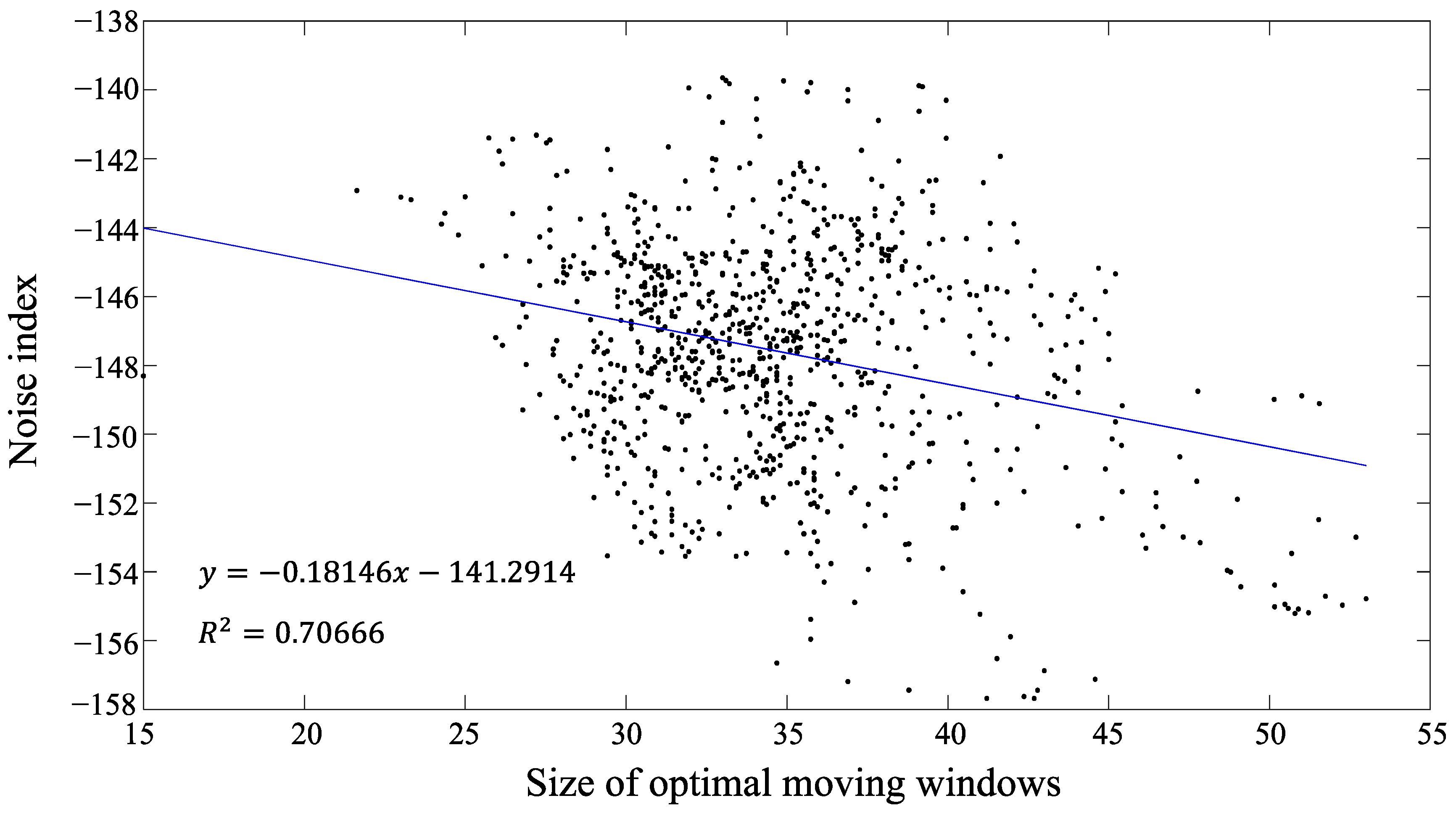
Figure 4.
The proposed data processing procedure for SeaSonde HF radar to detect the geographic coordinates of vessels includes echo identification, locating the peaks of echo signals, and ship direction detection.
Figure 4.
The proposed data processing procedure for SeaSonde HF radar to detect the geographic coordinates of vessels includes echo identification, locating the peaks of echo signals, and ship direction detection.

Figure 5.
Preprocessing for ROI selection: (a) Raw self-spectrum of the monopole of Habn at 07:59:48 on 29 October 2013; (b) Result of closing operation on Figure 5a; (c) ROI selection from the recognition result of Canny edge detection.
Figure 5.
Preprocessing for ROI selection: (a) Raw self-spectrum of the monopole of Habn at 07:59:48 on 29 October 2013; (b) Result of closing operation on Figure 5a; (c) ROI selection from the recognition result of Canny edge detection.

Figure 6.
Schematic results of each step in the ASI algorithm: (a) An ROI of CSS has a strong echo at zero velocity; (b) DC removal of Figure 6a; (c) Moving average surface of Figure 6b; (d) Residual series; (e) The watershed algorithm divides a suspected ship echo into separate regions; (f) Location of the local peak of each suspected vessel (red circle).

Figure 7.
Test of selecting the best 2D MA filter: (a) Skewness and kurtosis of the histogram of the residual series for various moving window sizes; (b) Slope changes in the skewness curve and the convergence condition setting.
Figure 7.
Test of selecting the best 2D MA filter: (a) Skewness and kurtosis of the histogram of the residual series for various moving window sizes; (b) Slope changes in the skewness curve and the convergence condition setting.

Figure 8.
Schematics of the measured antenna pattern and DOA function: (a) The red and blue lines are two cross-loop antenna patterns; the orange line is the loop 1 pointing angle; (b) DOA function; the green peak point represents the signal source.
Figure 8.
Schematics of the measured antenna pattern and DOA function: (a) The red and blue lines are two cross-loop antenna patterns; the orange line is the loop 1 pointing angle; (b) DOA function; the green peak point represents the signal source.

Figure 9.
Two consecutive detection results using the ASI algorithm; the green arrows are radar signals of ship 1: (a) At 7:59 on 29 October 2013 (UTC); (b) At 8:16 on 29 October 2013 (UTC).
Figure 9.
Two consecutive detection results using the ASI algorithm; the green arrows are radar signals of ship 1: (a) At 7:59 on 29 October 2013 (UTC); (b) At 8:16 on 29 October 2013 (UTC).

Figure 10.
Two consecutive direction-finding results using the MUSIC algorithm; the green dots are the DOAs of ship 1: (a) At 7:59 on 29 October 2013 (UTC); (b) At 8:16 on 29 October 2013 (UTC).
Figure 10.
Two consecutive direction-finding results using the MUSIC algorithm; the green dots are the DOAs of ship 1: (a) At 7:59 on 29 October 2013 (UTC); (b) At 8:16 on 29 October 2013 (UTC).

Figure 11.
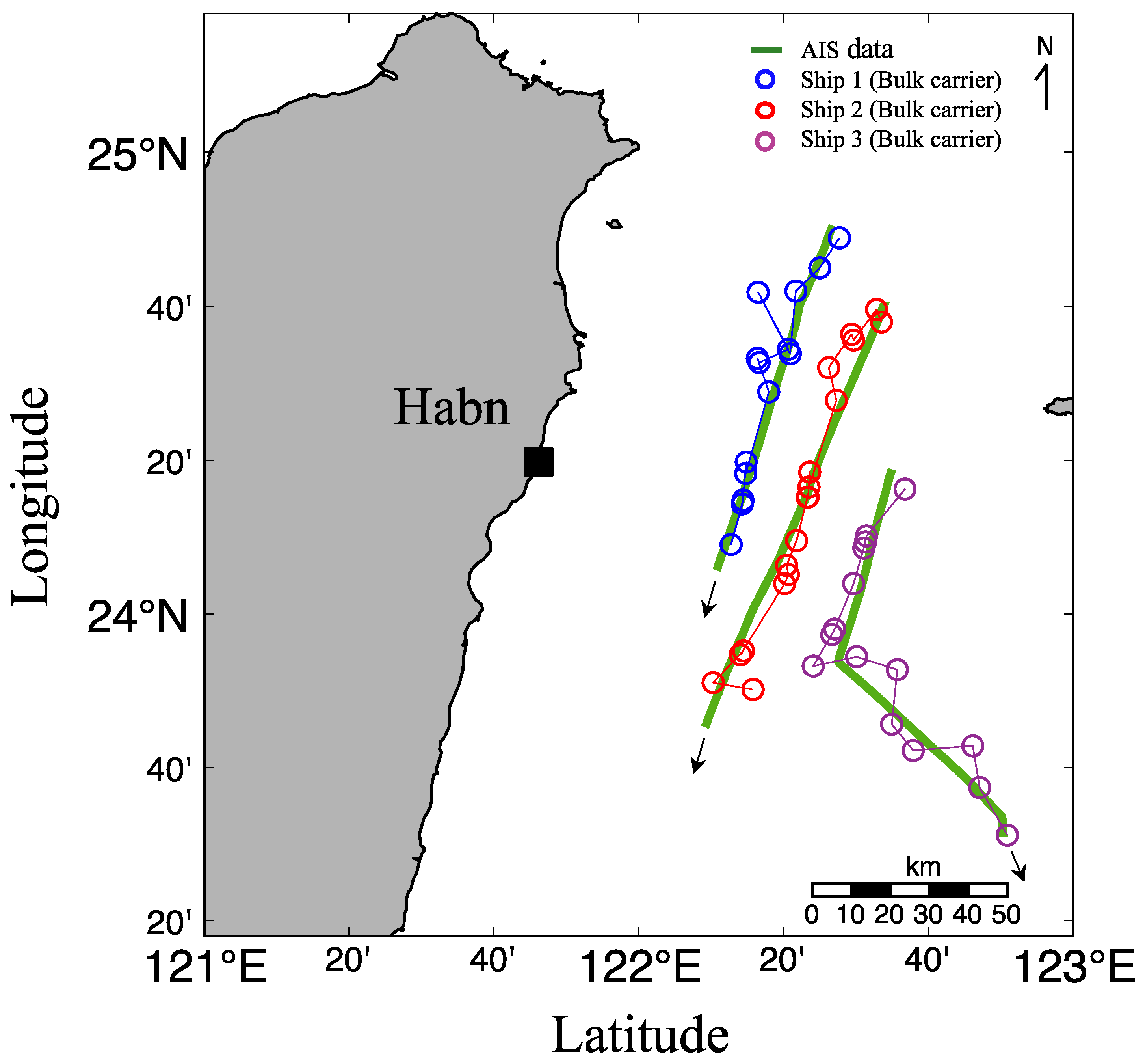
Trajectories of vessels from 29 October 2013 to 31 October 2013; the blue dots are the trajectory predictions of ship 1 at 04:34–09:08 on 29 October 2013; the red dots are those of ship 2 at 00:53–05:43 on 29 October 2013; the purple dots are those of ship 3 at 20:30 on 30 October 2013 to 02:52 on 31 October 2013. The three green lines are the actual tracks from the AIS database.
Figure 11.
Trajectories of vessels from 29 October 2013 to 31 October 2013; the blue dots are the trajectory predictions of ship 1 at 04:34–09:08 on 29 October 2013; the red dots are those of ship 2 at 00:53–05:43 on 29 October 2013; the purple dots are those of ship 3 at 20:30 on 30 October 2013 to 02:52 on 31 October 2013. The three green lines are the actual tracks from the AIS database.

Figure 12.
Scatter plot of the SNR and bearing error statistics of the sample vessels.

Publisher’s Note: MDPI stays neutral with regard to jurisdictional claims in published maps and institutional affiliations. |
© 2021 by the authors. Licensee MDPI, Basel, Switzerland. This article is an open access article distributed under the terms and conditions of the Creative Commons Attribution (CC BY) license (https://creativecommons.org/licenses/by/4.0/).
Share and Cite
MDPI and ACS Style
Chuang, L.Z.-H.; Chen, Y.-R.; Chung, Y.-J. Applying an Adaptive Signal Identification Method to Improve Vessel Echo Detection and Tracking for SeaSonde HF Radar. Remote Sens. 2021, 13, 2453. https://doi.org/10.3390/rs13132453
AMA Style
Chuang LZ-H, Chen Y-R, Chung Y-J. Applying an Adaptive Signal Identification Method to Improve Vessel Echo Detection and Tracking for SeaSonde HF Radar. Remote Sensing. 2021; 13(13):2453. https://doi.org/10.3390/rs13132453
Chicago/Turabian StyleChuang, Laurence Zsu-Hsin, Yu-Ru Chen, and Yu-Jen Chung. 2021. "Applying an Adaptive Signal Identification Method to Improve Vessel Echo Detection and Tracking for SeaSonde HF Radar" Remote Sensing 13, no. 13: 2453. https://doi.org/10.3390/rs13132453
Note that from the first issue of 2016, this journal uses article numbers instead of page numbers. See further details here.