Collision Avoidance of Hexacopter UAV Based on LiDAR Data in Dynamic Environment


1
Department of Military Digital Convergence, Ajou University, Suwon 16499, Korea
2
The 1st R&D Institute, Agency for Defense Development, Daejeon 34186, Korea
*
Author to whom correspondence should be addressed.
Remote Sens. 2020, 12(6), 975; https://doi.org/10.3390/rs12060975
Submission received: 3 March 2020
/
Revised: 12 March 2020
/
Accepted: 13 March 2020
/
Published: 18 March 2020
(This article belongs to the Special Issue Trends in UAV Remote Sensing Applications)
Abstract
:A reactive three-dimensional maneuver strategy for a multirotor Unmanned Aerial Vehicle (UAV) is proposed based on the collision cone approach to avoid potential collision with a single moving obstacle detected by an onboard sensor. A Light Detection And Ranging (LiDAR) system is assumed to be mounted on a hexacopter to obtain the obstacle information from the collected point clouds. The collision cone approach is enhanced to appropriately deal with the moving obstacle with the help of a Kalman filter. The filter estimates the position, velocity, and acceleration of the obstacle by using the LiDAR data as the associated measurement. The obstacle state estimate is utilized to predict the future trajectories of the moving obstacle. The collision detection and obstacle avoidance maneuver decisions are made considering the predicted trajectory of the obstacle. Numerical simulations, including a Monte Carlo campaign, are conducted to verify the performance of the proposed collision avoidance algorithm.
1. Introduction
In the last decade, Unmanned Aerial Vehicles (UAVs) have achieved significant advances in scientific research as well as in real-world applications. Especially, rotary-wing UAVs have been employed for a wide range of application areas due to their vertical takeoff and landing capability. Nowadays, various types of UAVs with different structures keep emerging. For instance, UAVs with six or more rotors have attracted attention due to their higher payload capacity [1,2,3,4,5]. Furthermore, various sensors have been mounted on the UAVs for applications such as autonomous formation flight, surveillance, target tracking, reconnaissance, disaster assistance, etc.
Light Detection And Ranging (LiDAR) is one type of active remote sensing and has been widely employed as a primary ranging device in many autonomous robotic vehicles including UAVs [6,7,8,9,10]. Wallace et al. [11] presented a UAV-borne LiDAR system to collect measurements for forest inventory applications. A Sigma Point Kalman Smoother (SPKS) was applied to combine observations from different sensors. Then, Wallace et al. [12] developed a tree detection algorithm using high-density LiDAR data. The effect of point density on the accuracy of tree detection and delineation was evaluated. On the other hand, Chen et al. [13] integrated LiDAR and UAV to extract detailed surface geologic information. The random sample consensus method was adopted to ascertain the best-fit plane of bedding. Hening et al. [14] presented a data fusion technique for the position and velocity estimation of UAVs. Local position information was provided by a LiDAR sensor, and an adaptive Kalman filter was applied for the integration. Zheng et al. [15] built an obstacle detection system using LiDAR with the consideration of a moving point cloud.
To fully take advantage of UAVs in the real world, a high degree of flight safety related to a close encounter with another UAV should be guaranteed. In a real situation, the obstacle information is unknown prior to deployment and it should be detected by a sensor mounted on the UAV during the mission. The UAV must be capable of avoiding the detected obstacle using the online-collected information. In other words, obstacle detection and avoidance is one of the most important capabilities for the success of UAV applications. Therefore, it is crucial to develop a collision avoidance strategy for the UAV to perform a given mission in a dynamic environment.
Collision avoidance against a moving obstacle has been investigated by various researchers. In the robotics field, Cherubini et al. [16] designed a set of paths during navigation to take into account the obstacle velocity, which was estimated by a Kalman filter. The estimated velocity was used to predict the obstacle’s position within a tentacle-based approach. Ji et al. [17] presented a path planning and tracking framework for autonomous vehicles. The tracking task was formulated as a multiconstrained model predictive control problem, and the front wheel steering angle was calculated to prevent the vehicle from colliding with a moving obstacle. Malone et al. [18] proposed a scheme to incorporate the effect of likely obstacle motion into the desired path of a robot. The method combined an artificial potential field with stochastic reachable set for online path planning. Li et al. [19] developed a controller based on a nonlinear model predictive control for obstacle avoidance. A moving trend function was constructed to predict dynamic obstacle position variances in the prediction horizon. Zhang et al. [20] focused on the tracking of an object in the presence of multiple dynamic obstacles. A method based on conservation of energy was proposed to adjust the motion states of the robot manipulators.
On the other hand, in the aerospace field, Mujumdar and Padhi [21] developed nonlinear geometric guidance and differential geometric guidance, based on aiming point guidance. The guidance law of the UAV was made applicable for moving obstacles by incorporating the Point of Closest Approach (PCA). Wang and Xin [22] addressed the formation control problem where other UAVs are treated as moving obstacles. A nonquadratic avoidance cost function was constructed by an inverse optimal control approach so that the optimal control law was obtained in an analytical form. Yang et al. [23] designed a switching controller to achieve a spatial collision avoidance strategy for fixed-wing UAV. The UAV maintained a safe distance from an intruder by keeping the desired relative bearing and elevation during a collision course. Gageik et al. [24] demonstrated an autonomous flight with low-cost sensors. The movement of an obstacle was handled by the parametrization of the weighted filter. Radmanesh and Kumar [25] formulated a mixed-integer linear program for the path planning problem by incorporating the collision avoidance requirements as the constraints. The constraint relations enforced the formation to visit waypoints and to avoid collision with any intruder aircraft. Lin and Saripalli [26] proposed a sampling-based path planning method based on the Closed-Loop Rapidly-Exploring Random Tree (CL-RRT) algorithm. Using the reachable set, the candidate trajectory method was made robust against unexpected obstacle maneuvers. Santos et al. [27] presented a trajectory tracking controller based on a time-variant artificial potential field with hierarchical objectives using a behavior-based approach. Obstacle motion was taken into account through the variations of the potential function. Marchidan and Bakolas [28] utilized a parameterized vector field that was generated from the decomposition of agent kinematics into normal and tangential components. With a parametric proximity-based eigenvalue function, the agent’s maneuver could be adjusted with little computation effort.
The capability of hovering over a designated position is the unique property of the rotary-wing UAVs enabling various useful applications. For example, with the development of communication techniques, UAV Base Station (UAV-BS) becomes a promising approach to provide wireless connectivity to ground user equipment or other aerial nodes [29,30,31,32]. Moreover, UAV-BS can be utilized in enhancing the coverage and rate performance of the wireless communication networks in scenarios such as an emergency situation. As a base station, it is important for the UAV to perform station keeping at its current location to serve the incoming flow. That is, the performance of the UAV-BS depends on the UAV’s flight time. In this time period, the UAV also estimates the network state and feeds this information to a central agent. Considering its deployment to dangerous sites as a first responder service, the airborne base station should remain intact even in the environment where the presence of an unknown dynamic obstacle is highly likely. Therefore, it is necessary to develop a collision avoidance algorithm which is appropriate during the hovering maneuver of the UAV.
In this study, an enhanced collision avoidance algorithm based on the collision cone approach [33,34] is proposed to deal with a three-dimensional dynamic environment. A hexacopter is considered as the flying platform [35]. The UAV is equipped with a Global Positioning System (GPS) and Attitude and Heading Reference System (AHRS) so that the position and attitude information can be obtained. A conventional Proportional-Derivative (PD) control system is designed to enable waypoint guidance where position and yaw angle commands are fed from the proposed collision avoidance algorithm. An obstacle is completely unknown to the hexacopter initially, and it is detected by a LiDAR system during the flight. From a practical standpoint, the LiDAR has limited Field-of-View (FoV) and sensing range. The obtained obstacle data points are utilized to form a spherical bounding box and collision cone. Also, they are used in an estimator to obtain the state of the obstacle. A discrete-time Kalman filter is adopted with its measurement being the center of the bounding box [36]. The obstacle state estimate is utilized to check the collision condition. The predicted trajectory of the obstacle is considered to detect collision. If a potential collision is detected, the state estimate is used to generate aiming point candidates for the avoidance maneuver. The proposed algorithm removes the candidate points that overlap with the predicted path of the obstacle. This enables the hexacopter to consider the kinematics of the obstacle in choosing the direction of the avoidance maneuver. The point closest to the current velocity of the UAV is chosen as the final aiming point. Numerical simulations are performed to demonstrate the performance of the proposed collision avoidance algorithm. As the previous collision cone approach [37] utilizes the velocity vector of the UAV, its application during the hovering maneuver is difficult, as the velocity is nearly a zero vector. However, the proposed algorithm works well in this situation due to the usage of the relative geometry. That is, the proposed algorithm appropriately handles the avoidance against the moving obstacle, in contrast to the previous algorithm. In addition, a Monte Carlo simulation is performed to verify the robustness of the proposed algorithm.
The remainder of this paper is organized as follows. Section 2 describes the dynamics, control system, and data acquisition system of a hexacopter. The background of the collision cone approach is briefly explained in Section 3. In Section 4, the structure of a discrete-time Kalman filter is presented for the estimation. Then, the collision avoidance algorithm for a moving obstacle is proposed in Section 5. The simulation results are presented in Section 6, and the conclusion is given in Section 7.
2. UAV System
2.1. Dynamics
A hexacopter is configured with six rotors, where three rotors rotate in clockwise direction and the others rotate in counterclockwise direction. A platform of the Tarot 680 hexacopter is shown in Figure 1 as an example. A North-East-Down (NED) coordinate system is considered in an inertial frame. Note that flat-Earth and rigid body are assumed in this study. A body-fixed coordinate system is defined with its origin at the hexacopter’s center of mass and its axes (, , and ) are aligned with the reference direction vector, as shown in Figure 1.
The rigid hexacopter dynamics is governed by the following translational and rotational differential equations [35].
where is the position vector of the hexacopter represented in the NED coordinate system; and are the velocity vector and the angular velocity of the hexacopter represented in the body-fixed coordinate system, respectively; m and are the mass and inertia matrix of the hexacopter, respectively; is the external force of the hexacopter represented in the body-fixed coordinate system; is the external moment of the hexacopter represented in the body-fixed coordinate system; is the gravity vector represented in the NED coordinate system; and () is the direction cosine matrix performing coordinate transformation from the NED coordinate system to the body-fixed coordinate system, which is defined with a (3-2-1) Euler sequence as follows,
where Euler angle is defined between the NED and body-fixed coordinate systems.
The external force and moment of the hexacopter can be expressed as follows.
Then, and have the following relationship with the angular velocity of the rotor,
where and are the thrust and drag coefficients of the rotor, respectively; l is the distance from the hexacopter’s center of mass to the rotor; and is the angular velocity of the i-th rotor with .
2.2. Control Design
In this study, a PD controller is designed to track the desired position vector (, , and ) and yaw angle (). First, the collective thrust command, T, is computed to handle the desired altitude of the hexacopter, which is represented by .
where and are design parameters. The horizontal position controller equations are given as
where and are design parameters. Now, the desired roll and pitch angles, and , respectively, can be obtained as follows.
Then, the commanded roll, pitch, and yaw moments, L, M, and N, respectively, can be computed for the attitude loop as follows,
where , , , , , and are design parameters. Finally, the angular velocities of the six rotors are allocated by using Equation (6) with T, L, M, and N obtained in Equations (7), (13)–(15), respectively. Note that , , , and are delivered from the proposed collision avoidance guidance system described in Section 5.
2.3. LiDAR Data Sensing
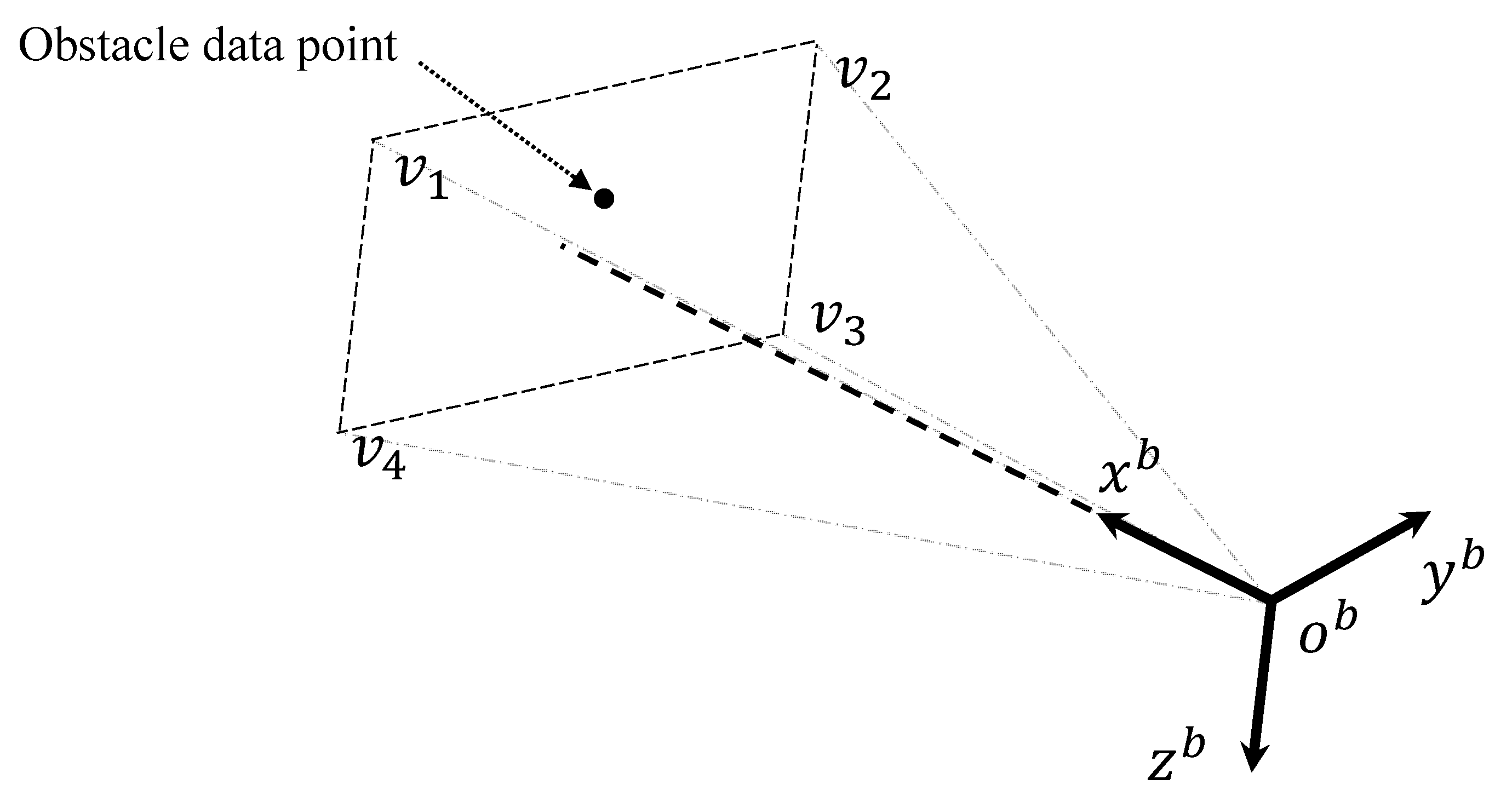
Let us assume that an obstacle consists of a point cloud that represents its external surface. The LiDAR with limited FoV is mounted on the hexacopter and directed along the -axis to acquire obstacle data. The visibility of the obstacle point by the LiDAR can be determined by examining whether the obstacle data point is inside a rectangular pyramid whose vertices are , , , , and , as shown in Figure 2. , , , and in the body-fixed coordinate system can be obtained as follows.
where and are the horizontal and vertical FoV of the LiDAR, respectively, and is a sensing range of the LiDAR. The hexacopter performs its mission with constant obstacle data acquisition from the LiDAR.
3. Review of Basic Collision Cone Approach
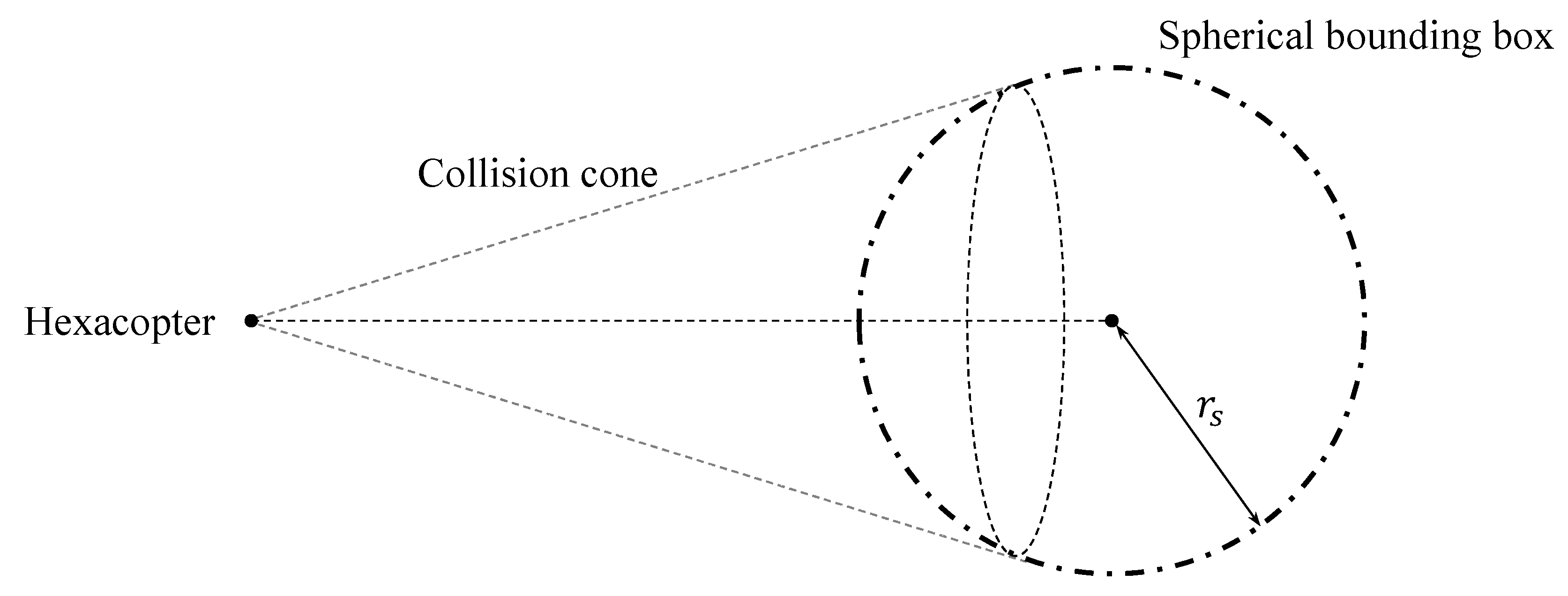
In this study, the collision cone method is adopted as the basis of the collision detection and avoidance logic [33,34]. Let us assume that data points are accumulated by the LiDAR, and that the position vector of the k-th obstacle data point in the NED coordinate system is defined as . Among data points, there are two points associated with the longest pairwise Euclidean distance. Let us define these points as and . Then, the center of a spherical bounding box can be obtained as follows.
Also, the radius of the bounding box can be designed as follows,
where is a safety margin. Finally, a collision cone can be constructed with a set of tangent lines from the hexacopter to the bounding box, as shown in Figure 3.
If the velocity vector of the hexacopter is contained within the collision cone, the detected obstacle is a potential threat to the UAV unless it changes its trajectory. In this case, the hexacopter should perform a collision avoidance maneuver. During the collision avoidance maneuver, the hexacopter is guided to an aiming point instead of the predefined goal point. The aiming point is selected from the points on the intersection curve of the bounding box and the collision cone. In this study, the point closest to the velocity vector of the hexacopter is chosen as the aiming point to minimize the UAV’s maneuver. If the velocity vector of the hexacopter is outside the collision cone, then the UAV is guided to the original goal point. This logic is repeated until the hexacopter reaches the goal point.
4. Obstacle State Estimator
As a moving obstacle is considered in this study, its state should be estimated to implement the proposed collision avoidance algorithm described in Section 5. A discrete-time Kalman filter is constructed for the estimation [36]. First, the filter state is defined as follows,
where , , and are the position, velocity, and acceleration estimates of the obstacle, respectively, represented in the NED coordinate system. Now, the discrete-time state equation for the estimator can be expressed as follows,
where is the sampling time of LiDAR data acquisition, and is a process noise characterized by . On the other hand, the position vector of the center of the bounding box obtained in Equation (17) by the LiDAR system is used as a measurement. Therefore, the measurement equation can be constructed as follows,
where is a measurement noise. In this study, an unknown obstacle is detected by LiDAR sensor that has a limited sensing range. The bounding box enclosing the set of detected data points gradually grows in its size as more of the obstacle comes within the sensing range. In this case, , computed in Equation (17), may differ from the actual center of the obstacle. This error can be treated as a measurement noise, , in the observation model. Finally, using Equations (20) and (21), the discrete-time Kalman filter can be implemented to estimate the state of the obstacle.
The Kalman filter is initiated when the obstacle is detected by the LiDAR for the first time. Then, it is updated at every with newly measured . If cannot be found at a certain step, then virtual measurement, , is modeled to keep the estimator running. This situation may occur when the UAV completely avoids the obstacle and every obstacle data point is out of the LiDAR’s sensing range. The virtual measurement, , is modeled with the state estimate at the previous step as follows.
When the obstacle is detected again, is discarded and the Kalman filter operates with the normal measurement.
5. Collision Avoidance Strategy Against Moving Obstacle
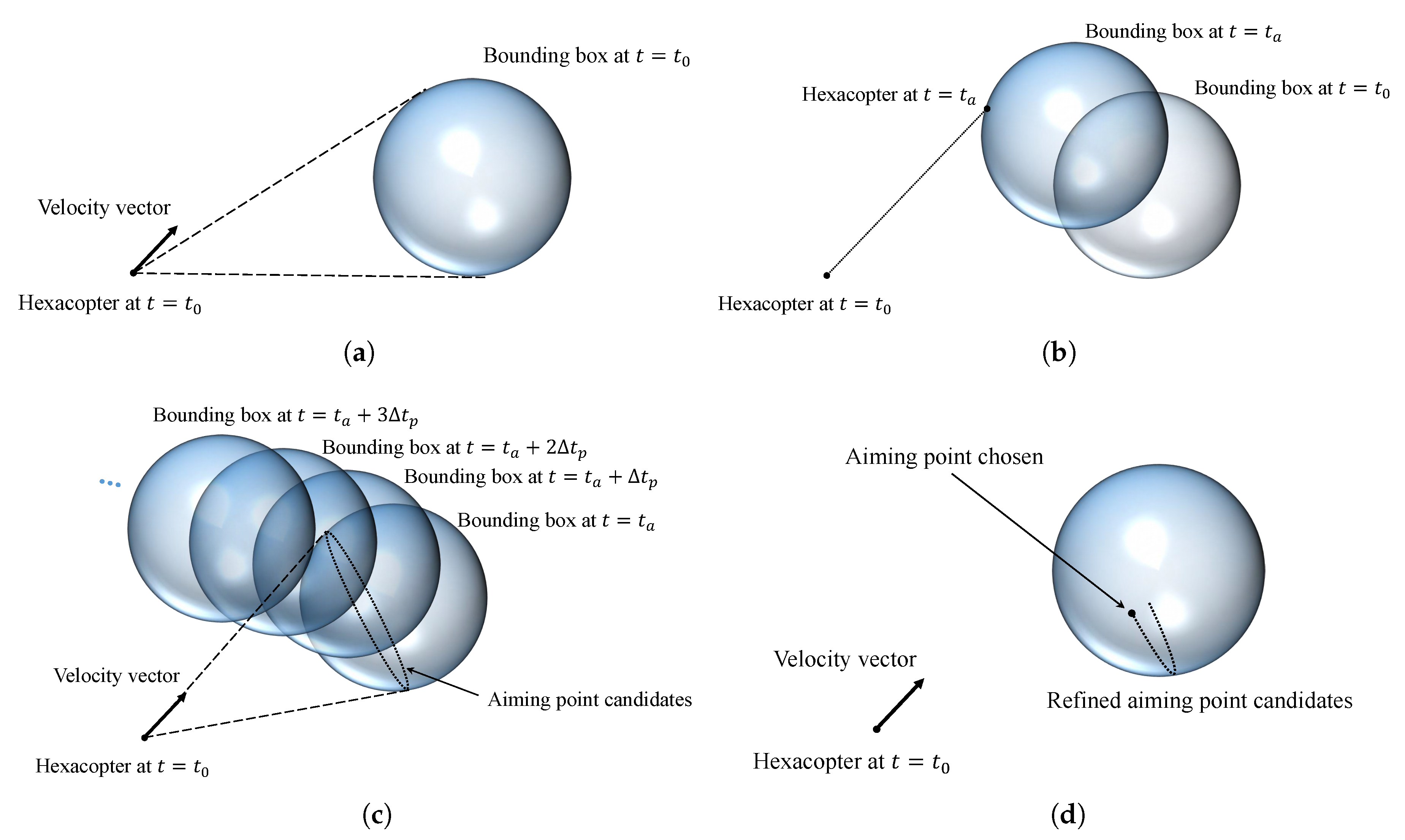
As the Kalman filter provides the obstacle information, these state estimates are utilized in the collision detection algorithm and avoidance law considering the dynamic environment. The proposed strategy proceeds in several stages as shown in Figure 4.
Although an obstacle is within the range of the LiDAR, the velocity vector of the hexacopter is outside the collision cone at , as shown in Figure 4a. Then, the previous approach determines that the UAV is not on a collision course to the obstacle and allows the UAV to continue flying toward the goal point, as it only incorporates the current position and velocity in collision detection. On the contrary, the method proposed in this study utilizes the instantaneous short-term predictions for the obstacle trajectory to determine whether the UAV is on the course to close proximity of the obstacle. The trajectory of the obstacle is predicted by utilizing the state estimate as
with the prediction horizon, , of various lengths. Also, the future position of the hexacopter can be predicted as follows,
where is the velocity vector of the hexacopter represented in the NED coordinate system. Note that the acceleration vector is not used in Equation (24) because the abrupt change in the acceleration by the proposed algorithm may result in poor prediction. If the Euclidean distance between the predicted obstacle position, , and the predicted UAV position, , is smaller than the bounding sphere radius, , at a certain , the UAV determines that it is on a collision course. Let us define this moment as , as shown in Figure 4b. Additionally, note that is constantly calculated using Equation (18) whenever the obstacle is detected by the LiDAR and the algorithm keeps updating the maximum observed value for safety reasons, yet this approach might be conservative. The hexacopter is inside the spherical bounding box of the obstacle in Figure 4b, which means a collision.
Now, a collision avoidance maneuver is required. To perform the avoidance maneuver, the collision cone is constructed with the bounding box at and the position of the UAV at , as shown in Figure 4c. The aiming point for the UAV chosen in the direction of the obstacle’s future trajectory is likely to increase the chance of a close encounter with the obstacle at the next time step, which is disadvantageous from the viewpoint of minimizing the probability of a possible collision. An additional pruning process is therefore conducted after creating the aiming point candidates to prevent undesirable and ineffective collision avoidance maneuver due to a wrong choice of aiming point. The trace of bounding boxes starting from can be created as shown in Figure 4c with the prediction horizon given by . These boxes can then be used to trim the candidate points. If an aiming point candidate is inside the predicted envelope of the bounding boxes at any moment, then that point is eliminated from the candidate set.
Some candidate points may be removed by the pruning process as shown in Figure 4d. Then, the final aiming point is chosen from the remaining candidate points. Even though the point closest to the velocity vector of the hexacopter is chosen, the chosen point may be far from the velocity vector because of the elimination step, as shown in Figure 4d.
The aiming point provided as the final result of the collision avoidance strategy comprises the desired position part of the guidance command. Meanwhile, the desired yaw angle is designed so that the LiDAR faces toward the center of the spherical bounding box.
The reasoning behind the yaw angle command design is to keep the obstacle inside of the LiDAR’s FoV for the consecutive state estimation.
The overall flowchart of the proposed collision avoidance algorithm is shown in Figure 5.
6. Numerical Simulation
Numerical simulations are conducted to demonstrate the performance of the proposed collision avoidance algorithm. The parameters of the hexacopter dynamics and control system, estimator, and collision avoidance used in the numerical simulation are listed in Table 1.
The time step for numerical integration and control update is 0.01 s, whereas the sampling time of the LiDAR data acquisition, , is set to 0.1 s. The slower rate for the LiDAR measurement update is due to the large amount of computational effort required to process the point cloud data in each cycle. Not only the obstacle state estimator, but also the collision avoidance guidance algorithm, is triggered by the arrival of new LiDAR data. Consequently, they have the same update rate of 10Hz, and the UAV’s autopilot utilizes the latest updated command.
For the control system of the hexacopter, and in Equations (11) and (12) are limited in the range of ±20° to avoid excessive maneuver. Meanwhile, in Table 1 is the covariance of the initial estimation error of , where diag refers to a square matrix with the elements inside the square bracket being the diagonal entries. As an obstacle is completely unknown initially, there is no choice but to set as a zero vector. Additionally, the Kalman filter takes time for the state estimate to converge to a steady-state value. Therefore, the proposed collision avoidance algorithm begins to incorporate the obstacle state estimate a few time steps after the first detection of the obstacle in order to allow a period for the filter state to converge. In this study, (5 steps) is chosen as this period.
For every simulation in this section, the initial position of the hexacopter is set to in the NED coordinate system. Also, the initial velocity, angular velocity, and Euler angle of the hexacopter are set to zero.
6.1. Simulation I: Hovering Situation
In Simulation I, the hovering situation is considered, which is the case where the goal point is given by the initial position of the UAV. Namely, the hexacopter stays at if a detected obstacle is not considered as a potential threat. An obstacle whose shape is a sphere with the radius of 1 m is considered. Its initial position is set to with a constant velocity of so that it is on a collision course.
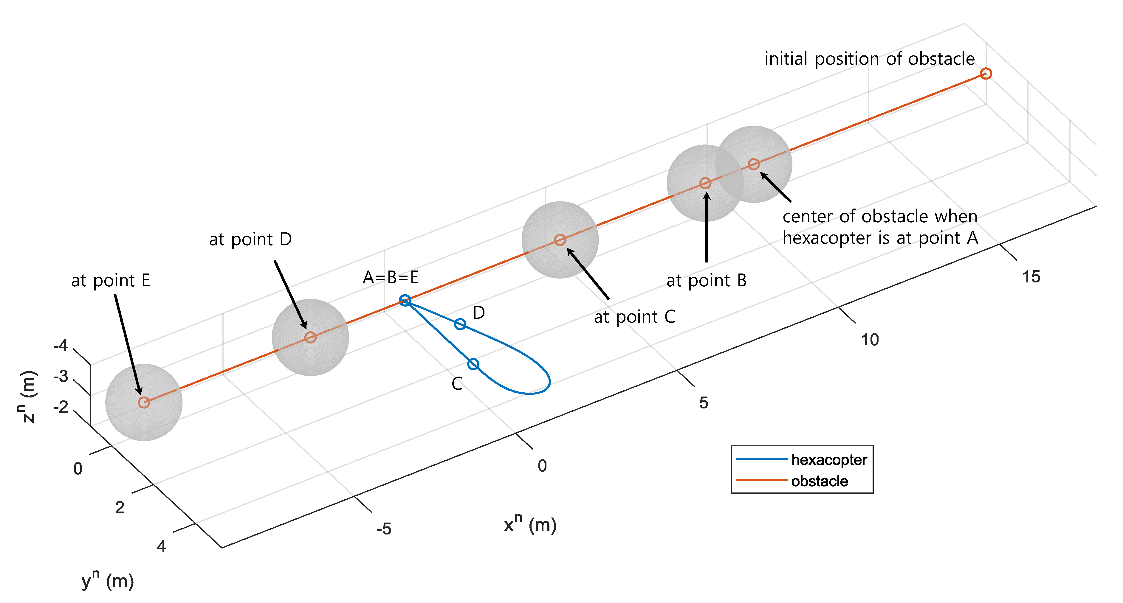
Figure 6 shows the trajectories of the hexacopter and the obstacle in the NED coordinate system.
Additionally, Figure 7 shows the time responses of the attitude, angular velocity, velocity, and absolute velocity of the hexacopter, and the minimum distance between the UAV and the obstacle. Also, Figure 8 shows the time responses of the estimated state along with the true state plotted as a reference of comparison. Note that all state estimates are set to zero at initial state.
Initially ( s), the obstacle is outside the sensing range of the LiDAR, because is set to 10 m in Table 1. Then, the obstacle is first detected by the hexacopter at point A ( s), as shown in Figure 7c. However, the UAV does not immediately perform avoidance maneuver, but simply continues hovering. This is because the collision avoidance algorithm incorporates the estimated obstacle information only after the filter transients are died out, as explained above. Moreover, only a small part of the obstacle enters the range of the LiDAR at point A. The computed at point A is , whereas its true state is . This difference may result in a poor estimation. As shown in Figure 8, the state estimates are still at initial zero values at point A. However, after s, which is denoted as point B, most of the state estimates are converged to the true states and these are used in the collision avoidance algorithm. Now, the hexacopter predicts the trajectory of the obstacle, and determines that it is on a collision course.
At point B ( s), the hexacopter triggers the collision avoidance maneuver by guiding to the aiming point, instead of the goal point. At the same time, the yaw angle command is generated to direct toward so that the detected obstacle remains inside the LiDAR’s FoV, as shown in Figure 7a. At point C ( s), the UAV determines that the future position of the obstacle does not collide with it. That is, the hexacopter is outside of the predicted bounding boxes of the obstacle. Although the UAV heads back to the goal point from this moment, it produces the different trajectory compared to the past one as shown in Figure 6. This is due to the control system of the hexacopter, which generates the change of in advance of , as shown in Figure 7a. Simultaneously, -axis of the hexacopter is aligned with the goal point by adjusting .
At point D ( s), the hexacopter reaches the minimum distance of m as shown in Figure 7c. However, considering the direction of the obstacle’s velocity vector, it is no longer a threat to the UAV. Finally, at point E ( s), the hexacopter reaches the goal point as shown in Figure 6 and is able to perform hovering maneuver again.
In the hovering situation, the velocity vector of the hexacopter is a zero vector, which means that it is difficult to utilize the previous collision cone approach [37]. On the contrary, the proposed algorithm gives consideration to the relative motion as it uses the obstacle information estimated by the Kalman filter. Therefore, the proposed algorithm can be adopted while the UAV is in the hovering state.
6.2. Simulation II: Waypoint Guidance
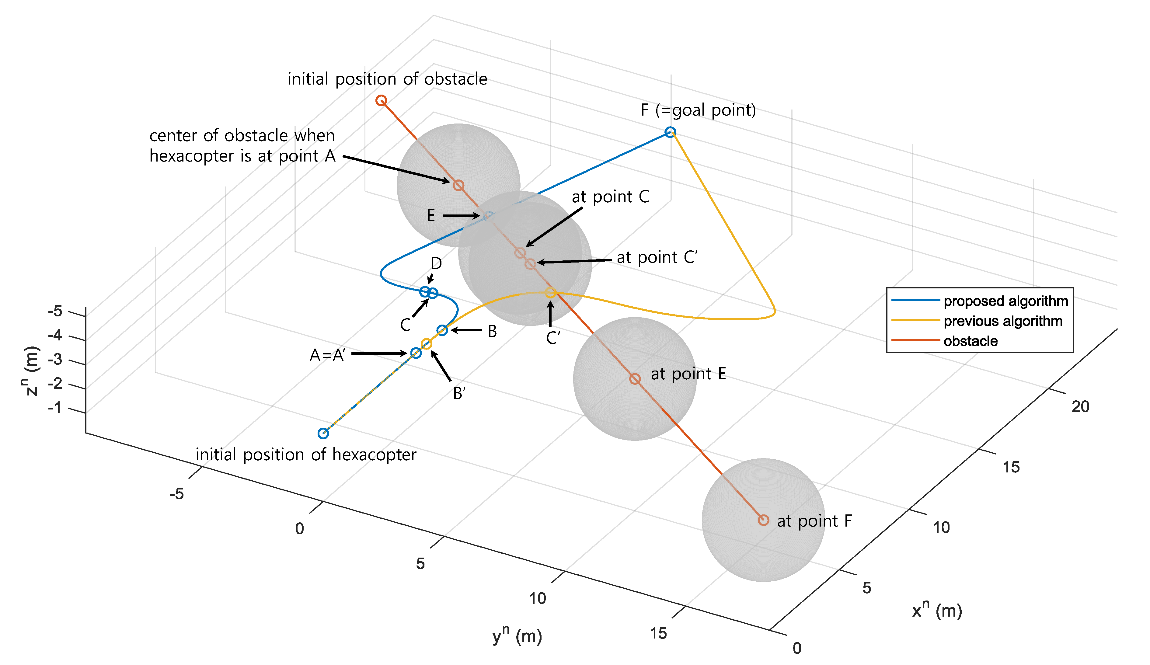
In Simulation II, the proposed collision avoidance algorithm is compared to the previous algorithm [37]. The goal point is set to , and the hexacopter initially heads for the goal point. A sphere with a radius of m is initially located at and flies toward the path of the UAV. The magnitudes of the velocity vector and the acceleration vector are m/s and m/s2, respectively. Also, their unit vector is .
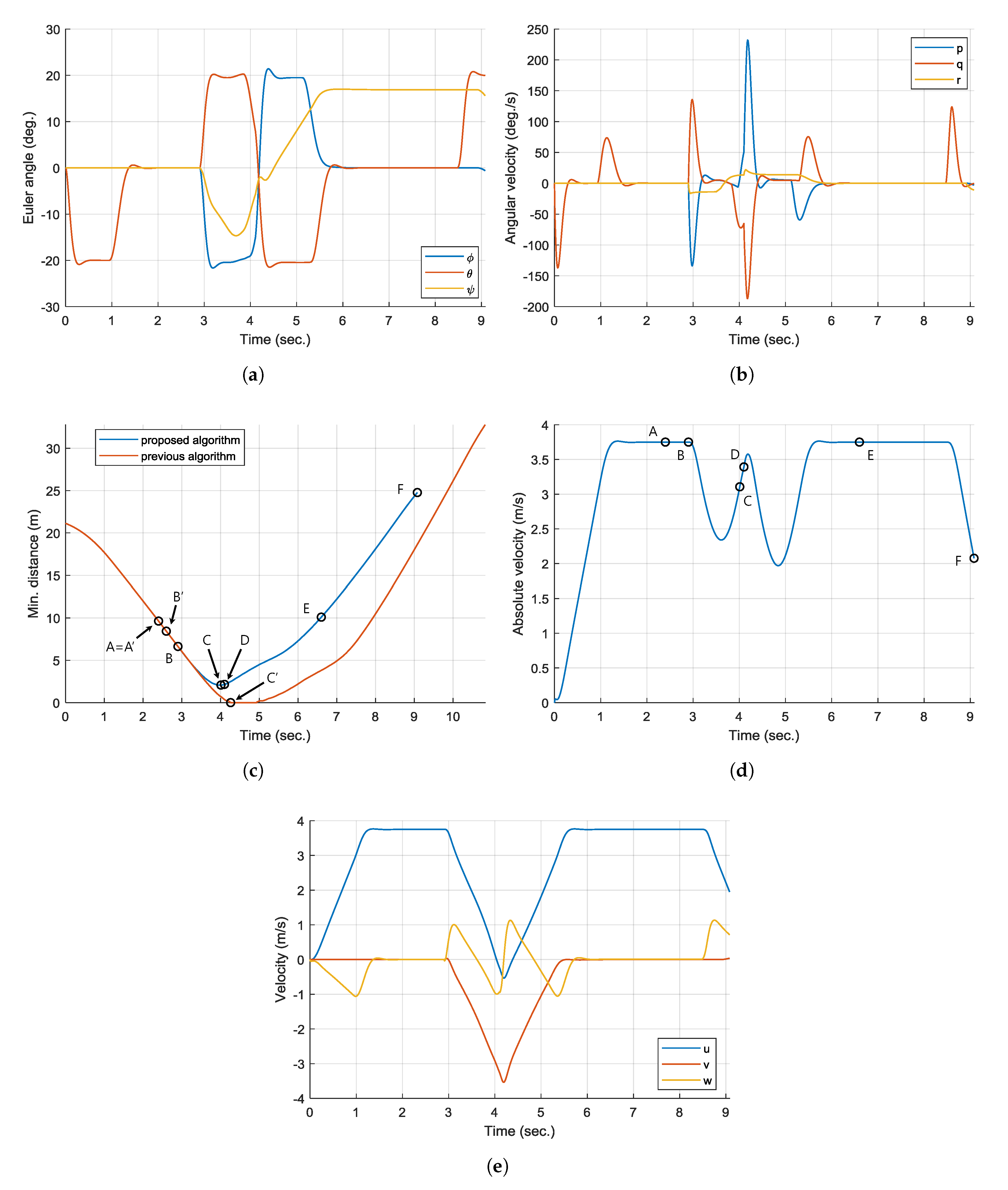
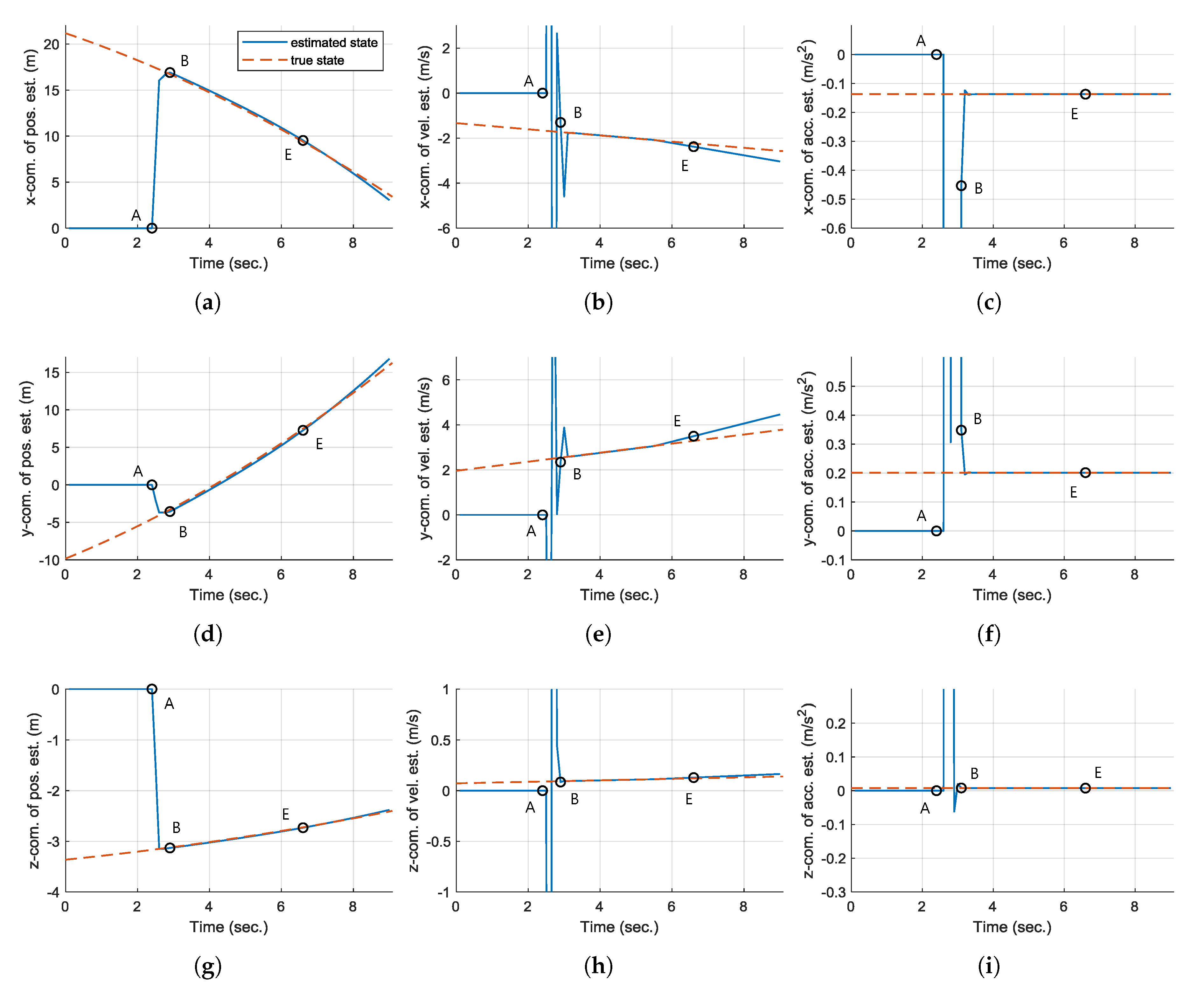
Figure 9 shows the trajectories of the hexacopter with the proposed algorithm and the previous algorithm, and the obstacle in the NED coordinate system. Also, Figure 10 shows the time responses of the attitude, angular velocity, velocity, and absolute velocity of the hexacopter, and the minimum distance between the UAV and the obstacle. Figure 11 shows the time responses of the state estimate of the Kalman filter.
The obstacle enters the range and FoV of the LiDAR at point A (= point A’, s) for both the proposed and previous algorithms, as shown in Figure 9 and Figure 10c. Then, the hexacopter with the proposed algorithm starts collision avoidance maneuver at point B ( s), as the UAV collides with one of the predicted bounding boxes. As shown in Figure 11, the state estimates show sufficient convergence to the true states from point B, which are appropriate to be utilized in the collision avoidance algorithm. On the other hand, the hexacopter with the previous algorithm triggers the avoidance maneuver at point B’ ( s), which is earlier than the one with the proposed algorithm. This is because the previous algorithm does not utilize the obstacle state estimator. As soon as the computed collision cone includes the velocity vector of the UAV, the UAV heads for the aiming point as shown in Figure 9.
The difference can be witnessed from this moment. As a benefit of incorporating the pruning step in the aiming point processing pipeline, the proposed algorithm selects the aiming point on the opposite side of the obstacle’s predicted trajectory. However, the previous algorithm chooses the aiming point without considering the short-term future movement of the obstacle. As a consequence, the UAV cannot withstand the acceleration and the velocity of the obstacle and eventually collides with it at point C’ ( s), as shown in Figure 9. Note that the minimum distance between the UAV and the obstacle is 0 m at point C’ in Figure 10c. That is, although the previous algorithm shows earlier transition to the collision avoidance mode than the proposed algorithm, it fails to avoid the moving obstacle.
On the contrary, the UAV with the proposed algorithm successfully avoids the obstacle and reaches the minimum distance of m at point C ( s) as shown in Figure 10c. This is a reasonable value, considering that is set to 2 m in Table 1. At point D ( s), the hexacopter determines that the obstacle is no longer a threat, and switches to the goal point guidance. Note that there is a time lag between point C and point D due to the sampling time of the LiDAR, .
At point E ( s), the obstacle deviates from the sensing range of the LiDAR, as shown in Figure 10c, and cannot be obtained from this point. Then, the virtual measurement, , is calculated using Equation (22) to produce the measurement of Equation (21) for the Kalman filter. However, the deviation from the true state can be observed before point E, especially in Figure 11b,e. This is because of the incorrect calculation of with partial detection of the obstacle. Nevertheless, the goal point guidance is maintained. Finally, the UAV reaches the point F ( s) as shown in Figure 9.
6.3. Simulation III: Monte Carlo Simulation
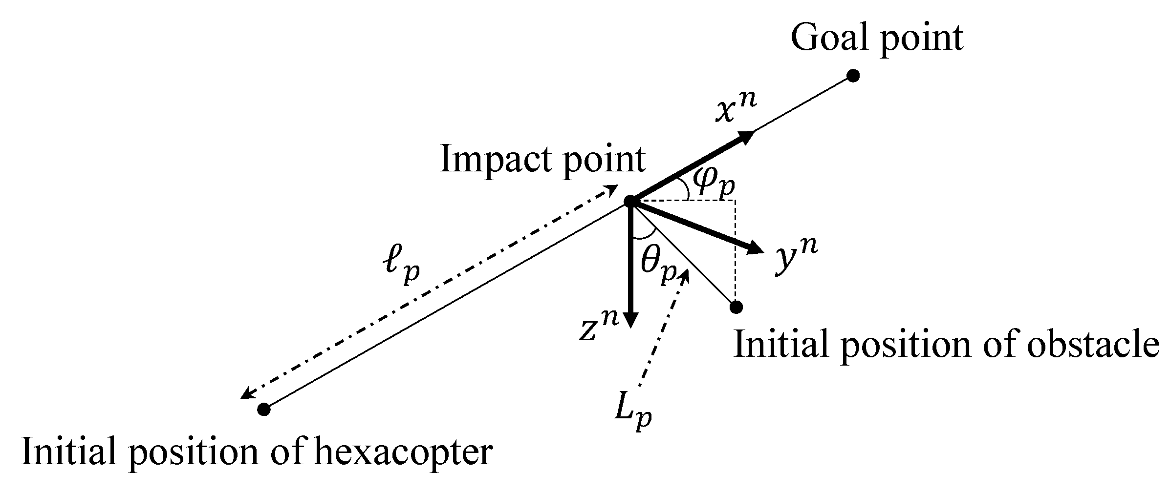
A Monte Carlo simulation is carried out to investigate the robustness of the proposed algorithm. Five-hundred different scenarios are generated, where the following properties of the obstacle are assigned using a continuous uniform distribution: impact point, initial position, radius, velocity, and acceleration. First, the impact point with the UAV is randomly chosen between the initial position of the hexacopter, , and the goal point, , as shown in Figure 12.
Let us define this impact point as where is shown in Figure 12. Then, the time-to-go of the UAV to the point can be calculated as follows,
where is the average speed of the hexacopter. Referring to Figure 7d and Figure 10d, is roughly chosen as m/s. Note that the generated cases with s are excluded, considering a reasonable initial gap between the UAV and the obstacle. Then, the ranges of the magnitude of the acceleration and the velocity are set to and , respectively. If these are denoted as and , the length between and the initial position of the obstacle can be computed as follows.
Now, and in Figure 12 are randomly chosen from and , respectively, which determine the impact angle. The initial position of the obstacle, , can be obtained as follows.
Also, the acceleration, , and the velocity, , of the obstacle can be computed as follows.
Finally, the radius of the obstacle is chosen in the range of . Note that the cases with the obstacle approaching from the direction outside the FoV of the LiDAR are also excluded from the result.
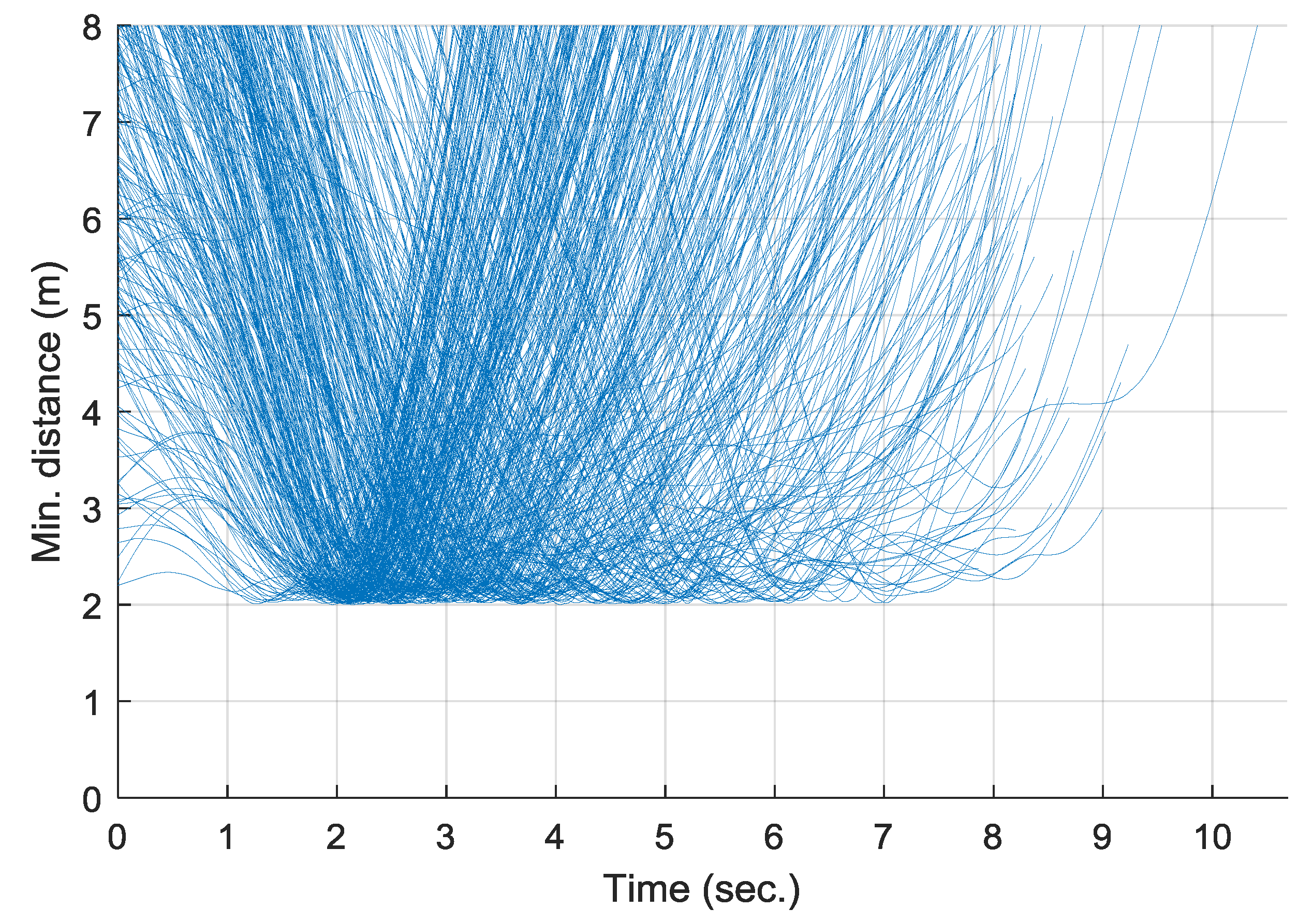
The Monte Carlo simulation result is shown in Figure 13, which is the time responses of the minimum distance between the hexacopter and the obstacle for each case. In every case, the hexacopter reaches the goal point without violating the safety requirement, as the minimum separation is greater than the added safety margin, , at all times. The Monte Carlo simulation result confirms the successful collision avoidance performance of the proposed algorithm.
7. Conclusions
In this study, a collision avoidance algorithm of a hexacopter UAV is proposed. The algorithm is based on the collision cone approach, and is improved to handle a moving obstacle by considering the short-term predictions for the obstacle trajectory with the aid of an obstacle state estimator. A PD controller is used to generate angular velocities of the rotors where the command is fed from the proposed guidance algorithm. A LiDAR system on the UAV obtains the obstacle data points to form the spherical bounding box around the detected region of the obstacle and also the collision cone. Sometimes, the LiDAR system may lose the obstacle due to its limited sensing range and FoV. In this case, the Kalman filter produces a virtual measurement with the previous state estimate. A collision is detected by examining the predicted position of both the UAV and the obstacle. The obstacle state estimate also contributes to an avoidance maneuver of UAV by removing the points that are unreasonable to be taken as candidates of the aiming point. The numerical simulation results, including a Monte Carlo campaign, are shown to verify the proposed guidance algorithm. The results demonstrate that the hexacopter properly handles the moving obstacle; unlike the previous method that does not explicitly consider the predicted relative movement. For future research, the proposed algorithm will be extended to deal with multiple obstacles. An appropriate decision-making algorithm should be developed to assess the obstacles in terms of the level of threat.
Author Contributions
Conceptualization, J.P.; methodology, J.P. and N.C.; validation, N.C.; investigation, J.P. and N.C.; resources, J.P.; writing—original draft preparation, J.P.; writing—review and editing, N.C.; visualization, J.P. and N.C.; supervision, N.C.; funding acquisition, J.P. All authors have read and agreed to the published version of the manuscript.
Funding
This work was supported by the new faculty research fund of Ajou University.
Conflicts of Interest
The authors declare no conflicts of interest.
References
- Omari, S.; Hua, M.; Ducard, G.; Hamel, T. Hardware and Software Architecture for Nonlinear Control of Multirotor Helicopters. IEEE/ASME Trans. Mech. 2013, 18, 1724–1736. [Google Scholar] [CrossRef] [Green Version]
- Giribet, J.I.; Sanchez-Pena, R.S.; Ghersin, A.S. Analysis and Design of a Tilted Rotor Hexacopter for Fault Tolerance. IEEE Trans. Aerosp. Electron. Syst. 2016, 52, 1555–1567. [Google Scholar] [CrossRef]
- Lee, H.; Kim, H.; Kim, H.J. Planning and Control for Collision-Free Cooperative Aerial Transportation. IEEE Trans. Autom. Sci. Eng. 2018, 15, 189–201. [Google Scholar] [CrossRef]
- Zhang, J.; Gu, D.; Deng, C.; Wen, B. Robust and Adaptive Backstepping Control for Hexacopter UAVs. IEEE Access 2019, 7, 163502–163514. [Google Scholar] [CrossRef]
- Chen, Y.; Zhang, G.; Zhuang, Y.; Hu, H. Autonomous Flight Control for Multi-Rotor UAVs Flying at Low Altitude. IEEE Access 2019, 7, 42614–42625. [Google Scholar] [CrossRef]
- Li, Z.; Tan, J.; Liu, H. Rigorous Boresight Self-Calibration of Mobile and UAV LiDAR Scanning Systems by Strip Adjustment. Remote Sens. 2019, 11, 442. [Google Scholar] [CrossRef] [Green Version]
- Lei, L.; Qiu, C.; Li, Z.; Han, D.; Han, L.; Zhu, Y.; Wu, J.; Xu, B.; Feng, H.; Yang, H.; et al. Effect of Leaf Occlusion on Leaf Area Index Inversion of Maize Using UAV–LiDAR Data. Remote Sens. 2019, 11, 1067. [Google Scholar] [CrossRef] [Green Version]
- Yang, Q.; Su, Y.; Jin, S.; Kelly, M.; Hu, T.; Ma, Q.; Li, Y.; Song, S.; Zhang, J.; Xu, G.; et al. The Influence of Vegetation Characteristics on Individual Tree Segmentation Methods with Airborne LiDAR Data. Remote Sens. 2019, 11, 2880. [Google Scholar] [CrossRef] [Green Version]
- Lin, Y.C.; Cheng, Y.T.; Zhou, T.; Ravi, R.; Hasheminasab, S.M.; Flatt, J.E.; Troy, C.; Habib, A. Evaluation of UAV LiDAR for Mapping Coastal Environments. Remote Sens. 2019, 11, 2893. [Google Scholar] [CrossRef] [Green Version]
- Yan, W.; Guan, H.; Cao, L.; Yu, Y.; Li, C.; Lu, J. A Self-Adaptive Mean Shift Tree-Segmentation Method Using UAV LiDAR Data. Remote Sens. 2020, 12, 515. [Google Scholar] [CrossRef] [Green Version]
- Wallace, L.; Lucieer, A.; Watson, C.; Turner, D. Development of a UAV-LiDAR System with Application to Forest Inventory. Remote Sens. 2012, 4, 1519–1543. [Google Scholar] [CrossRef] [Green Version]
- Wallace, L.; Lucieer, A.; Watson, C.S. Evaluating Tree Detection and Segmentation Routines on Very High Resolution UAV LiDAR Data. IEEE Trans. Geosci. Remote Sens. 2014, 52, 7619–7628. [Google Scholar] [CrossRef]
- Chen, N.; Ni, N.; Kapp, P.; Chen, J.; Xiao, A.; Li, H. Structural Analysis of the Hero Range in the Qaidam Basin, Northwestern China, Using Integrated UAV, Terrestrial LiDAR, Landsat 8, and 3-D Seismic Data. IEEE J. Sel. Top. Appl. Earth Observ. Remote Sens. 2015, 8, 4581–4591. [Google Scholar] [CrossRef]
- Hening, S.; Ippolito, C.; Krishnakumar, K. 3D LiDAR SLAM Integration with GPS/INS for UAVs in Urban GPS-Degraded Environments. In Proceedings of the AIAA Infotech@Aerospace Conference, Grapevine, TX, USA, 9–13 January 2017. [Google Scholar]
- Zheng, L.; Zhang, P.; Tan, J.; Li, F. The Obstacle Detection Method of UAV Based on 2D Lidar. IEEE Access 2019, 7, 163437–163448. [Google Scholar] [CrossRef]
- Cherubini, A.; Spindler, F.; Chaumette, F. Autonomous Visual Navigation and Laser-Based Moving Obstacle Avoidance. IEEE Trans. Intell. Transp. Syst. 2014, 15, 2101–2110. [Google Scholar] [CrossRef]
- Ji, J.; Khajepour, A.; Melek, W.W.; Huang, Y. Path Planning and Tracking for Vehicle Collision Avoidance Based on Model Predictive Control With Multiconstraints. IEEE Trans. Veh. Technol. 2017, 66, 952–964. [Google Scholar] [CrossRef]
- Malone, N.; Chiang, H.; Lesser, K.; Oishi, M.; Tapia, L. Hybrid Dynamic Moving Obstacle Avoidance Using a Stochastic Reachable Set-Based Potential Field. IEEE Trans. Robot. 2017, 33, 1124–1138. [Google Scholar] [CrossRef]
- Li, S.; Li, Z.; Yu, Z.; Zhang, B.; Zhang, N. Dynamic Trajectory Planning and Tracking for Autonomous Vehicle With Obstacle Avoidance Based on Model Predictive Control. IEEE Access 2019, 7, 132074–132086. [Google Scholar] [CrossRef]
- Zhang, H.; Jin, H.; Liu, Z.; Liu, Y.; Zhu, Y.; Zhao, J. Real-Time Kinematic Control for Redundant Manipulators in a Time-Varying Environment: Multiple-Dynamic Obstacle Avoidance and Fast Tracking of a Moving Object. IEEE Trans. Ind. Inform. 2020, 16, 28–41. [Google Scholar] [CrossRef]
- Mujumdar, A.; Padhi, R. Reactive Collision Avoidance Using Nonlinear Geometric and Differential Geometric Guidance. J. Guid. Control Dyn. 2011, 34, 303–310. [Google Scholar] [CrossRef]
- Wang, J.; Xin, M. Integrated Optimal Formation Control of Multiple Unmanned Aerial Vehicles. IEEE Trans. Control Syst. Technol. 2013, 21, 1731–1744. [Google Scholar] [CrossRef]
- Yang, X.; Alvarez, L.M.; Bruggemann, T. A 3D Collision Avoidance Strategy for UAVs in a Non-Cooperative Environment. J. Intell. Robot. Syst. 2013, 70, 315–327. [Google Scholar] [CrossRef] [Green Version]
- Gageik, N.; Benz, P.; Montenegro, S. Obstacle Detection and Collision Avoidance for a UAV With Complementary Low-Cost Sensors. IEEE Access 2015, 3, 599–609. [Google Scholar] [CrossRef]
- Radmanesh, M.; Kumar, M. Flight Formation of UAVs in Presence of Moving Obstacles Using Fast-Dynamic Mixed Integer Linear Programming. Aerosp. Sci. Technol. 2016, 50, 149–160. [Google Scholar] [CrossRef] [Green Version]
- Lin, Y.; Saripalli, S. Sampling-Based Path Planning for UAV Collision Avoidance. IEEE Trans. Intell. Transp. Syst. 2017, 18, 3179–3192. [Google Scholar] [CrossRef]
- Santos, M.C.P.; Rosales, C.D.; Sarcinelli-Filho, M.; Carelli, R. A Novel Null-Space-Based UAV Trajectory Tracking Controller With Collision Avoidance. IEEE/ASME Trans. Mech. 2017, 22, 2543–2553. [Google Scholar] [CrossRef]
- Marchidan, A.; Bakolas, E. Collision Avoidance for an Unmanned Aerial Vehicle in the Presence of Static and Moving Obstacles. J. Guid. Control Dyn. 2020, 43, 96–110. [Google Scholar] [CrossRef]
- Al-Hourani, A.; Kandeepan, S.; Lardner, S. Optimal LAP Altitude for Maximum Coverage. IEEE Wirel. Commun. Lett. 2014, 3, 569–572. [Google Scholar] [CrossRef] [Green Version]
- Mozaffari, M.; Saad, W.; Bennis, M.; Debbah, M. Efficient Deployment of Multiple Unmanned Aerial Vehicles for Optimal Wireless Coverage. IEEE Commun. Lett. 2016, 20, 1647–1650. [Google Scholar] [CrossRef]
- Mozaffari, M.; Saad, W.; Bennis, M.; Debbah, M. Wireless Communication Using Unmanned Aerial Vehicles (UAVs): Optimal Transport Theory for Hover Time Optimization. IEEE Trans. Wirel. Commun. 2017, 16, 8052–8066. [Google Scholar] [CrossRef]
- Saxena, V.; Jaldén, J.; Klessig, H. Optimal UAV Base Station Trajectories Using Flow-Level Models for Reinforcement Learning. IEEE Trans. Cogn. Commun. Netw. 2019, 4, 1101–1112. [Google Scholar] [CrossRef]
- Chakravarthy, A.; Ghose, D. Obstacle Avoidance in a Dynamic Environment: A Collision Cone Approach. IEEE Trans. Syst. Man Cybern. Part A Syst. Hum. 1998, 28, 562–574. [Google Scholar] [CrossRef] [Green Version]
- Chakravarthy, A.; Ghose, D. Generalization of the Collision Cone Approach for Motion Safety in 3-D Environments. Autonomous Robots 2012, 32, 243–266. [Google Scholar] [CrossRef]
- Stevens, B.L.; Lewis, F.L. Aircraft Control and Simulation; Wiley: Hoboken, NJ, USA, 2003; pp. 1–481. [Google Scholar]
- Simon, D. Optimal State Estimation: Kalman, H Infinity, and Nonlinear Approaches; John Wiley & Sons: Hoboken, NJ, USA, 2006; pp. 123–129. [Google Scholar]
- Park, J.; Kim, Y. Collision Avoidance for Quadrotor Using Stereo Vision Depth Maps. IEEE Trans. Aerosp. Electron. Syst. 2015, 51, 3226–3241. [Google Scholar] [CrossRef]
Figure 1.
Tarot 680 hexacopter platform and its coordinate systems.
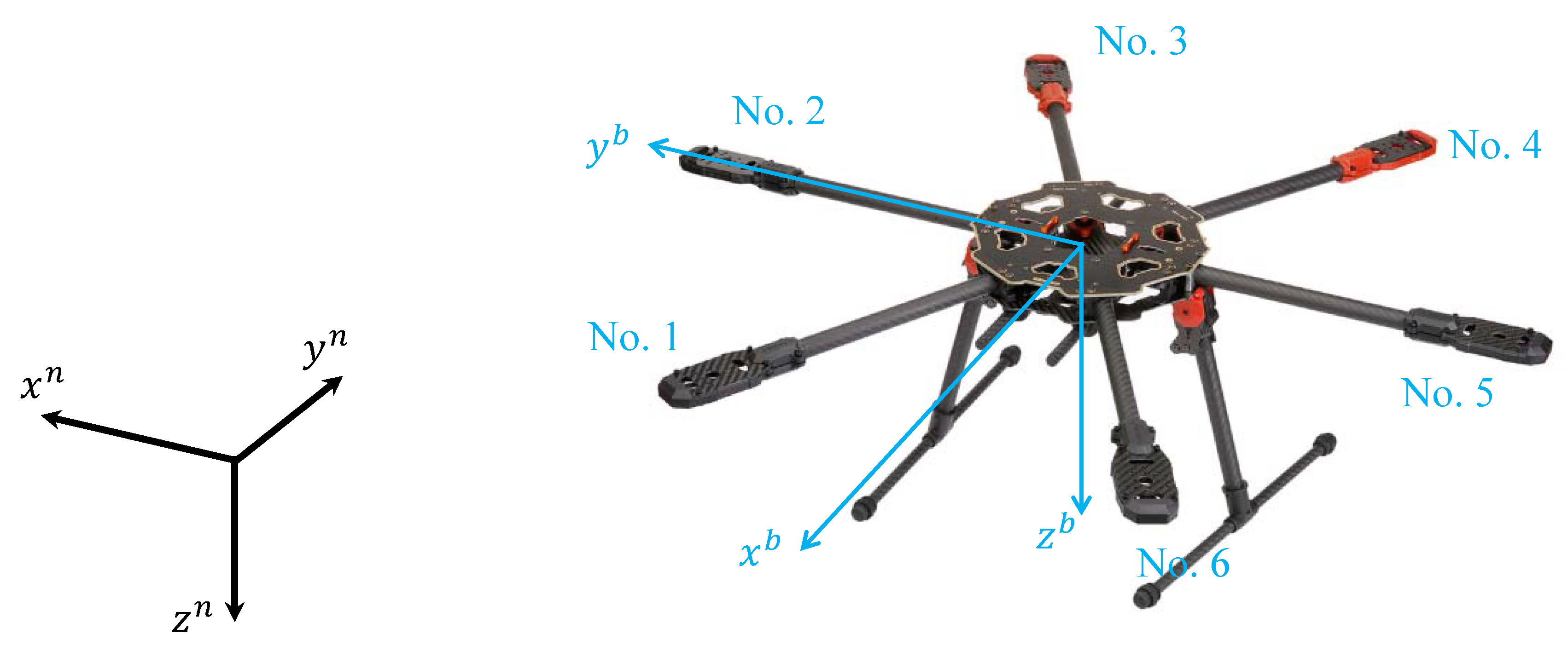
Figure 2.
Obstacle data acquisition with Light Detection And Ranging (LiDAR).

Figure 3.
Constructed bounding box and collision cone.

Figure 4.
Collision avoidance strategy using predicted trajectory of obstacle: (a) velocity vector outside the collision cone at , (b) collision at , (c) pruning process, and (d) final aiming point candidates.
Figure 4.
Collision avoidance strategy using predicted trajectory of obstacle: (a) velocity vector outside the collision cone at , (b) collision at , (c) pruning process, and (d) final aiming point candidates.

Figure 5.
Flowchart of the proposed collision avoidance process.
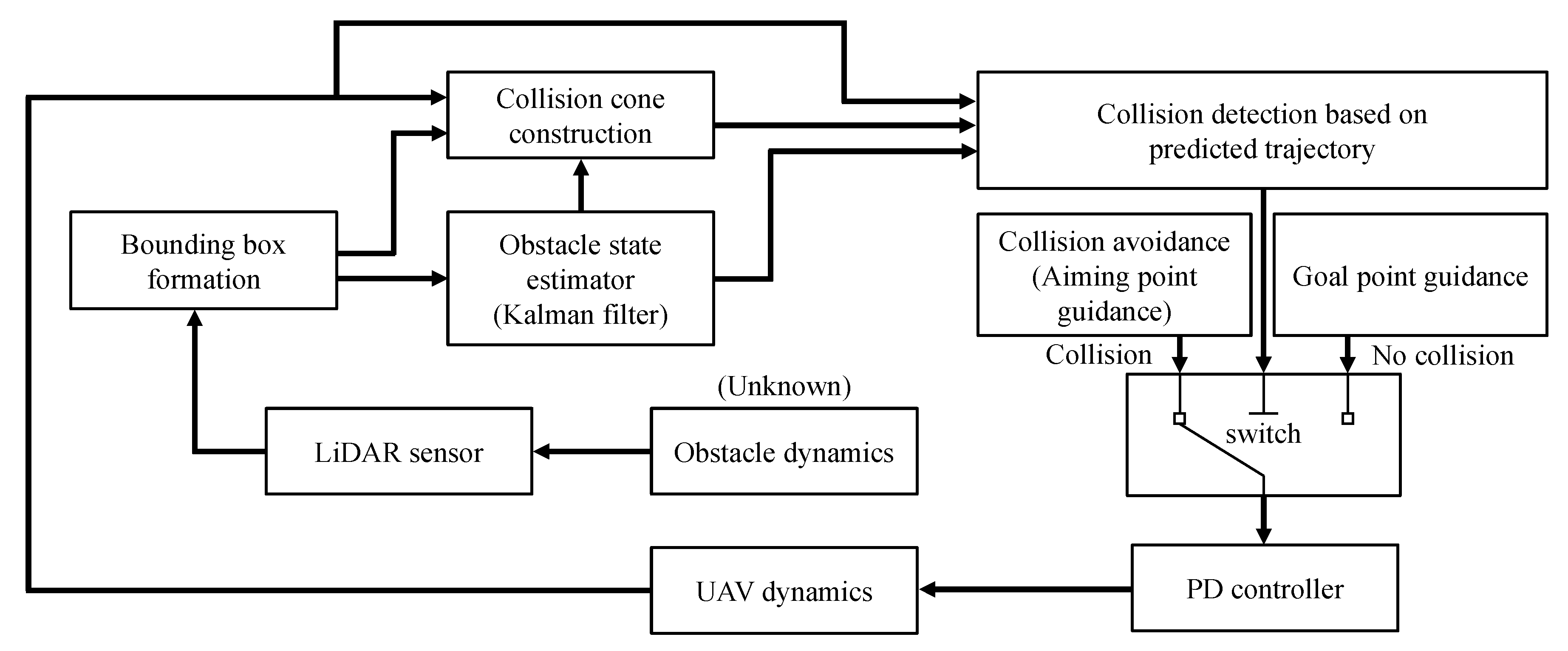
Figure 6.
Trajectories of the hexacopter and the obstacle (azimuth: −33°, elevation: 37°, Simulation I).
Figure 6.
Trajectories of the hexacopter and the obstacle (azimuth: −33°, elevation: 37°, Simulation I).

Figure 7.
Time histories of UAV-related variables (Simulation I): (a) attitude, (b) body rate, (c) minimum distance between UAV and obstacle, (d) absolute velocity, and (e) velocity (body-fixed coordinate system).
Figure 7.
Time histories of UAV-related variables (Simulation I): (a) attitude, (b) body rate, (c) minimum distance between UAV and obstacle, (d) absolute velocity, and (e) velocity (body-fixed coordinate system).
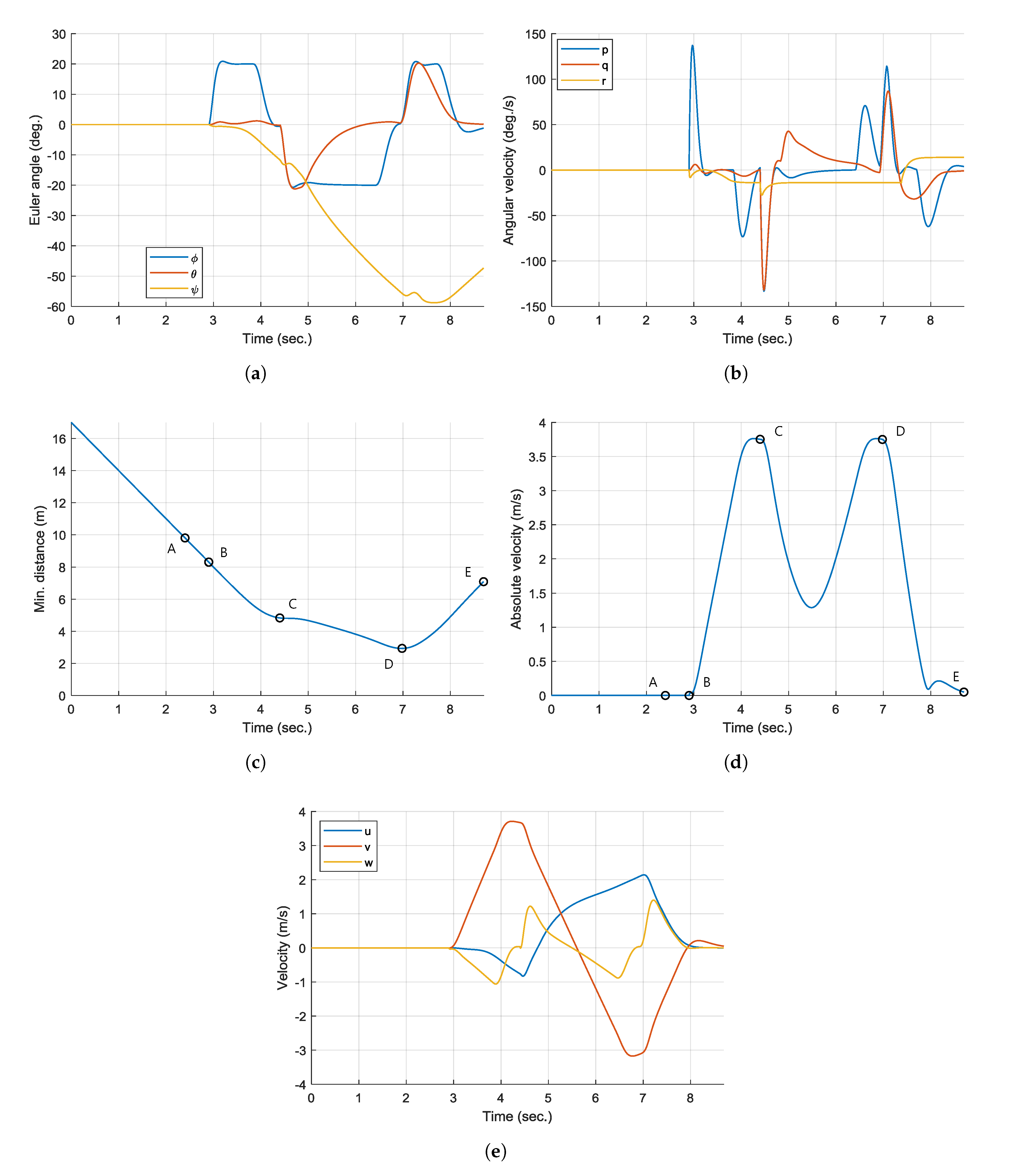
Figure 8.
Time histories of the state estimate (Simulation I): (a) , (b) , (c) , (d) , (e) , (f) , (g) , (h) , and (i) .
Figure 8.
Time histories of the state estimate (Simulation I): (a) , (b) , (c) , (d) , (e) , (f) , (g) , (h) , and (i) .
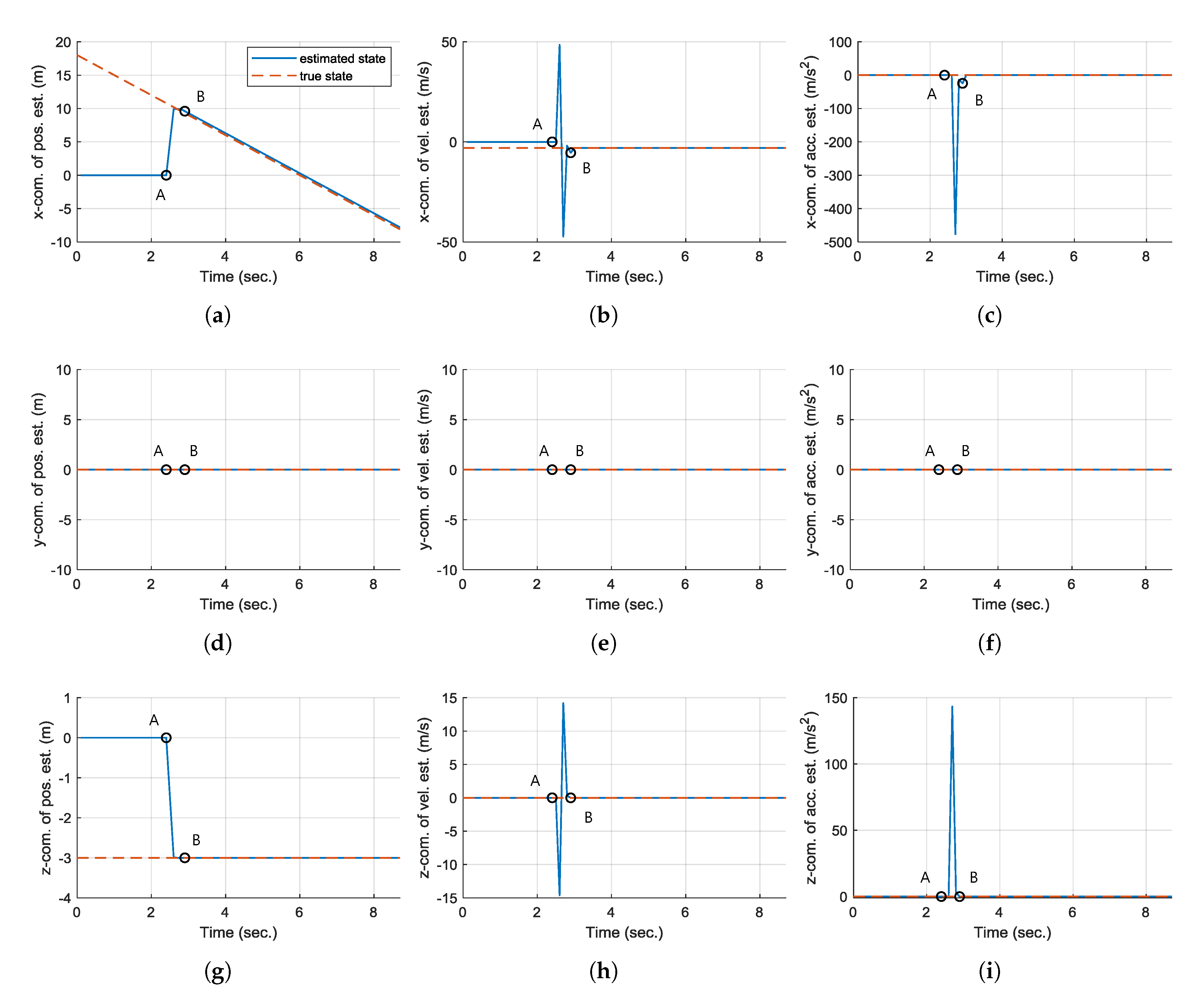
Figure 9.
Trajectories of the hexacopter and the obstacle (azimuth: −60°, elevation: 30°, Simulation II).
Figure 9.
Trajectories of the hexacopter and the obstacle (azimuth: −60°, elevation: 30°, Simulation II).

Figure 10.
Time histories of UAV-related variables (Simulation II): (a) attitude, (b) body rate, (c) minimum distance between UAV and obstacle, (d) absolute velocity, and (e) velocity (body-fixed coordinate system).
Figure 10.
Time histories of UAV-related variables (Simulation II): (a) attitude, (b) body rate, (c) minimum distance between UAV and obstacle, (d) absolute velocity, and (e) velocity (body-fixed coordinate system).

Figure 11.
Time histories of the state estimate (Simulation II): (a) , (b) , (c) , (d) , (e) , (f) , (g) , (h) , and (i) .
Figure 11.
Time histories of the state estimate (Simulation II): (a) , (b) , (c) , (d) , (e) , (f) , (g) , (h) , and (i) .

Figure 12.
Generating obstacle properties for Monte Carlo simulation (Simulation III).

Figure 13.
Time history of minimum distance between UAV and obstacle (Simulation III).


Table 1.
Parameters of the hexacopter, Kalman filter, and collision avoidance used in numerical simulation.
Table 1.
Parameters of the hexacopter, Kalman filter, and collision avoidance used in numerical simulation.
| Hexacopter dynamics | |||||||
| m | 2.356 kg | kg m2 | kg m2 | kg m2 | |||
| l | 0.5 m | Ns2 | Ns2 m | g | 9.8 m/s2 | ||
| Hexacopter controller | |||||||
| 3 rad/s2 | 0.8 | 3 rad/s2 | 0.8 | ||||
| 15 rad/s2 | 0.7 | 15 rad/s2 | 0.7 | ||||
| 5 rad/s2 | 0.9 | ||||||
| LiDAR sensor | |||||||
| 0.1 s | 10 m | 170° | 30° | ||||
| Kalman filter | |||||||
| diag | |||||||
| diag | |||||||
| diag | |||||||
| Collision avoidance | |||||||
| 2 m | Max. | 30 s | 0.1 s | ||||
© 2020 by the authors. Licensee MDPI, Basel, Switzerland. This article is an open access article distributed under the terms and conditions of the Creative Commons Attribution (CC BY) license (http://creativecommons.org/licenses/by/4.0/).
Share and Cite
MDPI and ACS Style
Park, J.; Cho, N. Collision Avoidance of Hexacopter UAV Based on LiDAR Data in Dynamic Environment. Remote Sens. 2020, 12, 975. https://doi.org/10.3390/rs12060975
AMA Style
Park J, Cho N. Collision Avoidance of Hexacopter UAV Based on LiDAR Data in Dynamic Environment. Remote Sensing. 2020; 12(6):975. https://doi.org/10.3390/rs12060975
Chicago/Turabian StylePark, Jongho, and Namhoon Cho. 2020. "Collision Avoidance of Hexacopter UAV Based on LiDAR Data in Dynamic Environment" Remote Sensing 12, no. 6: 975. https://doi.org/10.3390/rs12060975
Note that from the first issue of 2016, this journal uses article numbers instead of page numbers. See further details here.