Improving Spatial Agreement in Machine Learning-Based Landslide Susceptibility Mapping
by
 , , , ,
Mohammed Sarfaraz Gani Adnan
1,2,* ,
,
Md Salman Rahman
3 ,
,
Nahian Ahmed
4 ,
,
Bayes Ahmed
5,6 ,
,
Md. Fazleh Rabbi
7 and
Rashedur M. Rahman
4 1
Environmental Change Institute, School of Geography and the Environment, University of Oxford, South Parks Road, Oxford OX13QY, UK
2
Department of Urban and Regional Planning, Chittagong University of Engineering and Technology (CUET), Chittagong 4349, Bangladesh
3
Department of Civil Engineering, Chittagong University of Engineering and Technology (CUET), Chittagong 4349, Bangladesh
4
Department of Electrical and Computer Engineering, North South University, Bashundhara, Dhaka 1229, Bangladesh
5
Institute for Risk and Disaster Reduction (IRDR), University College London (UCL), Gower Street, London WC1E 6BT, UK
6
Department of Disaster Science and Management, Faculty of Earth and Environmental Sciences, University of Dhaka, Dhaka 1000, Bangladesh
7
Department of Geography and Environmental Studies, University of Chittagong, Chittagong 4331, Bangladesh
*
Author to whom correspondence should be addressed.
Remote Sens. 2020, 12(20), 3347; https://doi.org/10.3390/rs12203347
Submission received: 6 September 2020
/
Revised: 28 September 2020
/
Accepted: 12 October 2020
/
Published: 14 October 2020
(This article belongs to the Special Issue Remote Sensing of Natural Hazards)
Abstract
:Despite yielding considerable degrees of accuracy in landslide predictions, the outcomes of different landslide susceptibility models are prone to spatial disagreement; and therefore, uncertainties. Uncertainties in the results of various landslide susceptibility models create challenges in selecting the most suitable method to manage this complex natural phenomenon. This study aimed to propose an approach to reduce uncertainties in landslide prediction, diagnosing spatial agreement in machine learning-based landslide susceptibility maps. It first developed landslide susceptibility maps of Cox’s Bazar district of Bangladesh, applying four machine learning algorithms: K-Nearest Neighbor (KNN), Multi-Layer Perceptron (MLP), Random Forest (RF), and Support Vector Machine (SVM), featuring hyperparameter optimization of 12 landslide conditioning factors. The results of all the four models yielded very high prediction accuracy, with the area under the curve (AUC) values range between 0.93 to 0.96. The assessment of spatial agreement of landslide predictions showed that the pixel-wise correlation coefficients of landslide probability between various models range from 0.69 to 0.85, indicating the uncertainty in predicted landslides by various models, despite their considerable prediction accuracy. The uncertainty was addressed by establishing a Logistic Regression (LR) model, incorporating the binary landslide inventory data as the dependent variable and the results of the four landslide susceptibility models as independent variables. The outcomes indicated that the RF model had the highest influence in predicting the observed landslide locations, followed by the MLP, SVM, and KNN models. Finally, a combined landslide susceptibility map was developed by integrating the results of the four machine learning-based landslide predictions. The combined map resulted in better spatial agreement (correlation coefficients range between 0.88 and 0.92) and greater prediction accuracy (0.97) compared to the individual models. The modelling approach followed in this study would be useful in minimizing uncertainties of various methods and improving landslide predictions.
1. Introduction
Due to the destructive potential of landslides, this natural phenomenon poses a serious threat to human life, property, and the environment in the areas in which they occur [1,2]. Access to continuous and accurate information on landslide occurrence is essential for managing the risk to this unpredictable hazard [2,3]. Mapping landslide susceptibility is a widely conceived approach to estimating the likelihood of occurrence of this complex natural phenomenon [1,3,4,5]. The development of remote sensing technologies in the last few decades enables researchers to map landslide susceptibility more efficiently, due to the availability of high spatial and temporal resolution data [3,4,6]. For instance, high-resolution remote sensing (satellite imagery) data are used to develop various thematic layers explaining the topography, land cover, geology, and hydrology, which are essential parameters for predicting landslides [4,7]. Remote sensing techniques are also useful in developing accurate landslide inventory maps [3,6].
Along with the quality of available data, the choice of appropriate methodology is essential for developing reliable susceptibility maps [2]. During the last several decades, many landslide susceptibility models have been developed based on the geographic information system (GIS) and remote sensing technology [8]. Examples of such models include the weights-of-evidence [9,10], multivariate regression analysis [10,11], analytical hierarchy process [12], and the evidential belief function [13]. Applications of various machine learning algorithms in landslide susceptibility mapping (LSM) have evolved in recent decades. As a widely applicable method in data mining, the K-Nearest Neighbor (KNN) algorithm made early appearances in landslide prediction [14,15]. The Logistic Regression (LR) [2,12] and Support Vector Machine (SVM) [8,16] models also gained much popularity as adaptive systems for LSM [15]. Artificial neural networks in the form of a Multi-Layer Perceptron (MLP) were also used for this task [17]. More recently, evidence from various studies indicates that ensembles such as the Random Forest (RF) model can improve machine learning-based landslide prediction [1,18]. However, the outcomes of landslide susceptibility mapping could be subject to considerable uncertainties due to errors and variability in model choice, data used, system understanding, weighting factors, and human judgment [19,20].
Since the access to accurate landslide prediction maps is the prerequisite to decision-makers, the results must be carefully analyzed and critically reviewed before disseminating to support the end-users [9]. While developing landslide susceptibility maps, challenges may arise in (i) measuring the accuracy of a susceptibility assessment [21], and (ii) selecting an “optimal” combination of methods for susceptibility assessments [22]. Most of the validation processes of LSM consist of two steps: simulating landslide susceptibility and comparing the predicted results with the observed landslide locations [1,9]. Validation techniques must possess qualities such as reliability, robustness, degree of fitting, and prediction skill [21]. However, the performance evaluation of most of the LSMs was carried out based on the testing datasets [9,23]. Thus, a similar performance of multiple models at the testing landslide locations does not ascertain the same degree of agreement in terms of spatial predicted patterns [9].
Whilst many recent studies applied various combinations of machine learning algorithms to map landslide susceptibility [23,24,25,26], pixel-wise agreement in landslide prediction between various methods is inadequately understood. The resultant spatial heterogeneity in landslide prediction with different techniques creates uncertainties in LSM [9,19,27]. To address this challenge, this study aimed to propose a method to reduce uncertainties in landslide prediction. Therefore, it evaluated the extent of agreement of landslide prediction maps generated by applying four different machine learning algorithms. A combined landslide prediction map was developed by integrating the results of these four models. The study was carried out in Cox’s Bazar district of Bangladesh (Figure 1).
2. Materials and Methods
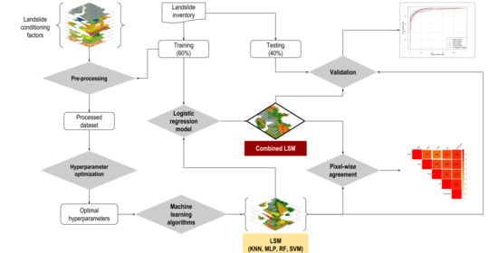
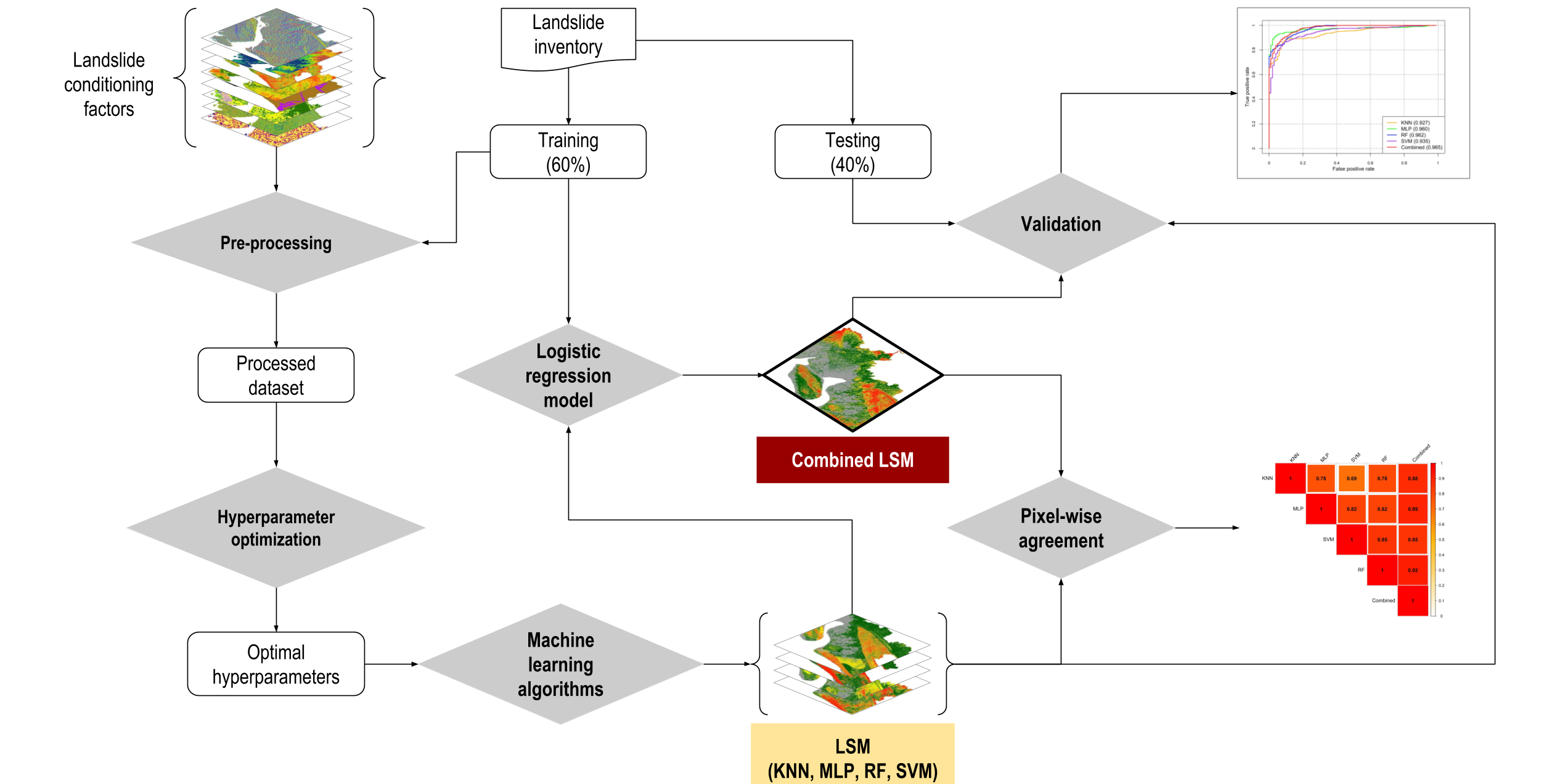
The study was conducted in three stages. First, landslide susceptibility maps (LSMs) of the study area were developed using four machine learning algorithms: K-Nearest Neighbor (KNN), Multi-Layer Perceptron (MLP), Random Forest (RF), and Support Vector Machine (SVM). Second, the extent of spatial agreement of predicted patterns in LSMs was assessed by estimating the pixel-wise correlation of landslide probabilities obtained using various methods. Finally, an LSM was developed combining results from the four machine learning models (Figure 2). This study also estimated population exposure to landslide by overlaying gridded population layers of the year 2020, collected from WorldPop [29] and UNHCR [30], on LSMs.
2.1. Study Area
This study addressed the Cox’s Bazar district, which is located in the south eastern region of Bangladesh (Figure 1a). The study area lies between latitude 20°53′46.7″ N and 21°14′29.8″ N, and longitude 92°02′08.2″ E and 92°18′27.0″ E. It is comprised of seven (out of eight) sub-districts (locally termed as Upazilas) of Cox’s Bazar district (Figure 1b). The low-lying areas such as Kutubdia sub-district, part of Maheshkhali sub-district, and Saint Martin’s island (Figure 1b) were not considered in this study. The study area is diverse and unique, both in terms of ecosystem services and biodiversity, and currently, an epitome of global geopolitics as it is accommodating over one million Rohingya refugees. It is characterized by relatively high elevation land (mean elevation is 18 m), compared to the rest of the country. At present, approximately a total of 3.4 million people inhabit 1869 km2 of land (estimated using data from WorldPop [29] and UNHCR [30]).
The area receives the annual mean precipitation of 4288 mm [31]. The heavy rainfall triggers both flash floods and landslides in this area [11,12]. The majority of the historical landslides in Bangladesh occurred in this region [11]. For instance, a major landslide triggered by heavy rain in June 2017 killed at least 156 people in the south eastern hilly region of Bangladesh where the study area is located [32]. Unplanned urbanization, rapid growth of population, hill cutting, and deforestation are associated with the recent increase in landslide hazards [11,31]. Notably, Rohingya refugee camps, especially the Kutupalong camp of Ukhia sub-district (Figure 3) is located in areas that are highly susceptible to landslides. The Kutupalong camp is considered as the most densely populated refugee settlement area in the world, where around 75,000 people live per km2 [31,33]. Any catastrophic landslide will cause significant damage to human lives and assets. Hence, an accurate assessment of landslide susceptibility is paramount for developing a plan for landslide risk management.
2.2. Landslide Inventory Mapping
Landslide inventory mapping is one of the essential steps for landslide prediction and susceptibility mapping. This study utilized the landslide inventory map developed by Ahmed, Rahman, Sammonds, Islam, and Uddin [11] (Figure 3). They developed the latest landslide inventory map of the Cox’s Bazar district by retrieving the historical landslide information from newspapers and various organizations and later verified those with global positioning system (GPS) and reconnaissance surveys. This study also used information about landslide movement type, its distribution and style, rate of flow, damage, the volume of displacement, material, and the reason for movement by preparing a landslide investigation form collected from Ahmed, Rahman, Sammonds, Islam, and Uddin [11]. A total of 1262 sample locations were used, where the number of landslide and non-landslide locations was 670 and 592, respectively. To develop the models, it is necessary to obtain non-landslide cells (where landslides did not occur). From the existing literature, Huang et al. [34] identified three methods for obtaining non-landslide grid cells: (i) the seed cell procedure; (ii) randomly selecting non-landslide locations from the landslide free areas; and (iii) non-landslide locations selected in areas with a slope lower than 2°. This study followed the second approach to select random locations within the study area, where landslides did not occur. These cells provided the models with the necessary data during the training stage [35,36]. The sample locations were split into two classes: (i) 60% locations (52% landslide and 48% non-landslide locations) were used to train the machine learning-based landslide prediction models, and (ii) 40% testing locations (54% landslide and 46% non-landslide locations) were employed to evaluate the performance of the machine learning models (Figure 2).
2.3. Landslide Conditioning Factor
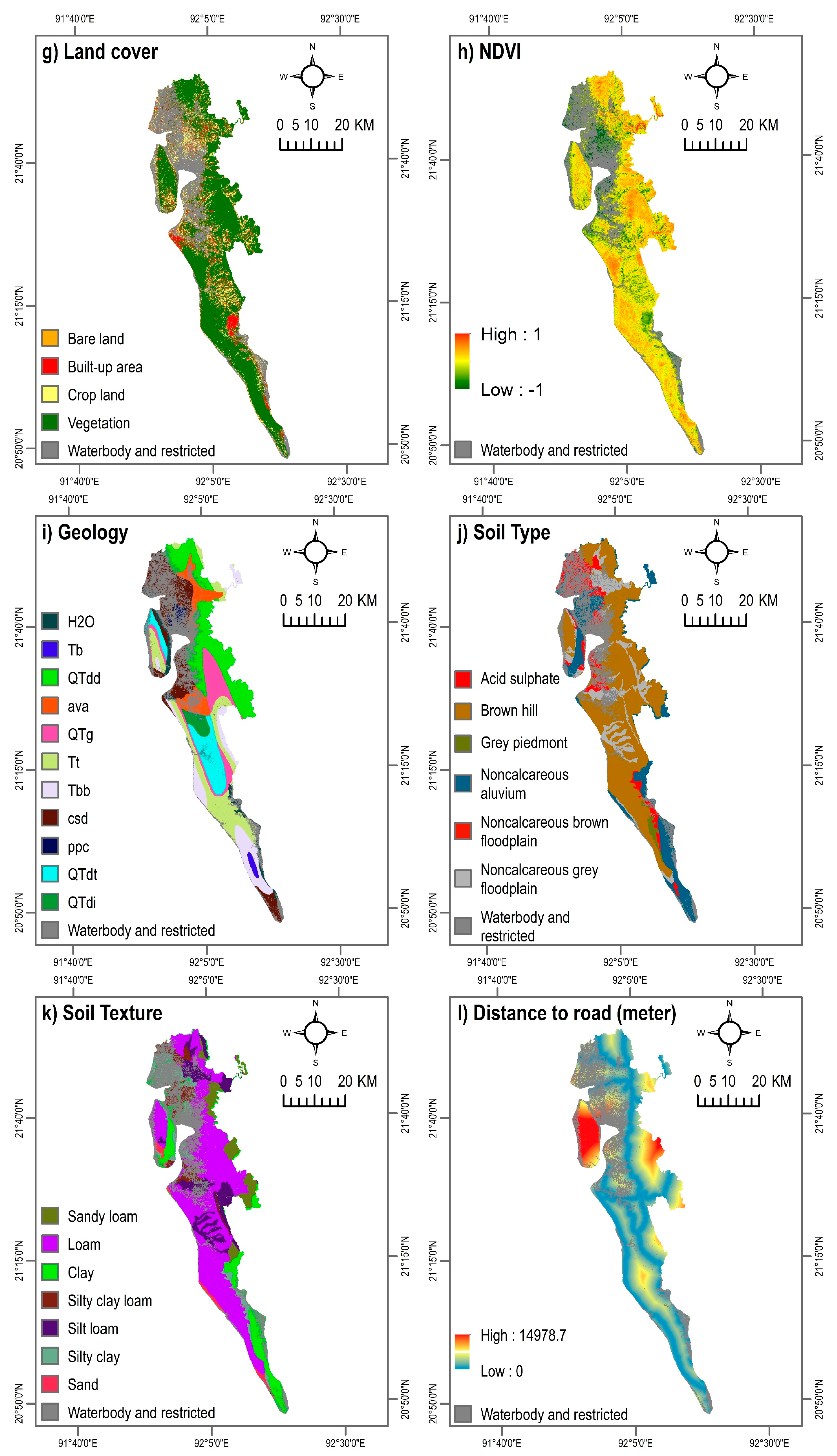
The performance of LSMs depends on the choice of landslide conditioning factors. Numerous studies on LSM have been conducted based on machine learning techniques [1,16,18,23,26,37,38], with various combinations of landslide conditioning factors being used. However, the selection of factors should be (i) based on their degree of affinity with landslide locations, (ii) measurable, (iii) non-redundant, and (iv) based on the knowledge of geomorphological characteristics of the area under study [2]. Based on the knowledge obtained from the literature, as well as, expert knowledge on the study area, a total of 12 variables were selected in this current study (Table 1). Areas with an elevation of less than 5 m, as well as, waterbodies and sandy sea beach areas (waterbody and restricted in Figure 4) were excluded from the LSMs [39].
Topographical and hydrological parameters including aspect, elevation, slope, curvature, and Stream Power Index (SPI) are important factors that limit the density and spatial extent of landslides [2,37,38,40]. Raster maps of aspect, elevation, curvature, slope, and SPI were derived at 30-m spatial resolution from the Advanced Land Observing Satellite (ALOS) Digital Elevation Model (DEM) [28] (Figure 4a–e). Elevation influences landslides primarily by affecting different biophysical parameters and anthropogenic activities. Only a limited number of studies, conducted on a specific basin, found that landslides occur at certain elevations [41]. Elevation can determine the spatial variability of landslides because it is affected by geological tectonics [37]. It can also influence the occurrence of landslides by impacting other causative factors such as slope, curvature, and SPI [42]. Aspect, indicating the direction of slope [43], indirectly influences the distribution of landslide locations by affecting the general physiographic trend of the area and/or the main precipitation direction [37,40]. Slope angle is considered as one of the most influential factors for the occurrence of landslides, as it affects the concentration of moisture and the level of pore pressure, as well as, controls regional hydraulic continuity [2,40]. All of these processes influence slope instability [8]. Curvature is also considered as a landslide influencing factor that directly controls the velocity of water flow, delimiting erosion [8,40]. SPI also determines the erosion potential of the surface [43] and is considered as an essential predictor of landslides [37,38]. Areas with high SPI values indicate a higher erosion potential, while negative values suggest no predicted erosion [44,45]. In this study, a layer of SPI was derived using the following equations in GIS:
where As and β indicates the specific catchment area (m2/m) and slope gradient, respectively [43].
It is widely conceived that various geological factors significantly influence the occurrence of landslides, as these factors often lead to a difference in strength and permeability of rocks and soils [2]. This study considered the three geological factors of surface geology, soil type, and soil texture (Figure 4i–k). Digital geologic and geophysical data of Bangladesh were collected from the U.S. Geological Survey [46]. The surface geology map of the study area includes a total of 11 classes: water (H2O), Bhuban formation (Miocene, Tb), Dupi Tila formations undivided (QTdd), valley alluvium and colluvium (ava), Girujan clay (Pleistocene and Neogene, QTg), Tipam Sandstone (Neogene, Tt), Boka Bil formation (Neogene, Tbb), beach and dune sand (csd), marsh clay and peat (ppc), Dupi Tila formation (Pleistocene and Pliocene, QTdt), and Dihing formation (Pleistocene and Pliocene, QTdi) (Figure 4i). Primary-level parameters such as soil type and soil texture are essential predictors of landslides. These parameters determine the amount of moisture content indicating the degree of stability of the soil [25,37,47,48]. Soil type and soil texture data were collected from the Bangladesh Agricultural Research Council [49].
Other anthropogenic, environmental, and locational factors considered in this study include distance to stream, land cover, normalized difference vegetation index (NDVI), and distance to road (Figure 4f–h,l). The land cover and NDVI maps of the year 2020 were prepared using Landsat satellite images based on the Google Earth Engine Platform. The land cover map was developed applying a supervised classification technique with the Random Forest algorithm. In the case of southern Bangladesh, a recent study demonstrated that this method has a higher classification accuracy compared to other land cover classification techniques [50]. The land cover map contains five classes: bare land, built-up area, crop land, vegetation, and waterbody (Figure 4g). Proximity to roads explains the locations of landslides, as the artificial and natural slopes adjacent to a road are sensitive to this hazard [51]. Road-cuts, excavation, and additional load can induce anthropogenic instability of the soil, promoting landslides [2,5]. A layer of distance to road network was developed using the Euclidian distance algorithm. Likewise, the location of areas with respect to natural drainage channels can also demonstrate the locations of landslides [11], as streams may change the stability of an area by eroding the slopes [5,51]. In this study, distance to stream networks was derived from the ALOS DEM. Again, by applying the Euclidian distance algorithm, a map of distance to stream was generated.
2.4. Multi-Collinearity Analysis of Landslide Conditioning Factors
The selected landslide causative factors could be subject to multi-collinearity; hence, it is necessary to estimate the correlation of independent variables before modelling landslide susceptibility [8]. To eliminate the factors susceptible to multi-collinearity, this study determined variance inflation factors (VIF) [53] of 12 selected landslide conditioning factors using R [54]. VIF is a well-known method to determine the multi-collinearity of landslide conditioning factors [8,55]. A VIF value of a variable exceeding 5 indicates potential serious multicollinearity [53,55]. In this study, the selected landslide conditioning factors yielded VIF values < 2.8, indicating the absence of potential multi-collinearity (Table 1).
2.5. Landslide Susceptibility Modelling
2.5.1. Pre-Processing
Using the binary locations (landslide and non-landslide), values of the selected 12 conditioning factors were extracted in a geographic information system (GIS) environment. As evident in Table 1, eight were continuous variables, while the remaining four variables had discrete characteristics. In order to represent discrete (categorical) variables semantically, they must be considered as a composite feature (where the number of generated binary features and the number of categories are equal). These discrete variables were encoded using a one-hot encoding scheme [31], implying that multiple binary features were generated to represent a single discrete feature. The number of one-hot encoded features depends on the number of variable classes. For instance, there are 11 categories in the geology variable. If a landslide location was found in a geology class, a value 1 was encoded to the class, while the other 10 classes were encoded as 0. This data pre-processing method was applied for all other discrete variables. For each variable, mean and standard deviation were calculated. The mean of each variable was then subtracted from the corresponding value in a variable and divided by the standard deviation. This reduces training time since optimization routines have a smaller parameter space to traverse.
2.5.2. Hyperparameter Optimization
Hyperparameter optimization can improve the accuracy of machine learning algorithm-based models. The process aims to select the optimal hyperparameter values according to the evaluation index [56]. Three approaches are frequently used for optimizing hyperparameters: grid search, random search, and Bayesian optimization [57]. This current study applied the grid search technique along with 5-fold cross-validation on the training set to perform hyperparameter optimization. Hyperparameters that provide the best performance were chosen for final training and testing samples of respective machine learning models. For instance, the optimal number of neighbors of five in the KNN (Table 2) indicates that values of landslide conditioning factors corresponding to a landslide location were compared against the values of landslide predictors of five other sample locations, to obtain the most reliable prediction. Table 2 summarizes the hyperparameters, their search range and optimal values of the four models.
2.5.3. Machine Learning Models
- (1)
- K-Nearest Neighbor (KNN)
The KNN algorithm classifies an instance (landslide or non-landslide) that is mostly represented within its (k) neighbors. The parameter k is often a small positive integer [58]. The proximity between the samples is measured using a distance metric. The distance metric indicates how similar or different are the profiles of conditioning factors for any given two samples. Data points with similar conditioning factors will have a small feature distance between them. Though the model is simple in terms of hyperparameters, it becomes computationally expensive as the number of samples becomes large. The landslide susceptibility associated with a certain set of values of conditioning factors is determined by calculating its distance to each training data point (in high-dimensional feature space). The k nearest data points are used to determine the landslide susceptibility. The dominant susceptibility class within those k nearest neighbors (i.e., the class with the highest number of members in the k members) becomes the class membership of the new data point [14,59].
- (2)
- Multi-Layer Perceptron (MLP)
Multi-Layer Perceptron (MLP) is a type of neural network with one or more hidden layers. Due to the presence of a hidden layer, the internal representations (as higher-order intermediate features) can be learned. Each layer consists of one or more neurons; the outputs (activations a) can be represented by Equation 2 [31]. The output of the ith neuron in the jth layer was obtained by calculating the sum of activations from the previous layer (i − 1) weighted by the parameters of layer i and then passing into an activation function f. Considering that there are several types of activation functions (sigmoid, hyperbolic tangent, rectified linear unit), the choice of activation functions is discussed in Section 2.5.3 (Hyperparameter Optimization). In this study, since a total of 23 features were derived by one-hot encoding during the pre-processing step, the first input layer of the MLP had 23 neurons. The resultant map was represented in terms of the probability of landslide occurrence.
where f is the activation function, is the weight of kth neuron in layer j, is the activation of neuron k in layer j − 1 (the previous layer), j is the layer index, i is the neuron index, and n is the number of neurons in layer j.
- (3)
- Random Forest (RF)
Random forest (RF) is considered as a powerful ensemble-learning method that can be applied for classification, regression, and unsupervised learning [18]. This method has been widely applied in landslide susceptibility mapping [18,56,60]. Ensemble models generally train several weak learners and then take their aggregated outputs to obtain more reliable predictions. The RF algorithm builds weak learners in the form of decision trees. It estimates the mean of outputs of the individual weak learners, as shown in Equation (3). Each weak learner (b) corresponds to a function fb(x). The RF uses bootstrap aggregating where the weak learners train parallelly [31].
where is the ensembled prediction from weak learners, B is the total number of weak learners, b is the weak learner index, and fb(x) is the function for bth weak learner.
- (4)
- Support Vector Machine (SVM)
Support Vector Machine (SVM) is also a widely used machine learning algorithm in landslide susceptibility mapping [8,16,23,26]. This supervised learning method separates the classes with a decision surface that maximizes the margin of class boundaries [8]. The training locations, closest to the optimal hyperplane, are called support vectors [23]. Suppose each sample location has M number of features, the objective of the SVM algorithm is to find a hyperplane in M dimensional feature space that separates the samples of different classes. A hyperplane is R(M−1) dimensional in RM. A hyperplane in R2 is a line, a hyperplane in R3 is a plane, and so on. This hyperplane functions as a decision boundary, which determines the label of a sample (i.e. landslide or non-landslide). The margin around the hyper lane indicates that value exceeding 1 denotes a positive sample (landslide), and a value equal to −1 denotes a negative sample (non-landslide). If X (X1, X2, ………, Xn) is the vector of landslide affecting factor and Yj (Y1, Y2) is the vector of landslide (1) or non-landslide (0) event, the optimal hyperplane can be found by solving Equation (4) [26].
where k is the offset from the origin of the hyperplane, n is the total number of factors that affects landslide, αi is the positive real constant, and k(X, Xi) is the Kernel function. To classify the binary events (landslide or non-landslide), the condition to solve Equation (4) was assumed as below:
where w is the weight vector and φ(xi) is the total number of factors that affects landslide.
2.5.4. Performance Evaluation Methods
The performance of landslide susceptibility models was evaluated using a well-known method called receiver operating characteristic (ROC) curve and subsequent area under the curve (AUC) [1,11,23,31,43]. The ROC curves were developed using the 40% sample testing data. The ROC curve indicates the performance of a binary classifier system, representing sensitivity as a function of the false positive rate (1-specificity).
The sensitivity of a model is the ratio of the number of true positives to the sum of the number of true positives and false negatives. The specificity is the ratio of the number of true negatives to the sum of the number of true negatives and false positives. The ROC curve can be developed by plotting sensitivity in the y-axis against the cumulative distribution function of the false positive rate in the x-axis. The estimated AUC value can be categorized as poor (0.5–0.6), average (0.6–0.7), good (0.7–0.8), very good (0.8–0.9), and excellent (0.9–1) [1,43,60]. Besides, various statistical indices such as overall accuracy, precision, recall, and F1-score were estimated by developing a confusion matrix [1,11,43].
2.6. Evaluation of Spatial Agreement and Optimizing Prediction Map
To evaluate the inter-model agreeability, a pixel-wise agreement between two machine learning algorithms was estimated. Therefore, Pearson’s correlation coefficient was estimated for a total of six possible combinations of machine learning model-based landslide susceptibility maps. Here, Pearson’s correlation coefficient indicates the covariance of landslide predictions, obtained by using two algorithms, divided by the product of their standard deviations. The correlation coefficient can range from +1 to −1, where values zero as indicating no agreement and ±0.29 as low degree, ±0.30–±0.49 as moderate degree, ±0.50 to <±1 as high degree, and ±1 as perfect agreement [60].
Following the evaluation of spatial agreement, an optimized landslide prediction map was developed combining susceptibility maps generated by applying the four machine learning algorithms. The combined map was developed by following a methodology proposed by Rossi, Guzzetti, Reichenbach, Mondini, and Peruccacci [22], where they established a logistic regression (LR) model. The LR model included binary landslide and non-landslide locations as the dependent variable and the results of the four landslide susceptibility models as the independent variables. The obtained regression coefficients were incorporated in Equation (6) [43] in GIS to derive the probability (P) of landslides in the study area.
where z is the linear combination of independent variables which was estimated using the following equation:
where θ0 is the intercept of the model, θi (i = 1, 2, …, n) indicates the regression coefficient of independent variables, and xi (i = 1, 2, …, n) represents the n number of independent variables. Validation of the resultant combined model was performed by developing the ROC curve by using the 40% testing data.
3. Results
3.1. Landslide Susceptibility Modelling
3.1.1. Landslide Prediction
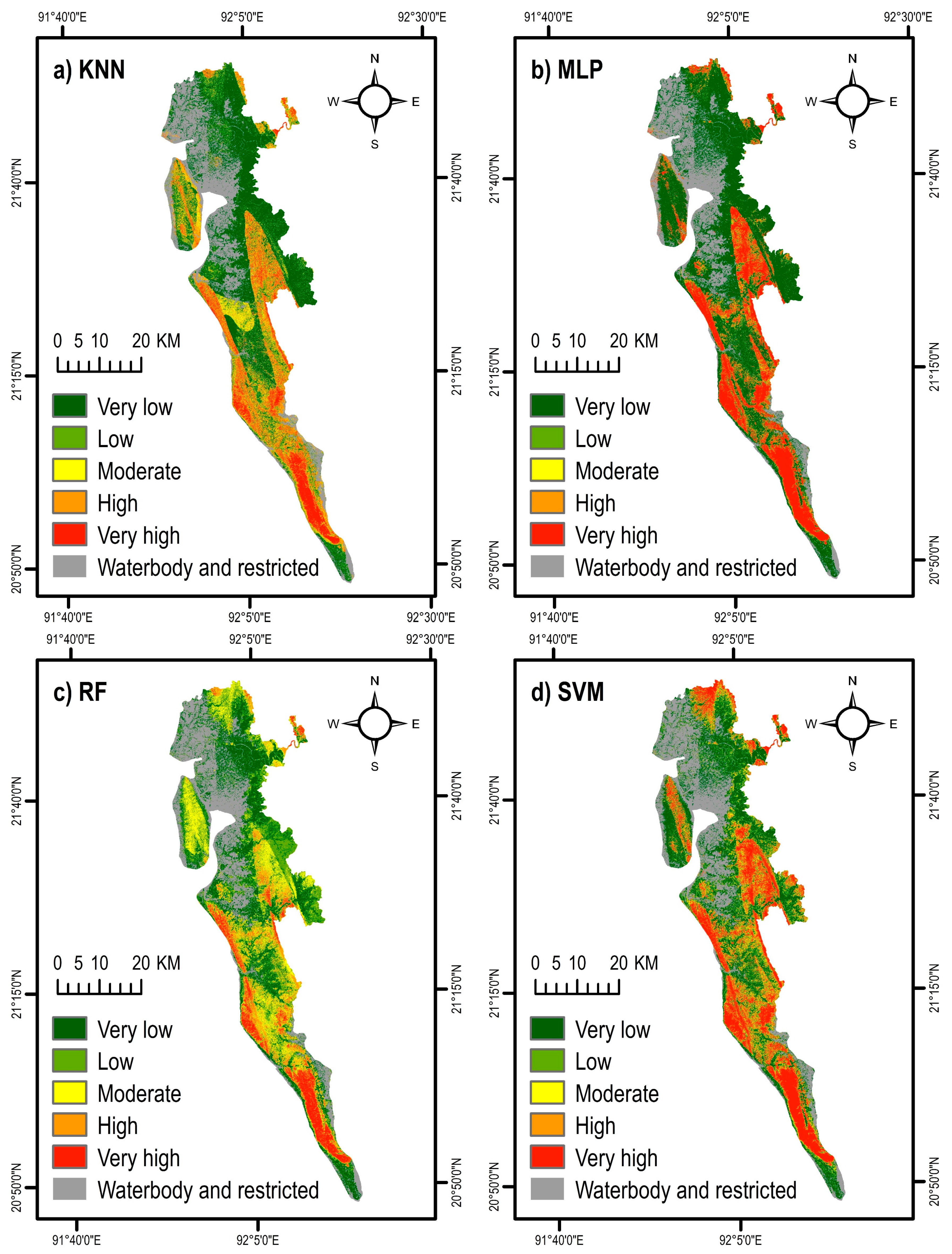
Figure 5 shows landslide susceptibility maps of Cox’s Bazar district developed by applying the four machine learning algorithms. The generated landslide probability maps were classified into five categories each by applying the Jenks natural breaks classification method in GIS: (i) very low (0–0.1), (ii) low (0.11–0.3), (iii) medium (0.31–0.5), (iv) high (0.51–0.85), and (v) very high (0.86–1). As evident in Figure 6, the proportion of landslide susceptible area varied from one model to another. Among all methods, the SVM resulted in the highest proportion of area (38.7%) susceptible to the landslide of ‘high’ and ‘very high’ severity, while the Random Forest (RF) algorithm yielded a relatively lower proportion (23.1%) of landslide susceptible area. Likewise, the ratio of the population exposed to ‘high’ and ‘very high’ landslide susceptible zones varied for different algorithms. For all the four methods, the percentage of landslide exposed population ranged between 34% to 48% (Figure 6).
3.1.2. Evaluation of Models’ Performance
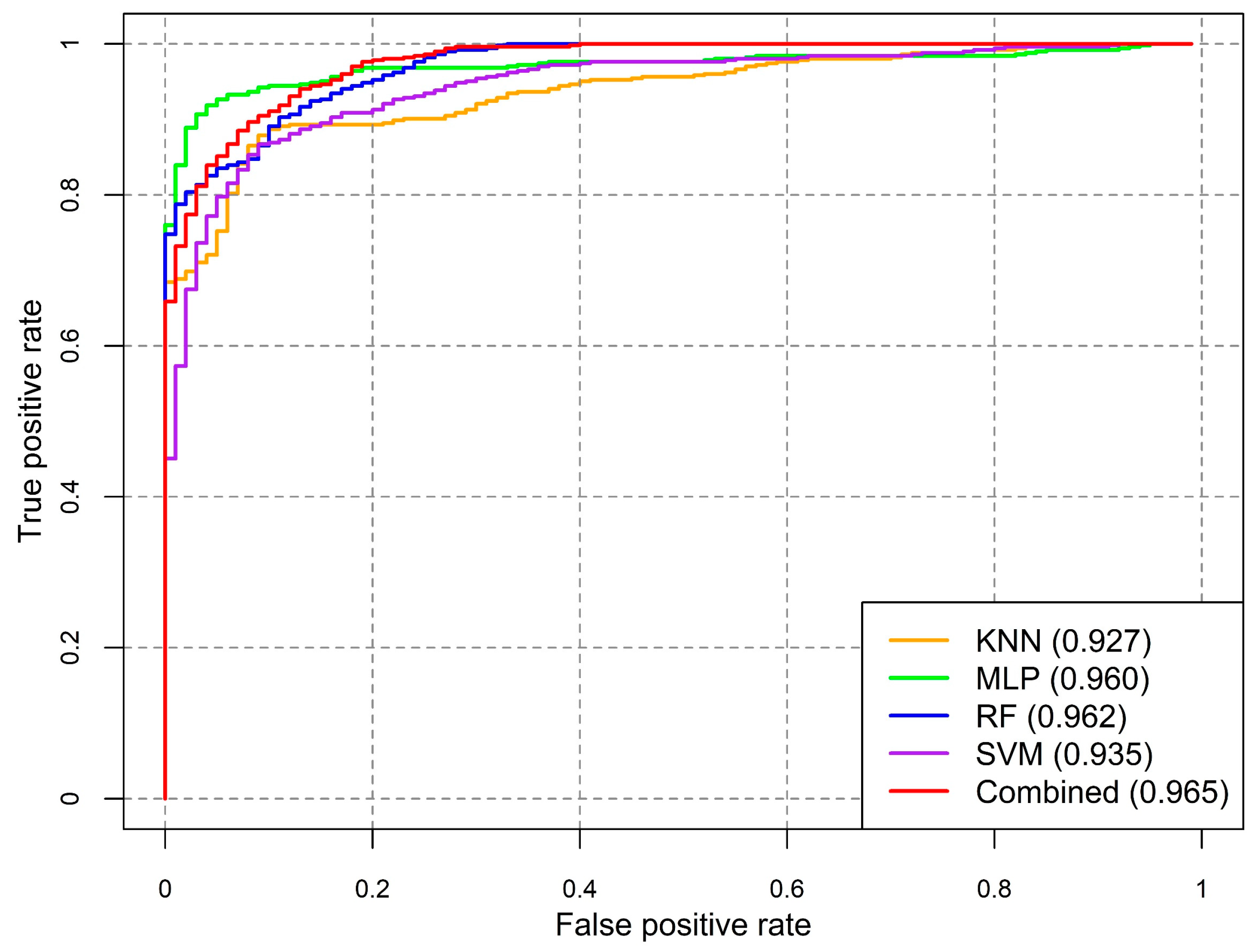
To evaluate the performance of various landslide susceptibility models, a performance matrix was derived using the test samples (40% of the total data) (Table 3). The performance evaluation indices indicated a very high prediction accuracy of all the models. In terms of overall accuracy, the RF classifier resulted in the highest accuracy (96.63%), followed by the MLP (95.45%), SVM (94.06%), and KNN (90.69%). However, the overall accuracy is a universal metric, hence, it does not indicate which specific classes were being inaccurately classified. To obtain further insights into the agreement between the observed and modelled locations (landslide and non-landslide)—precision, F1-score, and recall were estimated (Table 3). The RF classifier achieved the best accuracy with respect to all performance indicators. The MLP followed closely and consistently in terms of all indicators. In relation to the estimated AUC values, the RF classifier yielded the highest accuracy (0.962), followed by the MLP (0.960), SVM (0.935), and KNN (0.927) (Figure 7). The relatively greater values of performance indicators of RF and MLP can be attributed to their ability to learn complex relationships between geospatial characteristics of an area and the occurrence of landslides [17,18,60].
3.2. Spatial Agreement of Various Methods
This study developed a correlation matrix by comparing pixel-wise landslide probabilities between various methods (Figure 8) to evaluate the extent of agreement of one landslide susceptibility model over another. Although the values of AUC were very similar for various methods (Figure 7), a substantial difference in the agreement was observed in LSMs obtained using the different techniques. Overall, the correlation coefficient ranges from 0.69 to 0.85 (Figure 8). The combinations of SVM-RF resulted in the highest degree of the agreement, while the KNN-SVM yielded the lowest agreement.
3.3. Aggregated Landslide Susceptibility Mapping
Since spatial heterogeneity in landslide prediction exists between the different machine learning-based approaches, an aggregated susceptibility map combining the outputs of all algorithms would minimize the uncertainty of individual methods. In this study, a regression-based approach was adopted. A multivariate logistic regression (LR) was established incorporating the binary landslide inventory data as the dependent variable and the results of the four landslide susceptibility models as independent variables. The outcome of the LR model is summarized in Table 4. Among the four models, the MLP, RF, and SVM were statistically significant (p-value < 0.05). The coefficient of determinants (R2) of 0.80 indicates a very good model performance. In relation to the estimated regression coefficients, the RF model had the highest degree of agreement with the landslide inventory, followed by the MLP, SVM, and KNN. The pattern of influence of various models in predicting landslides corresponds to their level of accuracy in terms of their respective AUC values (Figure 7).
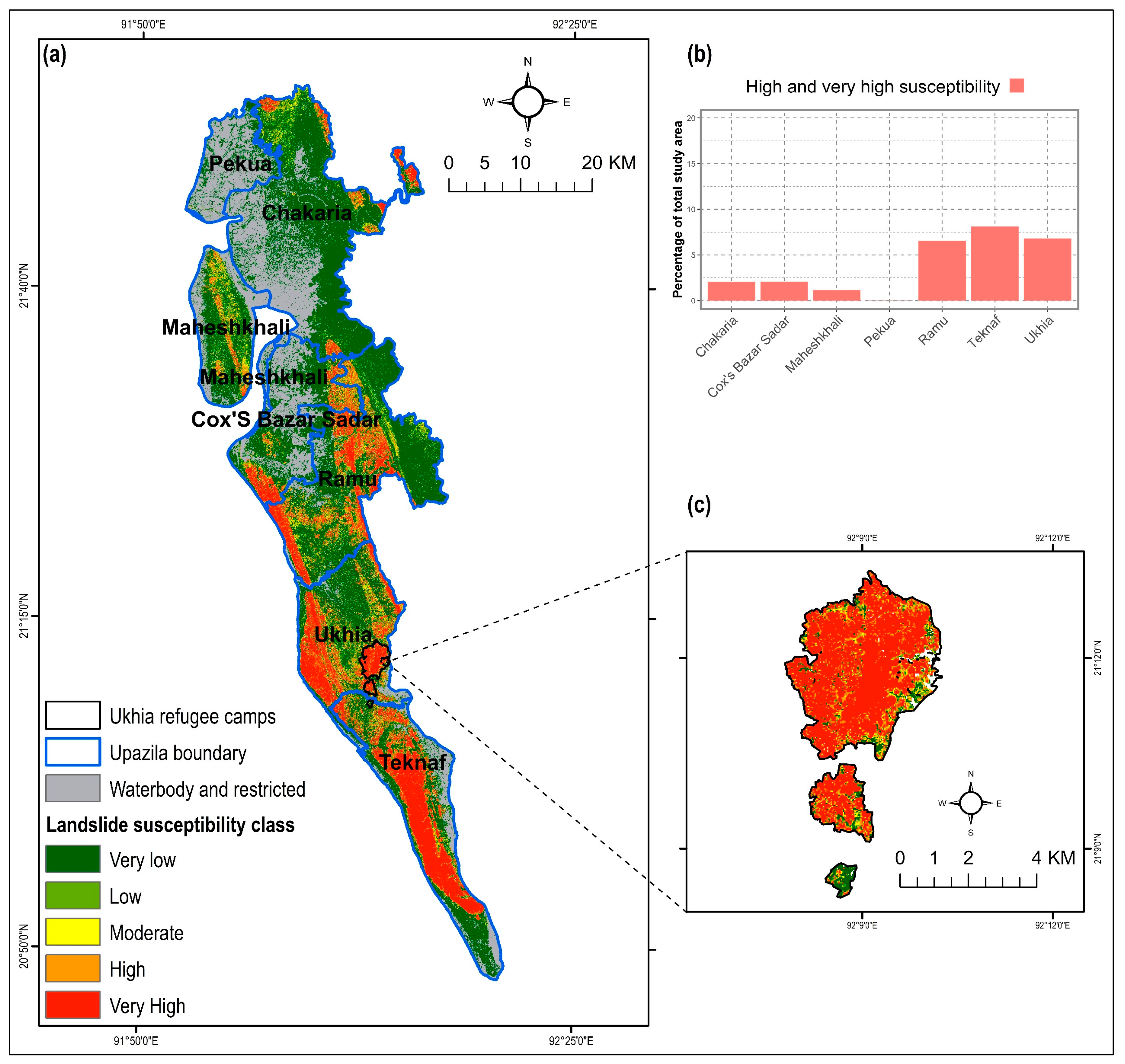
The estimated LR coefficients of the four models and intercept were incorporated in Equation (6) to derive the combined LSM. Again, the resultant aggregated map was categorized into five classes applying the Jenks Natural Break algorithm (Figure 9). The combined susceptibility map yielded the highest AUC value (0.965) compared to the single susceptibility forecasts (Figure 7). About 26.8% of the total study area was within the ‘high’ and ‘very high’ landslide susceptible zones, where approximately 21.7% of total population inhabit (Figure 6). In respect to spatial agreement, the combined LSM resulted in greater spatial agreement with the all four models, with the correlation coefficient ranging between 0.85 and 0.92 (Figure 8).
The extent of landslide susceptible areas varies in different sub-districts (Upazila) of Cox’s Bazar. Teknaf Upazila is the most susceptible, where more than 8% of the total study area was susceptible to landslides of ‘high and ‘very high’ severity (Figure 9b). A substantial proportion of area (7% of the study area) in Ukhia sub-district was also susceptible. The Rohingya refugee camps in this area were located within high and very high landslide susceptible zones. Various recent studies also found that changes in the geomorphological, hydrological, and anthropogenic environments due to the Rohingya influx caused their settlement areas vulnerable to landslides [11,31].
4. Discussion
The spatial disagreement in prediction among various techniques creates challenges in selecting the most suitable susceptibility map for managing landslide hazards [9,21,22]. The current study seeks to address this challenge by estimating the extent of spatial agreement, as well as, proposing a method to combine landslide susceptibility maps and thus incorporating the valid results of various models. The study focused on the Cox’s Bazar district of Bangladesh, which is well known as being vulnerable to landslide disasters [11,12,31]. First, LSMs were developed by applying four machine learning algorithms—K-Nearest Neighbor (KNN), Multi-Layer Perceptron (MLP), Random Forest (RF), and Support Vector Machine (SVM)—featuring hyperparameter optimization. In comparison to the existing studies on LSM of Cox’s Bazar district [11,12,31], this current study employed up-to-date data of landslide conditioning factors. In addition, it restricted low-lying areas (waterbodies and elevation < 5m) in susceptibility mapping, otherwise, the resultant maps would have been prone to overestimation of landslide susceptible zones, as was the case of some recent studies. While evaluating the models’ performance, all of them yielded very high prediction accuracy, with the AUC values ranging between 0.927 to 0.962. The results of various recent studies have also ascertained that different machine learning-based models yielded high accuracy in predicting landslides [1,15,17,26,27,61].
This study hypothesized that different susceptibility models can result in different LSMs, despite incorporating similar landslide inventory data. The assessment of spatial agreement between various models revealed spatial heterogeneity in landslide predictions, with the estimated pixel-wise correlation coefficients of landslide probability between various models ranging from 0.69 to 0.85. The spatial distribution of landslide susceptibility obtained in this study was also different than that of a recent study conducted in Cox’s Bazar district of Bangladesh [11]. This highlights the uncertainty in landslide predictions of various models, despite their considerable prediction accuracy in terms of the AUC values. Most of the existing studies on machine learning-based LSM had a major focus on identifying the most suitable method for predicting this natural phenomenon [1,8,18,23,60], while little attention has been given in analyzing uncertainties resulting from the spatial disagreement in landslide prediction [9]. The current study is the first case study-based contribution to investigate this major gap in the existing literature.
This study further developed a combined LSM by integrating the results of the four machine learning-based landslide predictions, adopting a method proposed by Rossi, Guzzetti, Reichenbach, Mondini, and Peruccacci [22]. The result indicates an improvement in landslide prediction accuracy. Existing studies, which applied multiple machine learning algorithms to map landslide susceptibility, mainly evaluated different methods based on quantitative measures [8,16,18]. Whilst quantitative measures of model fit are useful, they are not conclusive in determining the efficacy and reliability of susceptibility assessment [22]. A combined landslide susceptibility map that this study developed would help to minimize the uncertainties of individual methods.
5. Conclusions
Predicting a complex natural phenomenon such as a landslide is a challenging task and subject to considerable uncertainties. An accurate prediction of landslides is the prerequisite for managing this hazard. In this study, the spatial association in landslide prediction between various machine learning-based models was analyzed to quantify the spatial agreement of predicted landslide susceptibility. By addressing uncertainties in various models, this study also developed a landslide susceptibility map combining the outcomes from various models. The results indicate an improvement in landslide prediction compared to the individual models.
Despite achieving an improved result in landslide prediction, this study has some limitations that could be addressed in future results. Landslide inventory data used in this study was developed based on various secondary sources and validated through fieldwork [11]. Scarcity of data, including detailed landslide inventory on the study area, made it difficult to model a landslide more accurately. Accuracy of the LSM results depended on input parameters used, particularly the DEM. The ALOS DEM of 30-m resolution used in this study had a low root-mean-square error (1.78 m) in vertical accuracy and was considered to be the most accurate freely available DEM [43,62]. However, for future research, high-resolution DEM could be employed to improve the existing landslide susceptibility modelling frameworks.
This study is an attempt to integrate results of multiple machine learning-based landslide susceptibility models to minimize uncertainties and improve landslide predictions. The modelling framework used in this study could be transferred to other landslide-susceptible regions. Landslide susceptibility maps can enable urban planners in identifying suitable areas for urban development [63]. The combined landslide susceptibility map of Cox’s Bazar district could be useful to policymakers and practitioners in sequencing and prioritizing interventions in managing landslides. The proposed model is an advancement in the existing landslide susceptibility models that intends to predict landslides more accurately. The results of this model could be utilized in improving the existing landslide early warning system [11], to strengthen landslide disaster risk mitigation strategies to support for the resilient future of inhabitants of the study area.
Author Contributions
Conceptualization, M.S.G.A. and B.A.; methodology, M.S.G.A., M.S.R., and N.A.; software, M.S.G.A., M.S.R., N.A., and R.M.R.; validation, M.S.G.A., M.S.R., and N.A.; formal analysis, M.S.G.A., M.S.R., and N.A.; investigation, M.S.G.A., B.A., R.M.R., and M.F.R.; resources, M.S.G.A., M.F.R., and B.A.; data curation, M.S.G.A. and B.A.; writing—original draft preparation, M.S.G.A.; writing—review and editing, M.S.G.A. and B.A.; visualization, M.S.G.A. and B.A.; supervision, B.A. All authors have read and agreed to the published version of the manuscript.
Funding
This research received no external funding.
Conflicts of Interest
The authors declare no conflict of interest.
References
- Chen, W.; Peng, J.; Hong, H.; Shahabi, H.; Pradhan, B.; Liu, J.; Zhu, A.-X.; Pei, X.; Duan, Z. Landslide susceptibility modelling using GIS-based machine learning techniques for Chongren County, Jiangxi Province, China. Sci. Total Environ. 2018, 626, 1121–1135. [Google Scholar] [CrossRef] [PubMed]
- Ayalew, L.; Yamagishi, H. The application of GIS-based logistic regression for landslide susceptibility mapping in the Kakuda-Yahiko Mountains, Central Japan. Geomorphology 2005, 65, 15–31. [Google Scholar] [CrossRef]
- Shahabi, H.; Hashim, M. Landslide susceptibility mapping using GIS-based statistical models and Remote sensing data in tropical environment. Sci. Rep. 2015, 5, 1–15. [Google Scholar] [CrossRef] [PubMed] [Green Version]
- Qiao, G.; Lu, P.; Scaioni, M.; Xu, S.; Tong, X.; Feng, T.; Wu, H.; Chen, W.; Tian, Y.; Wang, W. Landslide investigation with remote sensing and sensor network: From susceptibility mapping and scaled-down simulation towards in situ sensor network design. Remote Sens. 2013, 5, 4319–4346. [Google Scholar] [CrossRef] [Green Version]
- Pourghasemi, H.R.; Pradhan, B.; Gokceoglu, C. Application of fuzzy logic and analytical hierarchy process (AHP) to landslide susceptibility mapping at Haraz watershed, Iran. Nat. Hazards 2012, 63, 965–996. [Google Scholar] [CrossRef]
- Scaioni, M. Remote sensing for landslide investigations: From research into practice. Remote Sens. 2013, 5, 5488–5492. [Google Scholar] [CrossRef] [Green Version]
- Kalantar, B.; Ueda, N.; Saeidi, V.; Ahmadi, K.; Halin, A.A.; Shabani, F. Landslide Susceptibility Mapping: Machine and Ensemble Learning Based on Remote Sensing Big Data. Remote Sens. 2020, 12, 1737. [Google Scholar] [CrossRef]
- Chen, W.; Pourghasemi, H.R.; Panahi, M.; Kornejady, A.; Wang, J.; Xie, X.; Cao, S. Spatial prediction of landslide susceptibility using an adaptive neuro-fuzzy inference system combined with frequency ratio, generalized additive model, and support vector machine techniques. Geomorphology 2017, 297, 69–85. [Google Scholar] [CrossRef]
- Sterlacchini, S.; Ballabio, C.; Blahut, J.; Masetti, M.; Sorichetta, A. Spatial agreement of predicted patterns in landslide susceptibility maps. Geomorphology 2011, 125, 51–61. [Google Scholar] [CrossRef]
- Ahmed, B.; Dewan, A. Application of bivariate and multivariate statistical techniques in landslide susceptibility modeling in Chittagong City Corporation, Bangladesh. Remote Sens. 2017, 9, 304. [Google Scholar] [CrossRef] [Green Version]
- Ahmed, B.; Rahman, M.S.; Sammonds, P.; Islam, R.; Uddin, K. Application of geospatial technologies in developing a dynamic landslide early warning system in a humanitarian context: The Rohingya refugee crisis in Cox’s Bazar, Bangladesh. Geomat. Nat. Hazards Risk 2020, 11, 446–468. [Google Scholar] [CrossRef]
- Ahmed, B. Landslide susceptibility modelling applying user-defined weighting and data-driven statistical techniques in Cox’s Bazar Municipality, Bangladesh. Nat. Hazards 2015, 79, 1707–1737. [Google Scholar] [CrossRef]
- Althuwaynee, O.F.; Pradhan, B.; Park, H.J.; Lee, J.H. A novel ensemble bivariate statistical evidential belief function with knowledge-based analytical hierarchy process and multivariate statistical logistic regression for landslide susceptibility mapping. Catena 2014, 114, 21–36. [Google Scholar] [CrossRef]
- Souza, F.; Ebecken, N. A data mining approach to landslide prediction. WIT Trans. Inf. Commun. Technol. 2004, 33, 423–432. [Google Scholar]
- Marjanovic, M.; Bajat, B.; Kovacevic, M. Landslide susceptibility assessment with machine learning algorithms. In Proceedings of the 2009 International Conference on Intelligent Networking and Collaborative Systems, Barcelona, Spain, 4–6 November 2009; pp. 273–278. [Google Scholar]
- Yao, X.; Tham, L.; Dai, F. Landslide susceptibility mapping based on support vector machine: A case study on natural slopes of Hong Kong, China. Geomorphology 2008, 101, 572–582. [Google Scholar] [CrossRef]
- Zare, M.; Pourghasemi, H.R.; Vafakhah, M.; Pradhan, B. Landslide susceptibility mapping at Vaz Watershed (Iran) using an artificial neural network model: A comparison between multilayer perceptron (MLP) and radial basic function (RBF) algorithms. Arab. J. Geosci. 2013, 6, 2873–2888. [Google Scholar] [CrossRef]
- Chen, W.; Xie, X.; Wang, J.; Pradhan, B.; Hong, H.; Bui, D.T.; Duan, Z.; Ma, J. A comparative study of logistic model tree, random forest, and classification and regression tree models for spatial prediction of landslide susceptibility. Catena 2017, 151, 147–160. [Google Scholar] [CrossRef] [Green Version]
- Feizizadeh, B.; Blaschke, T. An uncertainty and sensitivity analysis approach for GIS-based multicriteria landslide susceptibility mapping. Int. J. Geogr. Inf. Sci. 2014, 28, 610–638. [Google Scholar] [CrossRef] [Green Version]
- Crosetto, M.; Tarantola, S.; Saltelli, A. Sensitivity and uncertainty analysis in spatial modelling based on GIS. Agric. Ecosyst. Environ. 2000, 81, 71–79. [Google Scholar] [CrossRef]
- Guzzetti, F.; Reichenbach, P.; Ardizzone, F.; Cardinali, M.; Galli, M. Estimating the quality of landslide susceptibility models. Geomorphology 2006, 81, 166–184. [Google Scholar] [CrossRef]
- Rossi, M.; Guzzetti, F.; Reichenbach, P.; Mondini, A.C.; Peruccacci, S. Optimal landslide susceptibility zonation based on multiple forecasts. Geomorphology 2010, 114, 129–142. [Google Scholar] [CrossRef]
- Pradhan, B. A comparative study on the predictive ability of the decision tree, support vector machine and neuro-fuzzy models in landslide susceptibility mapping using GIS. Comput. Geosci. 2013, 51, 350–365. [Google Scholar] [CrossRef]
- Valencia Ortiz, J.A.; Martínez-Graña, A.M. A neural network model applied to landslide susceptibility analysis (Capitanejo, Colombia). Geomat. Nat. Hazards Risk 2018, 9, 1106–1128. [Google Scholar] [CrossRef] [Green Version]
- Lee, S.; Ryu, J.H.; Min, K.; Won, J.S. Landslide susceptibility analysis using GIS and artificial neural network. Earth Surf. Proc. Landf. J. Br. Geomorphol. Res. Group 2003, 28, 1361–1376. [Google Scholar] [CrossRef]
- Marjanović, M.; Kovačević, M.; Bajat, B.; Voženílek, V. Landslide susceptibility assessment using SVM machine learning algorithm. Eng. Geol. 2011, 123, 225–234. [Google Scholar] [CrossRef]
- Shirzadi, A.; Soliamani, K.; Habibnejhad, M.; Kavian, A.; Chapi, K.; Shahabi, H.; Chen, W.; Khosravi, K.; Thai Pham, B.; Pradhan, B. Novel GIS based machine learning algorithms for shallow landslide susceptibility mapping. Sensors 2018, 18, 3777. [Google Scholar] [CrossRef] [PubMed]
- JAXA. ALOS Global Digital Surface Model “ALOS World 3D-30m (AW3D30)”; Japan Aerospace Exploration Agency (JAXA): Tokyo, Japan, 2015. [Google Scholar]
- WorldPop. The spatial distribution of population in 2020, Bangladesh. In Global High Resolution Population Denominators Project-Funded by The Bill and Melinda Gates Foundation (OPP1134076); University of Southampton: Southampton, UK, 2020. [Google Scholar] [CrossRef]
- UNHCR. Rohingya Refugees Population by Location at Camp and Union Level-Cox’s Bazar, 21 September 2020 ed.; United Nations High Commissioner for Refugees: Geneva, Switzerland, 2020. [Google Scholar]
- Ahmed, N.; Firoze, A.; Rahman, R.M. Machine learning for predicting landslide risk of Rohingya refugee camp infrastructure. J. Inf. Telecommun. 2020, 4, 175–198. [Google Scholar] [CrossRef] [Green Version]
- Paul, R.; Hussain, Z. Landslide, Floods Kill 156 in Bangladesh, India; Toll Could Rise. 2017. Available online: https://www.reuters.com/article/us-bangladesh-landslides-idUSKBN1950AI (accessed on 6 September 2020).
- UNHCR. Location of Rohingya Refugees in Cox’s Bazar as of 31 July 2020 sourced from RRRC-UNHCR Family Counting Exercise Data; United Nations High Commissioner for Refugees (UNHCR): Geneva, Switzerland, 2020. [Google Scholar]
- Huang, F.; Yin, K.; Huang, J.; Gui, L.; Wang, P. Landslide susceptibility mapping based on self-organizing-map network and extreme learning machine. Eng. Geol. 2017, 223, 11–22. [Google Scholar] [CrossRef]
- Tsangaratos, P.; Benardos, A. Estimating landslide susceptibility through a artificial neural network classifier. Nat. Hazards 2014, 74, 1489–1516. [Google Scholar] [CrossRef]
- Gorsevski, P.V.; Gessler, P.E.; Foltz, R.B.; Elliot, W.J. Spatial prediction of landslide hazard using logistic regression and ROC analysis. Trans. GIS 2006, 10, 395–415. [Google Scholar] [CrossRef]
- Chen, W.; Li, Y. GIS-based evaluation of landslide susceptibility using hybrid computational intelligence models. Catena 2020, 195, 104777. [Google Scholar] [CrossRef]
- Moayedi, H.; Mehrabi, M.; Mosallanezhad, M.; Rashid, A.S.A.; Pradhan, B. Modification of landslide susceptibility mapping using optimized PSO-ANN technique. Eng. Comput. 2019, 35, 967–984. [Google Scholar] [CrossRef]
- Fu, S.; Chen, L.; Woldai, T.; Yin, K.; Gui, L.; Li, D.; Du, J.; Zhou, C.; Xu, Y.; Lian, Z. Landslide hazard probability and risk assessment at the community level: A case of western Hubei, China. Nat. Hazards Earth Syst. Sci. 2020, 20, 581–601. [Google Scholar] [CrossRef] [Green Version]
- Duman, T.; Can, T.; Gokceoglu, C.; Nefeslioglu, H.; Sonmez, H. Application of logistic regression for landslide susceptibility zoning of Cekmece Area, Istanbul, Turkey. Environ. Geol. 2006, 51, 241–256. [Google Scholar] [CrossRef]
- Gomez, H.; Kavzoglu, T. Assessment of shallow landslide susceptibility using artificial neural networks in Jabonosa River Basin, Venezuela. Eng. Geol. 2005, 78, 11–27. [Google Scholar] [CrossRef]
- Chen, W.; Shahabi, H.; Shirzadi, A.; Li, T.; Guo, C.; Hong, H.; Li, W.; Pan, D.; Hui, J.; Ma, M. A novel ensemble approach of bivariate statistical-based logistic model tree classifier for landslide susceptibility assessment. Geocarto Int. 2018, 33, 1398–1420. [Google Scholar] [CrossRef]
- Adnan, M.S.G.; Talchabhadel, R.; Nakagawa, H.; Hall, J.W. The potential of Tidal River Management for flood alleviation in South Western Bangladesh. Sci. Total Environ. 2020, 731, 138747. [Google Scholar] [CrossRef]
- Bannari, A.; Ghadeer, A.; El-Battay, A.; Hameed, N.A.; Rouai, M. Detection of Areas Associated with Flash Floods and Erosion Caused by Rainfall Storm Using Topographic Attributes, Hydrologic Indices, and GIS; Springer: Cham, Switzerland, 2017; pp. 155–174. [Google Scholar]
- Thalacker, R. Mapping Techniques For Soil Erosion: Modeling Stream Power Index in Eastern North Dakota; University of North Dakota: Grand Forks, ND, USA, 2014. [Google Scholar]
- Persits, F.M.; Wandrey, C.J.; Milici, R.C.; Manwar, A. Digital Geologic and Geophysical Data of Bangladesh; 97-470H; US Geological Survey: Reston, VA, USA, 2001. [Google Scholar]
- Dahal, R.K.; Hasegawa, S.; Nonomura, A.; Yamanaka, M.; Masuda, T.; Nishino, K. GIS-based weights-of-evidence modelling of rainfall-induced landslides in small catchments for landslide susceptibility mapping. Environ. Geol. 2008, 54, 311–324. [Google Scholar] [CrossRef]
- Hong, Y.; Adler, R.; Huffman, G. Use of satellite remote sensing data in the mapping of global landslide susceptibility. Nat. Hazards 2007, 43, 245–256. [Google Scholar] [CrossRef] [Green Version]
- BARC. Land Resource Information Management System; Bangladesh Agricultural Research Council (BARC): Dhaka, Bangladesh, 2014. [Google Scholar]
- Abdullah, A.Y.M.; Masrur, A.; Adnan, M.S.G.; Baky, M.A.A.; Hassan, Q.K.; Dewan, A. Spatio-Temporal Patterns of Land Use/Land Cover Change in the Heterogeneous Coastal Region of Bangladesh between 1990 and 2017. Remote Sens. 2019, 11, 790. [Google Scholar] [CrossRef] [Green Version]
- Rozos, D.; Bathrellos, G.; Skillodimou, H. Comparison of the implementation of rock engineering system and analytic hierarchy process methods, upon landslide susceptibility mapping, using GIS: A case study from the Eastern Achaia County of Peloponnesus, Greece. Environ. Earth Sci. 2011, 63, 49–63. [Google Scholar] [CrossRef]
- WARPO. National Water Resources Database (NWRD); Water Resources Planning Organization (WARPO): Dhaka, Bangladesh, 2018. Available online: http://warpo.gov.bd/index.php/home/bnwrd (accessed on 18 August 2020).
- Midi, H.; Sarkar, S.K.; Rana, S. Collinearity diagnostics of binary logistic regression model. J. Interdiscip. Math. 2010, 13, 253–267. [Google Scholar] [CrossRef]
- Fox, J.; Weisberg, S.; Price, B.; Adler, D.; Bates, D.; Baud-Bovy, G.; Bolker, B.; Ellison, S.; Firth, D.; Friendly, M. Package ‘Car’; R Foundation for Statistical Computing: Vienna, Austria, 2018. [Google Scholar]
- Bai, S.; Lü, G.; Wang, J.; Zhou, P.; Ding, L. GIS-based rare events logistic regression for landslide-susceptibility mapping of Lianyungang, China. Environ. Earth Sci. 2011, 62, 139–149. [Google Scholar] [CrossRef]
- Sun, D.; Wen, H.; Wang, D.; Xu, J. A random forest model of landslide susceptibility mapping based on hyperparameter optimization using Bayes algorithm. Geomorphology 2020, 362, 107201. [Google Scholar] [CrossRef]
- Sameen, M.I.; Pradhan, B.; Lee, S. Application of convolutional neural networks featuring Bayesian optimization for landslide susceptibility assessment. Catena 2020, 186, 104249. [Google Scholar] [CrossRef]
- Sameen, M.I.; Pradhan, B.; Bui, D.T.; Alamri, A.M. Systematic sample subdividing strategy for training landslide susceptibility models. Catena 2020, 187, 104358. [Google Scholar] [CrossRef]
- Cheng, G.; Guo, L.; Zhao, T.; Han, J.; Li, H.; Fang, J. Automatic landslide detection from remote-sensing imagery using a scene classification method based on BoVW and pLSA. Int. J. Remote Sens. 2013, 34, 45–59. [Google Scholar] [CrossRef]
- Chen, W.; Zhang, S.; Li, R.; Shahabi, H. Performance evaluation of the GIS-based data mining techniques of best-first decision tree, random forest, and naïve Bayes tree for landslide susceptibility modeling. Sci. Total Environ. 2018, 644, 1006–1018. [Google Scholar] [CrossRef]
- Kadavi, P.R.; Lee, C.-W.; Lee, S. Application of ensemble-based machine learning models to landslide susceptibility mapping. Remote Sens. 2018, 10, 1252. [Google Scholar] [CrossRef] [Green Version]
- Rabby, Y.W.; Ishtiaque, A.; Rahman, M. Evaluating the Effects of Digital Elevation Models in Landslide Susceptibility Mapping in Rangamati District, Bangladesh. Remote Sens. 2020, 12, 2718. [Google Scholar] [CrossRef]
- Bathrellos, G.D.; Skilodimou, H.D.; Chousianitis, K.; Youssef, A.M.; Pradhan, B. Suitability estimation for urban development using multi-hazard assessment map. Sci. Total Environ. 2017, 575, 119–134. [Google Scholar] [CrossRef] [PubMed]
Publisher’s Note: MDPI stays neutral with regard to jurisdictional claims in published maps and institutional affiliations. |
Figure 1.
(a) Location map of Cox’s Bazar district in Bangladesh; and (b) the sub-districts of Cox’s Bazar district. Digital Elevation Model (DEM) source: [28]
Figure 1.
(a) Location map of Cox’s Bazar district in Bangladesh; and (b) the sub-districts of Cox’s Bazar district. Digital Elevation Model (DEM) source: [28]
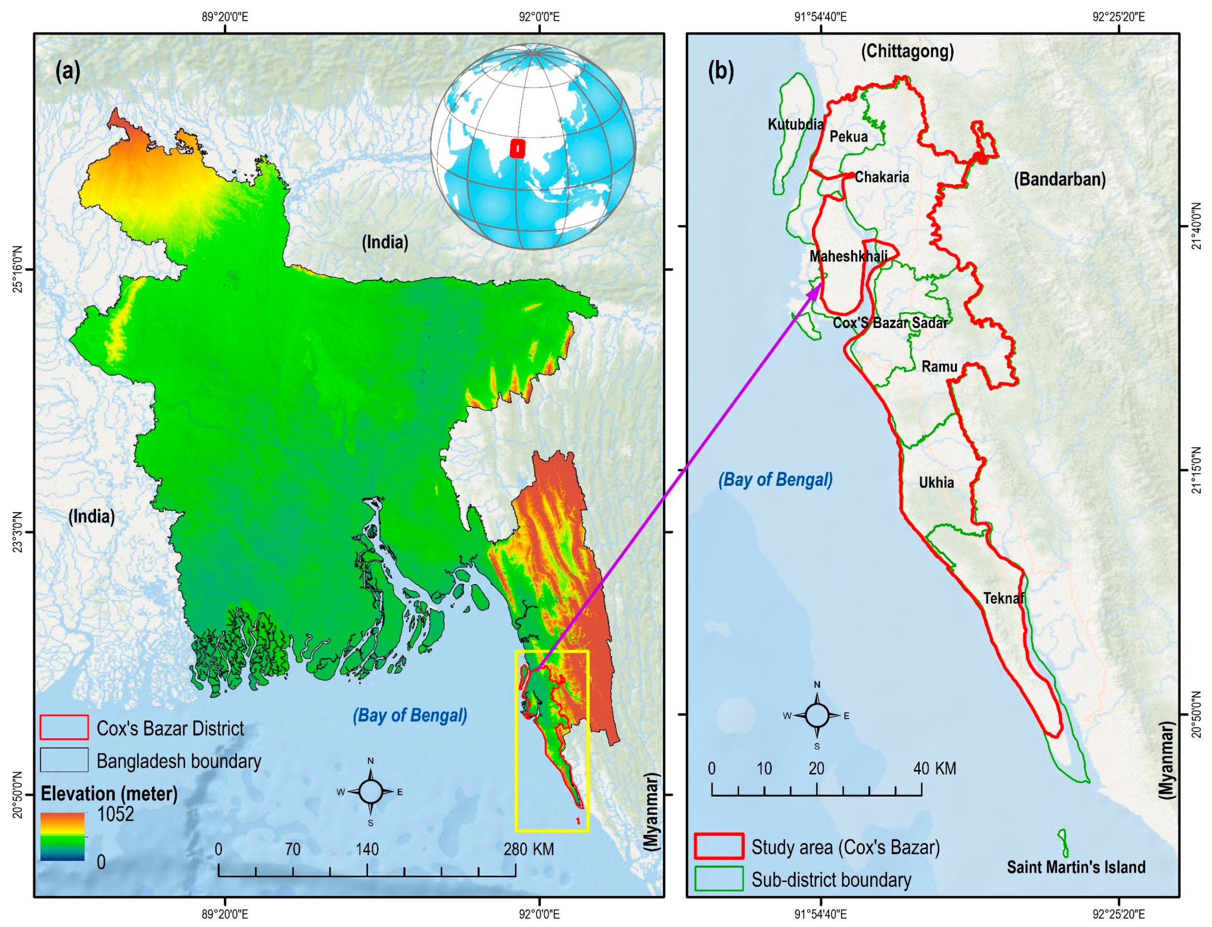
Figure 2.
The process of evaluating spatial agreement among various machine learning technique-based landslide susceptibility maps and optimizing the landslide prediction map. LSM = landslide susceptibility maps; KNN = K-Nearest Neighbor; MLP = Multi-Layer Perceptron; RF = Random Forest; SVM = Support Vector Machine.
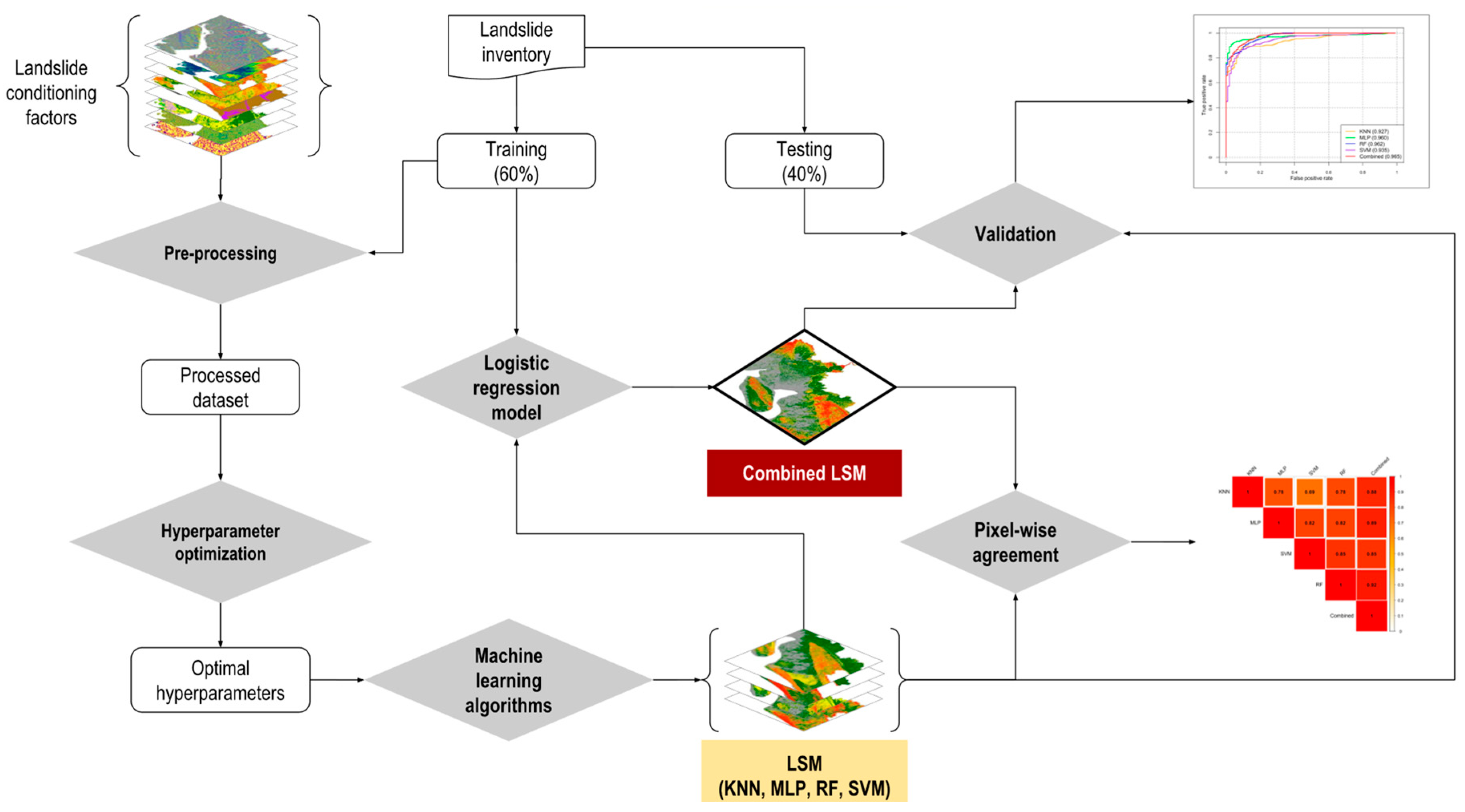
Figure 3.
Landslide inventory map of this study. Data source: [11].
Figure 3.
Landslide inventory map of this study. Data source: [11].
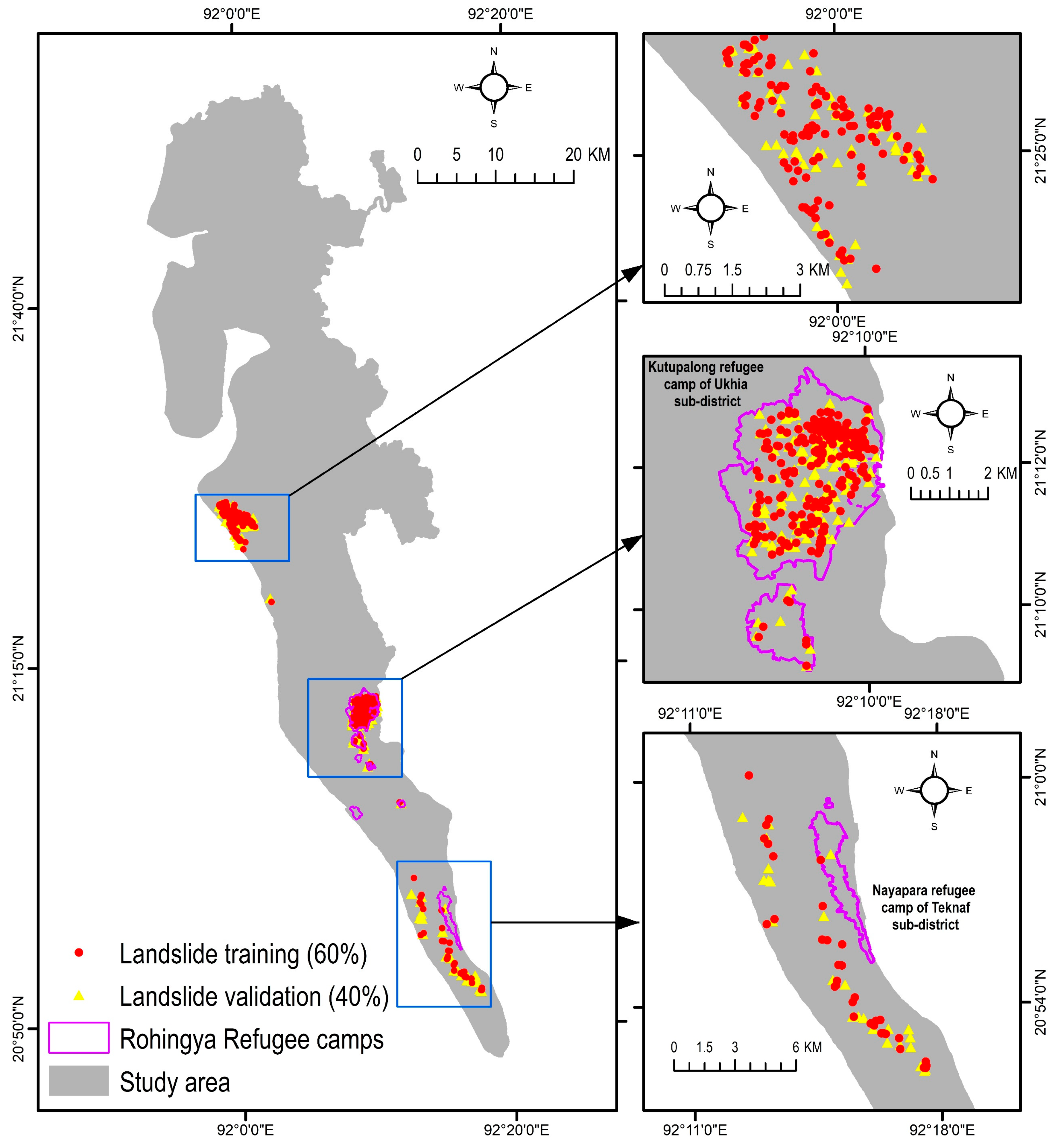
Figure 4.
Landslide conditioning factors. SPI = Stream Power Index. NDVI = Normalized Difference Vegetation Index.
Figure 4.
Landslide conditioning factors. SPI = Stream Power Index. NDVI = Normalized Difference Vegetation Index.
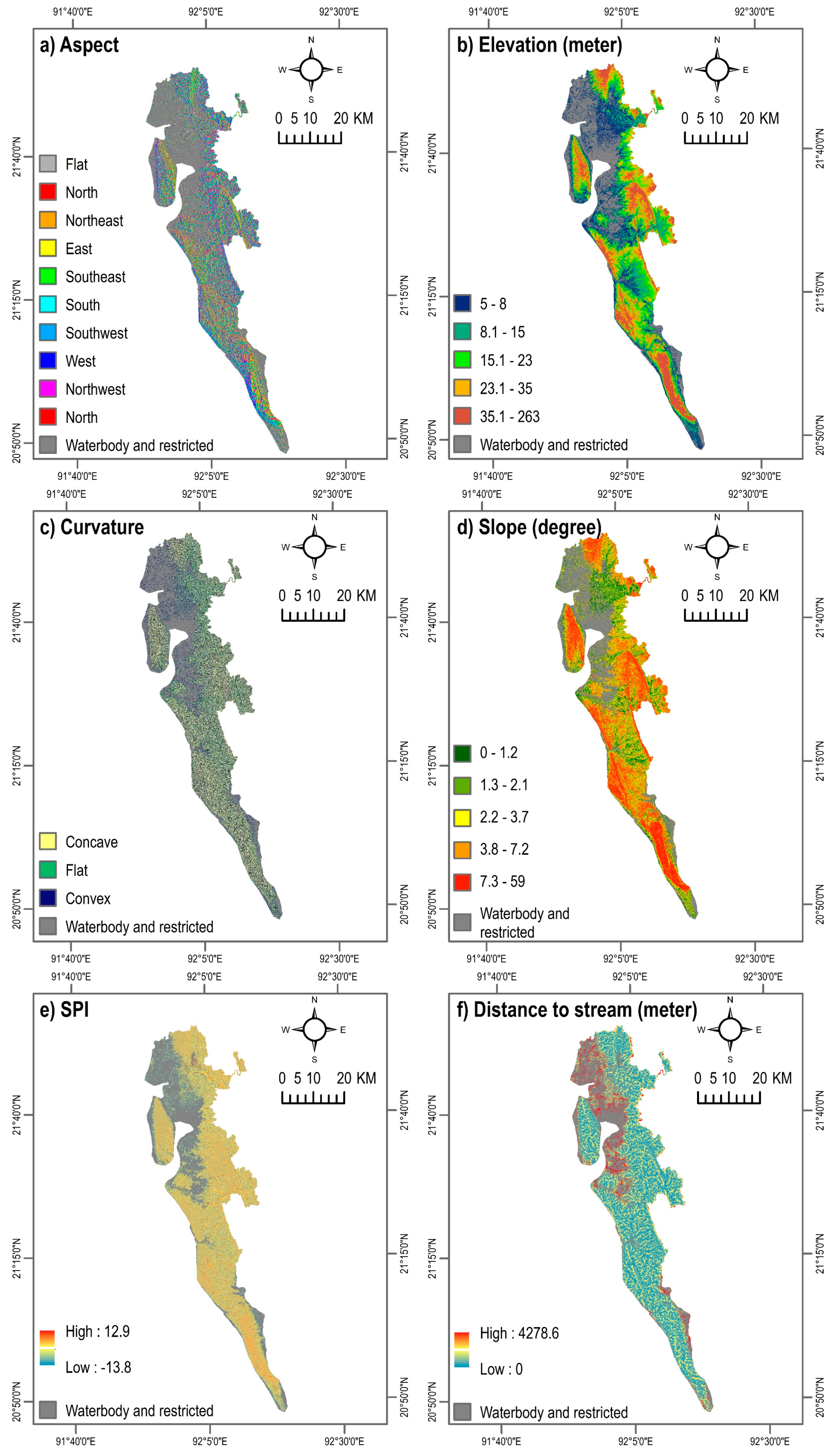

Figure 5.
Landslide susceptibility maps obtained by four machine learning algorithms: (a) K-Nearest Neighbor (KNN), (b) Multi-Layer Perceptron (MLP), (c) Random Forest (RF), and (d) Support Vector Machine (SVM).
Figure 5.
Landslide susceptibility maps obtained by four machine learning algorithms: (a) K-Nearest Neighbor (KNN), (b) Multi-Layer Perceptron (MLP), (c) Random Forest (RF), and (d) Support Vector Machine (SVM).

Figure 6.
Landslide susceptible area obtained using five models: K-Nearest Neighbor (KNN), Multi-Layer Perceptron (MLP), Random Forest (RF), Support Vector Machine (SVM), and combined model. Blue dots indicate the proportion of people exposed to ‘high’ and ‘very high’ susceptible zones.
Figure 6.
Landslide susceptible area obtained using five models: K-Nearest Neighbor (KNN), Multi-Layer Perceptron (MLP), Random Forest (RF), Support Vector Machine (SVM), and combined model. Blue dots indicate the proportion of people exposed to ‘high’ and ‘very high’ susceptible zones.
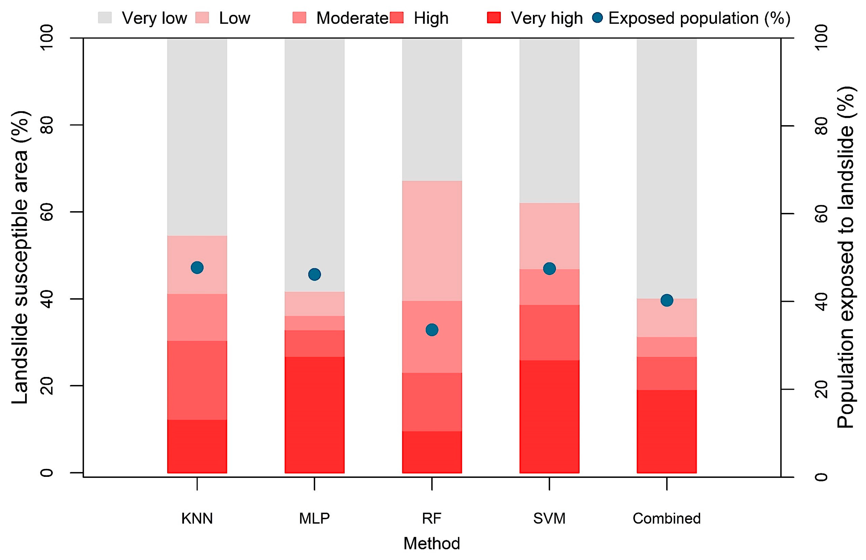
Figure 7.
Receiver operating characteristic (ROC) curves of the five models: K-Nearest Neighbor (KNN), Multi-Layer Perceptron (MLP), Random Forest (RF), Support Vector Machine (SVM), and combined model.
Figure 7.
Receiver operating characteristic (ROC) curves of the five models: K-Nearest Neighbor (KNN), Multi-Layer Perceptron (MLP), Random Forest (RF), Support Vector Machine (SVM), and combined model.

Figure 8.
Correlogram to show the agreement between the five landslide susceptibility models: K-Nearest Neighbor (KNN), Multi-Layer Perceptron (MLP), Random Forest (RF), Support Vector Machine (SVM), and combined model.
Figure 8.
Correlogram to show the agreement between the five landslide susceptibility models: K-Nearest Neighbor (KNN), Multi-Layer Perceptron (MLP), Random Forest (RF), Support Vector Machine (SVM), and combined model.
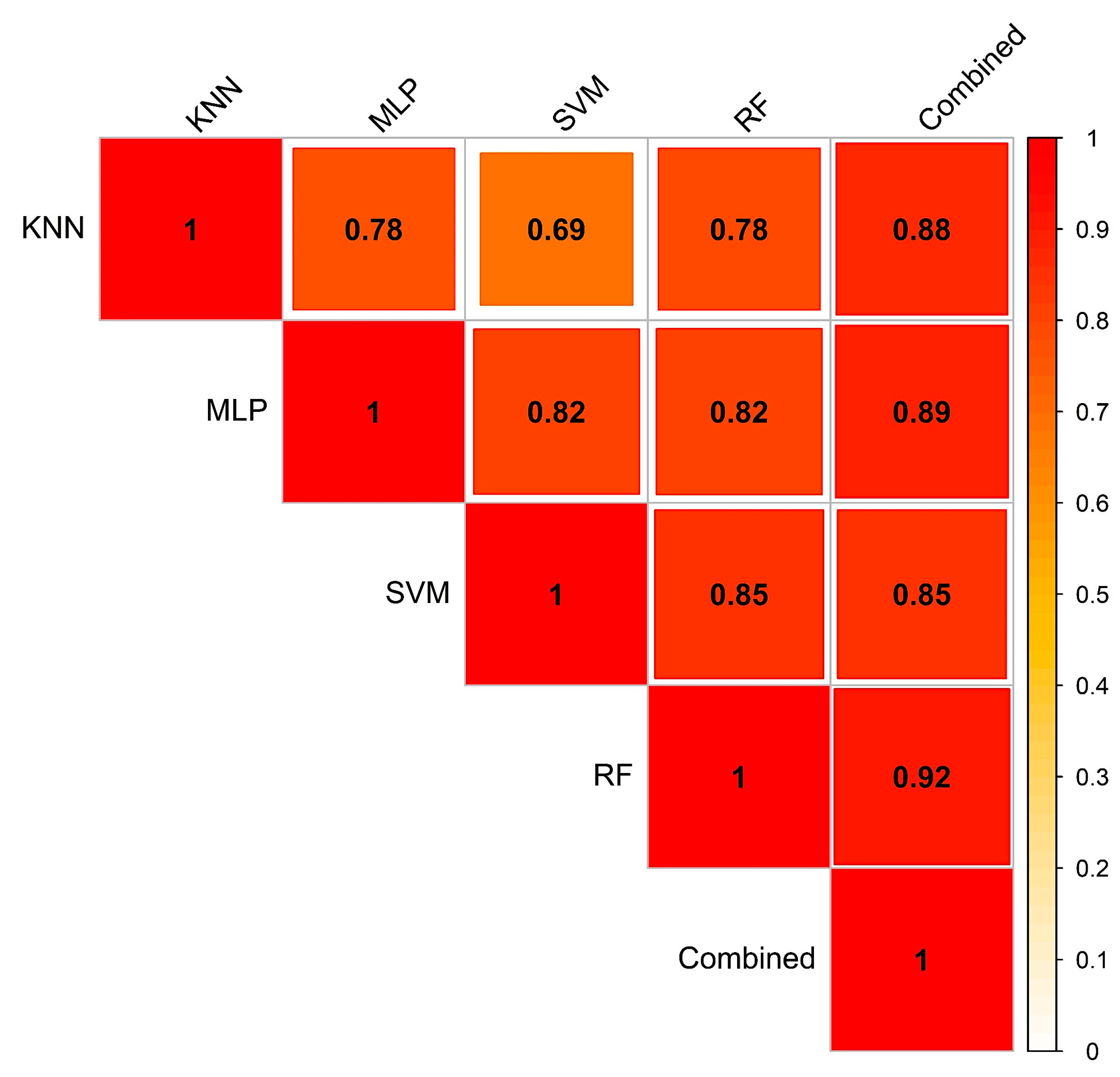
Figure 9.
(a) Combined landslide susceptibility map of Cox’s Bazar district, (b) ratio of landslide susceptible zones (high and very high) in various sub-districts (Upazila), and (c) landslide susceptibility in the Rohingya refugee camps of Ukhia sub-district.
Figure 9.
(a) Combined landslide susceptibility map of Cox’s Bazar district, (b) ratio of landslide susceptible zones (high and very high) in various sub-districts (Upazila), and (c) landslide susceptibility in the Rohingya refugee camps of Ukhia sub-district.


Table 1.
Landslide conditioning factors used in this study.
| No. | Conditioning Factor | Spatial Resolution | Variable Type | Data Source | Variance Inflation Factors (VIF) |
|---|---|---|---|---|---|
| 1 | Aspect | 30 m | Continuous | Estimated from the Digital Elevation Model (DEM) | 1.02 |
| 2 | Elevation | ″ | ″ | DEM [28] | 2.77 |
| 3 | Curvature | ″ | ″ | Estimated from the DEM | 1.57 |
| 4 | Slope | ″ | ″ | ″ | 2.83 |
| 5 | Stream Power Index (SPI) | ″ | ″ | ″ | 1.60 |
| 6 | Distance to stream | ″ | ″ | ″ | 1.15 |
| 7 | Land cover | ″ | Discrete | Landsat Operational Land Imager (OLI) (https://earthengine.google.com) | 1.13 |
| 8 | Normalized difference vegetation index (NDVI) | ″ | Continuous | ″ | 1.24 |
| 9 | Geology | ″ | Discrete | [46] | 1.06 |
| 10 | Soil type | ″ | ″ | [49] | 1.13 |
| 11 | Soil texture | ″ | ″ | ″ | 1.06 |
| 12 | Distance to road | ″ | Continuous | [52] | 1.10 |
Table 2.
Hyperparameters, search range, and optimal values of the machine learning-based landslide susceptibility models.
Table 2.
Hyperparameters, search range, and optimal values of the machine learning-based landslide susceptibility models.
| Classifier | Hyperparameter | Remark | Search Range | Optimal Value |
|---|---|---|---|---|
| K-Nearest Neighbor | Metric | Distance metric to use | Euclidean, Manhattan | Manhattan |
| Number of neighbors | Number of neighbors used for prediction | 3, 5, 11, 19 | 5 | |
| Weights | Weight function used in prediction | Uniform, distance | Distance | |
| Support Vector Machine | C value | Inverse regularization strength | 10−3, 10−2, 10−1, 1, 101, 102, 103 | 103 |
| Kernel | Functions for transforming inputs | Polynomial, radial basis function, sigmoid | Radial basis function | |
| Gamma | Kernel coefficient | 10−3, 10−2,10−1, 1 | 10−3 | |
| Multi-Layer Perceptron | Hidden layer Size | Number of hidden units | 10, 15, 20, 25, 30, 35, 40, 45 | 20 |
| Activation function | Nonlinearity for squeezing output to desired range | Identity, logistic, hyperbolic tangent, rectified linear unit | Rectified linear unit | |
| Learning rate | Specifies if learning rate is constant or variable | Constant, adaptive | Constant | |
| Alpha | L2 penalty/regularization term | 10−4, 10−3, 10−2, 10−1 | 10−4 | |
| Random Forest | Number of estimators | Number of trees in the random forest | 200, 300, 400, 500 | 500 |
| Maximum features | Maximum features to be considered | Auto, square root, logarithm (base = 2) | Auto | |
| Maximum depth | Maximum depth of internal trees | 10, 12, 14, 16, 18, 20, 22, 24, 26, 28 | 10 | |
| Criterion | Function for measuring quality of split | Gini, entropy | Entropy |
Table 3.
Performance evaluation indicators of the machine learning based landslide susceptibility models.
Table 3.
Performance evaluation indicators of the machine learning based landslide susceptibility models.
| Model | Overall Accuracy | Precision | F1-score | Recall | |||
|---|---|---|---|---|---|---|---|
| Non-Landslide | Landslide | Non-Landslide | Landslide | Non-Landslide | Landslide | ||
| KNN | 0.9069 | 0.9227 | 0.9227 | 0.9015 | 0.9015 | 0.8811 | 0.8811 |
| MLP | 0.9545 | 0.9547 | 0.9547 | 0.9528 | 0.9528 | 0.9508 | 0.9508 |
| RF | 0.9663 | 0.9633 | 0.9633 | 0.9652 | 0.9652 | 0.9672 | 0.9672 |
| SVM | 0.9406 | 0.9385 | 0.9385 | 0.9385 | 0.9385 | 0.9385 | 0.9385 |
Table 4.
Outcomes of the logistic regression model.
| Variables (Landslide Susceptibility Models) | Coefficient | p-Value |
|---|---|---|
| Intercept | −5.84 | <2.2e−16 *** |
| KNN | 0.64 | 0.34 |
| MLP | 3.52 | 2.67e−09 *** |
| RF | 5.01 | 8.449e−09 *** |
| SVM | 2.02 | 0.01205 * |
| Significance codes: 0 ‘***’ 0.001 ‘**’ 0.01 ‘*’ 0.05 ‘▪’ 0.1 ‘ ’ 1. Coefficient of determination R2: 0.80 Log-Likelihood: −178.42 | ||
© 2020 by the authors. Licensee MDPI, Basel, Switzerland. This article is an open access article distributed under the terms and conditions of the Creative Commons Attribution (CC BY) license (http://creativecommons.org/licenses/by/4.0/).
Share and Cite
MDPI and ACS Style
Adnan, M.S.G.; Rahman, M.S.; Ahmed, N.; Ahmed, B.; Rabbi, M.F.; Rahman, R.M. Improving Spatial Agreement in Machine Learning-Based Landslide Susceptibility Mapping. Remote Sens. 2020, 12, 3347. https://doi.org/10.3390/rs12203347
AMA Style
Adnan MSG, Rahman MS, Ahmed N, Ahmed B, Rabbi MF, Rahman RM. Improving Spatial Agreement in Machine Learning-Based Landslide Susceptibility Mapping. Remote Sensing. 2020; 12(20):3347. https://doi.org/10.3390/rs12203347
Chicago/Turabian StyleAdnan, Mohammed Sarfaraz Gani, Md Salman Rahman, Nahian Ahmed, Bayes Ahmed, Md. Fazleh Rabbi, and Rashedur M. Rahman. 2020. "Improving Spatial Agreement in Machine Learning-Based Landslide Susceptibility Mapping" Remote Sensing 12, no. 20: 3347. https://doi.org/10.3390/rs12203347
Note that from the first issue of 2016, this journal uses article numbers instead of page numbers. See further details here.