Article

Hyperspectral Inversion of Phragmites Communis Carbon, Nitrogen, and Phosphorus Stoichiometry Using Three Models

1
Institute of Wetland Research, Chinese Academy of Forestry, Beijing Key Laboratory of Wetland Services and Restoration, Beijing 100091, China
2
Beijing Hanshiqiao National Wetland Ecosystem Research Station, Beijing 101399, China
*
Author to whom correspondence should be addressed.
Remote Sens. 2020, 12(12), 1998; https://doi.org/10.3390/rs12121998
Submission received: 25 May 2020 / Revised: 19 June 2020 / Accepted: 21 June 2020 / Published: 22 June 2020
(This article belongs to the Section Remote Sensing in Agriculture and Vegetation)

Abstract

:
Studying the stoichiometric characteristics of plant C, N, and P is an effective way of understanding plant survival and adaptation strategies. In this study, 60 fixed plots and 120 random plots were set up in a reed-swamp wetland, and the canopy spectral data were collected in order to analyze the stoichiometric characteristics of C, N, and P across all four seasons. Three machine models (random forest, RF; support vector machine, SVM; and back propagation neural network, BPNN) were used to study the stoichiometric characteristics of these elements via hyperspectral inversion. The results showed significant differences in these characteristics across seasons. The RF model had the highest prediction accuracy concerning the stoichiometric properties of C, N, and P. The R2 of the four-season models was greater than 0.88, 0.95, 0.97, and 0.92, respectively. According to the root mean square error (RMSE) results, the model error of total C (TC) inversion is the smallest, and that of C/N inversion is the largest. The SVM yielded poor predictive results for the stoichiometric properties of C, N, and P. The R2 of the four-season models was greater than 0.82, 0.81, 0.81, and 0.70, respectively. According to RMSE results, the model error of TC inversion is the smallest, and that of C/P inversion is the largest. The BPNN yielded high stoichiometric prediction accuracy. The R2 of the four-season models was greater than 0.87, 0.96, 0.84, and 0.90, respectively. According to RMSE results, the model error of TC inversion is the smallest, and that of C/P inversion is the largest. The accuracy and stability of the results were verified by comprehensive analysis. The RF model showed the greatest prediction stability, followed by the BPNN and then the SVM models. The results indicate that the accuracy and stability of the RF model were the highest. Hyperspectral data can be used to accurately invert the stoichiometric characteristics of C, N, and P in wetland plants. It provides a scientific basis for the long-term dynamic monitoring of plant stoichiometry through hyperspectral data in the future.

Graphical Abstract

1. Introduction

All living organisms are composed of multiple chemical elements, with the three main ones being C, N, and P. The balance of elements has an important influence on biological production, and nutrient cycling [1]. Many key characteristics of organisms and ecosystems can be determined by the dynamic ratio of these elements [2]. Such an approach, known as “ecological stoichiometry,” studies the elemental components of organisms, particularly C, N, and P [3]. Ecological chemometrics is a comprehensive method of studying the coupling relationship of C, N, and P in ecosystem processes by using the balance relationship of the multiple chemical elements in those processes [2,3]. The core challenge of chemometrics is to reveal the impact of differences in the compositions of biological elements on ecological functions. Such an understanding can successfully link different research disciplines on various scales, from molecules to organisms, from ecosystems to the biosphere [4,5,6]. In 1958, chemometrics was introduced into ecosystem research by Redfield, who mainly studied the cycles of C, N, and P in ecosystems [7]. Elser et al. [8] put forward the concept of ecological chemometrics for the first time. Ecochemometrics has proved valuable in promoting understanding of the various connections between trophic interactions and nutrient cycles [9,10,11].
As essential nutrients for plant growth and development, C, N, and P play important roles in plant growth, and in various closely interrelated physiological regulatory functions [12,13,14]. For example, N and P are the two most important limiting elements of vegetation growth. The N/P ratio of plants is relatively constant on a global scale [15]. At the species community level, N/P ratio is related to individual growth rate, and even more so to community structure [16,17]. Studying the stoichiometric characteristics of C, N, and P provides an effective means of understanding the survival and adaptation strategies of plants [2]. Therefore, accurate evaluation of plant growth is dependent on the development of methods by which to rapidly and nondestructively monitor stoichiometric characteristics of plants [18,19]. However, the traditional stoichiometric monitoring method based on laboratory analysis is harmful to plants and unsuitable for large-scale applications. In particular, the wetland environment poses some challenges to sample collection, making it difficult to achieve long-term dynamic monitoring [20]. Remote sensing has become an alternative monitoring method in recent years by providing an important means of monitoring plant growth and quantifying plant biophysical and biochemical characteristics [21,22,23]. Specifically, because the structure of plant components are directly affected by the C, N, and P, the content of these elements directly affects the spectral reflectance of individual leaves, as well as reflectance at the canopy level [24]. Hyperspectral remote sensing technology can be applied to the real-time monitoring of phytochemistry.
Many scholars have carried out extensive research on hyperspectral inversion of vegetation elemental composition and have found variations in the spectral bands corresponding to different elemental abundances [25]. Further, different models can vary in their inversion effects on vegetation elements. Some studies have shown that the vegetation index model can effectively predict the N content of rice, soybean, corn, and other crops; the red-edge parameter model can effectively predict the N and P contents of rice; and machine models, such as the random forest (RF), support vector machine (SVM), and back propagation neural network (BPNN) have high accuracy and stability when applied to the C, N, and P contents of vegetation [26,27,28,29,30,31]. The elemental composition of vegetation changes with different growth stages, so the monitoring and research of vegetation elements should be carried out in different seasons. At present, most research is focused on crops, with very few studies considering wetland plants in different growing seasons. Moreover, current research tends to focus primarily on the direct prediction of element content; more research is needed to determine whether this approach can be applied to stoichiometric prediction.
The study area was Beijing Hanshiqiao Wetland Nature Reserve. Sample collection was carried out during all four seasons in one year. After collecting the reflectance spectrum data and the C, N, and P stoichiometric characteristics of the reed canopy, models were established using RF, SVM, and BPNN models. The accuracy and stability of each model were compared and analyzed for different seasons and for different inversions of the hyperspectral data. The aim was to provide a scientific basis for estimating and dynamically monitoring reed stoichiometry by hyperspectral data in different seasons without causing damage to the plants.

2. Materials and Methods
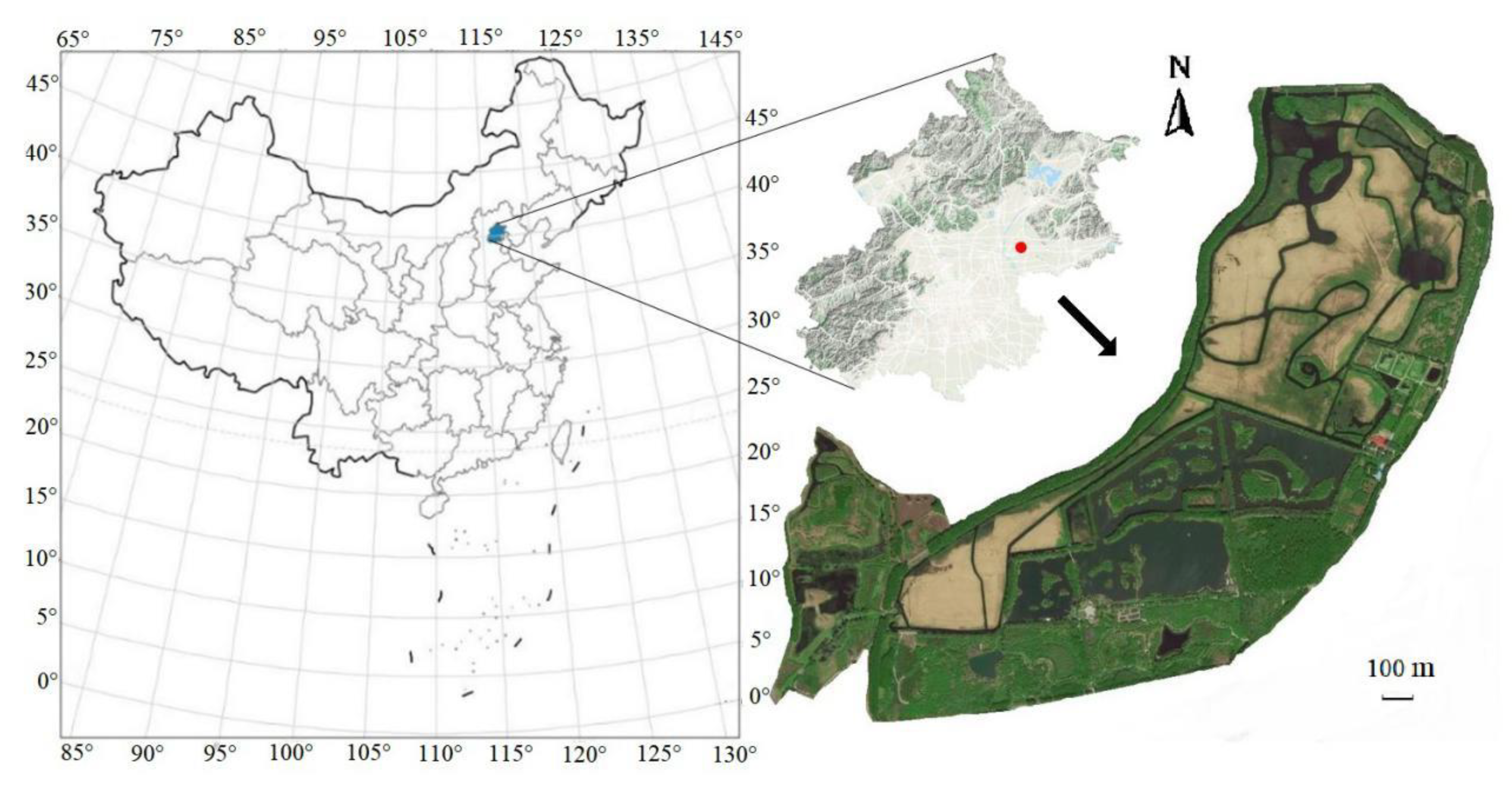
2.1. Study Area

The study was conducted in Beijing Hanshiqiao Wetland Nature Reserve (40°07′N and 116°48′E) located in Shunyi District, Beijing (Figure 1). It is a swamp wetland on the outskirts of Beijing covering a total area of 1900 ha, where management focuses on protecting reed (Phragmites communis) swamp and wild animals. It is part of the Chaobai River system, with the Caijia River as its main water source. The area has a warm temperate semi-humid monsoon climate, with an average annual temperature of 11.9 °C and average annual precipitation of 603 mm [32]. Precipitation mainly occurs from July to August. Reeds in our wetland study area are growing in 5–30 cm of water. During the sampling period, the vegetation coverage is 80–90% in spring and 85–95% in the other three seasons.

2.2. Data Collection

Sampling was conducted in each season in 2018 (in April, July, October, and December), with 90 samples collected each season. In order to ensure the comparability of samples from different seasons, a total of 60 fixed plots were set up in the upstream, middle, and downstream regions of the reserve, and the remaining sampling points were randomly distributed, for a total of 120 random plots over the study period. The size of each quadrat was 1 m × 1 m.
Spectral data of the reed canopy were collected using ASD FieldSpec 4 spectroradiometer (ASD, Analytical Spectral Devices, Inc., Boulder, CO, USA), in the wavelength range of 350–2500 nm. A 5-m fiber optic cable was attached, and the height of the support rod was adjusted to ensure that the spectral probe maintained a distance of 1 m from the reed canopy in the quadrat. Data collection was conducted between 10:00 and 14:00 local time (China Standard Time, GMT+8). At this time, the solar elevation angle was greater than 45°, which ensures good lighting conditions. The spectrum was corrected using a reference panel before each sample was collected. Ten spectral datasets were collected and averaged as one spectral reading for each sampling point. In order to ensure accurate inversion of the reed stoichiometry, the spectral bands affected by water-vapor absorption were removed.
Three reeds were harvested from each quadrat, treated in a drying box at 105 °C for 30 min to halt oxidation, and then dried at 80 °C until a constant mass was reached. The dried reeds were crushed and sieved. Plant C and N were measured using an elemental analyzer (vario EL III, CHNOS elemental analyzer, Elementar Analysensysteme GmbH, Germany), and plant P content was measured using an ultraviolet-visible spectrophotometer (UV-2550, UV-Visible spectrophotometer, Shimadzu, Japan).

2.3. Methods

Due to the large number of bands, strong correlations, and data redundancies that are characteristic of hyperspectral data, related calculations are complex. Principal component analysis (PCA) was applied to reduce the dimensionality of the hyperspectral data by compressing many interrelated variables into a few uncorrelated new component variables, each containing a large amount of information from the original data [33]. Taking the principal component after PCA as the independent variable, the next step was to build the prediction model of reed C, N, and P stoichiometry. Each season, 90 samples were randomly assigned to two groups: one group was used for model building, and the other was used for model validation. Using Weka 3.8 software, three models (RF, SVM, and BPNN) were selected to invert hyperspectral data in order to analyze the reed C, N, and P stoichiometry. The accuracy and stability of the models were evaluated by the determination coefficient (R2) and root mean square error (RMSE).
The RF is an integrated learning algorithm used for classification and regression. It is constructed by combining the results of various decision trees and bagging the original dataset to select samples [34]. Each decision tree determines the class tag predictor (termed “vote”) for the new instance. Then, the votes generated by various decision trees are calculated, and the class with the majority of votes is assumed to “win”; thus, the new instance is predicted [35]. In this study, using Weka software, a random subspace is first constructed and then the operation is implemented based on the J48 (C4.5) algorithm. The parameters for numIterations, seed, confidence factor, and numFolds are 10, 1, 0.25, and 3, respectively.
The SVM is a very popular machine-learning technology. This supervised learning model contains related learning algorithms, which are used to analyze, classify, and conduct regression analysis on the supplied data [36]. The sample is set with input and output variables; an optimal function to minimize the expected loss is determined; and the balance between the looseness of the function and the value is adjusted. After learning the sample set, the regression prediction equation is constructed [37]. In this study, Weka software using the Gaussian kernel function is used as the kernel function in the SVM model with the kernel size set to 17.
A BPNN is a multilayer feed-forward neural network trained according to the error back-propagation algorithm. It is a machine model that takes the square of network error as an objective function and uses the gradient descent method to calculate the minimum value of the objective function [38]. This model uses powerful data recognition and simulation abilities to model nonlinear systems. The BPNN is trained using the input and output data until it can express the unknown black box function, and then the trained network is used to predict the system output. In this study, Weka software was based on the multilayer perceptron algorithm, the sigmoid function is used as the transfer function and the number of neurons in the hidden layer is set to 10.

3. Results

3.1. Stoichiometric Characteristics of Reed

The stoichiometric characteristics of reed C, N, and P were significantly different across seasons, but there were low error bars for all samples of reed collected within the same season (Figure 2). This shows that the stoichiometric characteristics of reed are unique in different growing seasons. The average value of total N (TN) is highest in summer and lowest in winter. The values are 36.81 and 5.25 mg/g, respectively. The average value of total P (TP) is highest in spring and lowest in winter. The values are 3.79 and 0.40 mg/g, respectively. The average value of total C (TC) is both highest and lowest in summer. The values are 458.49 and 392.45 mg/g, respectively. The average value of C/N is highest in winter and lowest in summer; the values are 84.31 and 12.19, respectively. The average value of N/P is highest in summer and lowest in spring; the values are 15.90 and 6.70, respectively. The average value of C/P is highest in winter and lowest in spring. The values are 1088.28 and 111.37, respectively. The values and ranges of specific stoichiometric characteristics for reed C, N, and P in each of the four seasons are summarized in Table 1.

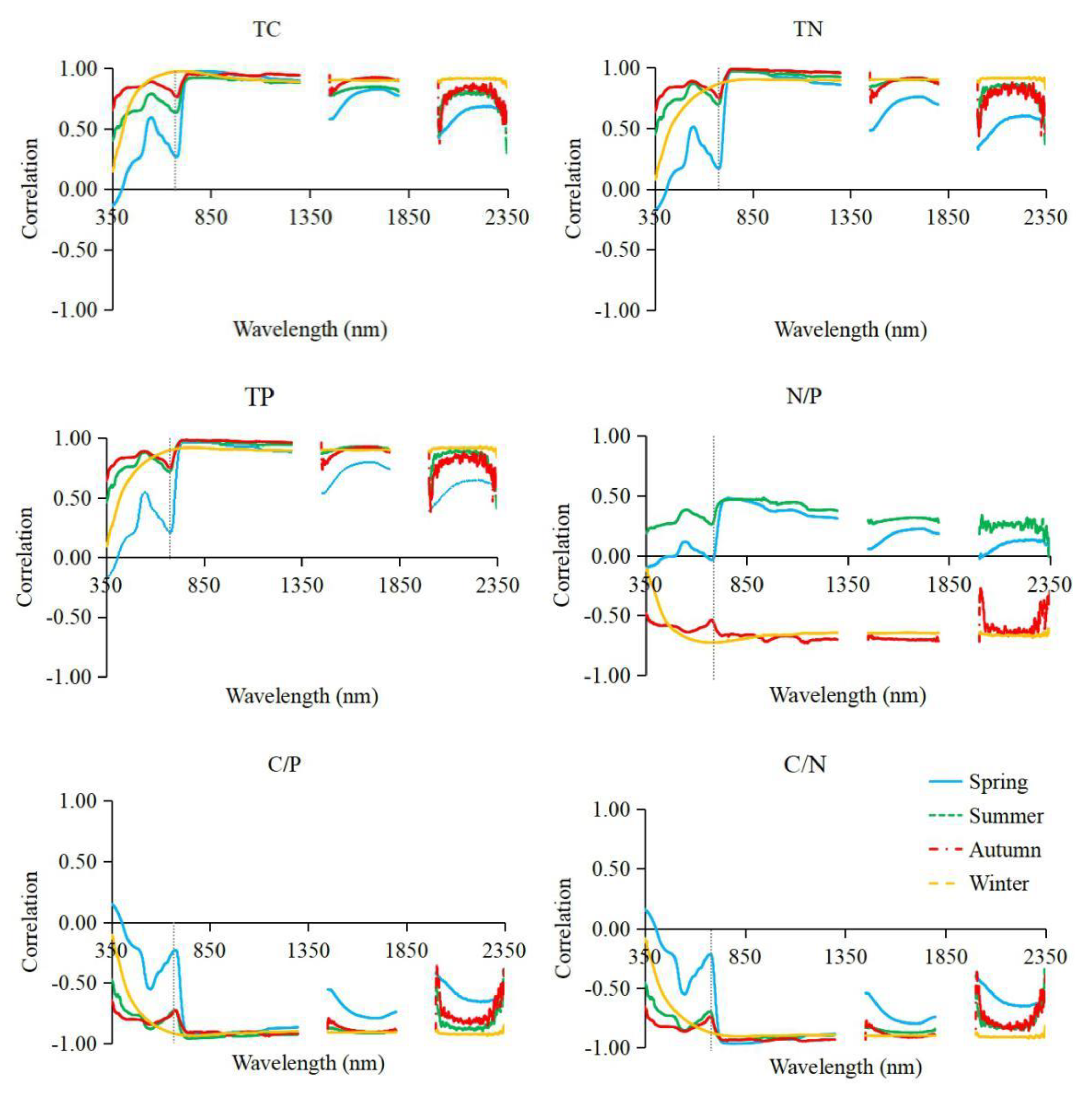
3.2. Correlation Analysis

The results show that the correlation between winter spectral reflectance and plant stoichiometry is markedly different from that of the other seasons. In winter, TC, TN, and TP all show a large positive correlation at 650 nm, while C/N, N/P, and C/P all show a large negative correlation at 650 nm (Figure 3). In other seasons, the TC, TN, TP, and spectral reflectance correlations of vegetation are in the following order: autumn > summer > spring. The optimal correlation band positions and values of TC, TN, TP, and spectral reflectance are similar across all four seasons. The C/P and C/N values are negatively correlated with spectral reflectance for all four seasons, while the N/P value is positively correlated with spectral reflectance in spring and summer, and negatively correlated in autumn and winter. The overall correlation between N/P and spectral reflectance (Figure S1) is significantly lower than the other five stoichiometric parameters assessed.

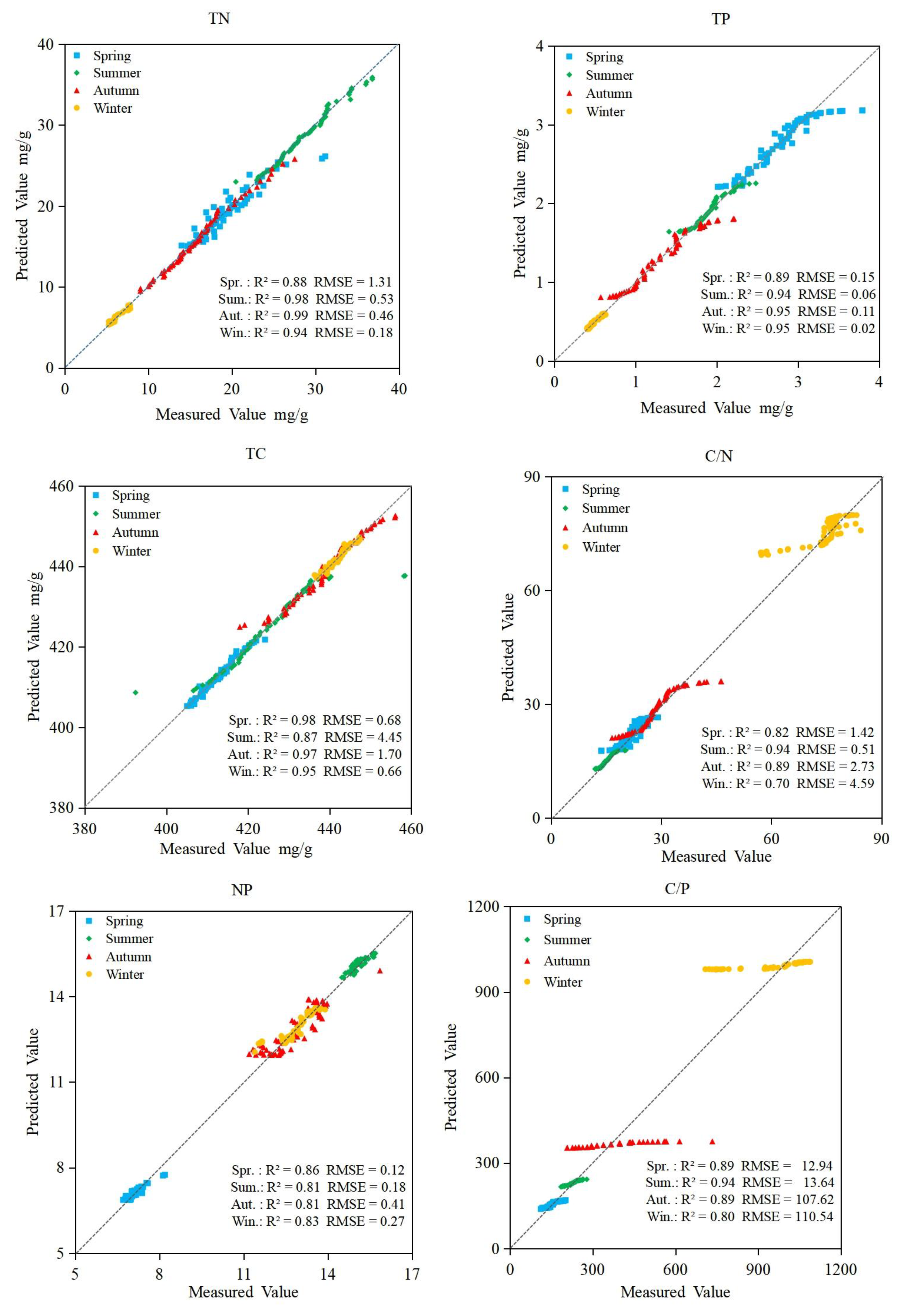
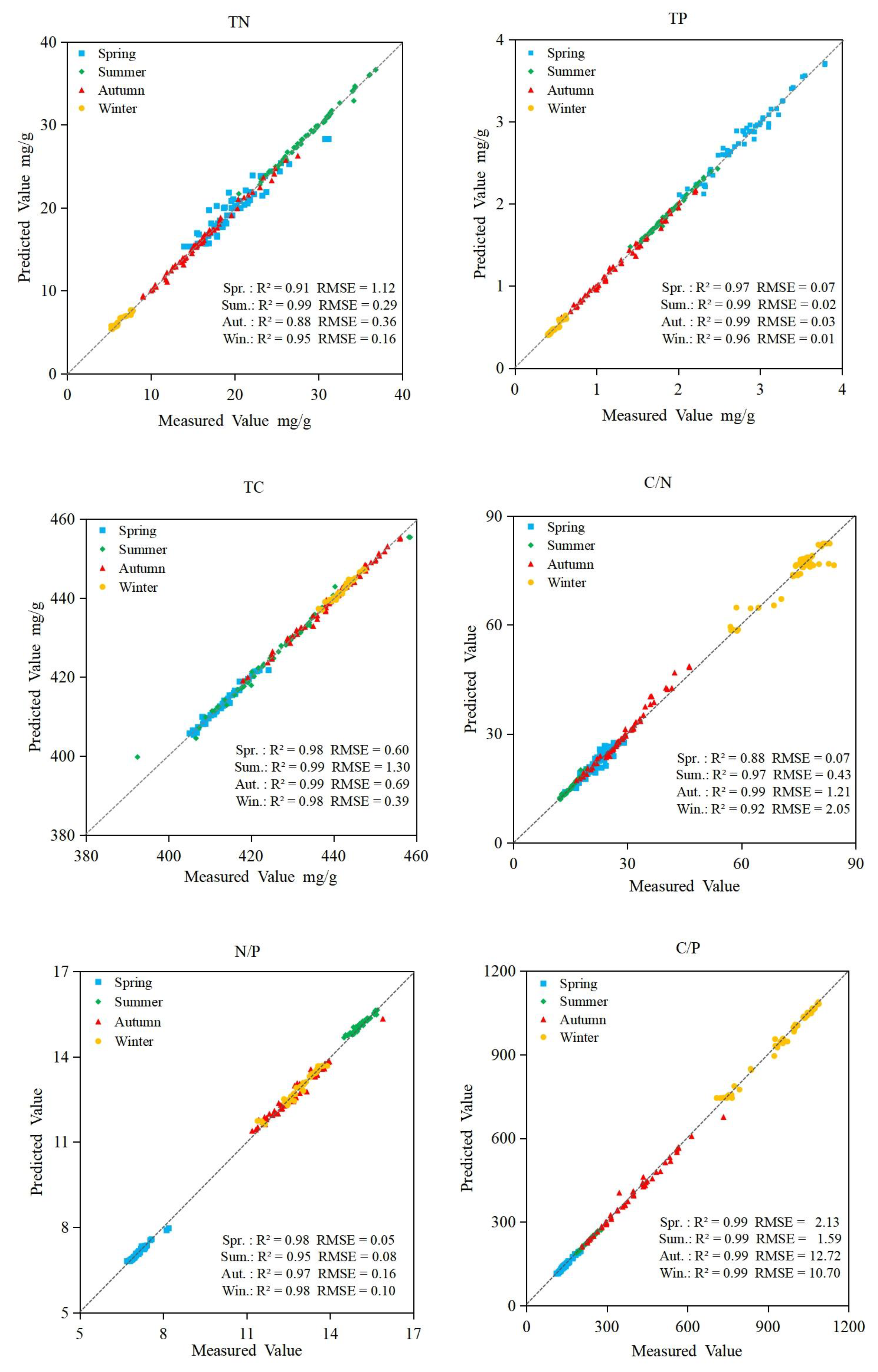
3.3. Random Forest Regression Models

The RF model has good prediction accuracy concerning the stoichiometric properties of C, N, and P. Prediction accuracy decreases across seasons in the order of autumn, summer, winter, and spring (Figure 4). The R2 for autumn is greater than 0.97, and that for summer is greater than 0.95. The R2 of C/N is lower in winter, with a value of 0.92. The R2 values for TN and C/N are lower in spring than for the other seasons (0.91 and 0.88, respectively), and the prediction error is also greater than that for other seasons. The prediction accuracy is highest for C/P, with an R2 of 0.99 for all four seasons. The R2 values for TC and TP are also greater than 0.96. The RMSE values of the inversion models of TC and TN in spring and TP in summer are higher than those of other seasons; those of C/N, C/P, and N/P in autumn and winter are higher than those of spring and summer. The prediction accuracy of the random forest model is slightly higher for TN, TP, and TC than for C/N, N/P, and C/P.

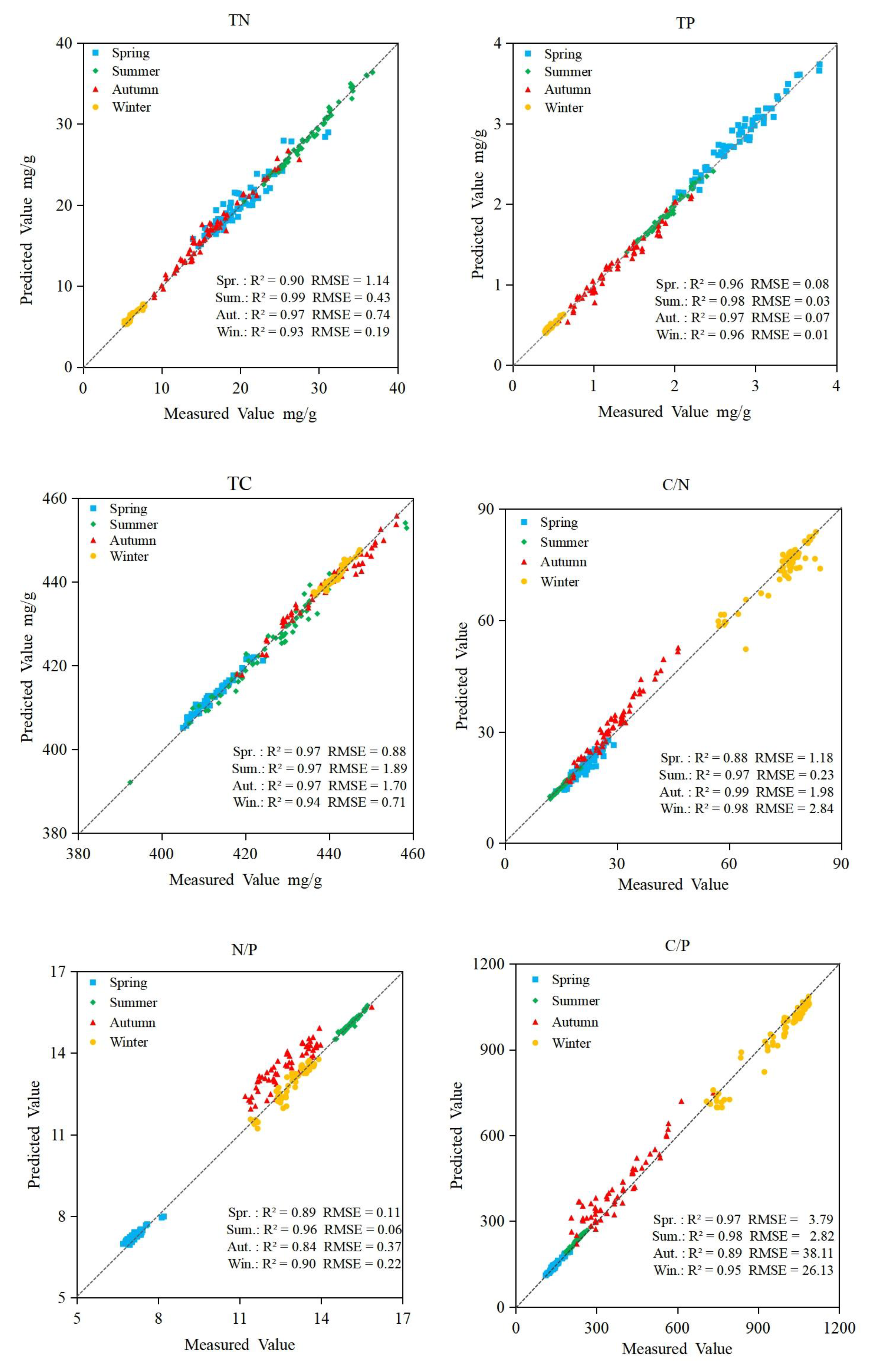
3.4. Support Vector Machine Regression Models

The SVM yielded poor predictive results for the stoichiometric properties of C, N, and P. Prediction accuracy decreases across the seasons in the order of autumn, winter, summer, and spring (Figure 5). In spring, the R2 value for TC is 0.98, and that of the other stoichiometric parameters is less than 0.89. According to RMSE results, the model error of TN inversion in spring is the largest. In summer, the R2 value of N/P is 0.81. According to the results of RMSE, the error of the summer model is the smallest. In autumn, the R2 value for N/P is only 0.81, while that of the other stoichiometric parameters is greater than 0.89. The winter R2 values for C/N, C/P, and N/P are 0.70, 0.81, and 0.83, respectively. According to the results of RMSE in autumn and winter, the inversion errors of the model to C/N, C/P, and N/P are high. From the perspective of chemometrics, the prediction accuracy of the SVM model is highest for TC, with an R2 that is greater than 0.87. The prediction accuracy of the SVM model for TN, TP, and TC is greater than for C/N, N/P, and C/P, as the R2 values of the former group are mostly larger than 0.94, whereas those of the latter group are mostly less than 0.89.

3.5. BP Neural Network Regression Models

The BPNN yielded high stoichiometric prediction accuracy. However, the prediction accuracy of the BPNN differs from that of the other two models when comparing seasonal results. Prediction accuracy decreases across the seasons in the order of summer, winter, spring, and autumn (Figure 6). The R2 of each stoichiometric parameter is greater than 0.96 for summer, and that for winter is greater than 0.90. The prediction accuracy for N/P is low for spring and autumn, with R2 values of 0.87 and 0.84, respectively. The R2 values of TN, TP, and TC were greater than 0.96 for all four seasons. The RMSE results of stoichiometric inversion models in different seasons were similar to the trends of the other models, with TC, TN and TP errors less than C/N, C/P and N/P. The prediction accuracy of the BPNN is better for TN, TP, and TC than for C/N, N/P, and C/P.

3.6. Accuracy of Prediction Models

The remaining one-third of the data was used for validation of the above built models. The accuracy and stability of the results were verified by comprehensive analysis, the RF model showed the greatest prediction stability, followed by the BPNN, and then the SVM model. For the RF model, the inversion stability of C/N is highest, followed by TN and N/P, and the inversion stability of summer TC and winter C/N require improvement.
The spring R2 values for all stoichiometric characteristics of C, N, and P are greater than 0.86 in all models. The R2 values produced by the SVM for summer TC and N/P are only 0.83 and 0.64, and that of winter TP is only 0.79. The overall prediction accuracy for N/P is poor for all four seasons under this model. The BPNN showed poor predictive power regarding autumn TC and N/P, with R2 values of only 0.86 and 0.84, respectively. Additionally, the R2 for winter TP is only 0.89 (Table 2).
In order to attain identical contrast in model errors across different seasons, the RMSE and the sample average values were processed as proportions. The seasons with both the largest and smallest errors are the same for identical stoichiometric characteristics under the different models. The errors of the three models for TC prediction are all less than 0.5%, except for the summer SVM model, which is 1.04%.

4. Discussion

Plants obtain C, which forms the carbon skeleton that is the basis of organic compounds, from CO2 in the air and water-soluble organic C in the soil. As C is abundant in reed-swamp wetlands, the TC of the reeds is stable across all four seasons. The demand for P is greater in early plant growth stages than in later ones, leading to a gradual reduction of reed TP with seasonal changes. Studies have shown that N is a limiting factor when the N/P ratio is less than 8 [39]. Our results indicate that vegetative growth may be limited in spring by the total N content. As summer is the rainy season in the study area, the N/P ratio of reeds is higher in this season than in the others. Plant C/N reflects plant nutrient utilization efficiency. Because the reeds stop growing in winter, the C/N is 3–4 times higher at this time than in the other three seasons; conversely, during the summer season of vigorous growth, the C/N is the lowest. When analyzing the correlation between phytochemical characteristics and spectral reflectance, the correlation between winter and the other three seasons is significantly different. This may be due to a change in spectral reflectance caused by the withering of vegetation in winter.
The larger the vegetation coverage, the less the spectral characteristic is affected by the underlying surface [40]. The reason that the precision of the stoichiometry inversion model for spring C, N, and P is lower than those of the summer and autumn models may be the lower vegetation coverage in spring. With increasing leaf age, the mesophyll interspace increases. In addition, when the reeds flower in autumn, the vegetation structure becomes more complex, thus increasing the spectral reflectance and noise of the autumn vegetation canopy [40] and reducing the precision of the autumn C, N, and P stoichiometry inversion models.
The RF model has the best inversion effect on wetland plant stoichiometry, and its autumn model R2 is the highest. The strongest correlation between stoichiometry and spectral reflectance was obtained for autumn data. This may be because vegetation growth is maximal in autumn, and the greater vegetation coverage reduces the environmental background interference on spectral data. In addition, the range of sample values is relatively large for autumn, which ensures a more comprehensive range of data. The RF model is good at dealing with nonlinear multiple compound regression problems, easy to improve performance, not easy to overfit, efficient and fast when processing large data sets, and interpretable to the results [41], and is suitable for inverting the stoichiometric characteristics of wetland plants.
The SVM model has high generalization ability and has advantages in solving small sample model inversions, but the model is particularly sensitive to the parameters selected [42,43]. In the present study, the inversion accuracy of the SVM model for TC, TN, and TP is slightly lower than that of the other two models in spring and summer. However, the inversion accuracy for C/N, N/P, and C/P is particularly poor. Therefore, when solving the inversion of small sample plant stoichiometric characteristics in the future, we must select the appropriate kernel function according to the data characteristics.
The BPNN model also has problems with its high inversion accuracy of TC, TN, and TP, and reduced accuracy of C/N, N/P, and C/P inversion. However, its inversion accuracy for C/N, N/P, and C/P is much higher than that of the SVM model. The model R2 for C/N, N/P, and C/P inversion is higher than 0.90, 0.84, and 0.89, respectively. This may be because the BPNN model has overfitting in the process of retrieving the C/N, N/P, and C/P of wetland plants. The R2 of each stoichiometric parameter is greater than 0.96 for summer and greater than 0.90 for winter. This may be because the model tends toward the local minimum.
The modeling results of the prediction model verification are basically consistent with those of the three models. The seasons with both the largest and smallest errors are the same for identical stoichiometric characteristics under the different models. This is related to the range and distribution of sample values. Therefore, in addition to the differences between models, the growth characteristics of vegetation also have a great impact on the accuracy of the model.

5. Conclusions

Based on the stoichiometric characteristics of wetland plant C, N, and P in different seasons, we selected three machine models for hyperspectral inversion. The accuracy of the model is verified. The results allow us to draw the following conclusions:
Hyperspectral data can be used to accurately invert the stoichiometric characteristics of C, N, and P in wetland plants (reed).
All models tested showed higher prediction accuracy for TC, TN, and TP than for C/N, N/P, and C/P.
Of the three models tested, the accuracy and stability of RF are the highest. Within this model, the prediction accuracy and stability are the highest for summer.
This study is a preliminary exploration of the hyperspectral inversion of wetland stoichiometric characteristics in different seasons. It provides a scientific basis for the long-term dynamic monitoring of plant stoichiometry through hyperspectral data in the future.

Supplementary Materials

The following are available online at https://www.mdpi.com/2072-4292/12/12/1998/s1, Figure S1: The reed original spectral reflectance in four seasons.

Author Contributions

Conceptualization, L.C. and W.L.; methodology, Z.D. and W.L.; software, X.Z. (Xinsheng Zhao) and Z.L.; validation, X.Z. (Xueyan Zuo), X.Z. (Xinsheng Zhao), and Z.L.; formal analysis, X.P.; investigation, X.Z. (Xueyan Zuo) and Z.D.; resources, X.P.; data curation, Z.D.; writing—original draft preparation, Z.D., Z.L., and X.Z. (Xueyan Zuo); writing—review and editing, L.C., Y.L., and W.L.; supervision, C.L., J.L., and Y.L.; project administration, W.L.; funding acquisition, W.L. All authors have read and agreed to the published version of the manuscript.

Funding

This research was funded by the China’s special fund for basic scientific research business of central public research institutes (grant no. CAFYBB2017MA028).

Acknowledgments

The authors would like to thank Zhangjie Cai, Yunxi Lu, and Yang Cai for helping us conduct experiments in the field. Thank you also to Ying Guo for her guidance on data analysis software operation.

Conflicts of Interest

The authors declare no conflict of interest.

References

  1. Elser, J.J. Biological Stoichiometry: A Chemical Bridge between Ecosystem Ecology and Evolutionary Biology. Am. Nat. 2006, 168, S25–S35. [Google Scholar] [CrossRef]
  2. Sterner, R.W.; Elser, J.J. Ecological Stoichiometry: The Biology of Elements from Molecules to the Biosphere; Princeton University Press: Princeton, NJ, USA, 2002. [Google Scholar]
  3. Reichert, P.; Schuwirth, N. A generic framework for deriving process stoichiometry in environmental models. Environ. Modell. Softw. 2010, 25, 1241–1251. [Google Scholar] [CrossRef]
  4. Michaels, A.F. The ratios of life. Science 2003, 300, 906–907. [Google Scholar] [CrossRef]
  5. Hall, E.K.; Maixner, F.; Franklin, O.; Daims, H.; Richter, A.; Battin, T. Linking microbial and ecosystem ecology using ecological stoichiometry: A synthesis of conceptual and empirical approaches. Ecosystems 2011, 14, 261–273. [Google Scholar] [CrossRef] [Green Version]
  6. Sardans, J.; Rivas-Ubach, A.; Peñuelas, J. The C:N:P stoichiometry of organisms and ecosystems in a changing world: A review and perspectives. Perspect. Plant Ecol. 2012, 14, 33–47. [Google Scholar] [CrossRef]
  7. Redfield, A.C. The biological control of chemical factors in the environment. Am. Sci. 1958, 46, 205–221. [Google Scholar] [CrossRef]
  8. Elser, J.J.; Fagan, W.F.; Denno, R.F.; Dobberfuhl, D.R.; Folarin, A.; Huberty, A.; Interlandi, S.; Kilham, S.S.; McCauley, E.; Schulz, K.L.; et al. Nutritional constraints in terrestrial and freshwater food webs. Nature 2000, 408, 578–580. [Google Scholar] [CrossRef]
  9. Elser, J.J.; Hayakawa, K.; Urabe, J. Nutrient limitation reduces food quality for zooplankton Daphnia response to seston phosphorus enrichment. Ecology 2001, 82, 898–903. [Google Scholar] [CrossRef]
  10. Elser, J.J.; Nagy, J.D.; Kuang, Y. Biological stoichiometry: An ecological perspective on tumor dynamics. Bioscience 2003, 53, 1112–1120. [Google Scholar] [CrossRef] [Green Version]
  11. Zhang, H.; Guo, W.; Yu, M.; Wang, G.; Wu, T. Latitudinal patterns of leaf N, P stoichiometry and nutrient resorption of Metasequoia glyptostroboides along the eastern coastline of china. Sci. Total Environ. 2018, 618, 1–6. [Google Scholar] [CrossRef]
  12. Niklas, K.J.; Owens, T.; Reich, P.B.; Cobb, E.D. Nitrogen/Phosphorus leaf stoichiometry and the scaling of plant growth. Ecol. Lett. 2005, 8, 636–642. [Google Scholar] [CrossRef]
  13. Reich, P.B.; Tjoelker, M.G.; Machado, J.L.; Oleksyn, J. Universal scaling of respiratory metabolism, size and nitrogen in plants. Nature 2006, 439, 457–461. [Google Scholar] [CrossRef]
  14. Zhao, Z.; Zhu, L.; Li, W.; Zhang, Y.; Yan, F.; Dong, X.; Cui, L. Ecological stoichiometry characteristics of Carbon, Nitrogen and Phosphorus in various organs of aboveground part of Phragmites australis at the end of growing season and their fixation ability to 3 kinds of elements in Hanshiqiao wetlands. Wetl. Sci. 2019, 17, 311–317. (In Chinese) [Google Scholar] [CrossRef]
  15. Chapin, F.S.; Matson, P.A.; Mooney, H.A. Principles of Terrestrial Ecosystem Ecology; Springer: New York, NY, USA, 2002. [Google Scholar]
  16. Sterner, R.W.; Hessen, D.O. Algal nutrient limitation and the nutrition of aquatic herbivores. Annu. Rev. Ecol. Syst. 1994, 25, 1–29. [Google Scholar] [CrossRef]
  17. Peñuelas, J.; Sardans, J. Ecology: Elementary factors. Nature 2009, 460, 803–804. [Google Scholar] [CrossRef] [PubMed]
  18. Cleemput, E.V.; Vanierschot, L.; Fernández-Castilla, B.; Honnay, O.; Somers, B. The functional characterization of grass- and shrubland ecosystems using hyperspectral remote sensing: Trends, accuracy and moderating variables. Remote Sens. Environ. 2018, 209, 747–763. [Google Scholar] [CrossRef]
  19. Taddeo, S.; Dronova, I. Indicators of vegetation development in restored wetlands. Ecol. Indic. 2018, 94, 454–467. [Google Scholar] [CrossRef]
  20. Dou, Z.; Li, Y.; Cui, L.; Pan, X.; Ma, Q.; Huang, Y.; Lei, Y.; Li, J.; Zhao, X.; Li, W. Hyperspectral inversion of Suaeda salsa biomass under different types of human activities in Liaohe estuary wetland in northeast China. Mar. Freshw. Res. 2020, 71, 482–492. [Google Scholar] [CrossRef]
  21. Wang, J.J.; Wang, T.J.; Shi, T.Z.; Wu, G.F.; Skidmore, A.K. A Wavelet-Based Area Parameter for Indirectly Estimating Copper Concentration in Carex Leaves from Canopy Reflectance. Remote Sens. 2015, 7, 15340–15360. [Google Scholar] [CrossRef] [Green Version]
  22. Dou, Z.; Cui, L.; Li, J.; Zhu, Y.; Gao, C.; Pan, X.; Lei, Y.; Zhang, M.; Zhao, X.; Li, W. Hyperspectral Estimation of the Chlorophyll Content in Short-Term and Long-Term Restorations of Mangrove in Quanzhou Bay Estuary, China. Sustainability 2018, 10, 1127. [Google Scholar] [CrossRef] [Green Version]
  23. Liu, W.; Li, M.; Zhang, M.; Wang, D.; Guo, Z.; Long, S.; Yang, S.; Wang, H.; Li, W.; Hu, Y.; et al. Estimating leaf mercury content in Phragmites australis based on leaf hyperspectral reflectance. Ecosyst. Health Sustain. 2020, 6, 1726211. [Google Scholar] [CrossRef] [Green Version]
  24. Zhang, M.; Li, M.; Liu, W.; Cui, L.; Li, W.; Wang, H.; Wei, Y.; Guo, Z.; Wang, D.; Hu, Y.; et al. Analyzing the performance of statistical models for estimating leaf nitrogen concentration of Phragmites australis based on leaf spectral reflectance. Spectrosc. Lett. 2019, 52, 483–491. [Google Scholar] [CrossRef]
  25. Osborne, S.L.; Schepers, J.S.; Francis, D.D.; Schlemmer, M.R. Detection of Phosphorus and Nitrogen Deficiencies in Corn Using Spectral Radiance Measurements. Agron. J. 2002, 94, 1215–1221. [Google Scholar] [CrossRef] [Green Version]
  26. Hansen, P.M.; Schjoerring, J.K. Reflectance measurement of canopy biomass and nitrogen status in wheat crops using normalized difference vegetation indices and partial least squares regression. Remote Sens. Environ. 2003, 86, 542–553. [Google Scholar] [CrossRef]
  27. Ata-Ul-Karim, S.T.; Cao, Q.; Qiang, C.; Yan, Z.; Liang, T.; Asif, R.M.I.; Weixing, C. Non-destructive assessment of plant nitrogen parameters using leaf chlorophyll measurements in rice. Front. Plant Sci. 2016, 7, 1829. [Google Scholar] [CrossRef] [PubMed] [Green Version]
  28. Wang, X.; Zhang, F.; Kung, H.; Yu, H. Spectral response characteristics and identification of typical plant species in Ebinur lake wetland national nature reserve (ELWNNR) under a water and salinity gradient. Ecol. Indic. 2017, 81, 222–234. [Google Scholar] [CrossRef]
  29. Barbedo, J.G.A.B. Detection of nutrition deficiencies in plants using proximal images and machine learning: A review. Comput. Electron. Agric. 2019, 162, 482–492. [Google Scholar] [CrossRef]
  30. Gao, J.; Meng, B.; Liang, T.; Feng, Q.; Ge, J.; Yin, j.; Wu, C.; Cui, X.; Hou, M.; Liu, J.; et al. Modeling alpine grassland forage phosphorus based on hyperspectral remote sensing and a multi-factor machine learning algorithm in the east of Tibetan Plateau, China. ISPRS J. Photogramm. 2019, 147, 104–117. [Google Scholar] [CrossRef]
  31. Li, W.; Dou, Z.; Cui, L.; Wang, R.; Zhao, Z.; Cui, S.; Lei, Y.; Li, J.; Zhao, X.; Zhai, X. Suitability of hyperspectral data for monitoring nitrogen and phosphorus content in constructed wetlands. Remote Sens. Lett. 2020, 11, 495–504. [Google Scholar] [CrossRef]
  32. Li, W.; Dou, Z.; Wang, Y.; Wu, G.; Zhang, M.; Lei, Y.; Ping, Y.; Wang, J.; Cui, L.; Ma, W. Estimation of above-ground biomass of reed (Phragmites communis) based on in situ hyperspectral data in Beijing Hanshiqiao Wetland, China. Wetl. Ecol. Manag. 2019, 27, 87–102. [Google Scholar] [CrossRef]
  33. Datta, A.; Ghosh, S.; Ghosh, A. PCA, Kernel PCA and Dimensionality Reduction in Hyperspectral Images. In Advances in Principal Component Analysis; Naik, G., Ed.; Springer: Singapore, 2018. [Google Scholar]
  34. Mutanga, O.; Adam, E.; Cho, M.A. High density biomass estimation for wetland vegetation using WorldView-2 imagery and random forest regression algorithm. Int. J. Appl. Earth Obs. 2012, 18, 399–406. [Google Scholar] [CrossRef]
  35. Han, Z.; Zhu, X.; Fang, X.; Wang, Z.; Wang, L.; Jiang, Y. Hyperspectral estimation of apple tree canopy LAI based on SVM and RF regression. Spectrosc. Spect. Anal. 2016, 36, 800–805. [Google Scholar] [CrossRef]
  36. Yue, J.; Feng, H.; Yang, G.; Li, Z. A Comparison of Regression Techniques for Estimation of Above-Ground Winter Wheat Biomass Using Near-Surface Spectroscopy. Remote Sens. 2018, 10, 66. [Google Scholar] [CrossRef] [Green Version]
  37. Beltrami, M.; Silvab, A.C.L. A grid-quadtree model selection method for support vector machines. Expert Syst. Appl. 2020, 146, 113172. [Google Scholar] [CrossRef]
  38. Wang, X.; Chen, Q.; Gu, G.; Bai, J. A Nonuniformity Correction Technique of IRFPA Based on BP Neural Network. Acta Photon. Sin. 2009, 38, 1504–1506. [Google Scholar] [CrossRef]
  39. Reynolds, C.S. The Ecology of Freshwater Phytoplankton; Cambridge University Press: Cambridge, UK, 1984. [Google Scholar]
  40. Prasad, S.T.; John, G.L. Hyperspectral Remote Sensing of Vegetation; CRC Press: Boca Raton, FL, USA, 2008. [Google Scholar]
  41. Li, X.; Liu, X.; Liu, M.; Wu, L. Random forest algorithm and regional applications of spectral inversion model for estimating canopy nitrogen concentration in rice. J. Remote Sens. 2014, 18, 923–945. [Google Scholar] [CrossRef]
  42. Calderón, R.; Navas-Cortés, J.A.; Zarco-Tejada, P.J. Early Detection and Quantification of Verticillium Wilt in Olive Using Hyperspectral and Thermal Imagery over Large Areas. Remote Sens. 2015, 7, 5584–5610. [Google Scholar] [CrossRef] [Green Version]
  43. Li, D.; Chen, S.; Chen, X. Research on method for extracting vegetation information based on hyperspectral remote sensing data. Trans. Chin. Soc. Agric. Eng. 2010, 26, 181–185. [Google Scholar]
Figure 1. Location of Beijing Hanshiqiao Wetland Nature Reserve.
Remotesensing 12 01998 g001
Figure 2. Stoichiometric characteristics of reed C, N, and P in all four seasons. Different lowercase letters (a, b, c, d) on the data column represent significant differences in the stoichiometry of carbon, nitrogen, and phosphorus between seasons of reed in the sampling area (P <0.05).
Remotesensing 12 01998 g002
Figure 3. Correlation between original spectral reflectance and C, N, and P stoichiometric characteristics.
Remotesensing 12 01998 g003
Figure 4. Validated prediction of random forest (RF) regression models (P < 0.01).
Remotesensing 12 01998 g004
Figure 5. Validated prediction of support vector machine (SVM) regression models (P < 0.01).
Remotesensing 12 01998 g005
Figure 6. Validated prediction of back propagation neural network (BPNN) regression models (P < 0.01).
Remotesensing 12 01998 g006
Table 1. Stoichiometric characteristics and ranges of reed C, N, and P in all four seasons.
ClassificationTNTPTCC/NN/PC/P
SpringMax31.183.79424.1829.098.20 201.58
Min13.962.01405.0713.606.70 111.37
Range17.221.7819.1115.491.50 90.21
SummerMax36.812.48458.4919.1715.70 278.14
Min20.471.41392.4512.1914.50 184.91
Range16.341.0766.046.981.20 93.23
AutumnMax27.512.21456.1146.3215.90 733.59
Min9.040.57418.0016.5811.20 206.36
Range18.471.6438.1129.744.70 527.23
WinterMax7.830.63447.4584.3113.90 1088.28
Min5.250.40436.2957.0811.40 708.35
Range2.580.2311.1627.232.50 379.93
Table 2. Accuracy of prediction models for reed C, N, and P stoichiometric characteristics (P < 0.01).
TestRFSVMBPNN
SpringSummerAutumnWinterSpringSummerAutumnWinterSpringSummerAutumnWinter
TNR20.95 0.98 0.99 0.95 0.94 0.97 0.93 0.96 0.95 0.97 0.96 0.91
RMSE%5.671.012.222.666.641.842.832.995.771.494.553.16
TPR20.98 0.97 0.98 0.94 0.91 0.91 0.99 0.93 0.96 0.96 0.94 0.89
RMSE%2.521.053.322.115.403.168.494.252.881.585.412.13
TCR20.98 0.91 0.98 0.97 0.99 0.83 0.95 0.96 0.96 0.95 0.86 0.92
RMSE%0.150.310.160.090.161.040.390.150.210.440.390.16
C/NR20.98 0.98 0.99 0.94 0.93 0.95 0.95 0.79 0.97 0.96 0.96 0.92
RMSE%5.732.874.212.766.613.379.496.195.491.526.883.83
N/PR20.980.950.970.980.860.640.810.830.870.960.840.90
RMSE%0.750.501.290.741.721.183.202.071.540.372.911.69
C/PR20.990.990.990.990.890.940.890.810.970.980.900.95
RMSE%1.400.703.411.128.496.0128.8011.522.481.2410.222.72

