Analysis of Variable-Length Codes for Integer Encoding in Hyperspectral Data Compression with the k2-Raster Compact Data Structure

 , ,
, ,
Abstract
:1. Introduction
2. Materials and Methods
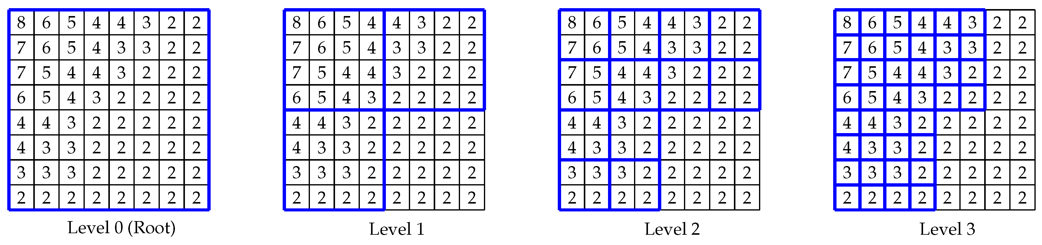
2.1. -Raster
2.2. Unary Codes and Notation
2.3. Elias Codes
2.4. Rice Codes
2.5. Simple9, Simple16, and PForDelta
2.6. Directly Addressable Codes
2.7. Selection of the k Value
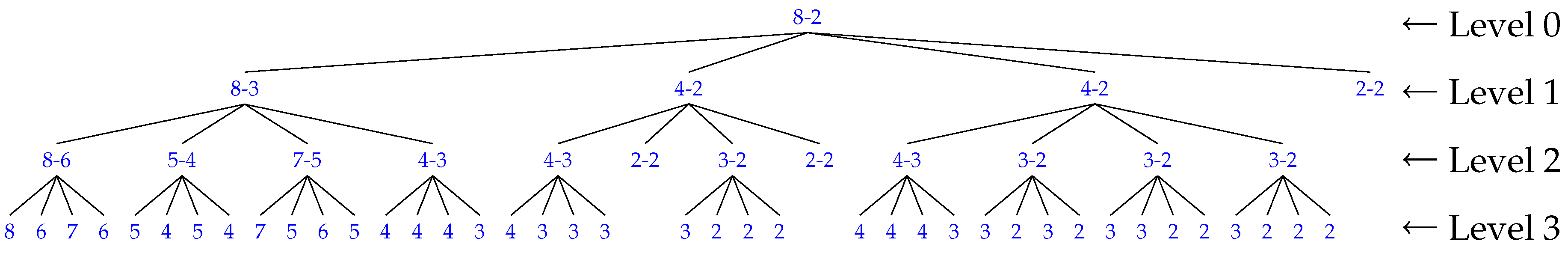
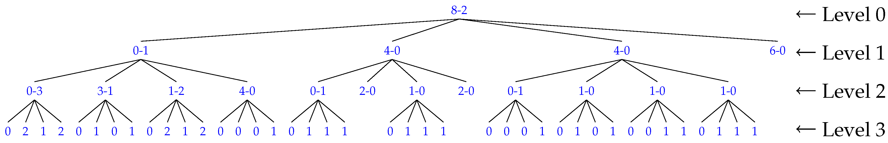
2.8. Heuristic -Raster
2.9. 3D-2D Mapping
3. Experimental Results
3.1. Best k Value Selection
3.2. Heuristic -Raster
3.3. 3D-2D Mapping
3.4. Comparison of Integer Encoders for -Raster
4. Conclusions
Author Contributions
Funding
Conflicts of Interest
References
- Clark, R.N.; Roush, T.L. Reflectance spectroscopy: Quantitative analysis techniques for remote sensing applications. J. Geophys. Res. Solid Earth 1984, 89, 6329–6340. [Google Scholar] [CrossRef]
- Goetz, A.F.; Vane, G.; Solomon, J.E.; Rock, B.N. Imaging spectrometry for earth remote sensing. Science 1985, 228, 1147–1153. [Google Scholar] [CrossRef] [PubMed]
- Kruse, F.A.; Lefkoff, A.; Boardman, J.; Heidebrecht, K.; Shapiro, A.; Barloon, P.; Goetz, A. The spectral image processing system (SIPS)-interactive visualization and analysis of imaging spectrometer data. AIP Conf. Proc. 1993, 283, 192–201. [Google Scholar]
- Joseph, W. Automated spectral analysis: A geologic example using AVIRIS data, north Grapevine Mountains, Nevada. In Proceedings of the Tenth Thematic Conference on Geologic Remote Sensing, Environmental Research Institute of Michigan, San Antonio, TX, USA, 9–12 May 1994; pp. 1407–1418. [Google Scholar]
- Asner, G.P. Biophysical and biochemical sources of variability in canopy reflectance. Remote Sens. Environ. 1998, 64, 234–253. [Google Scholar] [CrossRef]
- Parente, M.; Kerekes, J.; Heylen, R. A Special Issue on Hyperspectral Imaging [From the Guest Editors]. IEEE Geosci. Remote Sens. Mag. 2019, 7, 6–7. [Google Scholar] [CrossRef]
- Ientilucci, E.J.; Adler-Golden, S. Atmospheric Compensation of Hyperspectral Data: An Overview and Review of In-Scene and Physics-Based Approaches. IEEE Geosci. Remote Sens. Mag. 2019, 7, 31–50. [Google Scholar] [CrossRef]
- Khan, M.J.; Khan, H.S.; Yousaf, A.; Khurshid, K.; Abbas, A. Modern trends in hyperspectral image analysis: A review. IEEE Access 2018, 6, 14118–14129. [Google Scholar] [CrossRef]
- Theiler, J.; Ziemann, A.; Matteoli, S.; Diani, M. Spectral Variability of Remotely Sensed Target Materials: Causes, Models, and Strategies for Mitigation and Robust Exploitation. IEEE Geosci. Remote Sens. Mag. 2019, 7, 8–30. [Google Scholar] [CrossRef]
- Sun, W.; Du, Q. Hyperspectral band selection: A review. IEEE Geosci. Remote Sens. Mag. 2019, 7, 118–139. [Google Scholar] [CrossRef]
- Scafutto, R.D.M.; de Souza Filho, C.R.; de Oliveira, W.J. Hyperspectral remote sensing detection of petroleum hydrocarbons in mixtures with mineral substrates: Implications for onshore exploration and monitoring. ISPRS J. Photogramm. Remote Sens. 2017, 128, 146–157. [Google Scholar] [CrossRef]
- Bishop, C.A.; Liu, J.G.; Mason, P.J. Hyperspectral remote sensing for mineral exploration in Pulang, Yunnan Province, China. Int. J. Remote Sens. 2011, 32, 2409–2426. [Google Scholar] [CrossRef]
- Le Marshall, J.; Jung, J.; Zapotocny, T.; Derber, J.; Treadon, R.; Lord, S.; Goldberg, M.; Wolf, W. The application of AIRS radiances in numerical weather prediction. Aust. Meteorol. Mag. 2006, 55, 213–217. [Google Scholar]
- Robichaud, P.R.; Lewis, S.A.; Laes, D.Y.; Hudak, A.T.; Kokaly, R.F.; Zamudio, J.A. Postfire soil burn severity mapping with hyperspectral image unmixing. Remote Sens. Environ. 2007, 108, 467–480. [Google Scholar] [CrossRef] [Green Version]
- Navarro, G. Compact Data Structures: A Practical Approach; Cambridge University Press: Cambridge, UK, 2016. [Google Scholar]
- Jacobson, G. Space-efficient static trees and graphs. In Proceedings of the 30th Annual Symposium on Foundations of Computer Science, Research Triangle Park, NC, USA, 30 October–1 November 1989; pp. 549–554. [Google Scholar]
- Consultative Committee for Space Data Systems (CCSDS). Image Data Compression CCSDS 123.0-B-1; Blue Book; CCSDS: Washington, DC, USA, 2012. [Google Scholar]
- Jolliffe, I.T. Principal Component Analysis; Springer: Berlin, Germany, 2002; p. 487. [Google Scholar]
- Taubman, D.S.; Marcellin, M.W. JPEG 2000: Image Compression Fundamentals, Standards and Practice; Kluwer Academic Publishers: Boston, MA, USA, 2001. [Google Scholar]
- Chow, K.; Tzamarias, D.E.O.; Blanes, I.; Serra-Sagristà, J. Using Predictive and Differential Methods with K2-Raster Compact Data Structure for Hyperspectral Image Lossless Compression. Remote Sens. 2019, 11, 2461. [Google Scholar] [CrossRef] [Green Version]
- Elias, P. Efficient storage and retrieval by content and address of static files. J. ACM (JACM) 1974, 21, 246–260. [Google Scholar] [CrossRef]
- Ottaviano, G.; Venturini, R. Partitioned Elias-Fano indexes. In Proceedings of the 37th International ACM SIGIR Conference on Research & Development in Information Retrieval, Gold Coast, Australia, 6–11 July 2014; pp. 273–282. [Google Scholar]
- Pibiri, G.E. Dynamic Elias-Fano Encoding. Master’s Thesis, University of Pisa, Pisa, Italy, 2014. [Google Scholar]
- Sugiura, R.; Kamamoto, Y.; Harada, N.; Moriya, T. Optimal Golomb-Rice Code Extension for Lossless Coding of Low-Entropy Exponentially Distributed Sources. IEEE Trans. Inf. Theory 2018, 64, 3153–3161. [Google Scholar] [CrossRef]
- Rice, R.; Plaunt, J. Adaptive variable-length coding for efficient compression of spacecraft television data. IEEE Trans. Commun. Technol. 1971, 19, 889–897. [Google Scholar] [CrossRef]
- Rojals, J.S.; Karczewicz, M.; Joshi, R.L. Rice Parameter Update for Coefficient Level Coding in Video Coding Process. U.S. Patent 9,936,200, 3 April 2018. [Google Scholar]
- Zukowski, M.; Heman, S.; Nes, N.; Boncz, P. Super-scalar RAM-CPU cache compression. In Proceedings of the 22nd International Conference on Data Engineering (ICDE’06), Atlanta, GA, USA, 3–7 April 2006; p. 59. [Google Scholar]
- Silva-Coira, F. Compact Data Structures for Large and Complex Datasets. Ph.D. Thesis, Universidade da Coruña, A Coruña, Spain, 2017. [Google Scholar]
- Al Hasib, A.; Cebrian, J.M.; Natvig, L. V-PFORDelta: Data compression for energy efficient computation of time series. In Proceedings of the 2015 IEEE 22nd International Conference on High Performance Computing (HiPC), Bengaluru, India, 16–19 December 2015; pp. 416–425. [Google Scholar]
- Brisaboa, N.R.; Ladra, S.; Navarro, G. DACs: Bringing direct access to variable-length codes. Inf. Process. Manag. 2013, 49, 392–404. [Google Scholar] [CrossRef] [Green Version]
- Brisaboa, N.R.; Ladra, S.; Navarro, G. Directly addressable variable-length codes. In Proceedings of the International Symposium on String Processing and Information Retrieval, Saariselkä, Finland, 25–27 August 2009; pp. 122–130. [Google Scholar]
- Baruch, G.; Klein, S.T.; Shapira, D. A space efficient direct access data structure. J. Discret. Algorithms 2017, 43, 26–37. [Google Scholar] [CrossRef]
- Ladra, S.; Paramá, J.R.; Silva-Coira, F. Scalable and queryable compressed storage structure for raster data. Inf. Syst. 2017, 72, 179–204. [Google Scholar] [CrossRef]
- Cruces, N.; Seco, D.; Gutiérrez, G. A compact representation of raster time series. In Proceedings of the Data Compression Conference (DCC), Snowbird, UT, USA, 26–29 March 2019; pp. 103–111. [Google Scholar]
- Brisaboa, N.R.; Ladra, S.; Navarro, G. k 2-trees for compact web graph representation. In Proceedings of the International Symposium on String Processing and Information Retrieval, Saariselkä, Finland, 25–27 August 2009; pp. 18–30. [Google Scholar]
- Anh, V.N.; Moffat, A. Inverted index compression using word-aligned binary codes. Inf. Retr. 2005, 8, 151–166. [Google Scholar] [CrossRef]
- Zhang, J.; Long, X.; Suel, T. Performance of compressed inverted list caching in search engines. In Proceedings of the 17th International Conference on World Wide Web, Beijing, China, 21–25 April 2008; pp. 387–396. [Google Scholar]
- Gog, S.; Beller, T.; Moffat, A.; Petri, M. From theory to practice: Plug and play with succinct data structures. In Proceedings of the International Symposium on Experimental Algorithms, Copenhagen, Denmark, 29 June–1 July 2014; pp. 326–337. [Google Scholar]


| T Bitmap | binary | 1110 1111 1010 1111 | |
| decimal | Level 1 | 0446 | |
| Level 2 | 0314 0212 0111 | ||
| Level 3 | 0212 0101 0212 0001 0111 0111 0001 0101 0011 0111 | ||
| decimal | Level 1 | 100 | |
| Level 2 | 3120 10 1000 | ||
| decimal | 8 | ||
| decimal | 2 |
| Value | Rice Code | ||||
|---|---|---|---|---|---|
| Decimal | Binary | ||||
| Selector | Number of Integers | Width of Integers (Bits) | Wasted Bits |
|---|---|---|---|
| 0 | 28 | 1 | 0 |
| 1 | 14 | 2 | 0 |
| 2 | 9 | 3 | 1 |
| 3 | 7 | 4 | 0 |
| 4 | 5 | 5 | 3 |
| 5 | 4 | 7 | 0 |
| 6 | 3 | 9 | 1 |
| 7 | 2 | 14 | 0 |
| 8 | 1 | 28 | 0 |
| Selector | Number of Integers | Width of Integers (Bits) | |||
| 0 | 28 | ||||
| 1 | 21 | ||||
| 2 | 21 | ||||
| 3 | 21 | ||||
| 4 | 14 | ||||
| 5 | 9 | ||||
| 6 | 8 | ||||
| 7 | 7 | ||||
| 8 | 6 | ||||
| 9 | 6 | ||||
| 10 | 5 | ||||
| 11 | 5 | ||||
| 12 | 4 | ||||
| 13 | 3 | ||||
| 14 | 2 | ||||
| 15 | 1 | ||||
| Element | Selector | Number of Integers | Integers Stored (Decimal) | Integers Stored (Binary) |
|---|---|---|---|---|
| 0 | 7 (0111) | 2 | 3591 25 | 00111000000111 00000000011001 |
| 1 | 4 (0100) | 5 | 13 12 15 12 11 | 01101 01100 01111 01100 01011 |
| 2 | 4 (0100) | 5 | 26 20 8 13 8 | 11010 10100 01000 01101 01000 |
| 3 | 3 (0011) | 7 | 9 7 13 10 12 0 10 | 1001 0111 1101 1010 1100 0000 1010 |
| Decimal | Binary | DACs Blocks |
| 7 | 0111 | (BA) |
| 41 | 0101 1001 | (BA BA) |
| 100 | 0001 1100 1100 | (BA BA BA) |
| 63 | 0111 1111 | (BA BA) |
| 427 | 0110 1101 1011 | (BA BA BA) |
| Codeword | Frequency |
| 0111 | 3 |
| 0212 | 2 |
| 0101 | 2 |
| 0001 | 2 |
| 0011 | 1 |
| Sensor | Name | C/U | Acronym | Original Dimensions (x × y × z) | Bit Depth (bpppb) | Best k Value | -Raster Bit Rate (bpppb) | -Raster Bit-Rate Reduction (%) |
|---|---|---|---|---|---|---|---|---|
| AIRS | 9 | U | AG9 | 90 × 135 × 1501 | 12 | 6 | 9.49 | 21% |
| 16 | U | AG16 | 90 × 135 × 1501 | 12 | 6 | 9.12 | 24% | |
| 60 | U | AG60 | 90 × 135 × 1501 | 12 | 15 | 9.72 | 19% | |
| 126 | U | AG126 | 90 × 135 × 1501 | 12 | 6 | 9.61 | 20% | |
| 129 | U | AG129 | 90 × 135 × 1501 | 12 | 6 | 8.65 | 28% | |
| 151 | U | AG151 | 90 × 135 × 1501 | 12 | 6 | 9.53 | 21% | |
| 182 | U | AG182 | 90 × 135 × 1501 | 12 | 6 | 9.68 | 19% | |
| 193 | U | AG193 | 90 × 135 × 1501 | 12 | 15 | 9.30 | 23% | |
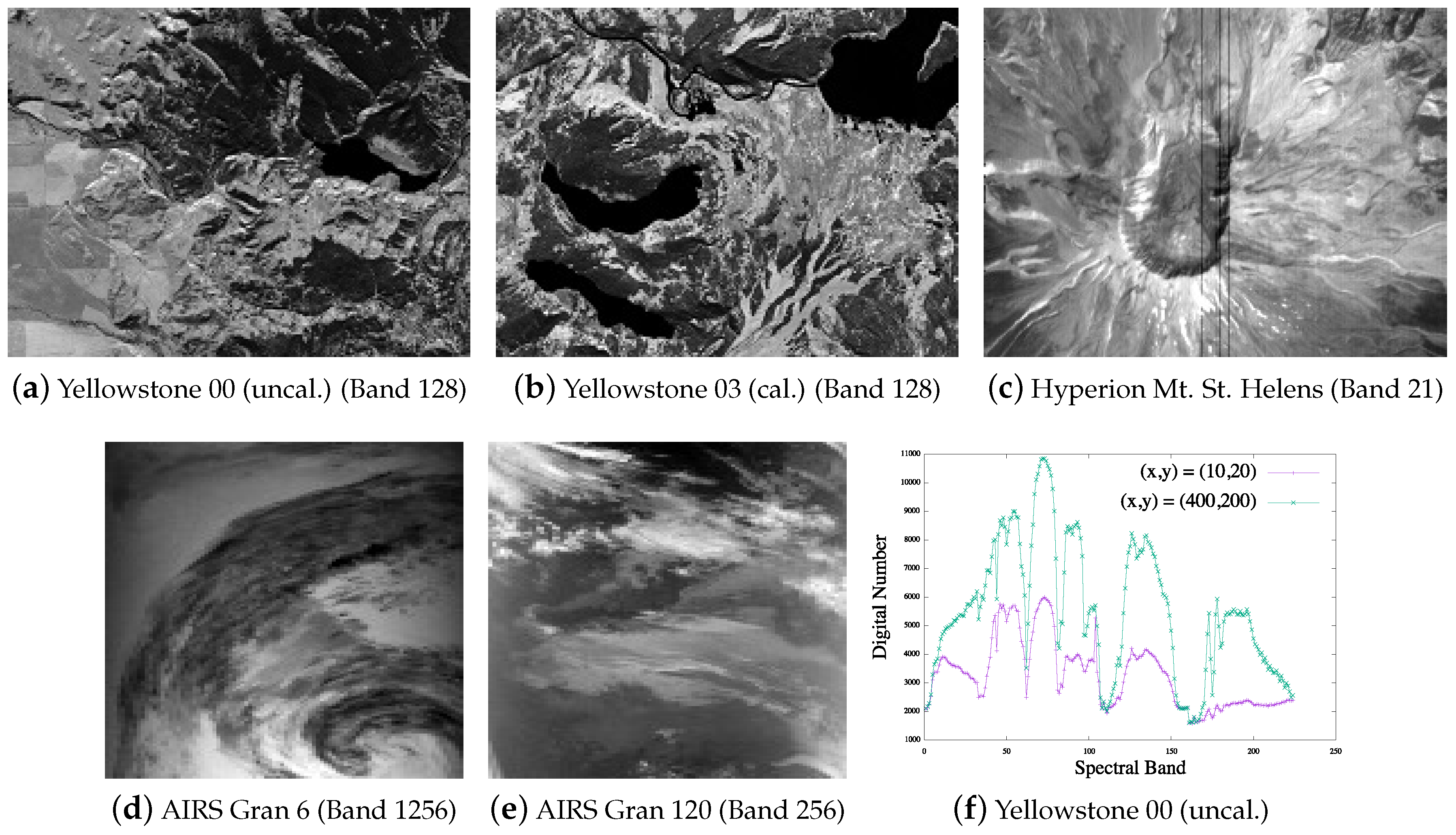
| AVIRIS | Yellowstone sc. 00 | C | ACY00 | 677 × 512 × 224 | 16 | 6 | 9.61 | 40% |
| Yellowstone sc. 03 | C | ACY03 | 677 × 512 × 224 | 16 | 6 | 9.42 | 41% | |
| Yellowstone sc. 10 | C | ACY10 | 677 × 512 × 224 | 16 | 6 | 7.62 | 52% | |
| Yellowstone sc. 11 | C | ACY11 | 677 × 512 × 224 | 16 | 6 | 8.81 | 45% | |
| Yellowstone sc. 18 | C | ACY18 | 677 × 512 × 224 | 16 | 6 | 9.78 | 39% | |
| Yellowstone sc. 00 | U | AUY00 | 680 × 512 × 224 | 16 | 9 | 11.92 | 25% | |
| Yellowstone sc. 03 | U | AUY03 | 680 × 512 × 224 | 16 | 9 | 11.74 | 27% | |
| Yellowstone sc. 10 | U | AUY10 | 680 × 512 × 224 | 16 | 9 | 9.99 | 38% | |
| Yellowstone sc. 11 | U | AUY11 | 680 × 512 × 224 | 16 | 9 | 11.27 | 30% | |
| Yellowstone sc. 18 | U | AUY18 | 680 × 512 × 224 | 16 | 9 | 12.15 | 24% | |
| CRISM | frt000065e6_07_sc164 | U | C164 | 640 × 420 × 545 | 12 | 6 | 10.08 | 16% |
| frt00008849_07_sc165 | U | C165 | 640 × 450 × 545 | 12 | 6 | 10.37 | 14% | |
| frt0001077d_07_sc166 | U | C166 | 640 × 480 × 545 | 12 | 6 | 11.05 | 8% | |
| hrl00004f38_07_sc181 | U | C181 | 320 × 420 × 545 | 12 | 5 | 9.97 | 17% | |
| hrl0000648f_07_sc182 | U | C182 | 320 × 450 × 545 | 12 | 5 | 10.11 | 16% | |
| hrl0000ba9c_07_sc183 | U | C183 | 320 × 480 × 545 | 12 | 5 | 10.65 | 11% | |
| Hyperion | Agricultural | C | HCA | 256 × 3129 × 242 | 12 | 16 | 8.52 | 29% |
| Coral Reef | C | HCC | 256 × 3127 × 242 | 12 | 8 | 7.62 | 36% | |
| Urban | C | HCU | 256 × 2905 × 242 | 12 | 16 | 8.85 | 26% | |
| Erta Ale | U | HUEA | 256 × 3187 × 242 | 12 | 8 | 7.76 | 35% | |
| Lake Monona | U | HULM | 256 × 3176 × 242 | 12 | 8 | 7.82 | 35% | |
| Mt. St. Helena | U | HUMS | 256 × 3242 × 242 | 12 | 8 | 7.91 | 34% | |
| IASI | Level 0 1 | U | I01 | 60 × 1528 × 8359 | 12 | 12 | 6.32 | 47% |
| Level 0 2 | U | I02 | 60 × 1528 × 8359 | 12 | 12 | 6.38 | 47% | |
| Level 0 3 | U | I03 | 60 × 1528 × 8359 | 12 | 12 | 6.31 | 47% | |
| Level 0 4 | U | I04 | 60 × 1528 × 8359 | 12 | 12 | 6.43 | 46% |
| Scene Data (w × h) | = 2 | 3 | 4 | 5 | 6 | 7 | 8 | 9 | 10 | 11 | 12 | 13 | 14 | 15 | 16 | 17 | 18 | 19 | 20 | |
|---|---|---|---|---|---|---|---|---|---|---|---|---|---|---|---|---|---|---|---|---|
| AG9 (90 × 135) | S | 256 | 243 | 256 | 625 | 216 | 343 | 512 | 729 | 1000 | 1331 | 144 | 169 | 196 | 225 | 256 | 289 | 324 | 361 | 400 |
| C | 13.06 | 10.11 | 10.03 | 10.47 | 9.49 | 9.98 | 10.68 | 9.89 | 10.65 | 12.98 | 11.23 | 10.33 | 11.29 | 9.53 | 11.57 | 11.72 | 10.78 | 12.52 | 12.13 | |
| B | 5.3 | 3.2 | 4.1 | 10.9 | 4.2 | 10.9 | 12.6 | 10.7 | 17.5 | 29.6 | 2.9 | 4.1 | 3.0 | 4.3 | 4.6 | 6.6 | 6.8 | 4.9 | 7.3 | |
| ACY00 (677 × 512) | S | 1024 | 729 | 1024 | 3125 | 1296 | 2401 | 4096 | 729 | 1000 | 1331 | 1728 | 2197 | 2744 | 3375 | 4096 | 4913 | 5832 | 6859 | 8000 |
| C | 12.34 | 10.20 | 9.76 | 10.70 | 9.61 | 9.91 | 10.26 | 9.69 | 9.83 | 9.87 | 9.95 | 10.24 | 10.20 | 10.51 | 10.24 | 10.55 | 10.61 | 10.49 | 10.73 | |
| B | 19.5 | 10.7 | 10.8 | 30.7 | 10.5 | 19.3 | 42.0 | 8.8 | 9.3 | 11.5 | 13.2 | 17.1 | 23.2 | 29.1 | 45.5 | 55.8 | 72.6 | 101.1 | 131.0 | |
| AUY00 (680 × 512) | S | 1024 | 729 | 1024 | 3125 | 1296 | 2401 | 4096 | 729 | 1000 | 1331 | 1728 | 2197 | 2744 | 3375 | 4096 | 4913 | 5832 | 6859 | 8000 |
| C | 15.31 | 12.93 | 12.20 | 13.06 | 12.08 | 12.35 | 12.47 | 11.92 | 12.11 | 12.13 | 12.17 | 12.52 | 12.43 | 12.84 | 12.44 | 12.83 | 12.87 | 12.69 | 12.96 | |
| B | 18.4 | 10.7 | 10.1 | 30.7 | 11.4 | 20.9 | 41.4 | 7.7 | 8.5 | 10.9 | 12.7 | 17.1 | 22.9 | 29.3 | 44.3 | 55.8 | 73.0 | 101.0 | 130.6 | |
| C164 (640 × 420) | S | 1024 | 729 | 1024 | 3125 | 1296 | 2401 | 4096 | 729 | 1000 | 1331 | 1728 | 2197 | 2744 | 3375 | 4096 | 4913 | 5832 | 6859 | 8000 |
| C | 12.60 | 10.42 | 10.17 | 11.35 | 10.08 | 10.46 | 11.12 | 10.34 | 10.20 | 10.76 | 10.48 | 10.96 | 10.66 | 10.77 | 11.19 | 11.18 | 11.55 | 11.80 | 11.30 | |
| B | 47.1 | 28.8 | 27.9 | 74.3 | 27.7 | 47.3 | 98.6 | 19.3 | 21.1 | 24.8 | 29.7 | 38.7 | 49.4 | 69.6 | 96.2 | 133.3 | 179.3 | 231.1 | 314.9 | |
| HCA (256 × 3129) | S | 4096 | 6561 | 4096 | 15625 | 7776 | 16807 | 4096 | 6561 | 10000 | 14641 | 20736 | 28561 | 38416 | 3375 | 4096 | 4913 | 5832 | 6859 | 8000 |
| C | 17.2 | 15.64 | 9.79 | - | 10.47 | - | 8.54 | 9.13 | 9.7 | - | - | - | - | 8.65 | 8.52 | 8.75 | 9.16 | 9.07 | 8.92 | |
| B | 121.9 | 183.6 | 68.7 | - | 186.6 | - | 55.2 | 115.6 | 238.9 | - | - | - | - | 44.3 | 56.7 | 70.6 | 91.9 | 121.8 | 156.6 | |
| HUEA (256 × 3187) | S | 4096 | 6561 | 4096 | 15625 | 7776 | 16807 | 4096 | 6561 | 10000 | 14641 | 20736 | 28561 | 38416 | 3375 | 4096 | 4913 | 5832 | 6859 | 8000 |
| C | 16.02 | 14.63 | 8.89 | - | 9.68 | - | 7.76 | 8.46 | 9.00 | - | - | - | - | 8.50 | 7.80 | 8.69 | 8.68 | 8.46 | 8.27 | |
| B | 131.1 | 189.0 | 74.4 | - | 172.3 | - | 60.3 | 120.8 | 245.3 | - | - | - | - | 49.5 | 60.4 | 75.7 | 95.3 | 123.3 | 159.4 | |
| I01 (60 × 1528) | S | 2048 | 2187 | 4096 | 3125 | 7776 | 2401 | 4096 | 6561 | 10000 | 14641 | 1728 | 2197 | 2744 | 3375 | 4096 | 4913 | 5832 | 6859 | 8000 |
| C | 21.99 | 12.59 | 17.98 | 10.25 | 24.60 | 7.71 | 9.33 | 12.23 | 16.97 | 26.49 | 6.32 | 7.28 | 8.28 | 6.80 | 7.64 | 8.54 | 9.44 | 10.43 | 8.25 | |
| B | 1021.1 | 780.5 | 1728.7 | 986.5 | 5167.5 | 635.6 | 1426.7 | 3938.6 | 7870.7 | 17973.9 | 339.7 | 474.3 | 658.9 | 944.0 | 1498.1 | 1826.6 | 2789.8 | 3543.2 | 4810.3 |
| Scene Data (w × h) | = 2 | 3 | 4 | 5 | 6 | 7 | 8 | 9 | 10 | 11 | 12 | 13 | 14 | 15 | 16 | 17 | 18 | 19 | 20 |
|---|---|---|---|---|---|---|---|---|---|---|---|---|---|---|---|---|---|---|---|
| AG9 (90 × 135) | 2.45 | 1.20 | 0.91 | 0.82 | 0.70 | 0.65 | 0.61 | 0.64 | 0.61 | 0.57 | 0.47 | 0.47 | 0.48 | 0.47 | 0.45 | 0.42 | 0.46 | 0.43 | 0.43 |
| ACY00 (677 × 512) | 15.10 | 4.95 | 2.89 | 2.07 | 1.60 | 1.33 | 1.13 | 1.01 | 0.89 | 0.88 | 0.79 | 0.76 | 0.74 | 0.73 | 0.69 | 0.67 | 0.68 | 0.66 | 0.64 |
| AUY00 (680 × 512) | 17.07 | 5.70 | 3.03 | 2.19 | 1.66 | 1.40 | 1.20 | 1.05 | 0.94 | 0.88 | 0.85 | 0.83 | 0.80 | 0.77 | 0.72 | 0.77 | 0.72 | 0.70 | 0.72 |
| C164 (640 × 420) | 14.66 | 5.09 | 2.84 | 2.12 | 1.67 | 1.48 | 1.34 | 1.10 | 1.08 | 1.01 | 0.95 | 0.93 | 0.88 | 0.83 | 0.81 | 0.81 | 0.79 | 0.74 | 0.74 |
| HCA (256 × 3129) | 0.34 | 0.26 | 0.19 | - | 0.19 | - | 0.18 | 0.18 | 0.16 | - | - | - | - | 0.17 | 0.14 | 0.15 | 0.15 | 0.16 | 0.16 |
| HUEA (256 × 3187) | 31.59 | 10.09 | 5.24 | - | 3.11 | - | 1.87 | 1.81 | 1.60 | - | - | - | - | 1.22 | 1.02 | 1.01 | 1.01 | 1.00 | 1.01 |
| I01 (60 × 1528) | 6.13 | 3.35 | 2.48 | 2.24 | 2.13 | 1.94 | 1.82 | 1.76 | 1.74 | 1.72 | 1.62 | 1.56 | 1.48 | 1.55 | 1.54 | 1.54 | 1.41 | 1.40 | 1.53 |
| AIRS Granule | -Raster () (Best) | -Raster () (Optimal) | -Raster () | -Raster () |
| AG9 | 9.49 | 9.53 | 13.06 | 13.22 |
| AG16 | 9.12 | 9.17 | 12.72 | 12.85 |
| AG60 | 9.81 | 9.72 | 13.65 | 13.86 |
| AG126 | 9.61 | 9.72 | 13.42 | 13.59 |
| AG129 | 8.65 | 8.72 | 11.98 | 11.95 |
| AG151 | 9.53 | 9.56 | 13.19 | 13.35 |
| AG182 | 9.68 | 9.71 | 13.32 | 13.47 |
| AG193 | 9.44 | 9.30 | 13.29 | 13.43 |
| AVIRIS Uncalibrated | -Raster () (Best) | -Raster () (Optimal) | -Raster () | -Raster () |
| AUY00 | 11.92 | 11.92 | 15.31 | 15.19 |
| AUY03 | 11.74 | 11.74 | 15.03 | 14.74 |
| AUY10 | 9.99 | 9.99 | 12.85 | 11.86 |
| AUY11 | 11.27 | 11.27 | 14.27 | 14.08 |
| AUY18 | 12.15 | 12.15 | 15.36 | 15.25 |
| Band | Original Size | -Tree | -Tree | -Tree |
|---|---|---|---|---|
| All bands | 16 | 16.53 | 20.57 | 26.57 |
| 1481 | 16 | 17.56 | 22.00 | 28.45 |
| 1482 | 16 | 17.27 | 21.54 | 27.84 |
| 1483 | 16 | 17.19 | 21.47 | 27.67 |
| 1484 | 16 | 17.45 | 21.81 | 28.18 |
| 1485 | 16 | 16.93 | 21.10 | 27.29 |
| 1486 | 16 | 17.09 | 21.27 | 27.50 |
| 1487 | 16 | 16.82 | 21.06 | 27.02 |
| 1488 | 16 | 17.01 | 21.21 | 27.34 |
| 1489 | 16 | 17.23 | 21.51 | 27.78 |
| 1490 | 16 | 16.94 | 21.10 | 27.20 |
| 1491 | 16 | 16.80 | 20.86 | 26.96 |
| 1492 | 16 | 16.56 | 20.64 | 26.51 |
| 1493 | 16 | 16.80 | 20.91 | 26.89 |
| 1494 | 16 | 16.84 | 20.93 | 26.98 |
| 1495 | 16 | 16.69 | 20.88 | 26.72 |
| 1496 | 16 | 16.66 | 20.75 | 26.66 |
| 1497 | 16 | 16.70 | 20.87 | 26.73 |
| 1498 | 16 | 16.61 | 20.70 | 26.58 |
| 1499 | 16 | 16.67 | 20.73 | 26.78 |
| 1500 | 16 | 16.39 | 20.40 | 26.18 |
| Hyperspectral Scene | Entropy () | Rice ( Value) | Simple9 | PForDelta | Simple16 | DACs (Best ) | DACs (Optimal ) | gzip |
|---|---|---|---|---|---|---|---|---|
| AG9 | 8.29 | 10.10 (7) | 10.06 | 9.88 | 9.69 | 9.49 (6) | 9.53 (15) | 12.45 |
| AG16 | 7.92 | 9.88 (7) | 9.64 | 9.55 | 9.30 | 9.12 (6) | 9.17 (15) | 11.96 |
| AG60 | 8.58 | 10.31 (7) | 10.50 | 10.19 | 10.12 | 9.72 (15) | 9.81 (6) | 12.79 |
| AG126 | 8.42 | 10.34 (7) | 10.25 | 9.98 | 9.81 | 9.61 (6) | 9.72 (15) | 12.55 |
| AG129 | 7.47 | 9.66 (7) | 9.01 | 9.01 | 8.61 | 8.65 (6) | 8.72 (15) | 11.21 |
| AG151 | 8.36 | 10.39 (7) | 9.99 | 9.79 | 9.54 | 9.53 (6) | 9.56 (15) | 12.39 |
| AG182 | 8.44 | 10.58 (7) | 10.44 | 10.09 | 10.01 | 9.68 (6) | 9.71 (15) | 12.71 |
| AG193 | 8.25 | 10.26 (7) | 10.06 | 9.93 | 9.65 | 9.30 (15) | 9.44 (6) | 12.33 |
| ACY00 | 8.81 | 9.89 (7) | 10.37 | 9.80 | 10.11 | 9.61 (6) | 9.69 (9) | 12.56 |
| ACY03 | 8.48 | 9.70 (7) | 9.80 | 9.40 | 9.57 | 9.42 (6) | 9.50 (9) | 11.98 |
| ACY10 | 6.88 | 9.18 (7) | 7.34 | 7.43 | 7.18 | 7.62 (6) | 7.74 (9) | 9.32 |
| ACY11 | 8.12 | 9.45 (7) | 9.32 | 9.02 | 9.09 | 8.81 (6) | 9.00 (9) | 11.61 |
| ACY18 | 8.96 | 10.58 (7) | 10.52 | 9.84 | 10.28 | 9.78 (6) | 9.88 (9) | 12.66 |
| AUY00 | 11.16 | 17.59 (7) | 14.01 | 11.93 | 13.79 | 11.92 (9) | 11.92 (9) | 15.13 |
| AUY03 | 10.83 | 16.59 (7) | 13.54 | 11.56 | 13.29 | 11.74 (9) | 11.74 (9) | 14.59 |
| AUY10 | 9.26 | 12.87 (7) | 10.90 | 9.61 | 10.54 | 9.99 (9) | 9.99 (9) | 12.29 |
| AUY11 | 10.60 | 15.16 (7) | 13.12 | 11.24 | 12.89 | 11.27 (9) | 11.27 (9) | 14.47 |
| AUY18 | 11.38 | 20.70 (7) | 14.19 | 12.10 | 14.01 | 12.15 (9) | 12.15 (9) | 15.53 |
| C164 | 9.18 | 10.33 (7) | 11.35 | 10.44 | 11.14 | 10.08 (6) | 10.08 (6) | 12.85 |
| C165 | 9.48 | 10.91 (7) | 11.78 | 10.69 | 11.57 | 10.37 (6) | 10.37 (6) | 13.17 |
| C166 | 10.02 | 12.83 (7) | 12.99 | 11.41 | 12.74 | 11.05 (6) | 11.05 (6) | 13.61 |
| C181 | 9.16 | 9.96 (7) | 10.93 | 10.53 | 10.72 | 9.97 (5) | 9.97 (5) | 13.37 |
| C182 | 9.27 | 10.17 (7) | 11.24 | 10.67 | 10.99 | 10.11 (5) | 10.11 (5) | 13.26 |
| C183 | 9.60 | 11.15 (7) | 12.33 | 11.21 | 12.05 | 10.65 (5) | 10.65 (5) | 13.32 |
| HCA | 7.59 | 8.94 (7) | 9.79 | 8.80 | 9.56 | 8.52 (16) | 8.54 (8) | 11.20 |
| HCC | 6.75 | 8.20 (7) | 8.28 | 7.60 | 7.93 | 7.62 (8) | 7.71 (16) | 9.51 |
| HCU | 7.87 | 9.78 (7) | 10.30 | 8.91 | 10.04 | 8.85 (16) | 8.86 (8) | 11.35 |
| HUEA | 6.66 | 7.67 (5) | 8.30 | 7.99 | 8.00 | 7.76 (8) | 7.80 (16) | 9.85 |
| HULM | 6.71 | 7.66 (5) | 8.38 | 8.11 | 8.10 | 7.82 (8) | 7.88 (16) | 10.13 |
| HUMS | 6.77 | 7.90 (5) | 8.48 | 8.14 | 8.20 | 7.91 (8) | 7.94 (16) | 10.12 |
| I01 | 5.39 | 6.51 (4) | 6.26 | 6.54 | 5.94 | 6.32 (12) | 6.80 (15) | 7.46 |
| I02 | 5.46 | 6.56 (4) | 6.27 | 6.55 | 5.96 | 6.38 (12) | 6.84 (15) | 7.51 |
| I03 | 5.42 | 6.51 (4) | 6.19 | 6.48 | 5.89 | 6.31 (12) | 6.79 (15) | 7.39 |
| I04 | 5.51 | 6.62 (4) | 6.37 | 6.65 | 6.04 | 6.43 (12) | 6.90 (15) | 7.63 |
© 2020 by the authors. Licensee MDPI, Basel, Switzerland. This article is an open access article distributed under the terms and conditions of the Creative Commons Attribution (CC BY) license (http://creativecommons.org/licenses/by/4.0/).
Share and Cite
Chow, K.; Tzamarias, D.E.O.; Hernández-Cabronero, M.; Blanes, I.; Serra-Sagristà, J. Analysis of Variable-Length Codes for Integer Encoding in Hyperspectral Data Compression with the k2-Raster Compact Data Structure. Remote Sens. 2020, 12, 1983. https://doi.org/10.3390/rs12121983
Chow K, Tzamarias DEO, Hernández-Cabronero M, Blanes I, Serra-Sagristà J. Analysis of Variable-Length Codes for Integer Encoding in Hyperspectral Data Compression with the k2-Raster Compact Data Structure. Remote Sensing. 2020; 12(12):1983. https://doi.org/10.3390/rs12121983
Chicago/Turabian StyleChow, Kevin, Dion Eustathios Olivier Tzamarias, Miguel Hernández-Cabronero, Ian Blanes, and Joan Serra-Sagristà. 2020. "Analysis of Variable-Length Codes for Integer Encoding in Hyperspectral Data Compression with the k2-Raster Compact Data Structure" Remote Sensing 12, no. 12: 1983. https://doi.org/10.3390/rs12121983