Comparative Assessment of Machine Learning Methods for Urban Vegetation Mapping Using Multitemporal Sentinel-1 Imagery


1
Chair of Photogrammetry and Remote Sensing, Faculty of Geodesy, University of Zagreb, 10000 Zagreb, Croatia
2
Chair of Geoinformatics, Faculty of Geodesy, University of Zagreb, 10000 Zagreb, Croatia
*
Author to whom correspondence should be addressed.
Remote Sens. 2020, 12(12), 1952; https://doi.org/10.3390/rs12121952
Submission received: 7 May 2020
/
Revised: 10 June 2020
/
Accepted: 15 June 2020
/
Published: 17 June 2020
(This article belongs to the Special Issue SAR for Forest Mapping)
Abstract
:Mapping of green vegetation in urban areas using remote sensing techniques can be used as a tool for integrated spatial planning to deal with urban challenges. In this context, multitemporal (MT) synthetic aperture radar (SAR) data have not been equally investigated, as compared to optical satellite data. This research compared various machine learning methods using single-date and MT Sentinel-1 (S1) imagery. The research was focused on vegetation mapping in urban areas across Europe. Urban vegetation was classified using six classifiers—random forests (RF), support vector machine (SVM), extreme gradient boosting (XGB), multi-layer perceptron (MLP), AdaBoost.M1 (AB), and extreme learning machine (ELM). Whereas, SVM showed the best performance in the single-date image analysis, the MLP classifier yielded the highest overall accuracy in the MT classification scenario. Mean overall accuracy (OA) values for all machine learning methods increased from 57% to 77% with speckle filtering. Using MT SAR data, i.e., three and five S1 imagery, an additional increase in the OA of 8.59% and 13.66% occurred, respectively. Additionally, using three and five S1 imagery for classification, the F1 measure for forest and low vegetation land-cover class exceeded 90%. This research allowed us to confirm the possibility of MT C-band SAR imagery for urban vegetation mapping.

1. Introduction
Remote sensing could provide reliable land-cover classification maps, through the active microwave and passive optical sensors, which could be used for a wide range of applications. The monitoring of urban vegetation at a regional scale has become an important topic, since urban development leads to a slow but steady degradation of urban green vegetation [1].
Urban areas are complex systems composed of numerous interacting components that evolve over multiple spatio-temporal scales [2]. In this context, a multispectral optical image is easy for interpretation and classification, but often climate conditions limit the utilization of this satellite imagery [3]. Conversely, synthetic aperture radar (SAR) systems are independent of weather and sun illumination and provide the all-weather mapping capability [4]. However, due to the coherent mode of backscattered signal processing [5], speckle noise cannot be avoided and will be present in SAR images [6]. The speckle noise degrades the quality of acquired imagery, causing difficulties for both manual and automatic image interpretation [7]. Therefore, speckle filtering is required for classification tasks, especially for detecting vegetation in urban systems whose components differ at various scales (urban forest, green roofs, urban gardens, parks). Many speckle filters have been implemented for the reduction of speckle noise in SAR imagery [8,9,10,11,12]. Spatial filters reduce the noise by using smoothing windows based on a weighted summation of neighboring pixels.
However, the spatial resolution on resulting SAR imagery deteriorates, and fine details fade away, which causes information loss [13]. Hence, urban vegetation mapping using single-date imagery often does not produce satisfactory results, and the use of the multitemporal (MT) SAR imagery are adequate for better differentiation of various land-cover classes, especially for vegetation [14,15,16,17,18]. With the launch of the Sentinel-1 (S1) SAR satellites, a large collection of MT S1 imagery of Central Europe with a temporal resolution of three days is available for different classification tasks. Veloso et al. [19] investigated the temporal behavior of the MT S1 imagery for agricultural applications. The dense time series of optical and SAR imagery allows them to capture phenological stages and to discriminate various crops. S1 backscatters, vertical–vertical (VV), and vertical–horizontal (VH) are more sensitive to surface scattering and volume scattering, respectively. In SAR imagery, urban areas are characterized by very bright reflections, since human-made objects behave as corner reflectors [1], while the predominant mechanism responsible for backscatter from vegetation is volume scattering, whose interpretation is a bit more complex [20]. Using S1 MT imagery at the field scale, Gao et al. [21] proposed a methodology for irrigation mapping. Analysis of MT SAR imagery enables us to define irrigated fields since single-date image analysis is not always reliable. The research is based on MT SAR data and can be applied for various classification tasks.
With the launch of satellite missions that enable systematic acquisitions within short revisit times (e.g., Sentinel-1), the MT series of SAR imagery are mostly used for flood and wetland monitoring [22,23,24], as floods are often associated with heavy rain that makes optical satellite data unavailable. Furthermore, SAR backscatter intensity values increase significantly during flood events due to the interaction between water and vegetation (e.g., trunks, stems), which enables the mapping of flooded vegetation [25]. SAR systems offer a possibility of acquiring data in a continuous manner, regardless of the weather and lighting conditions, which enables rapid mapping of environmental changes. However, compared to the optical satellite data, there are several challenges regarding SAR image analysis for land-cover applications (e.g., speckle, radar shadow caused by layover, and foreshortening). Additionally, due to the complex pre-processing and interpretation of radar data [25,26], numerous researchers still use optical satellite data for land-cover (LC) mapping (see Figure 1).
The MT series of SAR imagery are also used for mapping urban areas [27,28,29]. For urban vegetation mapping, MT SAR data have not been equally investigated, as compared to the optical satellite data [30,31,32]. Since Figure 1 shows that SAR imagery is neglected for LC classification tasks, in comparison to optical satellite data, this research evaluated the practical application of SAR data for LC classification. Therefore, the performance of the most used non-parametric machine learning methods for MT SAR imagery was assessed for urban vegetation mapping. In this research, the tested classifiers were random forests (RF), support vector machine (SVM), extreme gradient boosting (XGB), artificial neural network (ANN), AdaBoost.M1 (AB), and extreme learning machine (ELM). For the MT SAR imagery, RF and SVM were applied successfully for land-cover classification [18,33,34]. ANNs were used successfully for the land-cover mapping, and the classification accuracy was often significantly improved, compared to the aforementioned methods. In this research, a specific type of ANN—Multi-Layer Perceptron (MLP), as an ensemble of feedforward neural networks, was used. Over the past years, more and more research used MLP for the processing of SAR imagery [35,36,37]. Gradient boosting classifiers combine many “weak” learning models into a single composite classifier. XGB, developed by Chen and Guestrin [38], was investigated due to its novelty and lack of SAR land-cover and MT applications. AdaBoost [39] has already been proven in the remote sensing, e.g., LC classification of multispectral imagery [40,41] and hyperspectral remote sensing imagery [42,43]. In comparison to the backpropagation in the ANNs, ELM is a single layer feedforward neural network. Huang et al. [44] proposed the ELM classifier, which randomly chooses hidden nodes and bias, whereas [45] explored the potential of the ELM for LC classification.
Camargo et al. [46] and Lapini et al. [47] evaluated various classifiers using SAR imagery for LC classification of the Brazilian tropical savanna and forest classification in Mediterranean areas, respectively. Recent research presented RF, MLP, SVM, as the most accurate classifiers, and the DT J48 (DT—decision tree) classifier showed satisfactory performance for the detection of specific LC classes (e.g., vegetation). In contrast, in the latter study, RF achieved the best overall accuracy (OA), whereas SVM yielded a lower classification results due to the imbalanced number of samples among the classes. Waske and Braun [48] applied various classifier ensembles to MT C-band data for LC mapping. Classification accuracy of 84% was achieved in rural areas using RF classifier, which proved to be very well suited for LC classifications using MT stacks of SAR imagery.
The objective of this study was the mapping of vegetation in urban areas using MT C-band SAR imagery. Furthermore, this paper evaluated six different machine learning methods for classifying LC classes in three different study areas. The purpose of this research was to assess the possibility of vegetation mapping using MT S1 imagery in urban areas across Europe and on a related comparative assessment of different classifiers. The rest of the paper is organized as follows—(1) information about the study areas and SAR data used in this research; (2) description of pre-processing steps for S1 imagery and the tested classifiers for urban vegetation mapping; (3) results; (4) discussion, and (5) conclusions.
2. Study Areas and Dataset
2.1. Study Areas
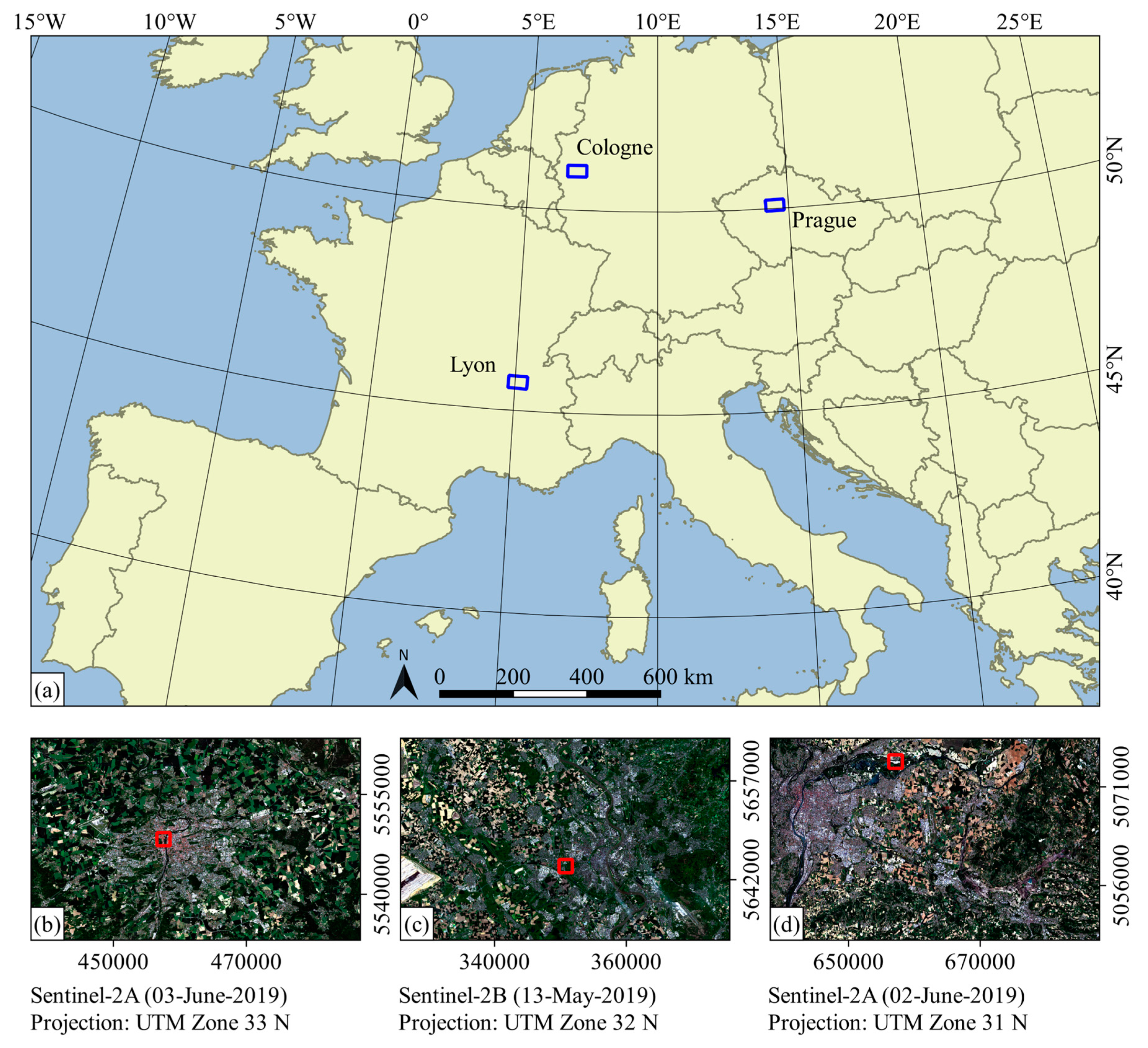
The study areas used in this research are shown in Figure 2. The first study area was Prague in the Czech Republic. The central part of the scene consisted of the urban area divided by the river Vltava. Most of the area in the south was agricultural land, either different types of crops or bare land, whereas the northern part of the scene was covered with forest, which separated the city from its outskirts. The second selected study area was Cologne, Germany. The western part was characterized by mainly flat terrain with agricultural fields and bare land areas, whereas eastern parts were dominated by forest areas. The central part of the scene was dominated by an urban area, with a lot of urban parks, lakes, and grasslands. Third, the considered study area was situated in Lyon, France. The city center with its surroundings was located in the western part of the scene, whereas other parts of the scene were dominated by vegetation and bare lands. Each study area had the same dimensions of approximately 30 km × 50 km, and the aforementioned areas were chosen because of a highly diverse landscape (more details about study areas are shown in Appendix A).
2.2. Data
The available S1 ground range detected (GRD) imagery with VV (vertical–vertical) and VH (vertical–horizontal) polarisations were acquired on the Sentinel Data Hub. For each study area, to ensure that the pixels remained unchanged in the same position over time, a reference date was chosen (i.e., 06 June 2019, 13 May 2019, and 04 June 2019 for Prague, Cologne, and Lyon, respectively). Since the constellation of Sentinel-1A (S1A) and Sentinel-1B (S1B) pass over the same spot on the ground every six days with identical orbit configuration (same image geometry), two scenes before and two scenes after the reference date (Table 1) in the same acquisition orbits were chosen for MT land-cover analysis (three scenes—MT_3; five scenes—MT_5).
3. Methods
3.1. Pre-Processing
To perform MT land-cover analysis using SAR imagery, several pre-processing steps are required. Pre-processing steps were executed with the Graph Processing Tools (GPT) of ESA’s Toolbox (S1TBX). It included radiometric calibration, terrain correction, and co-registration.
For the quantitative usage of the S1 Level-1 imagery, a radiometric calibration needed to be applied. The result of the calibration was values that represented the radar backscatter of the reflecting surface. The calibration reversed the scaling factor applied during product generation and applied a constant offset and a range-dependent gain, including the absolute calibration offset. In this research, raw signals from the GRD products were calibrated to the sigma naught (σ0) backscatter intensities.
GRD scenes have to be geocoded from a slant-range to a ground-range geometry, since the side-look view geometry of the SAR system, and Earth topography cause various distortions. Orthorectification of the S1 imagery (i.e., range doppler terrain correction operator) was conducted in the SNAP software, and the SAR scenes were terrain-corrected using the shuttle radar topography mission (SRTM) one-arcsecond tiles and were transformed to a universal transverse mercator (UTM) projection. The scenes were registered to a UTM Zone 33 N (Prague), Zone 32 N (Cologne), and Zone 31 N (Lyon), whereas WGS 1984 was used as an earth model.
In order to conduct LC classification in a time-series, image co-registration was needed to ensure that the images were spatially aligned. A set of images had to be aligned on a pixel scale, since wrong co-registration would produce incorrect LC mapping results [7]. For image registration, the used scene was reference dated for each study area as the master image, then the remaining images were registered to the base image.
3.2. Speckle Filtering
Prior to the land-cover classification of the S1 scene, speckle, appearing in SAR imagery as granular noise, needed to be filtered. For single speckle filtering in the spatial domain, many adaptive and non-adaptive filters were evaluated [49]. For this research, the Lee filter with a 5 × 5 window (Lee5) was used [10]. This filter assumed a Gaussian distribution for the noise and efficiently reduced speckle, while preserving the edges [50].
It should also be noted that the MT speckle filtering approach developed by Quegan and Yu [51] was tested in an experimental part of this research. The aforementioned filtering approach applied after the stacking of all scenes into one file. Using n co-registered images, the MT filter calculated n weighted averages while preserving the local mean backscatter in each image [52]. Since the MT speckle filter [51] did not produce a higher classification accuracy in comparison with the Lee5 spatial filter, a single pass of a spatial filter was applied to each scene. Similar results were reported in [3], which compared the performance of the spatial and MT filters using the MT SAR imagery. Although the MT filter could be used for deriving features in the spatial domain, the spatial speckle filter achieved a higher overall accuracy for classification applications.
3.3. Classification and Accuracy Assessment
After speckle filtering, performance evaluation of the land-cover classification was carried out using the six non-parametric machine learning methods. Prior to supervised pixel-based classification, reference polygon data were divided into the training data used to train the machine learning algorithms and validation data, in order to assess the accuracy of the LC classifications. The evaluated classifiers were random forests (RF), support vector machine (SVM), extreme gradient boosting (XGB), multi-layer perceptron (MLP), AdaBoost.M1 (AB), and extreme machine learning (ELM).
RF makes predictions by combining the results from many individual decision trees that were obtained by different subsets of the training data [53]. The main arguments that needed to be optimized were the number of decision trees to be combined (ntree) and the maximum number of features considered at each split (mtry). According to previous research by Noi and Kappas [54], ntree was 500, and the square root of the number of predictors was set for the mtry argument. Within R, the ‘randomForest’ package [55] was used for the RF classification.
For the SVM land-cover classification, we used the radial basis function (RBF), which takes predictor variables and applies a non-linear transformation to them [33,56]. The RBF kernel has two parameters that need to be set—the complexity coefficient C and the γ parameter, which is referred to as the kernel bandwidth. The optimal C parameter needed to be defined as a trade-off between error and margin, since the larger values lead to over-fitting and commonly require increasing computational time. The parameters mentioned above were investigated in depth for LC classification, using Sentinel-2 imagery in [54], and also in an experimental part of this research. Therefore, in order to reduce the computational time for the SVM classifier, C and γ were set to 1 within the ‘kernlab’ package [57].
XGB converts standard decision trees as weak learners into strong learners, using gradient boosting techniques. Developed by Chen and Guestrin [38], the boosting approach started with a high bias and then used the loss function to iteratively build trees that improve, compared to the errors of the prior trees. Some of the most important hyper-parameters within ‘xgboost’ package in R [58] that need to be optimized for XGB algorithm are the number of boosted trees (n_boost), and for over-fitting prevention—the learning rate (eta), tree complexity, and depth (max_depth), and a minimum sum of instance weight of all observations needed in a child (min_child_weight) [59]. Parameters n_boost, eta, max_depth, and min_child_weight was set to 100, 0.1, 6, and 1, respectively.
MLP consists of several layers of neurons that are fully connected with each other. The usual architecture of a model, which can separate nonlinear data, is the input layer, one or more hidden layers and the output layer [60]. Hyper-parameters of MLP include the number of hidden layers and the number of neurons in each layer (package ‘keras’ in R [61]). According to Heaton [62], two hidden layers were used since such a network can represent functions with any kind of shape, whereas the neuron numbers were set to 512 and 256. Backpropagation gives us detailed insights on how the weights and biases are learned at multiple layers within the network, in order to describe the overall behavior of the network [63].
From a collection of boosting ensemble methods for classification, Freund and Schapire’s Adaboost.M1 (AB) [39] was chosen for the MT S1 imagery. The common goal of an AB classifier is to improve the accuracy by identifying weak learners based on the high weights and to create a strong classifier by boosting the ensemble method [64]. This research used the R package ‘adabag’ [64] for urban vegetation mapping, and both the number of iterations and the number of trees were set to 100.
The classification approach based on the extreme learning machine (ELM) classifier comprises a single-hidden layer in a feedforward neural network. The parameters of this learning algorithm (i.e., hidden nodes) were randomly chosen, and then the output weights of a hidden layer were computed [44]. Unlike the backpropagation neural network, for the ELM classifier, only the number of hidden nodes in the hidden layer needed to be optimized, and it was set to 1000, whereas the rectified linear unit was set as an activation function (package ‘elmNNRcpp’ in R [65]). The learning speed of ELM proved to be extremely fast, and one user-defined parameter could be easily optimized for the classification tasks [45].
According to the “good practice” recommendations defined by Olofsson et al. [66], the sampling design (detailed overview presented in [67]), response design, and analysis procedures are major components of the accuracy assessment methodology. To train and validate the LC classifications, a stratified random sample of 70% of the reference polygon data for training the machine learning methods and 30% of the reference polygon data for validating the accuracy of the results was used. The reference polygon data were collected by visual interpretation from a very high spatial resolution imagery (VHRSI) (e.g., WorldView–2/3, QuickBird) available via Google Earth and dated approximately the same as the S1 imagery [68,69]. Additionally, reference polygons were selected over the entire study area (approximately 30 km x 50 km) in such a way that there was no overlap between the training and testing sets (Table 2). Overall, the reference polygon area comprised approximately 4%, 3%, and 2% extent of the study area for Prague, Cologne, and Lyon, respectively. Independence between training and accuracy assessment polygon samples was assured by implementing a separate probability sample for accuracy assessment [70].
One of the challenges was to evaluate an agreement between the amount of training samples and their size for the LC classification. Valero et al. [71] reported that a smaller number of training data for the RF classifier produces lower classification accuracy results. On the other hand, the SVM classifier achieves very accurate results for even a small data set [72]. Additionally, during the training phase for the MLP, 10% of the training samples were selected as a validation data on which the loss function was evaluated at the end of each epoch [62].
An error or confusion matrix [70] compared the relationship between the reference and predicted data. Besides the overall accuracy (OA) and Kappa coefficient (K), the user’s accuracy (UA) and the producer’s accuracy (PA) were computed from the error matrix as an accuracy measure of individual LC classes [73]. Further, the F1 score [74], defined as the weighted harmonic mean of UA and PA was calculated using Equation (1). The performance of the urban vegetation classification was assessed using this measure. According to Sun et al. [75], the interpretation of the F1 score tended to be more relevant than the OA and K. The F1 score was calculated as follows:
where PA is defined as the complement of the omission error probability, and UA is defined as the complement of the commission error probability.
Besides using traditional methods for quantitative accuracy evaluation, e.g., the Kappa coefficient, which have certain limitations [76], another statistical LC method to determine accuracy, defined as the Figure of Merit (FoM), was calculated, as shown in Equation (2):
where OA represents overall accuracy, O is the number of omissions, and C is the number of commissions.
To compare the performance of the machine learning methods, the same set of reference samples were used for accuracy assessment [77]. Since the reference data was not independent, the statistical significance of differences in accuracy between the two classification results was evaluated using the McNemar’s Chi-squared test [78]. McNemar’s test has been widely used for the comparison of classification results. It is based on a binary 2 × 2 contingency matrix, closely related to the χ2 statistic, which could be adapted to compare multiple classifiers [79]:
where f12 and f21 indicate the amount of correctly classified samples in classification map 1, but incorrectly in classification map 2, and vice versa. If the estimated χ2 value was greater than 3.84 at a 95% confidence interval, the two classification methods would differ in their performances [60].
The accuracy assessment was conducted using the R programming language, version 3.6.0, through RStudio version 1.0.153.
4. Results
In order to assess the performance of the evaluated methods in different steps of the research (i.e., pre-processing of SAR imagery, number of input features), mean values of accuracy metrics for all three study areas were calculated. Table 3 shows OA, K for each machine learning method, as well as F1 and FoM for each land-cover class. Overall, the highest accuracy was achieved in the MT_5 scenario when the total number of input features was maximum. Using single-date imagery, the speckle filtering (VV_VH_SPK) scenario showed a better overall accuracy than the classification on the original S1 imagery (VV_VH). The Lee5 spatial filter reduced the speckle in the homogeneous areas and effectively preserved the edges and features, as shown in the research by Maghsoudi et al. [3] and Idol et al. [80]. In this part of the research (i.e., single-date imagery), an SVM classifier achieved the highest classification accuracy. When additional temporal S1 features were combined, the overall accuracy increased. All classifiers achieved better classification results in the MT_3 and MT_5 scenarios, except the ELM, whose accuracy decreased in the MT_3. Owing to the additional input data to train the model, the MLP classifier achieved the highest increase and overall the highest accuracy between LC classification, using single-date and MT imagery. Using MLP with multitemporal and multisource imagery, Kussul et al. [36] also outperformed commonly used machine learning methods for land-cover classification.
Figure 3 evaluates the performance of the tested machine learning methods. The SVM classifier performed better using the single-date S1 imagery, while the MLP performed better on the MT imagery when the number of input features was higher. If we compare boosting classifiers, AB performed better than XGB in the single-date classification scenario; conversely, XGB achieved better results in the MT scenario. The ELM classifier achieved the lowest classification results in this research. By introducing temporal information (i.e., five S1 imagery), the overall accuracy of all classifiers exceeded 90%, except for the ELM.
To assess the ability of differentiation between land-cover classes, omnibus measures (i.e., F1, FoM) that provide a single value were reported. However, along with these omnibus measures, Stehman and Foody [70] suggest reporting UA and PA, since their complementary measure (i.e., commission and omission error, respectively) are not interchangeable (Table 4 and Figure 4). As a stratified random sampling was chosen as a sampling design for this research, and LC classes were used as strata [66,70], UA and PA values for urban vegetation LC classes (i.e., forest and low vegetation) could be reported. In the VV_VH classification scenario, the MLP classifier yielded the highest UA and PA value for the forest and low vegetation class, respectively. Conversely, the highest PA and UA value for the forest and low vegetation class was reached by the SVM classifier, respectively. In the VV_VH classification scenario, the MLP and SVM classifier correctly classified forest on the map that matched the ground truth data in terms of higher UA than PA, whereas MLP and SVM correctly identified more ground truth data as low vegetation, but the commission error (a complementary measure of UA) was much higher. After speckle filtering with Lee5 filter, SVM obtained the highest UA and PA values for forest and low vegetation class. When additional temporal S1 features were combined, the UA and PA values increased for individual LC classes. In the MT_3 and MT_5 classification scenarios, the forest and low vegetation class achieved the highest UA and PA values using the MLP classifier, and their values exceeded 90%.
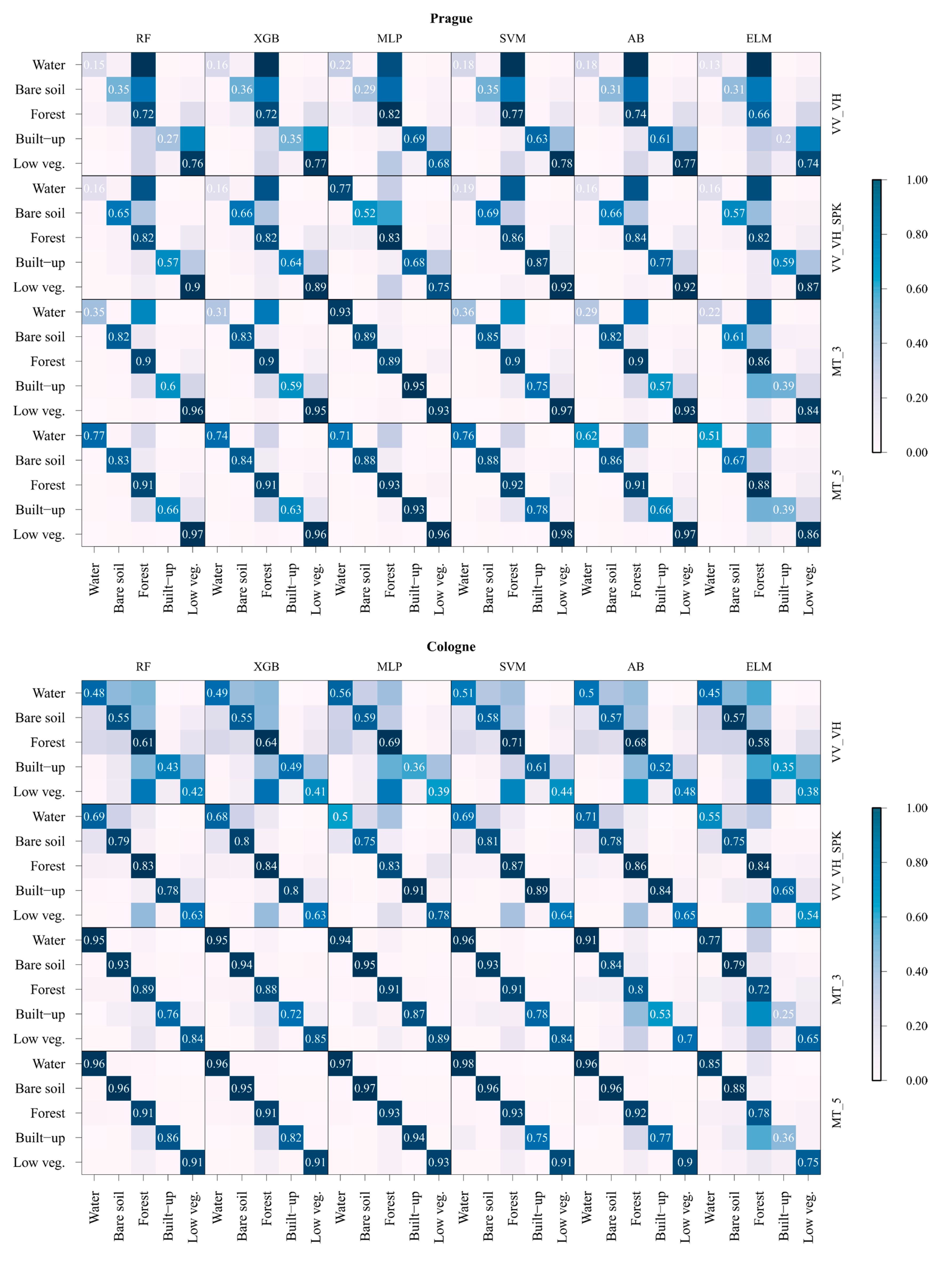
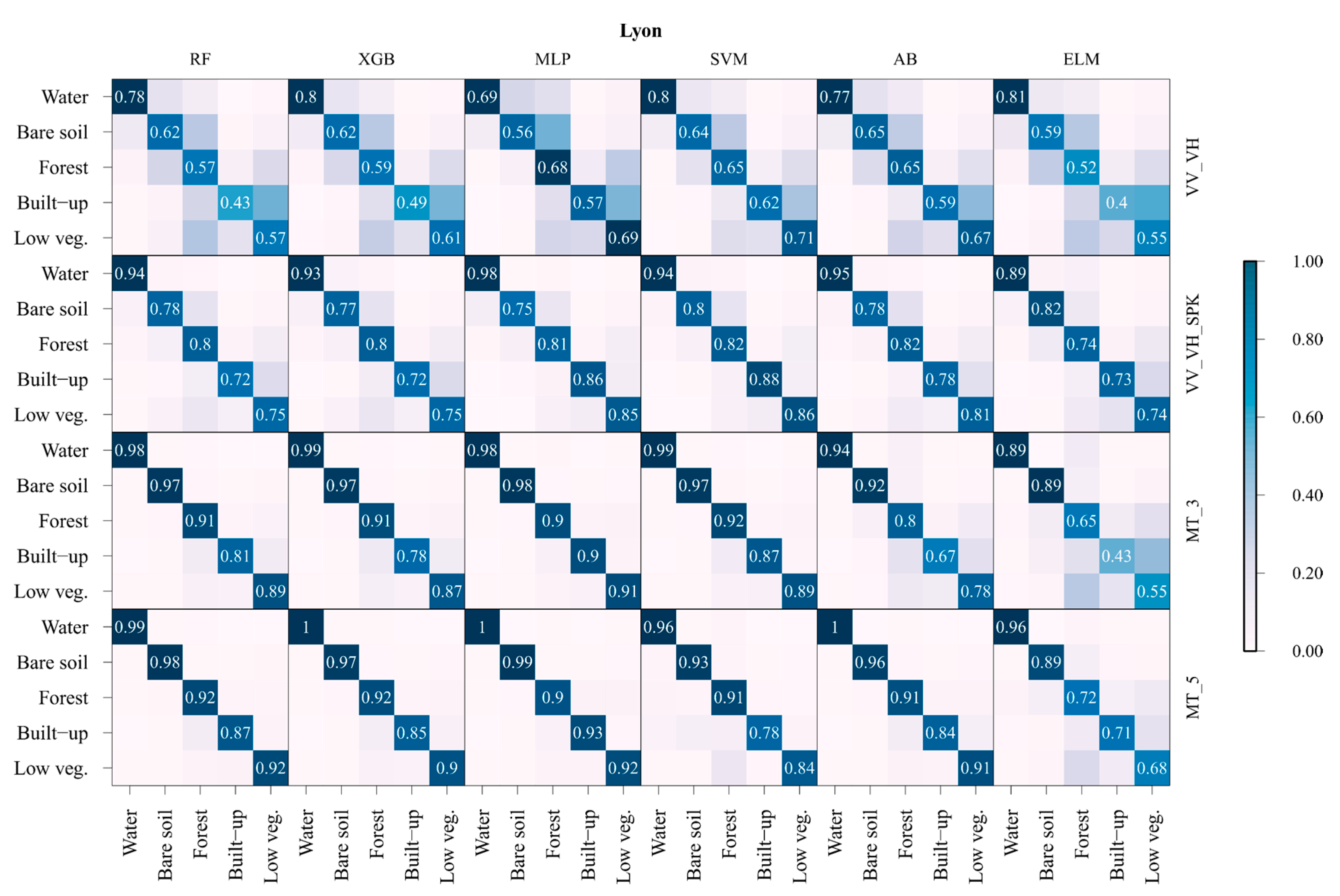
Since it is possible to obtain higher classification accuracy using an imbalanced data sets [81], macro-averaged measures (i.e., F1, FoM, UA) were used for multi-class problems because it treats all classes equally [82]. A row-wise normalization was made within each confusion matrix [83], establishing a direct comparability between matrices in the study areas of different-sized sample populations [84] (Figure 4). Elements on the main diagonal inform us how well the map represents what is really on the ground, whereas off-diagonal elements are committed (i.e., false positive error) to other land-cover classes. Therefore, Figure 4 shows an increase in the UA for different classification scenarios of this research, and with respect to the machine learning method used. LC classification using original VV and VH polarisation data shows much noise in the final results. In Prague, many areas were omitted from the correct forest category to bare soil or water class, whereas in Cologne, the lowest UA of the low vegetation class was caused by the confusion with forest, and in Lyon, built-up areas were confused with low vegetation. Commission errors decrease with speckle filtering, but still, some misclassifications using single-date imagery remain (e.g., low vegetation with forest, built-up with low vegetation), which could be improved by using MT SAR data [85]. In the MT part of the research, UA for several land-cover classes significantly improved with additional temporal S1 features. Bare land and forest classes remained with high UA values, whereas built-up areas showed some confusion with forest class. Surprisingly, a large number of forest areas were classified as a water class in Prague, although confusion between water surfaces and forests does not usually occur on SAR imagery [23,24]. At a closer visual examination of the Prague classification map and according to the historical meteorological data [86], this could be due to the rainfall event that occurred during periods of acquired imagery for two S1 imagery (i.e., 06th June and 12th June 2019). This misclassification led to an overestimation of the water category. Through the change in the medium’s dielectric constant, soil moisture had a major effect on the backscatter magnitude in terms of its increase up to 5 dB [87]. S1 MT imagery improved the classification of the low vegetation (i.e., grassland, shrubs) class, which reduced commission error with the forest and the built-up class.
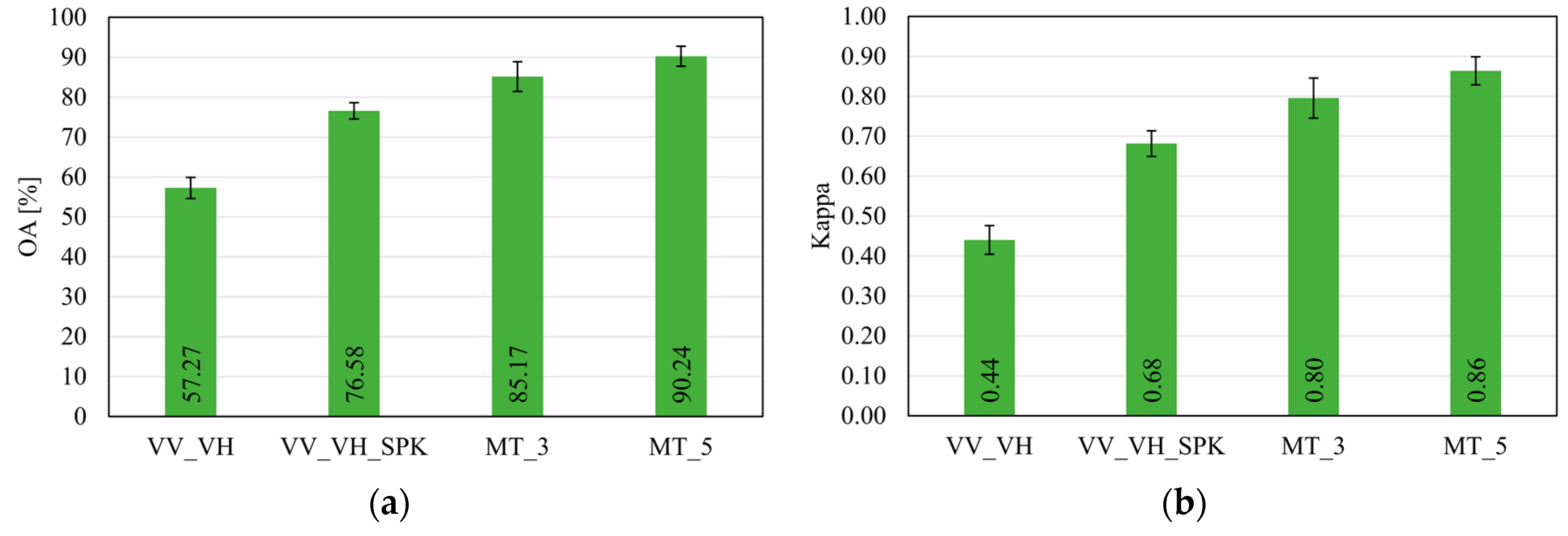
Figure 5 shows mean values for all machine learning methods evaluated in this research, with respect to the different classification scenarios. In the single-date S1 image analysis, an improvement of 20% and 0.24, in terms of the OA and Kappa values was achieved with speckle filtering. Further increase in the OA of 8.59% and 13.66% occurred with the use of three and five S1 imagery for LC classification, respectively.
In this research, the possibility of urban vegetation mapping was assessed by using various machine learning methods. In single-date image analysis, the SVM classifier achieved higher accuracy results than other classifiers (Figure 3) and the potential for detecting vegetation in built-up areas (Figure 6). In the MT classification scenario, when additional temporal information was introduced, MLP outperformed other classifiers. Therefore, Figure 6 shows a subset (2 km × 2 km) of each study area, with examples of built-up areas with surrounding urban vegetation (e.g., parks, urban gardens). Accuracy assessment was made over the entire study area (approx. 30 km × 50 km). These example subsets (Figure 6) were chosen to demonstrate the possibility of vegetation mapping in complex systems, such as urban environments, in which mixed pixels pose the greatest challenge (e.g., underestimation of the water class owing to the mixed pixels that have a subpixel land presence, as noted in [88]).
In this research, the SVM and MLP classifier achieved the highest OA and K (Figure 3) for urban vegetation mapping in the single-date (i.e., VV_VH, VV_VH_SPK), and in the MT (i.e., MT_3, MT_5) classification scenario, respectively. Therefore, McNemar’s χ2 test was statistically used to compare the classification results achieved by SVM and MLP against other classifiers for each study area (Table 5). SVM is less often wrong than any other classifier in the single-date image analysis. However, it should be noted that in some classification scenarios, SVM and AB perform very similarly. This is shown in Table 5, as the χ2 value indicates that two classifiers perform equally well with a probability of at least 95%. Using the MT SAR imagery, in Prague and Cologne, MLP achieved statistically different results from those produced by other classifiers. In Lyon, MLP yielded comparable classifications results to other classification methods, except for the ELM classifier.
5. Discussion
The current research evaluated the possibility of urban vegetation mapping using multitemporal (MT) C-band SAR imagery. Among the ML methods described in the literature [89], new machine learning methods (e.g., XGB, ELM) were tested in this research for classification tasks. Although many studies are based on the classification and interpretation of multispectral satellite imagery than those on SAR imagery, certain studies reported an increased overall classification accuracy using MT SAR imagery [85,90,91,92]. The results obtained by the tested machine learning methods confirmed that dense time-series of C-band SAR imagery allow discrimination of green and forest areas in urban systems. In this research, UA and K were used in the assessment of classification performance calculated over the entire study area (Table 1, Figure 3). Single-date image classification (i.e., VV_VH, VV_VH_SPK) was also made so that classification performance using the MT imagery could be compared (Figure 5). Using single-date data, the overall accuracy significantly increased with speckle filtering, which effectively preserved the edges and features. Similar results for LC mapping were also obtained in research by Idol et al. [80] and Lavreniuk et al. [93]. In the MT part of the research, the OA of a classification based on three (MT_3) and five (MT_5) S1 imagery was increased by 8.59% and 13.66% (Figure 5), as compared to VV_VH_SPK, respectively. By increasing the number of S1 imagery to five (MT_5), the classification accuracy further increased, and according to [85], using more than five dates for LC mapping produces negligible changes in classification accuracy. Additionally, for the MT S1 classification, a single speckle filtering was conducted rather than MT speckle filter [51], since spatial speckle filters yield a higher overall performance, as reported in [3]. Mapping of vegetation in built-up areas (i.e., forest, low vegetation) showed a better classification accuracy based on MT imagery (Table 3 and Figure 4). We used F1 and FoM accuracy metrics as macro-averaged measures that were suitable for evaluating the accuracy of various land-cover classes [69,75,94]. Table 3 shows an improvement in different classification scenarios for discriminating various land-cover classes, especially forest and low vegetation (i.e., grassland, shrubs). As suggested in [70], if omnibus measures (i.e., F1, FoM) are reported, class-specific measures should also be included to characterize the accuracy of a given class. Therefore, the UA and PA values are presented in Table 4. Large omission and commission errors occur in the VV_VH classification scenario, due to the speckle noise [80]. The errors are partly reduced with speckle filtering, but it is found that the C-band of S1 imagery is less suitable to classify vegetation classes in urban areas than, e.g., L-band [95,96]. As shown in Table 4, within sub-optimal temporal windows (i.e., classification using MT imagery), the UA and PA values increased for the individual LC classes. Similar to the previous studies [97,98], our results indicated that MT S1 imagery improved the accuracy of the vegetation mapping.
Zhu et al. [99] used Landsat and SAR data for LC classification of urban areas. For urban and forest categories, the authors recommend the usage of SAR texture measures known as GLCM (gray-level co-occurrence matrix), explained by Haralick et al. [100]. Therefore, to improve classification of the urban vegetation and green areas, the inputs to the classifiers have a more important role [29,101,102,103], than tuning the machine learning models. Haas and Ban [27] combined S1 and Sentinel-2 imagery for urban ecosystem mapping. Using an SVM classifier, 19 LC categories were mapped in complex urban areas. With the fused approach, some familiar misclassifications for SAR (classes with similar surface backscatter patterns, i.e., roads, runways, still water or lawns) and optical (classes with similar spectral reflectance) data could be reduced. Some classes are difficult to detect using a spectral response from optical data or backscatter from the SAR instrument, but this might be easily distinguished by their combined use [26,104,105]. Although F1 and FoM metrics are more robust than UA and PA [75,106], UA values, as a measure of the reliability of the map, were visualized (Figure 4) for each study area. Irrespective of the accuracy metrics used in this research, the MLP method classified the forest and low vegetation class over 90%, in the MT_5 scenario (i.e., F1, and UA).
For urban vegetation mapping, the most used machine learning methods for the classification tasks were evaluated. Urban systems are comprised of built-up areas, vegetation, and water surfaces (e.g., lakes, rivers). The example subset of Prague (Figure 6) emphasize the underestimated water extent location, due to the mixed pixels that have subpixel land presence [88]. In urban areas, these misclassifications pose a great challenge, which can be reduced by using MT imagery, or in combination with VHRSI [107,108]. Camargo et al. [46] used various machine learning methods for classifying several LC categories on ALOS-2/PALSAR-2 imagery. For nine LC classes and 200 training samples, the SVM classifier achieved the highest classification results with an OA and K of 74.18% and 0.68%, respectively. In our research, SVM also produced the best classification results in a single-date classification scenario (Figure 6), i.e., VV_VH and VV_VH_SPK, and the mean OA was 61.63% and 80.24%, respectively. The ability to apply an SVM classifier using a single SAR imagery has already been proven for LC classifications [109]. Zhong et al. [110] developed deep-learning-based LC classification for MT imagery. Similar to our research, MLP with two hidden layers and 512 neurons outperformed every non-deep learning model (i.e., XGB, RF, and SVM). Deeper MLP models did not improve the classification accuracy. In the aforementioned research, a one-dimensional convolutional neural network (CNN) achieved the highest classification results. CNNs should be further investigated for LC classification of the MT SAR imagery [111,112,113].
In this study, using MT S1 imagery for LC classification (i.e., MT_3 and MT_5), the MLP classifier achieved the highest classification results and the ability for vegetation mapping in built-up areas (Figure 6). On the contrary, ELM produced the lowest results in every classification scenario. Kernel extreme learning machine (KELM) needs to be implemented for LC classification tasks on radar and optical imagery [60,114]. The aforementioned combined use of SAR and optical imagery in MT classification tasks yields many input features (e.g., texture measures, radiometric indices), which requires a high computational capacity. Feature selection techniques should be deeply investigated in order to reduce computational cost [29,96,104,115]. We used the McNemar’s test in order to evaluate the significance of the differences between pair-wise classifications in each study area (Table 5).
6. Conclusions
In this research, we presented a comparative assessment of six machine learning methods using multitemporal (MT) SAR imagery for urban vegetation mapping. Our primary interest was to investigate the potential of S1 imagery for vegetation mapping in urban areas across Europe, since MT SAR data were not equally investigated, as compared to optical satellite data. The study revealed that discrimination of green and forest areas in urban and peri-urban areas increased with time-series of SAR imagery. Urban vegetation mapping using single-date imagery is often inefficient, and dense time-series of SAR imagery (e.g., S1) allows us to capture the phenological stages and to discriminate various land-cover classes. By using three and five S1 imagery for classification, the F1 measure for forest and low vegetation land-cover class exceeded 90%.
Furthermore, by evaluating various classification performance metrics, we selected the optimal classification method for vegetation mapping in the built-up areas. In the single-date image analysis, SVM produced the highest classification accuracy, whereas MLP yielded the best accuracy in all considered MT classification scenarios. For land-cover classification tasks using a single-date SAR imagery, SVM achieved very accurate results for even a small data set, whereas including more temporal dimensions of input data significantly improved MLP. Furthermore, mean values for all machine learning methods increased the overall classification accuracies, i.e., using three and five S1 imagery, by 49% and 58%, compared to single-date image analysis on the VV and VH bands, respectively.
This research allowed us to confirm the possibility of MT C-band SAR imagery for urban vegetation mapping. However, some deficiencies were present (e.g., mixing built-up areas with bare land or forest classes), so additional texture features or fusion with optical satellite imagery could be used along with C-band imagery. Furthermore, deep-learning classification techniques (e.g., CNN) should be thoroughly investigated for MT SAR imagery, as well as parameter optimization (e.g., k-fold cross-validation), in order to obtain the best classification performance.
Author Contributions
Conceptualization, M.G.; investigation, M.G. and D.D.; methodology, M.G. and D.D.; supervision, M.G.; validation, M.G. and D.D.; visualization, M.G.; writing–original draft, M.G. and D.D.; writing–review & editing, M.G. All authors have read and agreed to the published version of the manuscript.
Funding
This work was supported by the Croatian Science Foundation for the GEMINI project: “Geospatial Monitoring of Green Infrastructure by Means of Terrestrial, Airborne and Satellite Imagery” (Grant No. HRZZ-IP-2016-06-5621); and the University of Zagreb for the project: “Advanced photogrammetry and remote sensing methods for environmental change monitoring” (Grant No. RS4ENVIRO).
Conflicts of Interest
The authors declare no conflict of interest.
Appendix A

Table A1.
Detailed characteristics of the study areas used in this research.
| Study Area | Prague | Cologne | Lyon |
|---|---|---|---|
| Country | Czech Republic | Germany | France |
| Lat/Long | 50°5′ N | 50°56′ N | 45°45′ N |
| 14°25′ E | 6°57′ E | 4°50′ E | |
| Extent (pixels) | 4958 × 3038 | 5213 × 3151 | 5145 × 3344 |
| Climate | Humid continental | Temperate oceanic | Temperate oceanic |
| Average annual | max. 14.9 | max. 16.5 | max. 18.2 |
| temperature (°C) | mean 12.6 | mean 13.9 | mean 14.8 |
| −2019 * | min. 7.5 | min. 9.3 | min. 9.6 |
| Precipitation (mm) | 984.0 | 979.1 | 1524.6 |
| −2019 * | |||
| Soils ** | Haplic Chernozems | Orthic Luvisols | Vertic Luvisols |
* Data collected at WorldWeatherOnline.com; ** Information about soils extracted from FAO–UNESCO [116].
References
- Gomez-Chova, L.; Fernández-Prieto, D.; Calpe, J.; Soria, E.; Vila, J.; Camps-Valls, G. Urban monitoring using multi-temporal SAR and multi-spectral data. Pattern Recognit. Lett. 2006, 27, 234–243. [Google Scholar] [CrossRef]
- Blaschke, T.; Hay, G.J.; Weng, Q.; Resch, B. Collective Sensing: Integrating Geospatial Technologies to Understand Urban Systems—An Overview. Remote Sens. 2011, 3, 1743–1776. [Google Scholar] [CrossRef] [Green Version]
- Maghsoudi, Y.; Collins, M.J.; Leckie, D. Speckle reduction for the forest mapping analysis of multi-temporal Radarsat-1 images. Int. J. Remote Sens. 2012, 33, 1349–1359. [Google Scholar] [CrossRef]
- Skriver, H. Crop classification by multitemporal C- and L-band single- and dual-polarization and fully polarimetric SAR. IEEE Trans. Geosci. Remote Sens. 2012, 50, 2138–2149. [Google Scholar] [CrossRef]
- Moreira, A.; Prats-iraola, P.; Younis, M.; Krieger, G.; Hajnsek, I.; Papathanassiou, K.P. A tutorial on synthetic aperture radar. IEEE Geosci. Remote Sens. Mag. 2013, 1, 6–43. [Google Scholar] [CrossRef] [Green Version]
- Oliver, C.J. Information from SAR images. J. Phys. D Appl. Phys. 1991, 24, 1493–1514. [Google Scholar] [CrossRef] [Green Version]
- Yuan, J.; Lv, X.; Li, R. A speckle filtering method based on hypothesis testing for time-series SAR images. Remote Sens. 2018, 10, 1383. [Google Scholar] [CrossRef] [Green Version]
- Frost, V.S.; Stiles, J.A.; Shanmugan, K.S.; Holtzman, J.C. A Model for Radar Images and Its Application to Adaptive Digital Filtering of Multiplicative Noise. IEEE Trans. Pattern Anal. Mach. Intell. 1982, 2, 157–166. [Google Scholar] [CrossRef]
- Kuan, D.T.; Sawchuk, A.A.; Strand, T.C.; Chavel, P. Adaptive Restoration of Images with Speckle. IEEE Trans. Acoust. 1987, 35, 373–383. [Google Scholar] [CrossRef]
- Lee, J. Sen Digital image smoothing and the sigma filter. Comput. Vis. Graph. Image Process. 1983, 24, 255–269. [Google Scholar] [CrossRef]
- Lee, J. Sen Digital Image Enhancement and Noise Filtering by Use of Local Statistics. IEEE Trans. Pattern Anal. Mach. Intell. 1980, 2, 165–168. [Google Scholar] [CrossRef] [Green Version]
- Lopes, A.; Nezry, E.; Touzi, R.; Laur, H. Maximum a posteriori speckle filtering and first order texture models in SAR images. In Proceedings of the 10th Annual International Symposium on Geoscience and Remote Sensing, College Park, MD, USA, 20–24 May 1990; IEEE: Piscataway, NJ, USA, 1990; pp. 2409–2412. [Google Scholar] [CrossRef]
- Xiao, J.; Li, J.; Moody, A. A detail-preserving and flexible adaptive filter for speckle suppression in SAR imagery. Int. J. Remote Sens. 2003, 24, 2451–2465. [Google Scholar] [CrossRef]
- Guerschman, J.P.; Paruelo, J.M.; Di Bella, C.; Giallorenzi, M.C.; Pacin, F. Land cover classification in the Argentine Pampas using multi-temporal Landsat TM data. Int. J. Remote Sens. 2003, 24, 3381–3402. [Google Scholar] [CrossRef]
- Martinez, J.M.; Le Toan, T. Mapping of flood dynamics and spatial distribution of vegetation in the Amazon floodplain using multitemporal SAR data. Remote Sens. Environ. 2007, 108, 209–223. [Google Scholar] [CrossRef]
- Quegan, S.; Le Toan, T.; Yu, J.J.; Ribbes, F.; Floury, N. Multitemporal ERS SAR analysis applied to forest mapping. IEEE Trans. Geosci. Remote Sens. Environ. 2000, 38, 741–753. [Google Scholar] [CrossRef]
- Townsend, P.A. Estimating forest structure in wetlands using multitemporal SAR. Remote Sens. Environ. 2002, 79, 288–304. [Google Scholar] [CrossRef]
- Waske, B.; Heinzel, V.; Braun, M.; Menz, G. Random forests for classifying multi-temporal SAR data. In Proceedings of the Envisat Symposium 2007, Montreux, Switzerland, 23–27 April 2007; pp. 1–4. [Google Scholar]
- Veloso, A.; Mermoz, S.; Bouvet, A.; Le Toan, T.; Planells, M.; Dejoux, J.F.; Ceschia, E. Understanding the temporal behavior of crops using Sentinel-1 and Sentinel-2-like data for agricultural applications. Remote Sens. Environ. 2017, 199, 415–426. [Google Scholar] [CrossRef]
- Vreugdenhil, M.; Wagner, W.; Bauer-Marschallinger, B.; Pfeil, I.; Teubner, I.; Rüdiger, C.; Strauss, P. Sensitivity of Sentinel-1 Backscatter to Vegetation Dynamics: An Austrian Case Study. Remote Sens. 2018, 10, 1396. [Google Scholar] [CrossRef] [Green Version]
- Gao, Q.; Zribi, M.; Escorihuela, M.J.; Baghdadi, N.; Segui, P.Q. Irrigation mapping using Sentinel-1 time series at field scale. Remote Sens. 2018, 10, 1495. [Google Scholar] [CrossRef] [Green Version]
- Amitrano, D.; Di Martino, G.; Iodice, A.; Riccio, D.; Ruello, G. Unsupervised Rapid Flood Mapping Using Sentinel-1 GRD SAR Images. IEEE Trans. Geosci. Remote Sens. 2018, 56, 3290–3299. [Google Scholar] [CrossRef]
- Tsyganskaya, V.; Martinis, S.; Marzahn, P.; Ludwig, R. Detection of temporary flooded vegetation using Sentinel-1 time series data. Remote Sens. 2018, 10, 1286. [Google Scholar] [CrossRef] [Green Version]
- Twele, A.; Cao, W.; Plank, S.; Martinis, S. Sentinel-1-based flood mapping: A fully automated processing chain. Int. J. Remote Sens. 2016, 37, 2990–3004. [Google Scholar] [CrossRef]
- Tsyganskaya, V.; Martinis, S.; Marzahn, P.; Ludwig, R. SAR-based detection of flooded vegetation–a review of characteristics and approaches. Int. J. Remote Sens. 2018, 39, 2255–2293. [Google Scholar] [CrossRef]
- Joshi, N.; Baumann, M.; Ehammer, A.; Fensholt, R.; Grogan, K.; Hostert, P.; Jepsen, M.R.; Kuemmerle, T.; Meyfroidt, P.; Mitchard, E.T.A.; et al. A Review of the Application of Optical and Radar Remote Sensing Data Fusion to Land Use Mapping and Monitoring. Remote Sens. 2016, 8, 70. [Google Scholar] [CrossRef] [Green Version]
- Haas, J.; Ban, Y. Sentinel-1A SAR and sentinel-2A MSI data fusion for urban ecosystem service mapping. Remote Sens. Appl. Soc. Environ. 2017, 8, 41–53. [Google Scholar] [CrossRef]
- Jacob, A.; Ban, Y. Sentinel-1A SAR Data for Global Urban Mapping: Preliminary Results. In Proceedings of the 2015 IEEE International on Geoscience and Remote Sensing Symposium (IGARSS), Milan, Italy, 26–31 July 2015; pp. 1179–1182. [Google Scholar] [CrossRef]
- Tavares, P.A.; Beltrão, N.E.S.; Guimarães, U.S.; Teodoro, A.C. Integration of sentinel-1 and sentinel-2 for classification and LULC mapping in the urban area of Belém, eastern Brazilian Amazon. Sensors 2019, 19, 1140. [Google Scholar] [CrossRef] [Green Version]
- Du, P.; Li, X.; Cao, W.; Luo, Y.; Zhang, H. Monitoring urban land cover and vegetation change by multi-temporal remote sensing information. Min. Sci. Technol. 2010, 20, 922–932. [Google Scholar] [CrossRef]
- Gašparović, M.; Dobrinić, D.; Medak, D. Urban Vegetation Detection Based on the Land-Cover Classification of Planetscope, Rapideye and Worldview-2 Satellite Imagery. In Proceedings of the 18th International Multidisciplinary Scientific Geo-Conference SGEM2018, Albena, Bulgaria, 30 June–9 July 2018; pp. 249–256. [Google Scholar] [CrossRef] [Green Version]
- Shade, C.; Kremer, P. Predicting Land Use Changes in Philadelphia Following Green Infrastructure Policies. Land 2019, 8, 28. [Google Scholar] [CrossRef] [Green Version]
- Sonobe, R. Parcel-Based Crop Classification Using Multi-Temporal TerraSAR-X Dual Polarimetric Data. Remote Sens. 2019, 11, 1148. [Google Scholar] [CrossRef] [Green Version]
- Zhang, Y.; Wang, C.; Wu, J.; Qi, J.; Salas, W.A. Mapping paddy rice with multitemporal ALOS/PALSAR imagery in southeast China. Int. J. Remote Sens. 2009, 30, 6301–6315. [Google Scholar] [CrossRef]
- Han, M.; Zhu, X.; Yao, W. Remote sensing image classification based on neural network ensemble algorithm. Neurocomputing 2012, 78, 133–138. [Google Scholar] [CrossRef]
- Kussul, N.; Lavreniuk, M.; Skakun, S.; Shelestov, A. Deep Learning Classification of Land Cover and Crop Types Using Remote Sensing Data. IEEE Geosci. Remote Sens. Lett. 2017, 14, 778–782. [Google Scholar] [CrossRef]
- Nyoungui, A.N.; Tonye, E.; Akono, A. Evaluation of speckle filtering and texture analysis methods for land cover classification from SAR images. Int. J. Remote Sens. 2002, 23, 1895–1925. [Google Scholar] [CrossRef]
- Chen, T.; Guestrin, C. XGBoost: A Scalable Tree Boosting System. In Proceedings of the 22nd ACM SIGKDD International Conference on Knowledge Discovery and Data Mining, San Francisco, CA, USA, 13–17 August 2016; pp. 785–794. [Google Scholar]
- Freund, Y.; Schapire, R.E. Experiments with a New Boosting Algorithm. In Proceedings of the Thirteenth International Conference on International Conference on Machine Learning, Bari, Italy, 3–6 July 1996; Morgan Kaufmann Publishers Inc.: San Francisco, CA, USA, 1996; pp. 148–156. [Google Scholar]
- Chen, Y.; Dou, P.; Yang, X. Improving land use/cover classification with a multiple classifier system using AdaBoost integration technique. Remote Sens. 2017, 9, 1055. [Google Scholar] [CrossRef] [Green Version]
- Kulkarni, S.; Kelkar, V. Classification of multispectral satellite images using ensemble techniques of bagging, boosting and adaboost. In Proceedings of the International Conference on Circuits, Systems, Communication and Information Technology Applications (CSCITA) Classification, Mumbai, India, 4–5 April 2014; pp. 253–258. [Google Scholar]
- Kawaguchi, S.; Nishii, R. Hyperspectral image classification by bootstrap AdaBoost with random decision stumps. IEEE Trans. Geosci. Remote Sens. 2007, 45, 3845–3851. [Google Scholar] [CrossRef]
- Khosravi, I.; Mohammad-Beigi, M. Multiple Classifier Systems for Hyperspectral Remote Sensing Data Classification. J. Indian Soc. Remote Sens. 2014, 42, 423–428. [Google Scholar] [CrossRef]
- Huang, G.B.; Zhu, Q.Y.; Siew, C.K. Extreme learning machine: Theory and applications. Neurocomputing 2006, 70, 489–501. [Google Scholar] [CrossRef]
- Pal, M. Extreme-learning-machine-based land cover classification. Int. J. Remote Sens. 2009, 30, 3835–3841. [Google Scholar] [CrossRef] [Green Version]
- Camargo, F.F.; Sano, E.E.; Almeida, C.M.; Mura, J.C.; Almeida, T. A comparative assessment of machine-learning techniques for land use and land cover classification of the Brazilian tropical savanna using ALOS-2/PALSAR-2 polarimetric images. Remote Sens. 2019, 11, 1600. [Google Scholar] [CrossRef] [Green Version]
- Lapini, A.; Pettinato, S.; Santi, E.; Paloscia, S.; Fontanelli, G.; Garzelli, A. Comparison of Machine Learning Methods Applied to SAR Images for Forest Classification in Mediterranean Areas. Remote Sens. 2020, 12, 369. [Google Scholar] [CrossRef] [Green Version]
- Waske, B.; Braun, M. Classifier ensembles for land cover mapping using multitemporal SAR imagery. ISPRS J. Photogramm. Remote Sens. 2009, 64, 450–457. [Google Scholar] [CrossRef]
- Lee, J.S.; Jurkevich, I.; Dewaele, P.; Wambacq, P.; Oosterlinck, A. Speckle filtering of synthetic aperture radar images: A review. Remote Sens. Rev. 1994, 8, 313–340. [Google Scholar] [CrossRef]
- Wang, X.; Ge, L.; Li, X. Evaluation of Filters for Envisat Asar Speckle Suppression in Pasture Area. ISPRS Ann. Photogramm. Remote Sens. Spat. Inf. Sci. 2012, 1, 341–346. [Google Scholar] [CrossRef] [Green Version]
- Quegan, S.; Yu, J.J. Filtering of multichannel SAR images. IEEE Trans. Geosci. Remote Sens. 2001, 39, 2373–2379. [Google Scholar] [CrossRef]
- McNairn, H.; Kross, A.; Lapen, D.; Caves, R.; Shang, J. Early season monitoring of corn and soybeans with TerraSAR-X and RADARSAT-2. Int. J. Appl. Earth Obs. Geoinf. 2014, 28, 252–259. [Google Scholar] [CrossRef]
- Breiman, L. Random forests. Mach. Learn. 2001, 45, 5–32. [Google Scholar] [CrossRef] [Green Version]
- Noi, P.T.; Kappas, M. Comparison of random forest, k-nearest neighbor, and support vector machine classifiers for land cover classification using sentinel-2 imagery. Sensors 2018, 18, 18. [Google Scholar] [CrossRef] [Green Version]
- Liaw, A.; Wiener, M. Classification and Regression by randomForest. R News 2002, 2, 18–22. [Google Scholar]
- Qian, Y.; Zhou, W.; Yan, J.; Li, W.; Han, L. Comparing Machine Learning Classifiers for Object-Based Land Cover Classification Using Very High Resolution Imagery. Remote Sens. 2015, 7, 153–168. [Google Scholar] [CrossRef]
- Karatzoglou, A.; Smola, A.; Hornik, K.; Zeileis, A. kernlab-An S4 Package for Kernel Methods in R. J. Stat. Softw. 2004, 11, 1–20. [Google Scholar] [CrossRef] [Green Version]
- Chen, T.; He, T.; Benesty, M.; Khotilovich, V.; Tang, Y.; Cho, H.; Chen, K.; Mitchell, R.; Cano, I.; Zhou, T.; et al. Xgboost: Extreme Gradient Boosting, R Package Version 0.82.1. Available online: https://CRAN.R-project.org/package=xgboost (accessed on 30 May 2020).
- Man, C.D.; Nguyen, T.T.; Bui, H.Q.; Lasko, K.; Nguyen, T.N.T. Improvement of land-cover classification over frequently cloud-covered areas using landsat 8 time-series composites and an ensemble of supervised classifiers. Int. J. Remote Sens. 2018, 39, 1243–1255. [Google Scholar] [CrossRef]
- Sonobe, R.; Yamaya, Y.; Tani, H.; Wang, X.; Kobayashi, N.; Mochizuki, K.I. Assessing the suitability of data from Sentinel-1A and 2A for crop classification. GISci. Remote Sens. 2017, 54, 918–938. [Google Scholar] [CrossRef]
- Allaire, J.J.; Chollet, F. Keras: R Interface to ‘Keras’, R Package Version 2.2.4.1. Available online: https://CRAN.R-project.org/package=keras (accessed on 30 May 2020).
- Heaton, J. Introduction to Neural Networks with Java, 2nd ed.; Heaton Research, Inc.: Chesterfield, MO, USA, 2008. [Google Scholar]
- Zhang, C.; Sargent, I.; Pan, X.; Li, H.; Gardiner, A.; Hare, J.; Atkinson, P.M. Joint Deep Learning for land cover and land use classification. Remote Sens. Environ. 2019, 221, 173–187. [Google Scholar] [CrossRef] [Green Version]
- Alfaro, E.; Gáamez, M.; García, N. Adabag: An R package for classification with boosting and bagging. J. Stat. Softw. 2013, 54, 1–35. [Google Scholar] [CrossRef] [Green Version]
- Mouselimis, L.; Gosso, A. elmNNRcpp: The Extreme Learning Machine Algorithm, R Package Version 1.0.1. Available online: https://CRAN.R-project.org/package=elmNNRcpp (accessed on 30 May 2020).
- Olofsson, P.; Foody, G.M.; Herold, M.; Stehman, S.V.; Woodcock, C.E.; Wulder, M.A. Good practices for estimating area and assessing accuracy of land change. Remote Sens. Environ. 2014, 148, 42–57. [Google Scholar] [CrossRef]
- Stehman, S.V. Sampling designs for accuracy assessment of land cover. Int. J. Remote Sens. 2009, 30, 5243–5272. [Google Scholar] [CrossRef]
- Ottinger, M.; Clauss, K.; Kuenzer, C. Large-scale assessment of coastal aquaculture ponds with Sentinel-1 time series data. Remote Sens. 2017, 9, 440. [Google Scholar] [CrossRef] [Green Version]
- Gašparović, M.; Jogun, T. The effect of fusing Sentinel-2 bands on land-cover classification. Int. J. Remote Sens. 2018, 39, 822–841. [Google Scholar] [CrossRef]
- Stehman, S.V.; Foody, G.M. Key issues in rigorous accuracy assessment of land cover products. Remote Sens. Environ. 2019, 231, 111199. [Google Scholar] [CrossRef]
- Valero, S.; Morin, D.; Inglada, J.; Sepulcre, G.; Arias, M.; Hagolle, O.; Dedieu, G.; Bontemps, S.; Defourny, P.; Koetz, B. Production of a Dynamic Cropland Mask by Processing Remote Sensing Image Series at High Temporal and Spatial Resolutions. Remote Sens. 2016, 8, 55. [Google Scholar] [CrossRef] [Green Version]
- Pal, M.; Mather, P.M. Support vector machines for classification in remote sensing. Int. J. Remote Sens. 2005, 26, 1007–1011. [Google Scholar] [CrossRef]
- Story, M.; Congalton, R.G. Remote Sensing Brief Accuracy Assessment: A User’s Perspective. Photogramm. Eng. Remote Sens. 1986, 52, 397–399. [Google Scholar]
- Jäger, G.; Benz, U. Measures of classification accuracy based on fuzzy similarity. IEEE Trans. Geosci. Remote Sens. 2000, 38, 1462–1467. [Google Scholar] [CrossRef]
- Sun, C.; Bian, Y.; Zhou, T.; Pan, J. Using of multi-source and multi-temporal remote sensing data improves crop-type mapping in the subtropical agriculture region. Sensors 2019, 19, 2401. [Google Scholar] [CrossRef] [Green Version]
- Pontius, R.G.; Millones, M. Death to Kappa: Birth of quantity disagreement and allocation disagreement for accuracy assessment. Int. J. Remote Sens. 2011, 32, 4407–4429. [Google Scholar] [CrossRef]
- Colditz, R.R. An evaluation of different training sample allocation schemes for discrete and continuous land cover classification using decision tree-based algorithms. Remote Sens. 2015, 7, 9655–9681. [Google Scholar] [CrossRef] [Green Version]
- McNemar, Q. Note on the sampling error of the difference between correlated proportions or percentages. Psychometrika 1947, 12, 153–157. [Google Scholar] [CrossRef]
- Whyte, A.; Ferentinos, K.P.; Petropoulos, G.P. A new synergistic approach for monitoring wetlands using Sentinels -1 and 2 data with object-based machine learning algorithms. Environ. Model. Softw. 2018, 104, 40–54. [Google Scholar] [CrossRef] [Green Version]
- Idol, T.; Haack, B.; Mahabir, R. Radar speckle reduction and derived texture measures for land cover/use classification: A case study. Geocarto Int. 2017, 32, 18–29. [Google Scholar] [CrossRef]
- Abdi, A.M. Land cover and land use classification performance of machine learning algorithms in a boreal landscape using Sentinel-2 data. GISci. Remote Sens. 2019, 57, 1–20. [Google Scholar] [CrossRef] [Green Version]
- Sokolova, M.; Lapalme, G. A systematic analysis of performance measures for classification tasks. Inf. Process. Manag. 2009, 45, 427–437. [Google Scholar] [CrossRef]
- Markert, K.N.; Griffin, R.E.; Limaye, A.S.; McNider, R.T. Spatial Modeling of Land Cover/Land Use Change and Its Effects on Hydrology Within the Lower Mekong Basin. In Land Atmospheric Research Applications in Asia; Vadrevu, K.P., Ohara, T., Justice, C., Eds.; Springer: Heidelberg/Berlin, Germany, 2018; pp. 667–698. [Google Scholar]
- Stehman, S.V. A critical evaluation of the normalized error matrix in map accuracy assessment. Photogramm. Eng. Remote Sens. 2004, 70, 743–751. [Google Scholar] [CrossRef]
- Chust, G.; Ducrot, D.; Pretus, J.L. Land cover discrimination potential of radar multitemporal series and optical multispectral images in a Mediterranean cultural landscape. Int. J. Remote Sens. 2004, 25, 3513–3528. [Google Scholar] [CrossRef]
- CHMI Portal—Meteorological Measurements at Prague’s Clementinum Observatory. Available online: http://portal.chmi.cz/historicka-data/pocasi/praha-klementinum?l=en (accessed on 30 May 2020).
- Molijn, R.; Iannini, L.; López Dekker, P.; Magalhães, P.; Hanssen, R. Vegetation Characterization through the Use of Precipitation-Affected SAR Signals. Remote Sens. 2018, 10, 1647. [Google Scholar] [CrossRef] [Green Version]
- Kim, S.; Brisco, B.; Poncos, V. Boreal Inundation Mapping with SMAP Radiometer Data for Methane Studies. In Proceedings of the 19th EGU General Assembly (EGU 2017), Vienna, Austria, 23–28 April 2017; p. 10916. [Google Scholar]
- Maxwell, A.E.; Warner, T.A.; Fang, F. Implementation of machine-learning classification in remote sensing: An applied review. Int. J. Remote Sens. 2018, 39, 2784–2817. [Google Scholar] [CrossRef] [Green Version]
- Demarez, V.; Helen, F.; Marais-Sicre, C.; Baup, F. In-Season Mapping of Irrigated Crops Using Landsat 8 and Sentinel-1 Time Series. Remote Sens. 2019, 11, 118. [Google Scholar] [CrossRef] [Green Version]
- Park, S.; Im, J.; Park, S.; Yoo, C.; Han, H.; Rhee, J. Classification and Mapping of Paddy Rice by Combining Landsat and SAR Time Series Data. Remote Sens. 2018, 10, 447. [Google Scholar] [CrossRef] [Green Version]
- Skriver, H.; Mattia, F.; Satalino, G.; Balenzano, A.; Pauwels, V.R.N.; Verhoest, N.E.C.; Davidson, M. Crop Classification Using Short-Revisit Multitemporal SAR Data. IEEE J. Sel. Top. Appl. Earth Obs. Remote Sens. 2011, 4, 423–431. [Google Scholar] [CrossRef]
- Lavreniuk, M.; Kussul, N.; Meretsky, M.; Lukin, V.; Abramov, S.; Rubel, O. Impact of SAR data filtering on crop classification accuracy. In Proceedings of the 2017 IEEE First Ukraine Conference on Electrical and Computer Engineering (UKRCON), Kiev, Ukraine, 29 May–2 June 2017; pp. 912–917. [Google Scholar] [CrossRef]
- Remelgado, R.; Safi, K.; Wegmann, M. From ecology to remote sensing: Using animals to map land cover. Remote Sens. Ecol. Conserv. 2020, 6, 93–104. [Google Scholar] [CrossRef]
- Patel, P.; Srivastava, H.S.; Panigrahy, S.; Parihar, J.S. Comparative evaluation of the sensitivity of multi-polarized multi-frequency SAR backscatter to plant density. Int. J. Remote Sens. 2006, 27, 293–305. [Google Scholar] [CrossRef]
- Mercier, A.; Betbeder, J.; Rumiano, F.; Baudry, J.; Gond, V.; Blanc, L.; Bourgoin, C.; Cornu, G.; Ciudad, C.; Marchamalo, M.; et al. Evaluation of Sentinel-1 and 2 Time Series for Land Cover Classification of Forest–Agriculture Mosaics in Temperate and Tropical Landscapes. Remote Sens. 2019, 11, 979. [Google Scholar] [CrossRef] [Green Version]
- Niculescu, S.; Talab Ou Ali, H.; Billey, A. Random forest classification using Sentinel-1 and Sentinel-2 series for vegetation monitoring in the Pays de Brest (France). In Proceedings of the SPIE—Remote Sensing for Agriculture, Ecosystems, and Hydrology XX, Berlin, Germany, 10–13 September 2018; Volume 10783, pp. 1–18. [Google Scholar] [CrossRef]
- Liu, Y.; Gong, W.; Hu, X.; Gong, J. Forest type identification with random forest using Sentinel-1A, Sentinel-2A, multi-temporal Landsat-8 and DEM data. Remote Sens. 2018, 10, 946. [Google Scholar] [CrossRef] [Green Version]
- Zhu, Z.; Woodcock, C.E.; Rogan, J.; Kellndorfer, J. Assessment of spectral, polarimetric, temporal, and spatial dimensions for urban and peri-urban land cover classification using Landsat and SAR data. Remote Sens. Environ. 2012, 117, 72–82. [Google Scholar] [CrossRef]
- Haralick, R.M.; Shanmugam, K.; Dinstein, I. Textural Features for Image Classification. IEEE Trans. Syst. Man Cybern. 1973, 3, 610–621. [Google Scholar] [CrossRef] [Green Version]
- Balzter, H.; Cole, B.; Thiel, C.; Schmullius, C. Mapping CORINE land cover from Sentinel-1A SAR and SRTM digital elevation model data using random forests. Remote Sens. 2015, 7, 14876–14898. [Google Scholar] [CrossRef] [Green Version]
- Pesaresi, M.; Corbane, C.; Julea, A.; Florczyk, A.; Syrris, V.; Soille, P.; Pesaresi, M.; Corbane, C.; Julea, A.; Florczyk, A.J.; et al. Assessment of the Added-Value of Sentinel-2 for Detecting Built-up Areas. Remote Sens. 2016, 8, 299. [Google Scholar] [CrossRef] [Green Version]
- Zakeri, H.; Yamazaki, F.; Liu, W. Texture Analysis and Land Cover Classification of Tehran Using Polarimetric Synthetic Aperture Radar Imagery. Appl. Sci. 2017, 7, 452. [Google Scholar] [CrossRef] [Green Version]
- Jin, Y.; Liu, X.; Chen, Y.; Liang, X. Land-cover mapping using Random Forest classification and incorporating NDVI time-series and texture: A case study of central Shandong. Int. J. Remote Sens. 2018, 39, 8703–8723. [Google Scholar] [CrossRef]
- Pavanelli, J.A.P.; dos Santos, J.R.; Galvão, L.S.; Xaud, M.R.; Xaud, H.A.M. Palsar-2/ALOS-2 and Oli/Landsat-8 data integration for land use and land cover mapping in northern Brazilian Amazon. Bol. Cienc. Geod. 2018, 24, 250–269. [Google Scholar] [CrossRef]
- Schuster, C.; Schmidt, T.; Conrad, C.; Kleinschmit, B.; Förster, M. Grassland habitat mapping by intra-annual time series analysis-Comparison of RapidEye and TerraSAR-X satellite data. Int. J. Appl. Earth Obs. Geoinf. 2015, 34, 25–34. [Google Scholar] [CrossRef]
- Xing, L.; Tang, X.; Wang, H.; Fan, W.; Wang, G. Monitoring monthly surface water dynamics of Dongting Lake using Sentinel-1 data at 10 m. PeerJ 2018, 6, e4992. [Google Scholar] [CrossRef]
- Kuenzer, C.; Guo, H.; Schlegel, I.; Tuan, V.Q.; Li, X.; Dech, S. Varying Scale and Capability of Envisat ASAR-WSM, TerraSAR-X Scansar and TerraSAR-X Stripmap Data to Assess Urban Flood Situations: A Case Study of the Mekong Delta in Can Tho Province. Remote Sens. 2013, 5, 5122–5142. [Google Scholar] [CrossRef] [Green Version]
- Clerici, N.; Valbuena Calderón, C.A.; Posada, J.M. Fusion of sentinel-1a and sentinel-2A data for land cover mapping: A case study in the lower Magdalena region, Colombia. J. Maps 2017, 13, 718–726. [Google Scholar] [CrossRef] [Green Version]
- Zhong, L.; Hu, L.; Zhou, H. Deep learning based multi-temporal crop classification. Remote Sens. Environ. 2019, 221, 430–443. [Google Scholar] [CrossRef]
- Ho Tong Minh, D.; Ienco, D.; Gaetano, R.; Lalande, N.; Ndikumana, E.; Osman, F.; Maurel, P. Deep Recurrent Neural Networks for Winter Vegetation Quality Mapping via Multitemporal SAR Sentinel-1. IEEE Geosci. Remote Sens. Lett. 2018, 15, 465–468. [Google Scholar] [CrossRef]
- Kamilaris, A.; Prenafeta-Boldú, F.X. Deep learning in agriculture: A survey. Comput. Electron. Agric. 2018, 147, 70–90. [Google Scholar] [CrossRef] [Green Version]
- Mullissa, A.G.; Persello, C.; Tolpekin, V. Fully convolutional networks for multi-temporal SAR image classification. In Proceedings of the IGARSS 2018-2018 IEEE International Geoscience and Remote Sensing Symposium, Valencia, Spain, 22–27 July 2018; pp. 6635–6638. [Google Scholar] [CrossRef]
- Sonobe, R.; Tani, H.; Wang, X. An experimental comparison between KELM and CART for crop classification using Landsat-8 OLI data. Geocarto Int. 2016, 32, 128–138. [Google Scholar] [CrossRef] [Green Version]
- Inglada, J.; Vincent, A.; Arias, M.; Marais-Sicre, C. Improved early crop type identification by joint use of high temporal resolution sar and optical image time series. Remote Sens. 2016, 8, 362. [Google Scholar] [CrossRef] [Green Version]
- FAO-UNESCO. Soil Map of the World 1:5000000; UNESCO: Paris, France, 1981; Volume 5, ISBN 92-3-101364-0. [Google Scholar]
Figure 1.
The number of published articles (1990–2019) listed in the Web of Science Core Collection containing the terms/topic “radar” or “scatteromet*” or “microwave*” or “SAR” for radar, and “optic*” or “Landsat” or “Sentinel-2” or “Sentinel-3” or “Quickbird” or “MODIS” or “IKONOS” or “GeoEye” or “WorldView” for optical imagery, refined by “land cover” or “land use”. To extract a number of multitemporal related articles, the final results were refined by “multitemporal” or “multi-temporal” or “multi temporal” or “time-series” or “time series”.
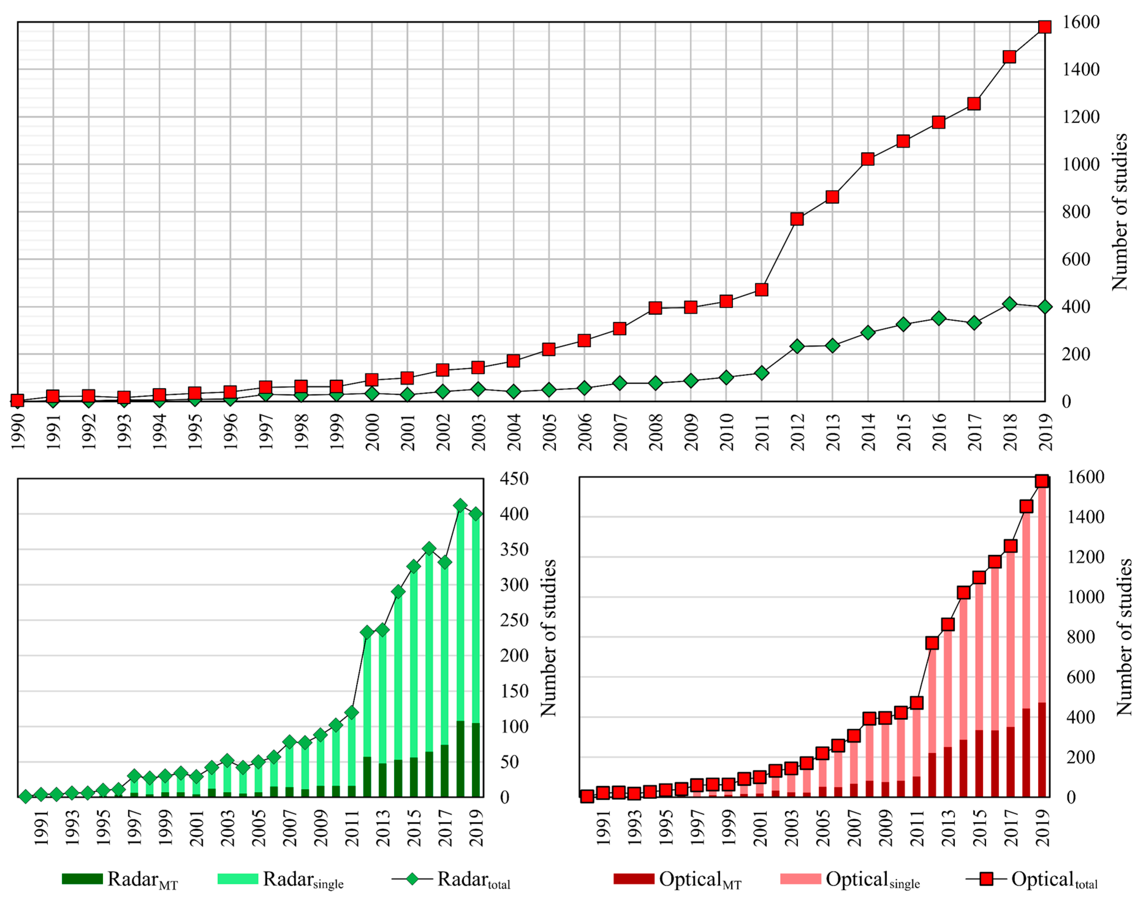
Figure 2.
(a) Locations across Europe used in this research; (b); (c); and (d) show the study areas located in Prague; Cologne; and Lyon, respectively, whereas the red square represents an example subset location for a classification map, with an extent of 2 km × 2 km.
Figure 2.
(a) Locations across Europe used in this research; (b); (c); and (d) show the study areas located in Prague; Cologne; and Lyon, respectively, whereas the red square represents an example subset location for a classification map, with an extent of 2 km × 2 km.

Figure 3.
Mean (a) OA and (b) Kappa values obtained with various machine learning methods for different classification scenarios (error bars indicate lowest and highest classification values).
Figure 3.
Mean (a) OA and (b) Kappa values obtained with various machine learning methods for different classification scenarios (error bars indicate lowest and highest classification values).

Figure 4.
Visualization of normalized confusion matrix computed using various machine learning methods for single-date and multitemporal classification scenarios.
Figure 4.
Visualization of normalized confusion matrix computed using various machine learning methods for single-date and multitemporal classification scenarios.


Figure 5.
Mean (a) OA and (b) Kappa values for all machine learning methods used in this research (95% confidence interval).
Figure 5.
Mean (a) OA and (b) Kappa values for all machine learning methods used in this research (95% confidence interval).

Figure 6.
Example subset of each study area shown as Sentinel-2 “true-color“ composite (left); classification map using single-date S1 imagery and support vector machine (SVM) classifier (middle); classification map using multitemporal imagery (five scenes) and multi-layer perceptron (MLP) classifier (right).
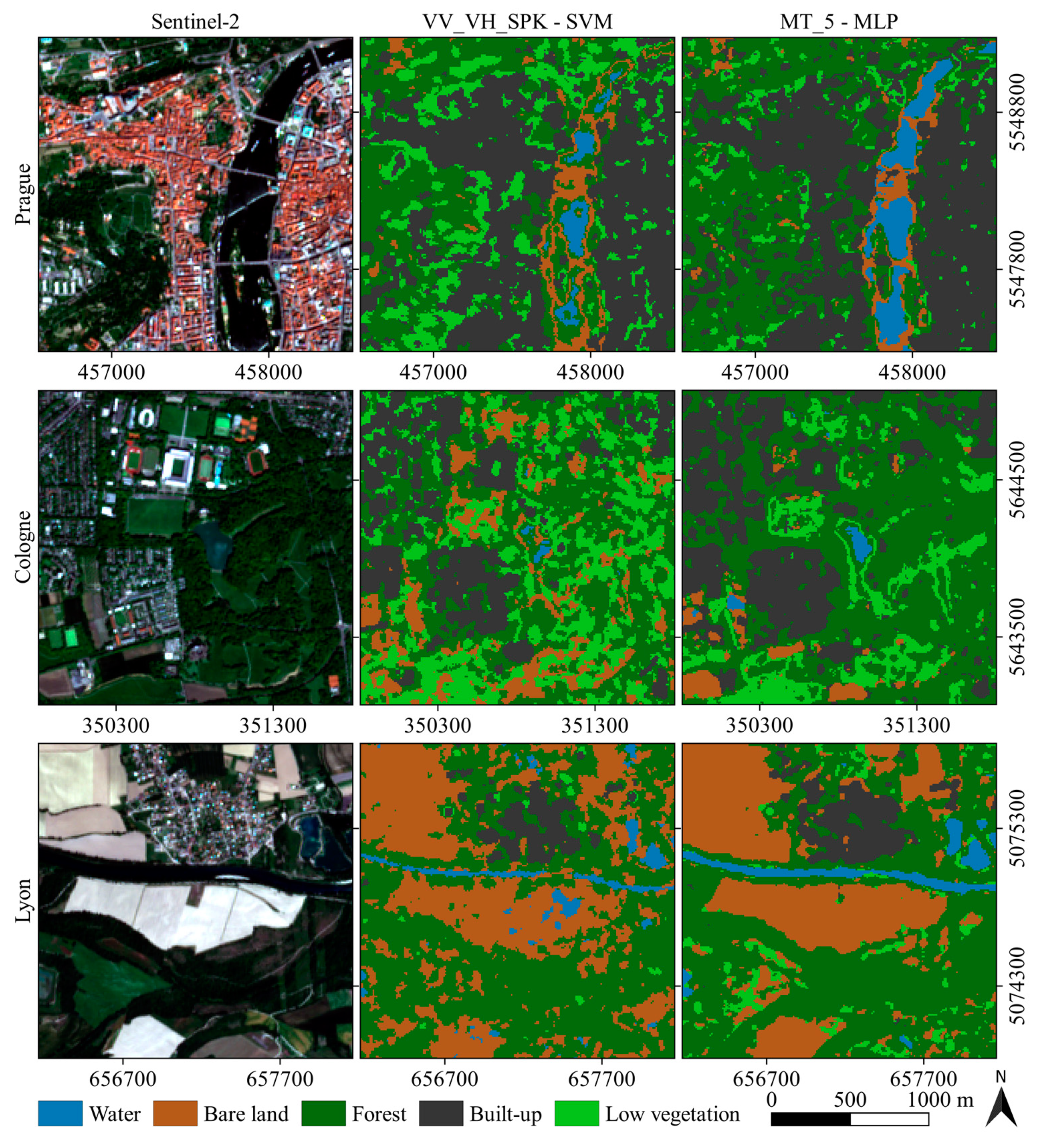
Table 1.
Multitemporal S1 imagery used in this research.
| Study Area | Date | Satellite | Acquisition Orbit |
|---|---|---|---|
| Prague | 05 May 2019 | S1B | DESC |
| 31 May 2019 | S1A | DESC | |
| 06 June 2019 | S1B | DESC | |
| 12 June 2019 | S1A | DESC | |
| 18 June 2019 | S1B | DESC | |
| Cologne | 01 May 2019 | S1A | ASC |
| 07 May 2019 | S1B | ASC | |
| 13 May 2019 | S1A | ASC | |
| 19 May 2019 | S1B | ASC | |
| 25 May 2019 | S1A | ASC | |
| Lyon | 17 May 2019 | S1B | ASC |
| 23 May 2019 | S1A | ASC | |
| 04 June 2019 | S1A | ASC | |
| 10 June 2019 | S1B | ASC | |
| 16 June 2019 | S1A | ASC |
Table 2.
The polygon samples used for training (Train) and validation (Valid).
| Prague | Cologne | Lyon | ||||
|---|---|---|---|---|---|---|
| Class | Train | Valid | Train | Valid | Train | Valid |
| Water | 105 | 45 | 105 | 45 | 105 | 45 |
| Bare land | 140 | 60 | 140 | 60 | 140 | 60 |
| Forest | 140 | 60 | 154 | 66 | 140 | 60 |
| Built-up | 140 | 60 | 140 | 60 | 140 | 60 |
| Low vegetation | 140 | 60 | 154 | 66 | 140 | 60 |
| Total | 665 | 285 | 693 | 297 | 665 | 285 |
Table 3.
The mean values of overall accuracy (OA), K, the F1 measure (F1), and the Figure of Merit (FoM) in different classification scenarios using S1 imagery with six machine learning classifiers (the bold values indicate the most accurate performance achieved for each classification scenario).
Table 3.
The mean values of overall accuracy (OA), K, the F1 measure (F1), and the Figure of Merit (FoM) in different classification scenarios using S1 imagery with six machine learning classifiers (the bold values indicate the most accurate performance achieved for each classification scenario).
| Method | OA | K | Water | Bare Land | Forest | Built-Up | Low Veg. | ||||||
|---|---|---|---|---|---|---|---|---|---|---|---|---|---|
| F1 | FoM | F1 | FoM | F1 | FoM | F1 | FoM | F1 | FoM | ||||
| VV_VH | RF | 55.37 | 0.42 | 0.52 | 0.42 | 0.57 | 0.41 | 0.49 | 0.36 | 0.46 | 0.35 | 0.58 | 0.41 |
| XGB | 57.26 | 0.44 | 0.53 | 0.43 | 0.59 | 0.43 | 0.49 | 0.38 | 0.50 | 0.37 | 0.61 | 0.44 | |
| MLP | 57.05 | 0.44 | 0.53 | 0.41 | 0.59 | 0.44 | 0.40 | 0.37 | 0.53 | 0.39 | 0.65 | 0.48 | |
| SVM | 61.63 | 0.49 | 0.55 | 0.47 | 0.61 | 0.47 | 0.52 | 0.42 | 0.58 | 0.43 | 0.68 | 0.51 | |
| AB | 60.20 | 0.48 | 0.55 | 0.45 | 0.60 | 0.46 | 0.51 | 0.40 | 0.56 | 0.41 | 0.67 | 0.50 | |
| ELM | 52.11 | 0.38 | 0.50 | 0.39 | 0.56 | 0.39 | 0.44 | 0.33 | 0.34 | 0.29 | 0.57 | 0.39 | |
| VV_VH_SPK | RF | 75.78 | 0.67 | 0.61 | 0.58 | 0.77 | 0.63 | 0.75 | 0.61 | 0.72 | 0.58 | 0.77 | 0.64 |
| XGB | 76.07 | 0.68 | 0.61 | 0.57 | 0.77 | 0.63 | 0.75 | 0.61 | 0.74 | 0.60 | 0.78 | 0.64 | |
| MLP | 76.48 | 0.67 | 0.59 | 0.57 | 0.74 | 0.61 | 0.76 | 0.62 | 0.78 | 0.64 | 0.79 | 0.65 | |
| SVM | 80.24 | 0.73 | 0.65 | 0.61 | 0.81 | 0.68 | 0.79 | 0.66 | 0.80 | 0.68 | 0.83 | 0.71 | |
| AB | 78.10 | 0.70 | 0.63 | 0.61 | 0.80 | 0.67 | 0.77 | 0.63 | 0.78 | 0.64 | 0.81 | 0.68 | |
| ELM | 72.79 | 0.63 | 0.59 | 0.54 | 0.76 | 0.61 | 0.71 | 0.57 | 0.59 | 0.48 | 0.75 | 0.61 | |
| MT_3 | RF | 88.62 | 0.84 | 0.80 | 0.77 | 0.92 | 0.85 | 0.88 | 0.79 | 0.76 | 0.66 | 0.89 | 0.80 |
| XGB | 87.96 | 0.83 | 0.79 | 0.77 | 0.92 | 0.85 | 0.87 | 0.78 | 0.75 | 0.64 | 0.88 | 0.79 | |
| MLP | 92.27 | 0.89 | 0.90 | 0.85 | 0.93 | 0.88 | 0.92 | 0.85 | 0.81 | 0.72 | 0.91 | 0.84 | |
| SVM | 90.14 | 0.86 | 0.80 | 0.78 | 0.93 | 0.87 | 0.90 | 0.82 | 0.80 | 0.70 | 0.90 | 0.83 | |
| AB | 81.58 | 0.75 | 0.76 | 0.72 | 0.88 | 0.77 | 0.79 | 0.67 | 0.66 | 0.55 | 0.80 | 0.69 | |
| ELM | 70.42 | 0.60 | 0.69 | 0.63 | 0.79 | 0.64 | 0.66 | 0.52 | 0.40 | 0.37 | 0.70 | 0.56 | |
| MT_5 | RF | 92.26 | 0.89 | 0.91 | 0.86 | 0.93 | 0.88 | 0.92 | 0.85 | 0.81 | 0.71 | 0.93 | 0.86 |
| XGB | 91.73 | 0.89 | 0.91 | 0.85 | 0.93 | 0.87 | 0.92 | 0.85 | 0.80 | 0.70 | 0.92 | 0.85 | |
| MLP | 93.95 | 0.92 | 0.92 | 0.87 | 0.95 | 0.91 | 0.93 | 0.88 | 0.86 | 0.77 | 0.93 | 0.88 | |
| SVM | 92.92 | 0.90 | 0.89 | 0.82 | 0.94 | 0.88 | 0.92 | 0.85 | 0.80 | 0.70 | 0.92 | 0.85 | |
| AB | 91.55 | 0.88 | 0.89 | 0.84 | 0.93 | 0.88 | 0.91 | 0.84 | 0.79 | 0.69 | 0.92 | 0.85 | |
| ELM | 79.02 | 0.71 | 0.80 | 0.71 | 0.84 | 0.72 | 0.77 | 0.64 | 0.47 | 0.44 | 0.79 | 0.65 | |
Table 4.
The mean values of user’s accuracy (UA) and producer’s accuracy (PA) of individual land-cover (LC) classes in different classification scenarios using S1 imagery (the best UA and PA values for scenario are highlighted in bold).
Table 4.
The mean values of user’s accuracy (UA) and producer’s accuracy (PA) of individual land-cover (LC) classes in different classification scenarios using S1 imagery (the best UA and PA values for scenario are highlighted in bold).
| Method | Water | Bare land | Forest | Built-Up | Low Veg. | ||||||
|---|---|---|---|---|---|---|---|---|---|---|---|
| UA | PA | UA | PA | UA | PA | UA | PA | UA | PA | ||
| VV_VH | RF | 47.43 | 66.49 | 50.70 | 66.44 | 63.44 | 39.91 | 37.63 | 59.80 | 58.22 | 59.93 |
| XGB | 48.26 | 67.60 | 51.06 | 70.22 | 65.01 | 40.05 | 44.10 | 57.88 | 59.77 | 64.29 | |
| MLP | 48.95 | 60.94 | 47.93 | 79.57 | 72.80 | 28.02 | 53.95 | 57.32 | 58.77 | 75.55 | |
| SVM | 49.54 | 70.88 | 52.49 | 76.75 | 71.12 | 42.00 | 61.73 | 55.13 | 64.39 | 74.53 | |
| AB | 48.38 | 70.54 | 51.01 | 75.84 | 69.10 | 40.98 | 57.58 | 54.74 | 64.20 | 72.02 | |
| ELM | 46.03 | 63.93 | 49.05 | 67.33 | 58.50 | 36.04 | 31.53 | 38.12 | 55.58 | 60.88 | |
| VV_VH_SPK | RF | 59.71 | 73.50 | 73.94 | 80.72 | 81.56 | 69.34 | 69.09 | 76.68 | 75.86 | 79.86 |
| XGB | 59.23 | 72.99 | 74.27 | 80.91 | 81.91 | 69.64 | 71.95 | 76.48 | 75.65 | 80.85 | |
| MLP | 75.02 | 58.21 | 67.27 | 81.62 | 82.17 | 70.13 | 81.75 | 75.17 | 79.63 | 79.06 | |
| SVM | 60.61 | 76.86 | 76.51 | 86.08 | 84.81 | 74.23 | 87.97 | 73.96 | 80.62 | 86.40 | |
| AB | 60.73 | 76.50 | 74.11 | 86.22 | 84.16 | 70.36 | 79.72 | 76.26 | 79.20 | 83.37 | |
| ELM | 53.37 | 73.66 | 71.46 | 81.70 | 80.06 | 65.06 | 66.76 | 53.23 | 71.83 | 80.44 | |
| MT_3 | RF | 76.02 | 91.36 | 90.48 | 93.09 | 89.95 | 87.12 | 72.32 | 81.62 | 89.56 | 88.05 |
| XGB | 74.90 | 91.60 | 91.21 | 92.63 | 89.68 | 85.49 | 69.64 | 81.53 | 88.90 | 87.82 | |
| MLP | 95.04 | 86.20 | 93.91 | 92.85 | 90.96 | 94.07 | 90.91 | 73.80 | 90.94 | 91.04 | |
| SVM | 76.99 | 91.49 | 93.21 | 94.39 | 90.23 | 88.78 | 79.91 | 80.47 | 90.27 | 90.97 | |
| AB | 71.43 | 89.65 | 86.14 | 89.52 | 83.23 | 75.52 | 59.03 | 74.99 | 80.30 | 80.77 | |
| ELM | 62.64 | 88.13 | 76.34 | 83.17 | 74.32 | 59.36 | 35.81 | 45.86 | 68.03 | 71.92 | |
| MT_5 | RF | 90.34 | 93.07 | 92.20 | 94.35 | 91.50 | 92.75 | 79.63 | 82.94 | 93.24 | 92.07 |
| XGB | 89.89 | 92.66 | 92.10 | 93.85 | 91.34 | 91.91 | 76.81 | 83.71 | 92.35 | 91.30 | |
| MLP | 89.26 | 95.34 | 94.54 | 96.16 | 91.83 | 94.91 | 93.16 | 79.31 | 93.72 | 93.26 | |
| SVM | 90.13 | 89.66 | 92.56 | 94.65 | 91.81 | 92.39 | 77.09 | 83.56 | 90.93 | 93.08 | |
| AB | 86.03 | 93.42 | 92.38 | 94.44 | 91.25 | 91.17 | 75.68 | 83.91 | 92.71 | 91.02 | |
| ELM | 77.07 | 87.33 | 81.53 | 87.38 | 79.31 | 75.49 | 48.84 | 48.06 | 76.36 | 80.97 | |
Table 5.
McNemar’s chi-squared values test results comparing SVM and MLP classifiers with other classification algorithms in the single-date and MT classification scenarios, respectively. If a χ2 value is less than 3.84 (bold values), the null hypothesis is not rejected, which indicates that the two classification results were not significantly different.
| Study Area | Class. Scenario | RF | XGB | MLP | SVM | AB | ELM |
|---|---|---|---|---|---|---|---|
| Prague | VV_VH | 46.74 | 20.71 | 29.90 | X | 39.49 | 116.67 |
| VV_VH_SPK | 66.21 | 56.46 | 14.52 | X | 0.10 | 71.15 | |
| MT_3 | 78.63 | 97.86 | X | 39.95 | 113.24 | 354.83 | |
| MT_5 | 23.43 | 29.17 | X | 3.92 | 31.17 | 226.17 | |
| Cologne | VV_VH | 12.98 | 13.85 | 15.15 | X | 0.48 | 31.17 |
| VV_VH_SPK | 9.03 | 6.25 | 24.85 | X | 0.00 | 76.59 | |
| MT_3 | 17.60 | 18.71 | X | 7.36 | 21.19 | 207.76 | |
| MT_5 | 9.22 | 12.20 | X | 6.37 | 11.84 | 208.71 | |
| Lyon | VV_VH | 31.73 | 16.62 | 25.28 | X | 1.78 | 44.21 |
| VV_VH_SPK | 19.38 | 22.26 | 5.89 | X | 6.47 | 27.76 | |
| MT_3 | 4.29 | 7.93 | X | 0.27 | 10.54 | 121.95 | |
| MT_5 | 0.06 | 1.93 | X | 1.84 | 3.67 | 128.72 |
© 2020 by the authors. Licensee MDPI, Basel, Switzerland. This article is an open access article distributed under the terms and conditions of the Creative Commons Attribution (CC BY) license (http://creativecommons.org/licenses/by/4.0/).
Share and Cite
MDPI and ACS Style
Gašparović, M.; Dobrinić, D. Comparative Assessment of Machine Learning Methods for Urban Vegetation Mapping Using Multitemporal Sentinel-1 Imagery. Remote Sens. 2020, 12, 1952. https://doi.org/10.3390/rs12121952
AMA Style
Gašparović M, Dobrinić D. Comparative Assessment of Machine Learning Methods for Urban Vegetation Mapping Using Multitemporal Sentinel-1 Imagery. Remote Sensing. 2020; 12(12):1952. https://doi.org/10.3390/rs12121952
Chicago/Turabian StyleGašparović, Mateo, and Dino Dobrinić. 2020. "Comparative Assessment of Machine Learning Methods for Urban Vegetation Mapping Using Multitemporal Sentinel-1 Imagery" Remote Sensing 12, no. 12: 1952. https://doi.org/10.3390/rs12121952
Note that from the first issue of 2016, this journal uses article numbers instead of page numbers. See further details here.