A Coarse-to-Fine Deep Learning Based Land Use Change Detection Method for High-Resolution Remote Sensing Images
by
 ,
,
Mingchang Wang
1,2 ,
,
Haiming Zhang
1,*,
Weiwei Sun
3,
Sheng Li
2,4,
Fengyan Wang
1 and
Guodong Yang
1 1
College of Geo-Exploration Science and Technology, Jilin University, Changchun 130026, China
2
Key Laboratory of Urban Land Resources Monitoring and Simulation, MNR, Shenzhen 518000, China
3
Department of Geography and Spatial Information Techniques, Ningbo University, Ningbo 315211, China
4
Shenzhen Municipal Planning & Land Real Estate Information Centre, Shenzhen 518034, China
*
Author to whom correspondence should be addressed.
Remote Sens. 2020, 12(12), 1933; https://doi.org/10.3390/rs12121933
Submission received: 29 April 2020
/
Revised: 12 June 2020
/
Accepted: 13 June 2020
/
Published: 15 June 2020
(This article belongs to the Special Issue Recent Advances in Land Cover Classification and Change Detection in 2D and 3D)
Abstract
:In recent decades, high-resolution (HR) remote sensing images have shown considerable potential for providing detailed information for change detection. The traditional change detection methods based on HR remote sensing images mostly only detect a single land type or only the change range, and cannot simultaneously detect the change of all object types and pixel-level range changes in the area. To overcome this difficulty, we propose a new coarse-to-fine deep learning-based land-use change detection method. We independently created a new scene classification dataset called NS-55, and innovatively considered the adaptation relationship between the convolutional neural network (CNN) and the scene complexity by selecting the CNN that best fit the scene complexity. The CNN trained by NS-55 was used to detect the category of the scene, define the final category of the scene according to the majority voting method, and obtain the changed scene by comparison to obtain the so-called coarse change result. Then, we created a multi-scale threshold (MST) method, which is a new method for obtaining high-quality training samples. We used the high-quality samples selected by MST to train the deep belief network to obtain the pixel-level range change detection results. By mapping coarse scene changes to range changes, we could obtain fine multi-type land-use change detection results. Experiments were conducted on the Multi-temporal Scene Wuhan dataset and aerial images of a particular area of Dapeng New District, Shenzhen, where promising results were achieved by the proposed method. This demonstrates that the proposed method is practical, easy-to-implement, and the NS-55 dataset is physically justified. The proposed method has the potential to be applied in the large scale land use fine change detection problem and qualitative and quantitative research on land use/cover change based on HR remote sensing data.
1. Introduction
Change detection is the process of comparing objects, scenes, or phenomena in different time dimensions to identify their state differences [1,2]. Remote sensing image change detection is a multidisciplinary interdisciplinary technology involving geosciences, statistics, and computer science [2]. With the development of various optical satellite sensors capable of acquiring high-resolution (HR) images, related research on the use of HR images for land cover has become popular in the field of remote sensing. In these studies, remote sensing image change detection uses images from different periods covering the same geographic area to study changes in the Earth’s surface over a period of time, which has proven to be a practical technique [3,4,5]. It uses remote sensing images and related geographic data from different periods, combined with the remote sensing imaging principle and ground characteristics. At the same time, it uses images, graphic theory, and mathematical models to determine and analyze the range and type of land cover changes. It is widely and in-depth used in land planning, urban change, disaster monitoring, military, agriculture and forestry, and other global land cover change studies. Land cover change is the result of the combined effects of natural processes and human activities and is a core issue in the study of global change [6,7].
HR remote sensing images can provide more detailed land cover information. They can make detailed comparisons of geographical objects in different periods, greatly expanding the application range of remote sensing image change detection [8,9]. Recently, HR remote sensing images have become the main data sources for change detection research. Although the fine contextual information and complex spatial characteristics that HR images convey offer rich spatial details for land cover analysis, some new challenges have emerged: intra-class variabilities are enhanced, spectral features of different objects are confused with each other; more intraclass variability leads to lower class separability and thus more confusion between classes, and the difficulty of extracting information is also increased. As far as HR remote sensing image change detection is concerned, the technologies suitable for automatic interpretation and information extraction of HR remote sensing images are relatively scarce, and the application of related technologies has not reached the stage of practical application [10].
Among the many existing change detection technologies, the most common and easy to apply is unsupervised pixel-based change detection. These traditional methods are based on directly comparing the pixels on the images of different periods to determine whether the object has changed so as to obtain information about the change of land cover. Change vector analysis, image difference, image ratio, and a binary threshold are relatively classic methods [11,12,13,14]. Due to unpredictable high-frequency components, geometric registration errors and imperfect radiation correction in HR remote sensing images, the performance of the traditional method based on pixels may be reduced and cannot be hard to apply to HR remote sensing images. This is because these methods neglect the spatial context information of the image and use a single-pixel as its basic unit [15,16,17,18]. The object-based change detection method compares the spectral features, geometric features, or semantic features extracted from the object by adding information such as texture and space, and uses the object instead of the pixel as the unit for detecting change, thereby reducing boundary effects and image registration problems. However, most of these methods are rough detection, that is, only one type of object or only the change range of the object is detected. For example, some of these methods only detect a specific category (such as buildings), and some only detect changes in the location of all objects in the study area. The detection accuracy may be very high, but there are limitations [19,20,21].
The advancement and development of machine learning have made it possible to extract the deep features of ground objects automatically [22,23]. Deep learning [24,25], as an important branch of machine learning, can automatically combine simple features into complex features and use complex features to learn the inner law of the sample data. Since AlexNet, the champion network for the ImageNet competition in 2012, was proposed, various networks with more reasonable structures and better performances have been proposed every year such as Visual Geometry Group (VGG) [26], GoogLeNet [27], Fully Convolutional Networks (FCN) [28], U-Net [29], Residual Network (ResNet) [30], Squeeze-and-Excitation Networks (SENet) [31], etc. In the field of remote sensing image processing, many deep learning methods for image classification, target detection, and change detection have been derived based on these networks. Convolutional neural networks (CNN) have been successfully applied in image classification, and many improved CNNs with excellent performance have emerged [32,33,34,35]. These CNNs are also widely used in the field of change detection, and their applicability is also very robust. However, in terms of change detection, it is difficult to detect multiple types of objects based on deep learning methods, since the methods either detect a specific category or simply identify changed locations [36,37]. Whether it is designing a better network or adding some new algorithms on the basis of CNN, almost no comprehensive detection of multiple types of objects has been achieved. Some authors have tried to realize the detection of multiple objects by adding indexes such as the normalized difference vegetation index, normalized difference water index, morphological building index, enhanced vegetation index, etc. through the relevant algorithm to the detection process of change detection, but the categories they can detect are few (often not exceeding five categories) [38,39]. Others have used segmentation networks like FCN, U-Net, and Deeplabv3+ to achieve pixel-level change detection. Although their detection accuracy is very high, most of them only extract the change information of the building [37,40].
In the study of global environmental change, the description, quantification, and monitoring of land use/cover are particularly important [41], and land cover change has serious implications for the environment [42]. According to the detection results of the types and locations of land cover changes, global issues such as urban environmental changes and ecological changes can be better understood. In related research, it was found that few people have been able to obtain the fine change detection results of multiple types of land cover.
In order to obtain fine change detection results and extract information on various types of change objects and change positions in the study area, we propose a land-use change detection method for HR remote sensing images based on coarse to fine deep learning. The basic idea of the method in this paper was to use CNN, which is very suitable for the complexity of the scene, to classify the scene according to the result of classification to obtain the changed and unchanged scenes, depending on the scene change information to obtain the category-level coarse change detection result. Depending on the changing scene, we used a multi-scale threshold (MST) method to obtain high-quality changed and unchanged training samples by dividing the spectrum and texture change intensity values. Using these changed and unchanged samples as the training samples to train the deep belief network (DBN), a DBN can then detect the image and obtain pixel-level range detection results. By mapping the category detection results to the range detection results, a fine change detection result can be obtained. The main idea and contribution of this paper can be summarized from three aspects:
(1) The new idea of detecting a land use/cover change from coarse to fine based on deep learning is proposed, which solves the problem that the traditional method detects a single type of object or only detects the change range. The coarse detection results provide type conversion information for all objects in the study area. The pixel-level range change detection results can reflect the precise position of the object change. Mapping the coarse detection to the range changed to obtain the result of fine change detection, which can reflect the change of the type of the object at the precise position.
(2) We independently designed a new scene classification dataset, NS-55, which enriches the data sources of the remote sensing image scene classification research field and contributes to the development of related fields. When selecting CNN for scene classification, the adaptive relationship between CNN and scene complexity was innovatively considered, giving full play to the performance of CNN and improving the accuracy of scene category detection.
(3) We created a new method called MST for selecting high-quality training samples. We used MST to divide the spectral and textural change intensity value to obtain high-quality training samples. Moreover, we provide a new method for selecting training samples for the field of remote sensing image processing using deep learning, which can improve the efficiency of labelling samples and reduce the tedious work of manually labelling samples.
2. Methodology
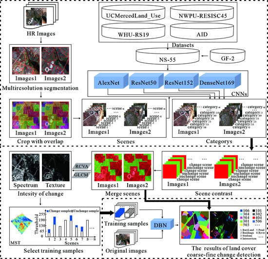
The structure diagram of the method proposed in this paper is shown in Figure 1. The method consisted of three parts. The first part was to train the CNN and detect scene categories. We used the NS-55 dataset to train the four networks of AlexNet, ResNet50, ResNet152, and DenseNet169, and we used these four CNNs to detect the category of the scene. The majority category was used to obtain the final category of the scene, and the scene category was compared to obtain the changed scene. In this part, the coarse change detection result was obtained. The second part was to use MST to extract the training samples. Robust change vector analysis (RCVA) and gray-level co-occurrence matrix (GLCM) algorithms were used to extract the intensity values of the image spectrum and texture changes. In different scenarios, MST was used to divide the change intensity values to separate the changed samples from the unchanged samples. In this part, high-quality training samples could be obtained. The third part was to train the DBN with samples and detect pixel-level range changes. The category detection results were mapped to the range detection results to obtain fine change detection results. We conducted experiments based on the Multi-temporal Scene Wuhan dataset and aerial images of a particular area of Dapeng New District, Shenzhen to verify the feasibility of our method.
2.1. NS-55 Dataset
In addition to the impact of preprocessing results and CNNs on the detection results of deep learning change detection based on scene classification, the datasets used for training often determine the richness of its detection categories, which in turn affects the accuracy of the detection results. In order to obtain a dataset containing more scene categories than the general dataset, we produced an NS-55 scene classification dataset. The data in NS-55 came from NWPU-RESISC45 [43], UCMercedLand_Use [44], WHU-RS19 [45], and AID [46], and added a large number of scene images cropped from Gaofen-2 satellite remote sensing images.
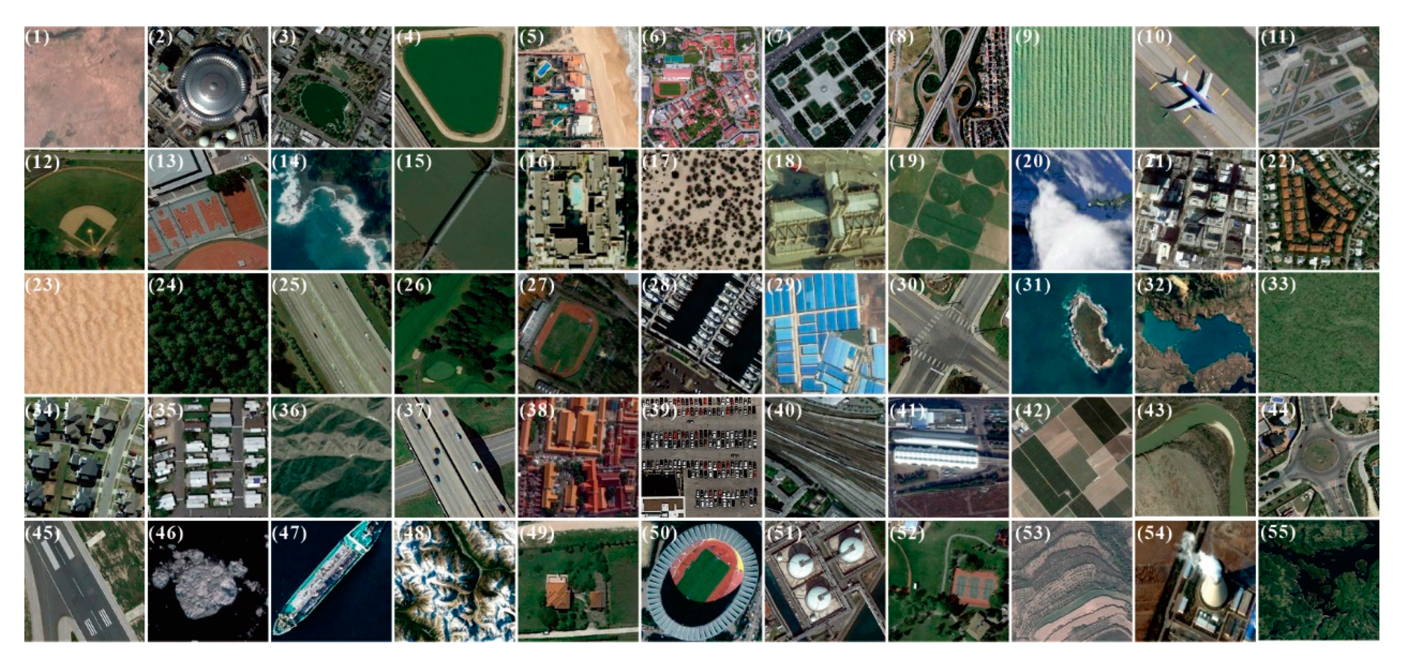
This dataset contains 55 types of remote sensing scenes: (1) bare land, (2) center, (3) park, (4) pond, (5) resort, (6) school, (7) square, (8) viaduct, (9) agricultural, (10) airplane, (11) airport, (12) baseball_diamond, (13) basketball_court, (14) beach, (15) bridge, (16) buildings, (17) chaparral, (18) church, (19) circular_farmland, (20) cloud, (21) commercial_area, (22) dense_residential, (23) desert, (24) forest, (25) freeway, (26) golf_course, (27) ground_track_field, (28) harbor, (29) industrial_area, (30) intersection, (31) island, (32) lake, (33) meadow, (34) medium_residential, (35) mobile_home_park, (36) mountain, (37) overpass, (38) palace, (39) parking_lot, (40) railway, (41) railway_station, (42) rectangular_farmland, (43) river, (44) roundabout, (45) runway, (46) sea_ice, (47) ship, (48) snowberg, (49) sparse_residential, (50) stadium, (51) storage_tank, (52) tennis_court, (53) terrace, (54) thermal_power_station, and (55) wetland. NS-55 contains 55 types of scenes, each containing 700 scene images (RGB images) with a size of 256 * 256 pixels or 600 * 600 pixels. The spatial resolution of the images is diverse and comes from more than 100 countries around the world. At the same time, the weather, light, season, angle of view, and other factors in the dataset are quite different and are more representative, as shown in Figure 2.
2.2. Coarse Deep-Learning Change Detection
With the continuous development of artificial intelligence algorithms, deep learning has become one of the most powerful tools in the field of computer vision. In particular, the widespread application of CNN in the image field and its network structure are being optimized continuously, which has further deepened and expanded the research of remote sensing image scene classification [47,48].
There is a specific adaptive relationship between the complexity of remote sensing images and the depth of CNN. That is, when using shallow and deep CNN to classify images with low complexity and high complexity, respectively, if the correspondence between CNN and image complexity is effectively used, the inherent characteristics of CNN can be fully utilized to improve classification accuracy [49]. According to Zhang Xiaonan et al. [45] and Li, H [49], AlexNet has a high recognition rate for macroscopic scenes such as snow mountain, beach, cloud, runway, forest, and bridges; ResNet50 has a high recognition rate for scenes with fixed shapes such as basketball courts, baseball fields, golf courses, ground track field, and airplanes; DenseNet169 has a higher recognition rate for abstract scenes with more semantic features such as the park, harbor, chaparral, sea ice, and island; and ResNet152 has a high recognition rate for scenes such as lakes, terraces, thermal power station, and mobile home park. AlexNet and ResNet are the champions of the classification task of the ImageNet competition in 2012 and 2015, respectively, and DenseNet is a CNN model with a better performance developed on the basis of ResNet. This paper selected the above four CNNs as the basic network for scene classification:
(1) AlexNet: AlexNet contains five convolutional layers and three fully connected layers. Using ReLU as the activation function, the problem of gradient disappearance is solved. A regularization layer was added after the first convolutional layer and the second pooling layer. It uses the maximum pooling technique for pooling, and it uses the Dropout technique after the convolutional layer to prevent overfitting [32].
(2) ResNet: ResNet solves the problem of network degradation with the deepening of the network by designing the residual module. Assuming that is the input of the th layer in the network, the output of the directly connected CNN at the l layer can be formalized as:
The design of the residual block makes the output of the layer become:
That is, the problem of network degradation is solved by adding identity mapping. Introducing the batch normalization layer after the convolutional layer and the pooling layer makes the network easier to train. ResNet includes ResNet18, ResNet34, ResNet50, ResNet101, ResNet152, a total of five kinds, and their conv1 structure is the same, and the end of the network ends with average pool, 1000-d fc, and Softmax, but their conv2_x, conv3_x, conv4_x and conv5_x are different [35].
(3) DenseNet: DenseNet expands and develops the idea of ResNet, uses batch regularization technology to accelerate convergence, control overfitting, and adds the output of the previous convolution and pooling layers to the input of several subsequent convolutional layers. The output of the layer becomes:
The convergence speed is faster than ResNet, and the test results of the ImageNet dataset have also been significantly improved [50].
The classification dimension of the above CNN was modified to 55, and the rest of the structure remained the same as the classic network. We used NS-55 to train the above CNN and tested its classification performance.
In order to obtain the segments of the ground objects in line with the actual situation and improve the efficiency of our method in the implementation process, we used a multi-scale segmentation algorithm, which is more classic but generally used and has a good segmentation effect. The multi-scale segmentation algorithm can not only make the result of feature classification more in line with the actual distribution of ground objects, but can also effectively retain the effective information of different objects in the image [51,52]. Each of the four trained CNNs will independently assign a class to each scene, and the final class is then obtained by majority voting. Comparing the categories of scenes at the same location in the two images, the change information of the scene can be determined, then the coarse change detection result can be obtained.
2.3. Use Multi-Scale Threshold (MST) to Separate the Changed Samples from the Unchanged Samples
In the change detection method based on deep learning, the selection of high-quality training samples has been a hot research issue for many experts and scholars [37]. RCVA [53,54] and GLCM [55,56] are classic algorithms for extracting image spectrum and texture features. They have a wide range of applications and excellent feature extraction capabilities.
The RCVA algorithm considers the neighborhood information of pixels and selects the pair of pixels with the smallest spectral difference for detection, which greatly eliminates the impact of registration errors. Based on the RCVA principle, by traversing all the pixel pairs of two images one by one, the spectral change intensity values of all pixel pairs can be calculated, and then the spectral information change intensity map, considering the neighborhood information, can be obtained.
GLCM is one of the most classic methods for extracting textures, and it is also a commonly used texture feature analysis method with a good extraction effect. GLCM mainly extracts textures based on the conditional probability density between the grey levels of the image. It is a special matrix that describes the relationship between the grey levels of neighboring pixels or neighboring pixels with a certain distance [57]. Taking the variance as the scalar can best reflect the differences between different ground objects [58], after obtaining the texture variance characteristics based on the two images, the texture change intensity value can be calculated by the formula, and then the change intensity map can be obtained.
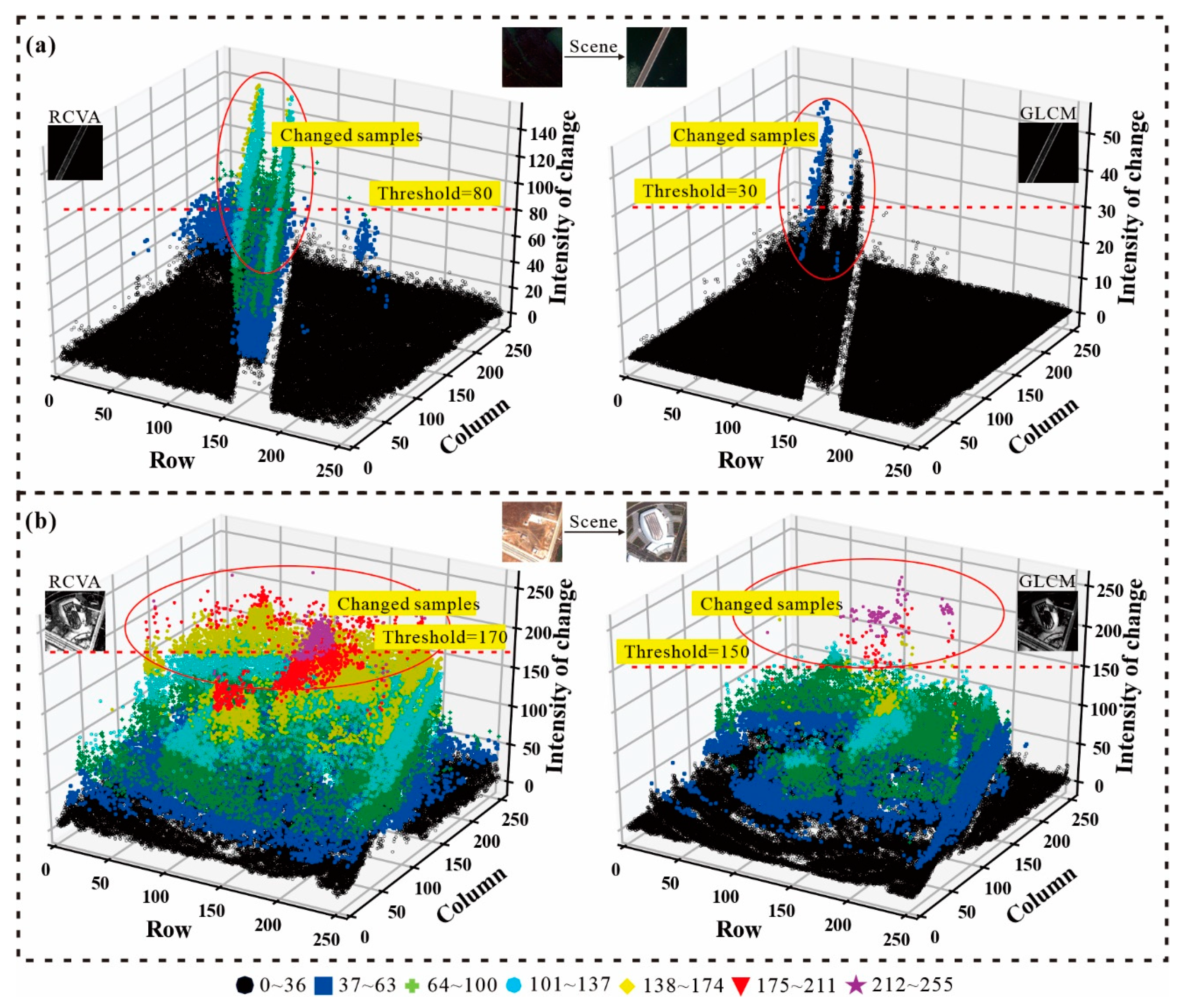
When dividing training samples according to the change intensity values of the spectrum and texture, traditional methods mostly use a certain threshold for division, and the selection of threshold has linear characteristics. This leads to a large amount of confusion between the changed samples and the unchanged samples, which dramatically reduces the quality of the samples. Based on this, we proposed a strategy for dividing samples using MST. The formula is as follows:
where represents the change intensity value of RCVA or GLCM of the th scene; is the number of pixels corresponding to the change intensity value; and is the scale coefficient.
The schematic diagram of sample division in different scenarios is shown in Figure 3.
In different scenarios (changed), different thresholds can be calculated using Equation (4). The threshold is used to divide the intensity value of the spectral and textural changes to separate the changed and unchanged samples, so as to obtain two sets of training samples corresponding to RCVA and GLCM. Finally, the combination of two sets of samples is taken as the final training sample.
2.4. Fine Deep-Learning Change Detection
Deep learning can use its own advantages to fully dig in-depth data features, which is an effective method for remote sensing big data analysis and data mining. It can cope with the challenges of complex feature information and the large amount of information brought by the improvement of remote sensing image resolution [59].
DBN [60,61] is based on the development of biological neural networks and shallow neural networks. It is a probability generation model that infers the sample data distribution by joint distribution. It uses a layer-by-layer unsupervised training method to extract features from a large number of unlabeled sample data, and optimizes the model by using a small amount of labelled sample data. Finally, it obtains the optimal weight of the network, so that the network can generate training data based on the maximum probability, forming high-level abstract features to obtain a better classification model. The DBN is mainly composed of two parts. The first part is a multi-layer restricted Boltzmann machine (RBM) [62,63] for pre-training the network. The second part is a feedforward back-propagation network, which makes the RBM stack out of the system more refined. For each RBM, there is energy as a system:
where n and m are the numbers of neurons in the explicit layer and hidden layer; and indicate the state of the neurons in the explicit layer and hidden layer; is the model parameter, where is the weight between neurons and ; and and represent the paranoia of explicit and hidden neurons, respectively.
According to the energy function, the joint probability distribution about and can be obtained, and the DBN reconstructs the sample data through the correlation calculations based on . At the same time, the input of the DBN is a vector of continuous input real-valued variables, which overcomes the shortcomings of the CNN, which must take an image of a specific size as an input. It can be easily applied to pixel-based change detection and can perform more precise detection of the picture. Using the samples selected by MST to train the DBN, a detection model with excellent performance can be obtained. By detecting the entire image, we can get the pixel-level range change detection results.
In order to evaluate the accuracy of change range detection, accuracy (), recall (), false alarm (), and missing alarm () were introduced to evaluate the detection results, as shown in Table 1. The formula is as follows:
where represents the number of positive examples; represents the number of negative examples; represents the number of positive examples correctly judged as positive examples; represents the number of positive examples incorrectly judged as negative examples; represents the number of negative examples correctly judged as negative examples; and represents the number of negative examples incorrectly judged as positive examples.
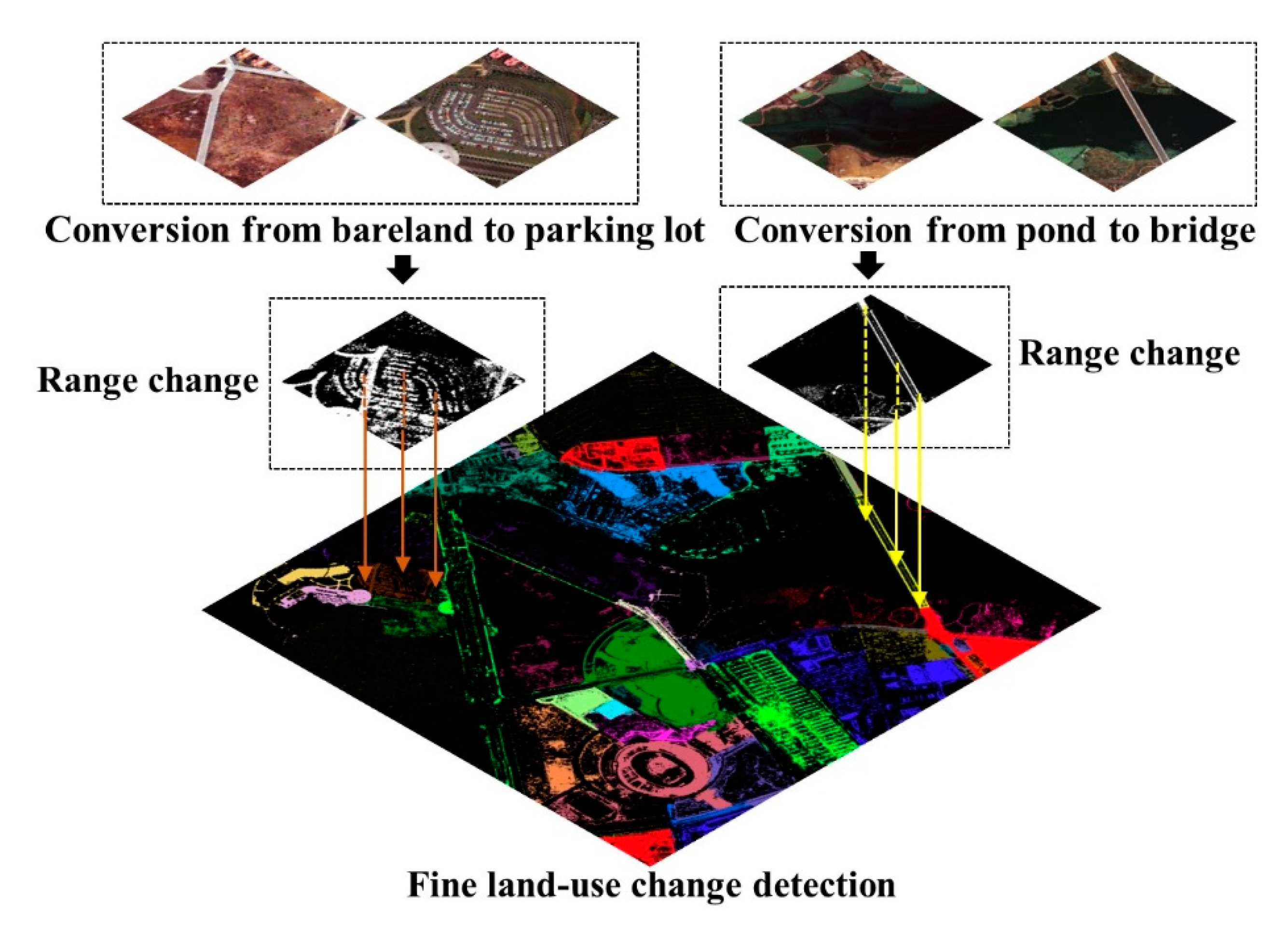
According to the principle of the change matrix, we can obtain the change trajectory of the scene, that is, from what to what. Finally, we mapped the category changes to the range changes to obtain the fine change detection results, as shown in Figure 4.
3. Experiments and Results
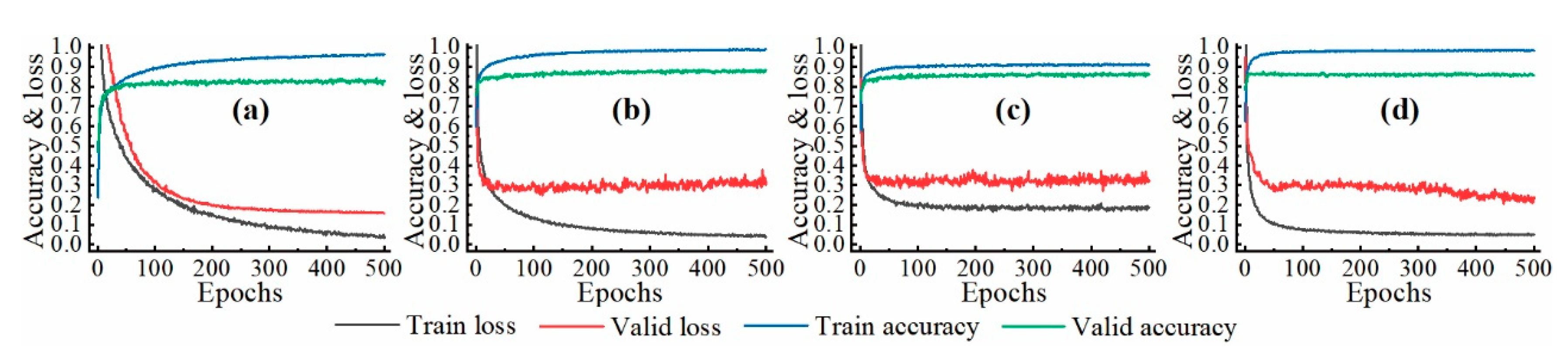
We used the NS-55 dataset to train the CNN. To accelerate the model convergence speed and improve the accuracy of model training, combined with the idea of transfer learning [64,65,66], the AlexNet, ResNet50, ResNet152, and DenseNet169 used in this paper were pre-trained models (models from torchvision), that is, a network pre-trained on the ImageNet dataset of 1000 classes. The weights of CNNs were updated after the training process, 300 images of each category were selected as the training set (a total of 16,500 (55 × 300) images), and 100 images of each category were used as the validation set (a total of 5500 (55 × 100) images). The training loss, validation loss, training accuracy, and validation accuracy of each CNN are shown in Figure 5.
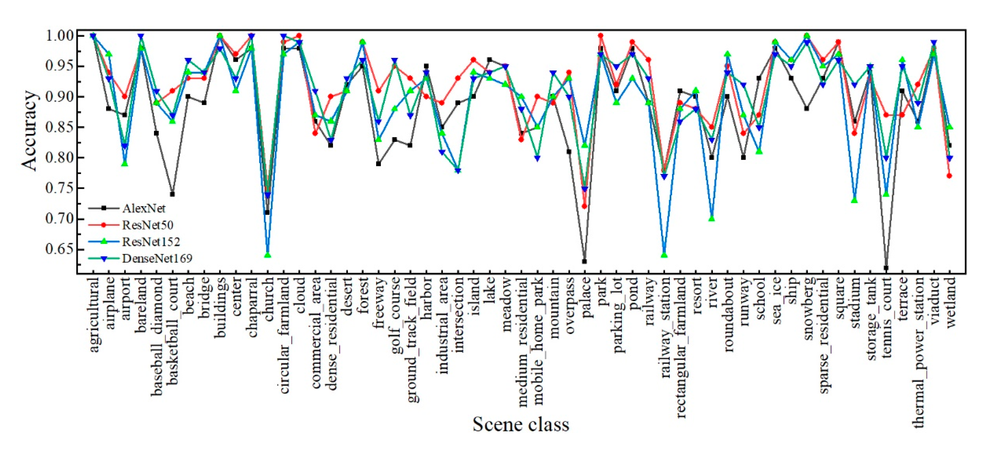
It can be seen from Figure 5 that the pre-trained CNNs had a fast convergence speed. After training within 100 epochs, the training accuracy and validation accuracy reached 80% or more. After 200 epochs or more training, the training accuracy reached 90% or more. Only the validation accuracy of AlexNet was 82%, the remaining CNNs reached 85% or higher. Training and validation loss values dropped below 0.3. We selected 300 images of each category as the test dataset (a total of 16,500 (55 × 300) images) to verify the classification accuracy of the CNN, as shown in Figure 6.
From the test results, the average test accuracy of AlexNet, ResNet50, ResNet152, and DenseNet169 were: 88.56%, 91.78%, 89.51%, and 90.85%. CNNs trained on the NS-55 dataset have better detection capabilities for various scenarios. Except for a few categories with lower test accuracy, the test accuracy for most categories was higher than 85% or even 95%, and a few reached 100%, indicating that the NS-55 dataset is reasonably designed to be suitable for CNN training, and can be used as a scene classification dataset. At the same time, CNNs have high training accuracy and can be used for scene category detection. It can also be seen that AlexNet had a high test accuracy for macro scenes such as snow mountain and beach, ResNet50 had high test accuracy for fixed-shape scenes such as basketball courts and baseball fields, DenseNet169 had high test accuracy for scenes with rich semantic features such as parks and harbors, and ResNet152 had a higher test accuracy for more complex scenes such as lakes and terraces, which further validates the adaptive relationship between the complexity of remote sensing images and the depth of the CNN.
3.1. Experiment I
3.1.1. Study Area and Data
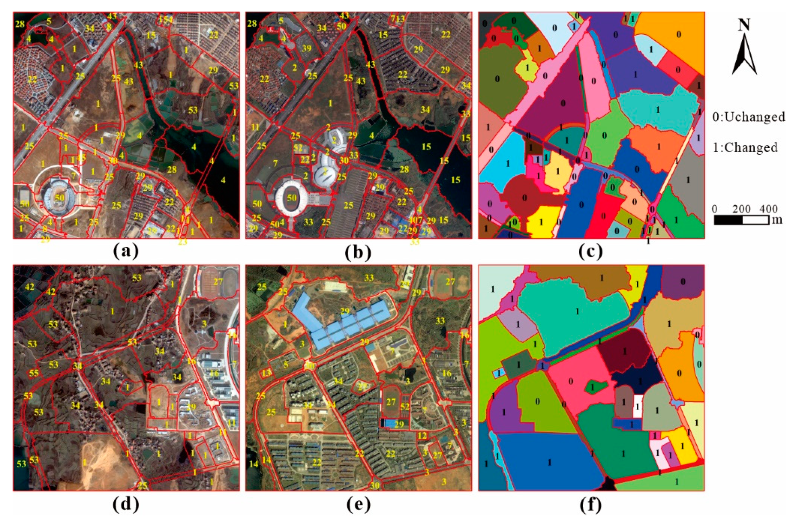
The MtS-WH dataset was published by Wuhan University’s Sensing Intelligence and Machine Learning Group, on 26 March 2019. It is mainly used for theoretical research and verification of scene change detection methods. This dataset includes two HR remote sensing images with a size of 7200 6000 pixels, obtained by IKONOS sensors, covering the Hanyang District of Wuhan, China. The images were acquired on 11 February 2002, and 24 June 2009, and were fused by the Gale–Shapley algorithm with a resolution of 1 m including four bands of red, green, blue and near-infrared, where we used only three bands of red, green, and blue. As shown in Figure 7, in this paper, two regions with multiple land categories were selected as the experimental areas (Site1 and Site2).
3.1.2. Data Processing and Accuracy Assessment
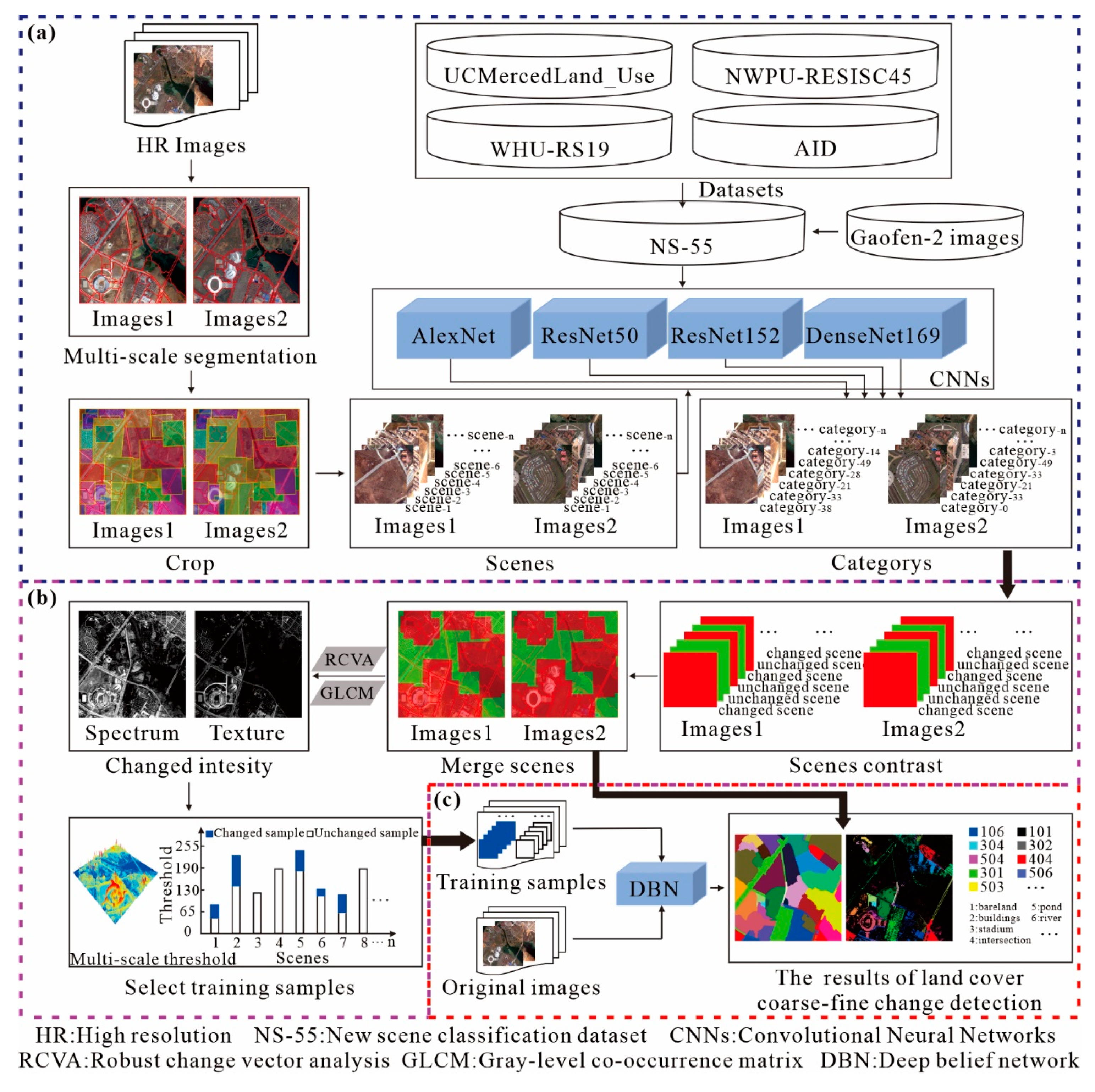
Based on the multi-scale segmentation algorithm, 73 scenes were cropped in Site1, and 44 scenes were cropped in Site2. The trained CNNs detected the categories of these scenes, and each CNN obtained a category result it detected. The final category detection result of each scene was obtained through the majority voting method, and the category change detection result (coarse change detection result) was obtained by comparing the scene categories. The category labelling numbers corresponded to the categories in the NS-55 dataset, and binary labelling was used to indicate changing and unchanging scenes, where 0 represents the unchanged scene, and 1 represents the changed scene, as shown in Figure 8.
Based on the category labels of the MtS-WH dataset (Figure 7c,d), we evaluated the classification accuracy of CNNs for the scenes in Site1 and Site2. We counted the number of changed scenes in Site1 and Site2: Site1 contained a total of 37 changed scenes and 36 unchanged scenes; Site2 contained a total of 36 changed scenes and eight unchanged scenes. The results of CNN detection were that Site1 contained a total of 39 changed scenes (four false detections) and 34 unchanged scenes (two false detections), and Site2 contained a total of 37 changed scenes (two false detections) and seven unchanged scenes (one wrong detection).
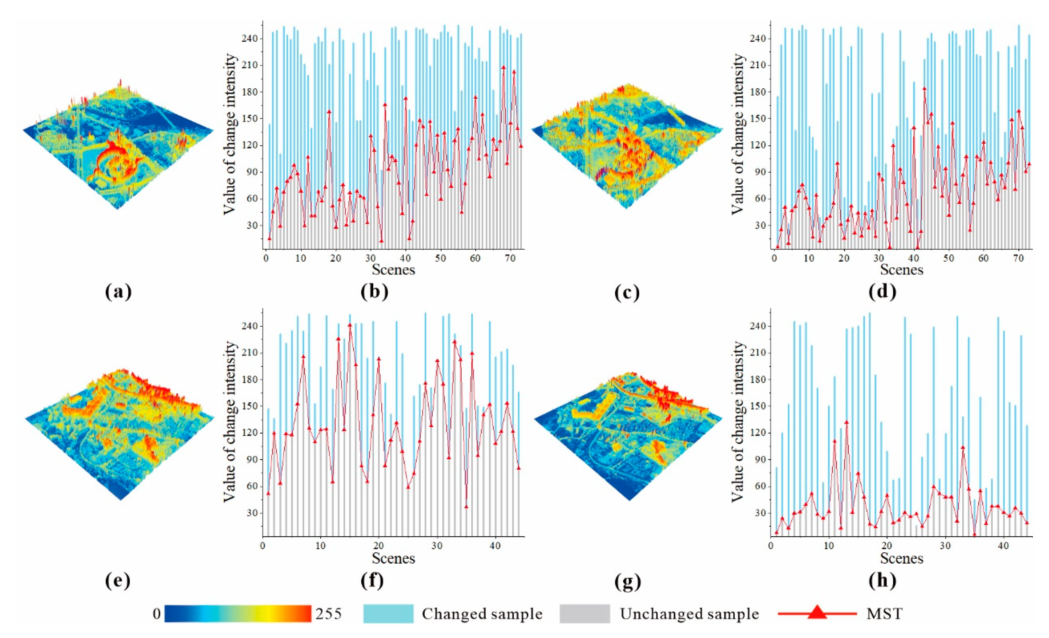
We determined the value of k as 0.8, which was used to separate the changed segments in the changed scene. At the same time, in order to ensure that the unchanged samples were distributed in the entire image, we also selected a part of the unchanged samples in the unchanged scene. Using the spectral change intensity value and the textural change intensity value, two sets of samples could be obtained, and the changed samples and the unchanged samples of the two sets of samples were respectively combined to obtain the final training samples. Schematic diagram of the sample division of Site1 and Site2, as shown in Figure 9.
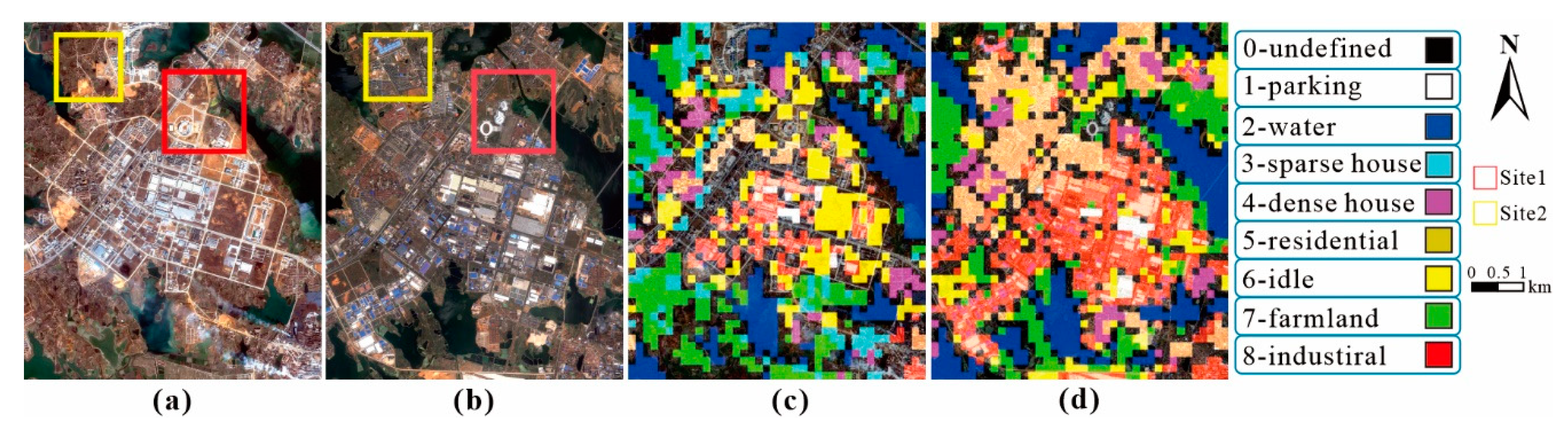
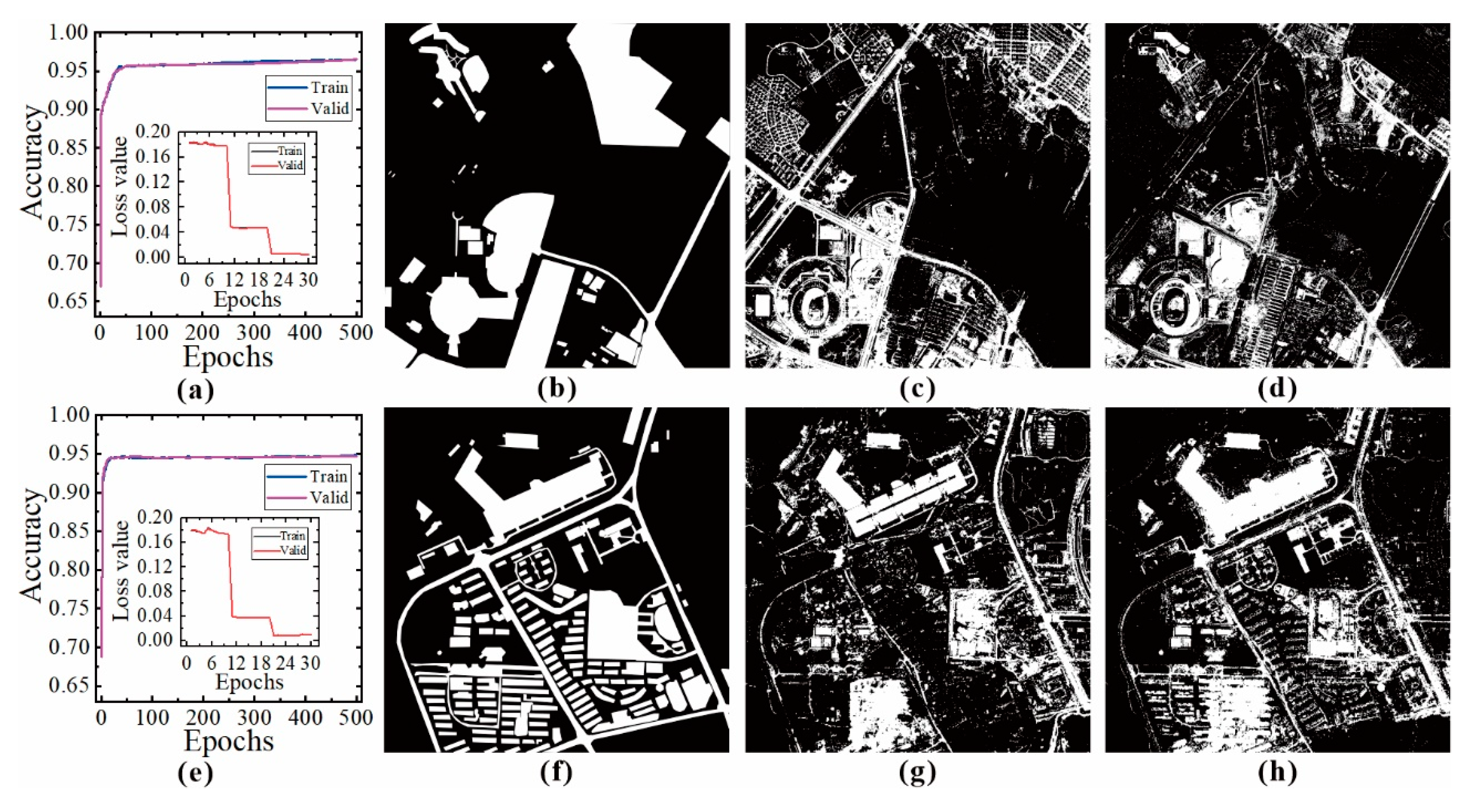
MST categorized 110,723 changed samples and 324,675 unchanged samples at Site1 and 231,972 changed samples and 1,167,469 unchanged samples at Site2. The training results of DBN and the detection results of the change range are shown in Figure 10.
We selected 8000 changed samples and 8000 unchanged samples to train the DBN. In order to compare it with the MST, 8000 training samples categorized by a single threshold were selected to train the DBN. The above range change detection results were evaluated, and the results are shown in Table 1.
From the indicators, it can be seen that the accuracy and recall of Site1 increased by more than 20%, and the false alarm rate and missing alarm decreased by more than 30%; Site2’s accuracy rate increased by more than 10%, recall rate increased by more than 35%, false alarm rate decreased by more than 10%, and missing alarm decreased by more than 35%. At the same time, the accuracy of the Site1 and Site2 detection results were more than 80%, and the recall was more than 78%.
We mapped the category change detection result to the detection result of the change range, and obtained the fine detection results of multiple types of land-use changes, as shown in Figure 11.
3.2. Experiment II
3.2.1. Study Area and Data
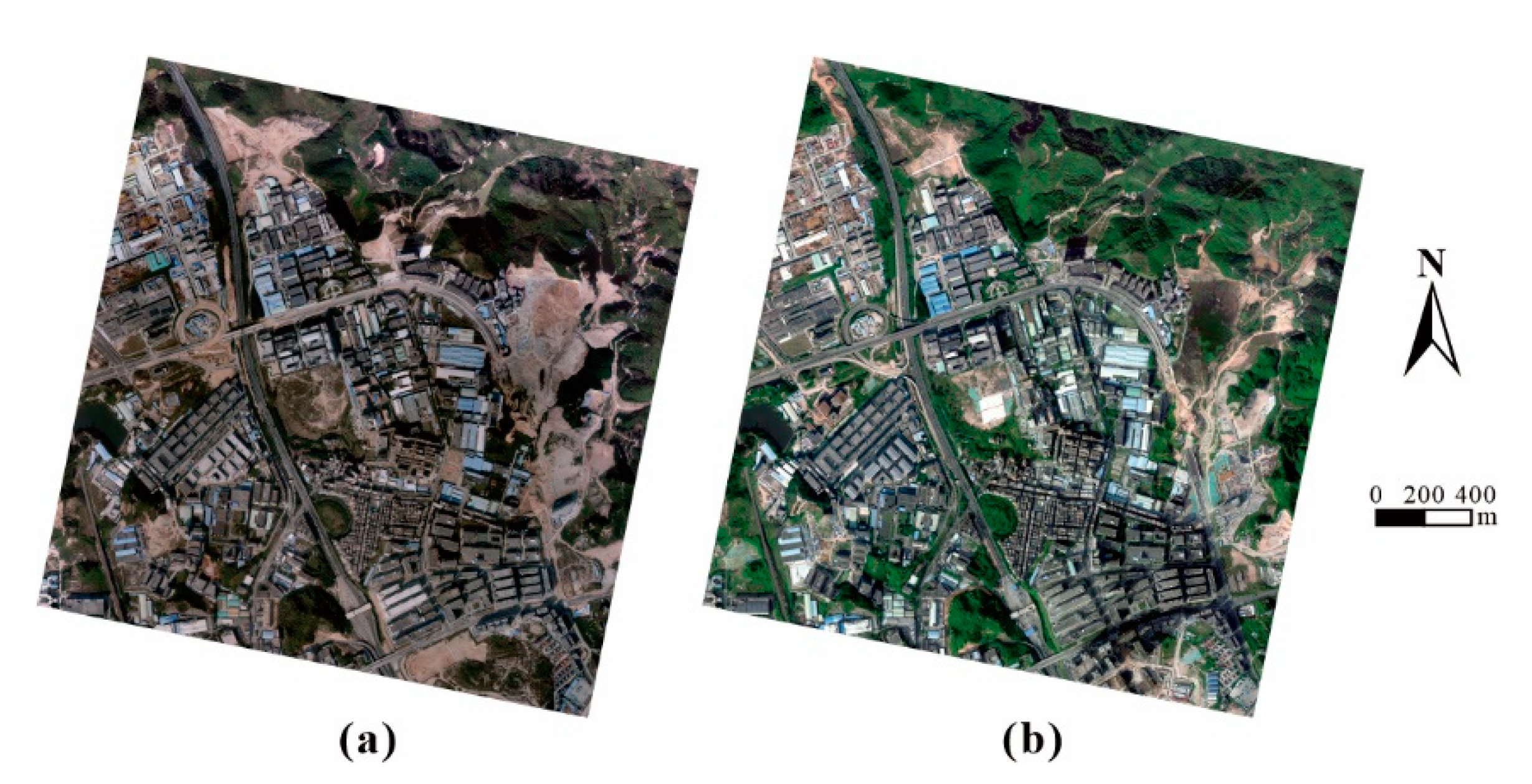
We obtained an image of an area in Dapeng New District, Shenzhen, by aerial photography. The image size was 5622 5587 pixels, the acquisition time was December 2014 and May 2017, and the resolution was 0.5 m including three bands of red, green, and blue, as shown in Figure 12.
3.2.2. Data Processing and Accuracy Assessment
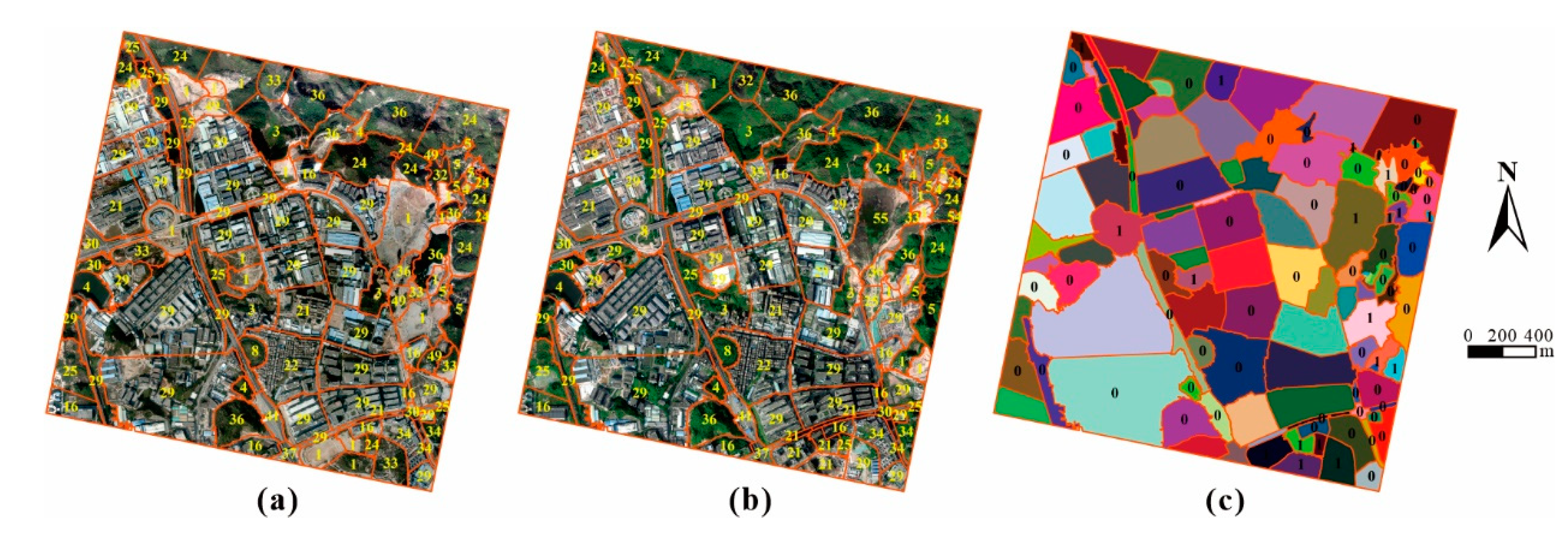
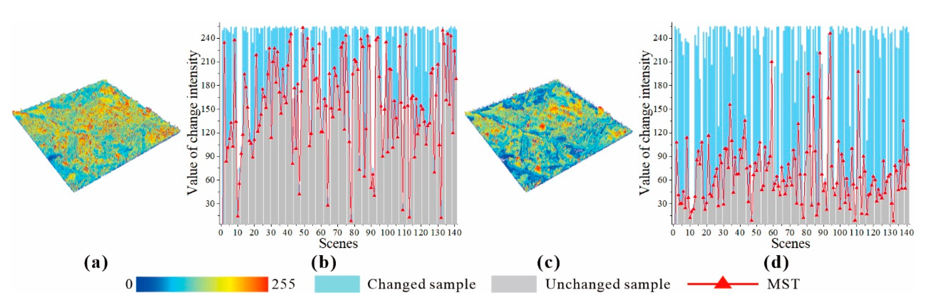
According to the data processing flow in experiment 1, segmentation, cropping, and category detection were performed on the image, and 141 scenes were cropped out. The other processing results are shown in Figure 13, Figure 14 and Figure 15.
The CNN detection results were as follows: there were 30 changed scenes (two false detections) and 111 unchanged scenes (three false detections). The index analysis of the range detection results is shown in Table 2.
From the above table, the range change detection result of this experiment had an accuracy rate of more than 91% (an increase of 5%), a recall rate of more than 77% (an increase of 47.52%), false alarm rate decreased by more than 24%, and missing alarm rate decreased by more than 47%. The fine detection results of multiple types of land-use changes are shown in Figure 16.
4. Discussion
In the field of change detection, the accuracy, meticulousness, and comprehensiveness of the change detection method reflect the level of its use-value. Whether it is pixel-based or object-based change detection, the traditional methods mostly detect a single type of land or only detect the change range (change location). Our proposed method starts with detecting the category of the scene by comparing the land cover classes of a scene at two different moments in time and using MST to select high-quality training samples and binary change value to describe change/non-change, so as to gradually obtain fine land use/cover change information. At the same time, two innovative strategies were proposed in our method (1) to improve the accuracy of CNN detection scenes; and (2) to a certain extent, solve the problem of the low quality of pixel-level training samples in the field of deep learning. The experimental results (Figure 11 and Figure 16) confirmed the superiority of our proposed method in reflecting the detailed information of land use/coverage in the study area compared with other traditional methods and obtained the effect (visual effects and description effects) that the traditional method did not.
In the research of HR remote sensing image classification tasks, training deep learning models using scene classification datasets has almost become an indispensable step. Due to the limitations of the scene classification dataset (limited categories or limited data), many people have only conducted classification in a few categories. They often choose to fix certain categories as their research object in order to explain a certain problem (the problem of forest changes, the problem of building changes, etc.). It can be observed from Figure 2 that the NS-55 dataset we designed contained a wide variety of scene categories and high-quality images, and simple and reasonable naming of categories. As can be seen from Figure 5, when we used NS-55 to train CNNs, the training accuracy and verification accuracy of each CNN could reach more than 80% accuracy in a short time (within 100 epochs). The fluctuation of the loss value was also very small and stabilized in almost 50 epochs. This means that the NS-55 we designed is fit-for-purpose: it is suitable for the network requirements of CNN and can be used in related research.
CNN trained with NS-55 had high accuracy when detecting scenes, which was verified in Figure 6. It is worth mentioning that when CNN detects scenes with complex semantic information such as churches, palaces, railway stations, and stadiums, the classification accuracy is often low. The reason may be that the semantic information in these scenes is too complicated, and the objects contained in the scene are not only the subject objects, which is also a common problem encountered when using CNN for classification. However, when we chose CNN, we innovatively considered the relationship between CNN and scene complexity, which may avoid these problems to a certain extent. As can be seen from the test accuracy of the four CNN pairs “tennis_court” in Figure 6, only the test accuracy of ResNet50 on “tennis_court” was high (above 85%), and the test accuracy of the other three networks was low (below 75%). This shows that if the adaptive relationship between CNN and scene complexity is considered when performing scene classification, the classification accuracy can be improved.
The performance of deep learning methods depends on the number and quality of training samples. Especially for models like RBM, DBM, and DBN, which use vectors with stacked spectral values of pixels as input, the confusion of positive and negative samples will lead to a reduction in the robustness of the model, and the detection ability will be greatly reduced. Figure 9 and Figure 14 proved that the quality of the training samples categorized by MST was very high, which avoids the drawback that a single threshold categorized training sample will produce much confusion. It can be concluded from Table 1 and Table 2 that the DBN trained by the training samples obtained through MST had strong detection ability and high accuracy.
Finally, we proposed mapping the category changes to the range changes, and we could obtain the fine multi-type land-use change detection results. As can be seen from Figure 10 and Figure 16, this fine land-use change detection map can more intuitively, meticulously, and accurately reflect the scope and type of land change, and can be used for land planning, urban change, disaster monitoring, military, agriculture, and forestry industry, and other fields to provide detailed information on the land change.
5. Conclusions
In this paper, a coarse-to-fine deep learning based land use change detection method for HR remote sensing images was proposed, which solved the problem of detecting only a single land type or only the range of land change and could obtain more complete change information. Our new dataset NS-55 enriched the scene classification dataset, and we used it to train the CNNs. When choosing CNNs, we innovatively considered the adaptation relationship between CNN and scene complexity. The change category obtained by CNN detection is the so-called coarse change detection result. When selecting training samples, we proposed using MST to obtain the changed and unchanged samples by dividing the intensity values of the spectrum and texture changes. This method avoids the problem of a large number of sample confusion caused by the use of a single threshold to divide the intensity value in the traditional method. MST can obtain high-quality samples, and the trained DBN can more accurately detect the change range and obtain accurate pixel-level change detection results. By mapping the category change result to the range change result, the so-called coarse to fine change detection result was obtained. Experiments were carried out on two high-resolution remote sensing image pairs. The results showed that the method has high detection accuracy and can reflect the changes in land use/cover in detail. This is a novel remote sensing image land use/cover multi-type change detection method, which has special practical value and promotion significance in the study of global issues such as urban change, land planning, disaster monitoring, and other urban environmental changes and ecological changes.
Author Contributions
Conceptualization, M.W., H.Z., and W.S.; Methodology, M.W. and H.Z.; Software, F.W.; Validation, G.Y. and H.Z.; Formal analysis, M.W., H.Z., and W.S.; Investigation, M.W. and W.S.; Resources, H.Z.; Data curation, S.L.; Writing—original draft preparation, M.W. and H.Z.; Writing—review and editing, H.Z.; Funding acquisition, M.W., G.Y., and F.W. All authors have read and agreed to the published version of the manuscript.
Funding
This research was funded by the National Natural Science Foundation of China (41472243); the Open Fund of Key Laboratory of Urban Land Resources Monitoring and Simulation, MNR (KF-2018-03-020; KF-2019-04-080); the Shanghai Institute of Geological Survey (Key Laboratory of Land Subsidence Detection and Prevention, Ministry of Land and Resources) open fund (KLLSMP201901); and the Scientific Research Project of the 13th Five-Year Plan of Jilin Province education department (JJKH20200999KJ).
Conflicts of Interest
The authors declare no conflicts of interest.
References
- Lv, P.Y.; Zhong, Y.F.; Zhao, J.; Zhang, L.P. Unsupervised Change Detection Based on Hybrid Conditional Random Field Model for High Spatial Resolution Remote Sensing Imagery. IEEE Trans. Geosci. Remote Sens. 2018, 56, 4002–4015. [Google Scholar] [CrossRef]
- Lunetta, R.S.; Johnson, D.M.; Lyon, J.G.; Crotwell, J. Impacts of imagery temporal frequency on land-cover change detection monitoring. Remote Sens. Environ. 2004, 89, 444–454. [Google Scholar] [CrossRef]
- Zhu, Z. Change detection using landsat time series: A review of frequencies, preprocessing, algorithms, and applications. ISPRS J. Photogramm. 2017, 130, 370–384. [Google Scholar] [CrossRef]
- Hansen, M.C.; Loveland, T.R. A review of large area monitoring of land cover change using Landsat data. Remote Sens. Environ. 2012, 122, 66–74. [Google Scholar] [CrossRef]
- Han, Y.; Javed, A.; Jung, S.; Liu, S.C. Object-Based Change Detection of Very High Resolution Images by Fusing Pixel-Based Change Detection Results Using Weighted Dempster-Shafer Theory. Remote Sens.-Basel 2020, 12, 983. [Google Scholar] [CrossRef] [Green Version]
- Lv, P.Y.; Zhong, Y.F.; Zhao, J.; Zhang, L.P. Unsupervised Change Detection Model Based on Hybrid Conditional Random Field for High Spatial Resolution Remote Sensing Imagery. In Proceedings of the 2016 IEEE International Geoscience and Remote Sensing Symposium (IGARSS), Beijing, China, 10–15 July 2016. [Google Scholar]
- Fukushima, K. Neocognitron: Self-organizing neural network model for a mechanism of pattern recognition unaffected by shift in position. Biol. Cybern. 1980, 36, 106–115. [Google Scholar] [CrossRef]
- Johnson, R.D.; Kasischke, E.S. Change vector analysis: A technique for the multispectral monitoring of land cover and condition. Int. J. Remote Sens. 1998, 19, 411–426. [Google Scholar] [CrossRef]
- Li, Z.X.; Shi, W.Z.; Zhang, H.; Hao, M. Change Detection Based on Gabor Wavelet Features for Very High Resolution Remote Sensing Images. IEEE Geosci. Remote Sens. 2017, 14, 783–787. [Google Scholar] [CrossRef]
- Xu, L.; Jing, W.; Song, H.; Chen, G. High-Resolution Remote Sensing Image Change Detection Combined With Pixel-Level and Object-Level. IEEE Access 2019, 7, 78909–78918. [Google Scholar] [CrossRef]
- Bovolo, F.; Bruzzone, L. A theoretical framework for unsupervised change detection based on change vector analysis in the polar domain. IEEE Trans. Geosci. Remote Sens. 2007, 45, 218–236. [Google Scholar] [CrossRef] [Green Version]
- Liu, S.C.; Marinelli, D.; Bruzzone, L.; Bovolo, F. A Review of Change Detection in Multitemporal Hyperspectral Images Current techniques, applications, and challenges. IEEE Geosci. Remote Sens. Mag. 2019, 7, 140–158. [Google Scholar] [CrossRef]
- Carvalho, O.A.; Guimaraes, R.F.; Gillespie, A.R.; Silva, N.C.; Gomes, R.A.T. A New Approach to Change Vector Analysis Using Distance and Similarity Measures. Remote Sens.-Basel 2011, 3, 2473–2493. [Google Scholar] [CrossRef] [Green Version]
- Zheng, Z.F.; Cao, J.N.; Lv, Z.Y.; Benediktsson, J.A. Spatial-Spectral Feature Fusion Coupled with Multi-Scale Segmentation Voting Decision for Detecting Land Cover Change with VHR Remote Sensing Images. Remote Sens.-Basel 2019, 11, 1903. [Google Scholar] [CrossRef] [Green Version]
- Liu, Z.; Li, G.; Mercier, G.; He, Y.; Pan, Q. Change Detection in Heterogenous Remote Sensing Images via Homogeneous Pixel Transformation. IEEE Trans. Image Process. 2018, 27, 1822–1834. [Google Scholar] [CrossRef] [PubMed]
- Zhou, Z.J.; Ma, L.; Fu, T.Y.; Zhang, G.; Yao, M.R.; Li, M.C. Change Detection in Coral Reef Environment Using High-Resolution Images: Comparison of Object-Based and Pixel-Based Paradigms. ISPRS Int. J. Geo-Inf. 2018, 7, 441. [Google Scholar] [CrossRef] [Green Version]
- Wenqing, F.; Haigang, S.; Jihui, T.; Kaimin, S. Remote Sensing Image Change Detection Based on the Combination of Pixel-level and Object-level Analysis. Acta Geod. Cartogr. Sin. 2017, 46, 1147–1155. [Google Scholar] [CrossRef]
- Wu, K.; Du, Q.; Wang, Y.; Yang, Y.T. Supervised Sub-Pixel Mapping for Change Detection from Remotely Sensed Images with Different Resolutions. Remote Sens.-Basel 2017, 9, 284. [Google Scholar] [CrossRef] [Green Version]
- Barazzetti, L. Sliver Removal in Object-Based Change Detection from VHR Satellite Images. Photogramm. Eng. Remote Sens. 2016, 82, 161–168. [Google Scholar] [CrossRef] [Green Version]
- Feizizadeh, B.; Blaschke, T.; Tiede, D.; Moghaddam, M.H.R. Evaluating fuzzy operators of an object-based image analysis for detecting landslides and their changes. Geomorphology 2017, 293, 240–254. [Google Scholar] [CrossRef]
- Xiao, P.F.; Yuan, M.; Zhang, X.L.; Feng, X.Z.; Guo, Y.W. Cosegmentation for Object-Based Building Change Detection from High-Resolution Remotely Sensed Images. IEEE Trans. Geosci. Remote Sens. 2017, 55, 1587–1603. [Google Scholar] [CrossRef]
- Ben Hamida, A.; Benoit, A.; Lambert, P.; Ben Amar, C. 3-D Deep Learning Approach for Remote Sensing Image Classification. IEEE Trans. Geosci. Remote Sens. 2018, 56, 4420–4434. [Google Scholar] [CrossRef] [Green Version]
- Xie, F.Y.; Shi, M.Y.; Shi, Z.W.; Yin, J.H.; Zhao, D.P. Multilevel Cloud Detection in Remote Sensing Images Based on Deep Learning. IEEE J. Sel. Top. Appl. Earth Obs. Remote Sens. 2017, 10, 3631–3640. [Google Scholar] [CrossRef]
- Tao, Y.T.; Xu, M.Z.; Lu, Z.Y.; Zhong, Y.F. DenseNet-Based Depth-Width Double Reinforced Deep Learning Neural Network for High-Resolution Remote Sensing Image Per-Pixel Classification. Remote Sens.-Basel 2018, 10, 779. [Google Scholar] [CrossRef] [Green Version]
- Zhao, X.; Li, P.F.; Xiao, K.T.; Meng, X.N.; Han, L.; Yu, C.C. Sensor Drift Compensation Based on the Improved LSTM and SVM Multi-Class Ensemble Learning Models. Sens.-Basel 2019, 19, 3844. [Google Scholar] [CrossRef] [PubMed] [Green Version]
- Song, F.; Dan, T.T.; Yu, R.; Yang, K.; Yang, Y.; Chen, W.Y.; Gao, X.Y.; Ong, S.H. Small UAV-based multi-temporal change detection for monitoring cultivated land cover changes in mountainous terrain. Remote Sens. Lett. 2019, 10, 573–582. [Google Scholar] [CrossRef]
- Ge, Y.; Jiang, S.L.; Xu, Q.Y.; Jiang, C.L.; Ye, F.M. Exploiting representations from pre-trained convolutional neural networks for high-resolution remote sensing image retrieval. Multimed. Tools Appl. 2018, 77, 17489–17515. [Google Scholar] [CrossRef]
- Li, L.W.; Yan, Z.; Shen, Q.; Cheng, G.; Gao, L.R.; Zhang, B. Water Body Extraction from Very High Spatial Resolution Remote Sensing Data Based on Fully Convolutional Networks. Remote Sens.-Basel 2019, 11, 1162. [Google Scholar] [CrossRef] [Green Version]
- Yang, M.J.; Jiao, L.C.; Liu, F.; Hou, B.; Yang, S.Y. Transferred Deep Learning-Based Change Detection in Remote Sensing Images. IEEE Trans. Geosci. Remote Sens. 2019, 57, 6960–6973. [Google Scholar] [CrossRef]
- Jiang, Y.N.; Li, Y.; Zhang, H.K. Hyperspectral Image Classification Based on 3-D Separable ResNet and Transfer Learning. IEEE Geosci. Remote Sens. 2019, 16, 1949–1953. [Google Scholar] [CrossRef]
- Cheng, D.C.; Meng, G.F.; Cheng, G.L.; Pan, C.H. SeNet: Structured Edge Network for Sea-Land Segmentation. IEEE Geosci. Remote Sens. 2017, 14, 247–251. [Google Scholar] [CrossRef]
- Krizhevsky, A.; Sutskever, I.; Hinton, G.E. ImageNet Classification with Deep Convolutional Neural Networks. Commun. Acm. 2017, 60, 84–90. [Google Scholar] [CrossRef]
- Traore, B.B.; Kamsu-Foguem, B.; Tangara, F. Deep convolution neural network for image recognition. Ecol. Inform. 2018, 48, 257–268. [Google Scholar] [CrossRef] [Green Version]
- Teerakawanich, N.; Leelaruji, T.; Pichetjamroen, A. Short term prediction of sun coverage using optical flow with GoogLeNet. Energy Rep. 2020, 6, 526–531. [Google Scholar] [CrossRef]
- He, K.M.; Zhang, X.Y.; Ren, S.Q.; Sun, J. Deep Residual Learning for Image Recognition. In Proceedings of the IEEE Conference on Computer Vision and Pattern Recognition (CVPR), Las Vegas, NV, USA, 26 June–1 July 2016; pp. 770–778. [Google Scholar] [CrossRef] [Green Version]
- Nemoto, K.; Hamaguchi, R.; Sato, M.; Fujita, A.; Imaizumi, T.; Hikosaka, S. Building change detection via a combination of CNNs using only RGB aerial imageries. Proc. Spie 2017, 10431, 104310J. [Google Scholar] [CrossRef]
- Ji, S.P.; Shen, Y.Y.; Lu, M.; Zhang, Y.J. Building Instance Change Detection from Large-Scale Aerial Images using Convolutional Neural Networks and Simulated Samples. Remote Sens.-Basel 2019, 11, 1343. [Google Scholar] [CrossRef] [Green Version]
- Wen, D.W.; Huang, X.; Zhang, L.P.; Benediktsson, J.A. A Novel Automatic Change Detection Method for Urban High-Resolution Remotely Sensed Imagery Based on Multiindex Scene Representation. IEEE Trans. Geosci. Remote Sens. 2016, 54, 609–625. [Google Scholar] [CrossRef]
- Hussain, M.; Chen, D.M.; Cheng, A.; Wei, H.; Stanley, D. Change detection from remotely sensed images: From pixel-based to object-based approaches. ISPRS J. Photogramm. 2013, 80, 91–106. [Google Scholar] [CrossRef]
- Huang, X.; Zhang, L.P.; Zhu, T.T. Building Change Detection From Multitemporal High-Resolution Remotely Sensed Images Based on a Morphological Building Index. IEEE J. Sel. Top. Appl. Earth Obs. Remote Sens. 2014, 7, 105–115. [Google Scholar] [CrossRef]
- Jin, S.M.; Yang, L.M.; Zhu, Z.; Homer, C. A land cover change detection and classification protocol for updating Alaska NLCD 2001 to 2011. Remote Sens. Environ. 2017, 195, 44–55. [Google Scholar] [CrossRef]
- Zhu, J.X.; Su, Y.J.; Guo, Q.H.; Harmon, T.C. Unsupervised Object-Based Differencing for Land-Cover Change Detection. Photogramm. Eng. Remote Sens. 2017, 83, 225–236. [Google Scholar] [CrossRef]
- Li, E.Z.; Xia, J.S.; Du, P.J.; Lin, C.; Samat, A. Integrating Multilayer Features of Convolutional Neural Networks for Remote Sensing Scene Classification. IEEE Trans. Geosci. Remote Sens. 2017, 55, 5653–5665. [Google Scholar] [CrossRef]
- Xia, G.S.; Hu, J.W.; Hu, F.; Shi, B.G.; Bai, X.; Zhong, Y.F.; Zhang, L.P.; Lu, X.Q. AID: A Benchmark Data Set for Performance Evaluation of Aerial Scene Classification. IEEE Trans. Geosci. Remote Sens. 2017, 55, 3965–3981. [Google Scholar] [CrossRef] [Green Version]
- Mahdianpari, M.; Salehi, B.; Rezaee, M.; Mohammadimanesh, F.; Zhang, Y. Very deep convolutional neural networks for complex land cover mapping using multispectral remote sensing imagery (Article). Remote Sens. 2018, 10, 1119. [Google Scholar] [CrossRef] [Green Version]
- Zhang, G.L.; Wang, M.; Liu, K. Forest Fire Susceptibility Modeling Using a Convolutional Neural Network for Yunnan Province of China. Int. J. Disast. Risk Sci. 2019, 10, 386–403. [Google Scholar] [CrossRef] [Green Version]
- Zeng, D.; Chen, S.; Chen, B.; Li, S. Improving Remote Sensing Scene Classification by Integrating Global-Context and Local-Object Features. Remote Sens. 2018, 10, 734. [Google Scholar] [CrossRef] [Green Version]
- Arsalan, M.; Kim, D.S.; Lee, M.B.; Owais, M.; Park, K.R. FRED-Net: Fully residual encoder-decoder network for accurate iris segmentation. Expert Syst. Appl. 2019, 122, 217–241. [Google Scholar] [CrossRef]
- Li, H.; Peng, J.; Tao, C. What do We Learn by Semantic Scene Understanding for Remote Sensing imagery in CNN framework? arXiv 2017, arXiv:1705.07077. [Google Scholar]
- Huang, G.; Liu, Z.; Pleiss, G.; Maaten, L.v.d.; Weinberger, K.Q. Convolutional Networks with Dense Connectivity. IEEE Trans. Pattern Anal. Mach. Intell. 2020. [Google Scholar] [CrossRef] [Green Version]
- Li, K.; Hu, X.; Jiang, H.; Shu, Z.; Zhang, M. Attention-Guided Multi-Scale Segmentation Neural Network for Interactive Extraction of Region Objects from High-Resolution Satellite Imagery. Remote Sens.-Basel 2020, 12, 789. [Google Scholar] [CrossRef] [Green Version]
- Karydas, C.G. Optimization of multi-scale segmentation of satellite imagery using fractal geometry. Int. J. Remote Sens. 2020, 41, 2905–2933. [Google Scholar] [CrossRef]
- Siravenha, A.C.Q.; Pelaes, E.G. Analysing environmental changes in the neighbourhood of mines using compressed change vector analysis: Case study of Carajas Mountains, Brazil. Int. J. Remote Sens. 2018, 39, 4170–4193. [Google Scholar] [CrossRef]
- Chen, Q.; Chen, Y.H. Multi-Feature Object-Based Change Detection Using Self-Adaptive Weight Change Vector Analysis. Remote Sens.-Basel 2016, 8, 549. [Google Scholar] [CrossRef] [Green Version]
- Zhong, Y.F.; Cao, Q.; Zhao, J.; Ma, A.L.; Zhao, B.; Zhang, L.P. Optimal Decision Fusion for Urban Land-Use/Land-Cover Classification Based on Adaptive Differential Evolution Using Hyperspectral and LiDAR Data. Remote Sens.-Basel 2017, 9. [Google Scholar] [CrossRef] [Green Version]
- Fadl, S.; Megahed, A.; Han, Q.; Qiong, L. Frame duplication and shuffling forgery detection technique in surveillance videos based on temporal average and gray level co-occurrence matrix. Multimed. Tools Appl. 2020. [Google Scholar] [CrossRef]
- Zulfa, M.I.; Fadli, A.; Ramadhani, Y. Classification Model for Graduation on Time Study Using Data Mining Techniques with SVM Algorithm. In Proceedings of the 1st International Conference on Material Science and Engineering for Sustainable Rural Development, Central Java, Indonesia, 2018. [Google Scholar] [CrossRef]
- Xiao, P.F.; Zhang, X.L.; Wang, D.G.; Yuan, M.; Feng, X.Z.; Kelly, M. Change detection of built-up land: A framework of combining pixel-based detection and object-based recognition. Isprs J. Photogramm. 2016, 119, 402–414. [Google Scholar] [CrossRef]
- Zhong, Y.F.; Wang, J.; Zhao, J. Adaptive conditional random field classification framework based on spatial homogeneity for high-resolution remote sensing imagery. Remote Sens. Lett. 2020, 11, 515–524. [Google Scholar] [CrossRef]
- Li, J.J.; Xi, B.B.; Li, Y.S.; Du, Q.; Wang, K.Y. Hyperspectral Classification Based on Texture Feature Enhancement and Deep Belief Networks. Remote Sens.-Basel 2018, 10, 396. [Google Scholar] [CrossRef] [Green Version]
- Wang, Y.L.; Su, H.Y.; Li, M.S. An Improved Model Based Detection of Urban Impervious Surfaces Using Multiple Features Extracted from ROSIS-3 Hyperspectral Images. Remote Sens.-Basel 2019, 11, 136. [Google Scholar] [CrossRef] [Green Version]
- Saito, Y.; Kato, T. Decreasing the Size of the Restricted Boltzmann Machine. Neural Comput. 2019, 31, 784–805. [Google Scholar] [CrossRef]
- Gao, X.G.; Li, F.; Wan, K.F. Accelerated Learning for Restricted Boltzmann Machine with a Novel Momentum Algorithm. Chin. J. Electron. 2018, 27, 483–487. [Google Scholar] [CrossRef]
- Xue, L.N.; Rienties, B.; Van Petegem, W.; van Wieringen, A. Learning relations of knowledge transfer (KT) and knowledge integration (KI) of doctoral students during online interdisciplinary training: An exploratory study. High Educ. Res. Dev. 2020. [Google Scholar] [CrossRef]
- Han, J.; Miao, S.H.; Li, Y.W.; Yang, W.C.; Zheng, T.T. A multi-view and multi-scale transfer learning based wind farm equivalent method. Int. J. Electr. Power 2020, 117, 105740. [Google Scholar] [CrossRef]
- Wang, M.; Zhang, X.; Niu, X.; Wang, F.; Zhang, X. Scene Classification of High-Resolution Remotely Sensed Image Based on ResNet. J. Geovis. Spat. Anal. 2019, 3, 16. [Google Scholar] [CrossRef]
Figure 1.
The schema of the proposed approach. (a) The first part. We used our self-built scene classification dataset NS-55 to train four CNNs, and used these four CNNs to detect the categories of all scenes that were cropped in the experimental area. (b) The second part. By comparing the scene categories, the changing scenes were obtained, and the RCVA and GLCM algorithms were used to calculate the change intensity value of the image. According to the changed scene, the MST was used to divide the changed sample and the unchanged sample. (c) The third part. We used high-quality training samples obtained by MST to train DBN, and use the trained DBN to detect the pixel-level range changes. The category detection results were mapped to the range change detection results to obtain the fine change detection results.

Figure 2.
Scene images of the NS-55 dataset.

Figure 3.
Schematic diagram of using multi-scale threshold (MST) to divide training samples. (a) Conversion from the lake to the bridge. (b) Conversion from wasteland to center.
Figure 3.
Schematic diagram of using multi-scale threshold (MST) to divide training samples. (a) Conversion from the lake to the bridge. (b) Conversion from wasteland to center.

Figure 4.
Schematic diagram of category mapping from coarse to fine.

Figure 5.
Accuracy and loss value of the training CNNs. (a) AlexNet. (b) ResNet50. (c) ResNet152. (d) DenseNet169.
Figure 5.
Accuracy and loss value of the training CNNs. (a) AlexNet. (b) ResNet50. (c) ResNet152. (d) DenseNet169.

Figure 6.
Test accuracy based on CNNs.

Figure 7.
Color images of the Hanyang area in the city of Wuhan. The red box is the first test area (Site1), and the yellow box is the second test area (Site2). (a) The image was taken on 11 February 2002. (b) The image was taken on 24 June 2009. (c) 2002 scene category label. (d) 2009 scene category label.

Figure 8.
The results of land-use types detected by the CNNs (1: bare land, 2: center, 3: park, 4: pond, 5: resort, 7: square, 8: viaduct, 11: airport, 12: baseball_diamond, 13: basketball_court, 14: beach, 15: bridge, 16: buildings, 22: dense_residential, 23: desert, 25: freeway, 26: golf_course, 27: ground_track_field, 28: harbor, 29: industrial_area, 30: intersection, 33: meadow, 34: medium_residential, 39: parking_lot, 40: railway, 42: rectangular_farmland, 43: river, 45: runway, 50: stadium, 52: tennis_court, 53: terrace, 54: thermal_power_station, 55: wetland). (a) The category of the scene (Site1, 2002). (b) The category of the scene (Site1, 2009). (c) Information about scene changes (Site1). (d) The category of the scene (Site2, 2002). (e) The category of the scene (Site2, 2009). (f) Information about scene changes (Site2).

Figure 9.
Schematic diagram of MST dividing training samples. (a) The change intensity value of the spectrum (Site1). (b) MST divides the samples according to the value of the intensity of the change in the spectrum (Site1). (c) The change intensity value of the texture (Site1). (d) MST divides the samples according to the value of the intensity of the change in the texture (Site1). (e) The change intensity value of the spectrum (Site2). (f) MST divides the samples according to the value of the intensity of the change in the spectrum (Site2). (g) The change intensity value of the texture (Site2). (h) MST divides the samples according to the value of the intensity of the change in the texture (Site2).

Figure 10.
Training deep belief network (DBN) and change range detection. (a) The result of DBN model training (Site1). (b) Reference map (Site1). (c) The change detection result using a single threshold (Site1). (d) The change detection result using this paper method (Site1). (e) The result of DBN model training (Site2). (f) Reference map (Site2). (g) The change detection result using a single threshold (Site2). (h) The change detection result using this paper method (Site2).

Figure 11.
Land use multi-type fine change detection results. (a) Image of land change trajectory (Site1), where, image of 2002, 1: bridge, 2: harbor, 3: medium_residential, 4: pond, 5: dense_residential, 6: freeway, 7: bare land, 8: river, 9: terrace, 10: square, 11: industrial_area, 12: stadium, 13: desert, 14: intersection, 15: runway, 16: viaduct, 17: resort, 18: baseball_diamond, 19: church, 20: thermal_power_station; image of 2009, 1: bridge, 2: harbor, 3: medium_residential, 4: pond, 5: dense_residential, 6: freeway, 7: center, 8: river, 9: bare land, 10: tennis_court, 11: square, 12: industrial_area, 13: stadium, 14: meadow, 15: intersection, 16: basketball_court, 17: parking_lot, 18: resort, 19: baseball_diamond, 20: ground_track_field, 21: railway. (b) Detail image (Site1). (c) Image of land change trajectory (Site2), where, image of 2002, 1: rectangular_farmland, 2: terrace, 3: Bare land 4: ground_track_field, 5: park, 6: buildings, 7: medium_residential, 8: airport, 9: industrial_area, 10: square, 11: freeway, 12: wetland; image of 2009, 1: freeway, 2: meadow, 3: industrial_area, 4: ground_track_field, 5: buildings, 6: park, 7: beach, 8: medium_residential, 9: square, 10: dense_residential, 11: bare land, 12: tennis_court, 13: baseball_diamond, 14: intersection, 15: resort, 16: basketball_court. (d) Detail image (Site2).
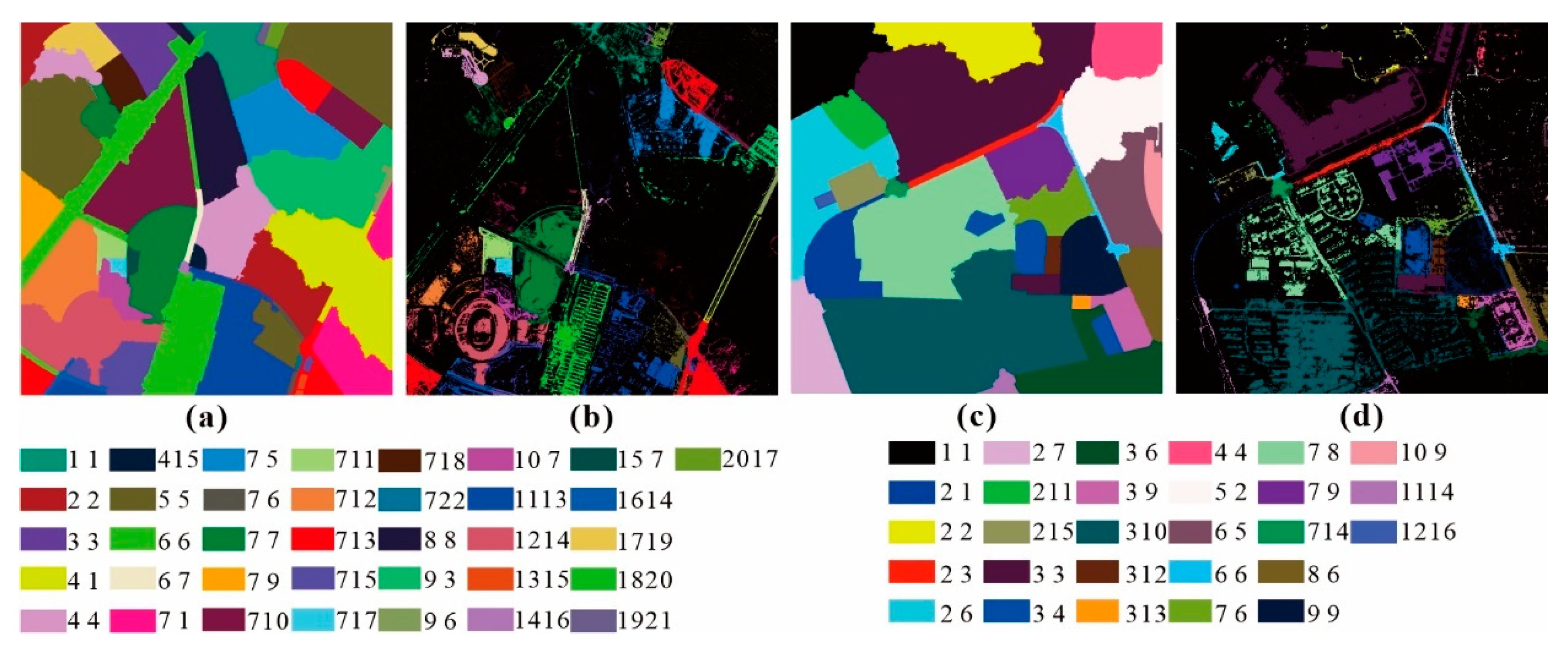
Figure 12.
Aerial image of an area in Dapeng, Shenzhen. (a) 2014. (b) 2017.

Figure 13.
The results of land-use types detected by CNNs (1: bare land, 3: park, 4: pond, 5: resort, 8: viaduct, 16: buildings, 21: commercial_area, 24: forest, 25: freeway, 26: golf_course, 29: industrial_area, 30: intersection, 32: lake, 33: meadow, 34: medium_residential, 35: mobile_home_park, 36: mountain, 37: overpass, 41: railway_station, 45: runway, 49: sparse_residential, 54: thermal_power_station, 55: wetland) (Experiment 2). (a) The category of the scene (2014). (b) The category of the scene (2017). (c) Information about scene changes.

Figure 14.
Schematic diagram of MST dividing training samples (Experiment 2). (a) The change intensity value of the spectrum. (b) MST divides the samples according to the value of the intensity of the change in the spectrum. (c) The change intensity value of the texture. (d) MST divides the samples according to the value of the intensity of the change in the texture.

Figure 15.
Training DBN and change range detection (Experiment 2). (a) The result of DBN model training. (b) Reference map. (c) The change detection result using a single threshold. (d) The change detection result using this paper method.
Figure 15.
Training DBN and change range detection (Experiment 2). (a) The result of DBN model training. (b) Reference map. (c) The change detection result using a single threshold. (d) The change detection result using this paper method.
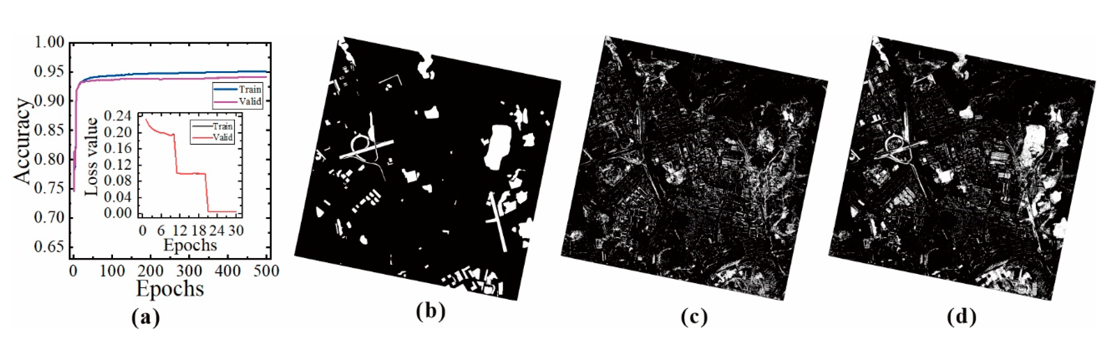
Figure 16.
Land use multi-type fine change detection results (Experiment 2). (a) Image of land change trajectory, where, image of 2014, 1: bare land, 2: medium_residential, 3: mountain, 4: railway_station, 5: industrial_area, 6: freeway, 7: pond, 8: dense_residential, 9: meadow, 10: sparse_residential, 11: viaduct, 12: commercial_area, 13: resort, 14: forest, 15: lake, 16: buildings, 17: intersection, 18: overpass, 19: park; image of 2017, 1: commercial_area, 2: medium_residential, 3: mountain, 4: railway_station, 5: industrial_area, 6: freeway, 7: pond, 8: dense_residential, 9: viaduct, 10: bare land, 11: resort, 12: forest, 13: meadow, 14: lake, 15: thermal_power_station, 16: buildings, 17: wetland, 18: intersection, 19: overpass, 20: park, 21: mobile_home_park, 22: runway. (b) Detail image.


Table 1.
Precision analysis (accuracy (A), recall (R), false alarm (FA), and missing alarm (MA)).
| Area | Method | A/% | R/% | FA/% | MA/% |
|---|---|---|---|---|---|
| Site1 | Single threshold | 68.39 | 41.78 | 59.92 | 58.22 |
| MST | 86.64 | 78.10 | 27.15 | 21.91 | |
| Site2 | Single threshold | 72.24 | 45.92 | 41.33 | 54.08 |
| MST | 84.98 | 81.49 | 25.75 | 18.51 |
Table 2.
Precision analysis (accuracy (A), recall (R), false alarm (FA), and missing alarm (MA)) (Experiment 2).
Table 2.
Precision analysis (accuracy (A), recall (R), false alarm (FA), and missing alarm (MA)) (Experiment 2).
| Method | A/% | R/% | FA/% | MA/% |
|---|---|---|---|---|
| Single threshold | 86.57 | 29.58 | 80.21 | 70.42 |
| MST | 91.57 | 77.10 | 55.60 | 22.93 |
© 2020 by the authors. Licensee MDPI, Basel, Switzerland. This article is an open access article distributed under the terms and conditions of the Creative Commons Attribution (CC BY) license (http://creativecommons.org/licenses/by/4.0/).
Share and Cite
MDPI and ACS Style
Wang, M.; Zhang, H.; Sun, W.; Li, S.; Wang, F.; Yang, G. A Coarse-to-Fine Deep Learning Based Land Use Change Detection Method for High-Resolution Remote Sensing Images. Remote Sens. 2020, 12, 1933. https://doi.org/10.3390/rs12121933
AMA Style
Wang M, Zhang H, Sun W, Li S, Wang F, Yang G. A Coarse-to-Fine Deep Learning Based Land Use Change Detection Method for High-Resolution Remote Sensing Images. Remote Sensing. 2020; 12(12):1933. https://doi.org/10.3390/rs12121933
Chicago/Turabian StyleWang, Mingchang, Haiming Zhang, Weiwei Sun, Sheng Li, Fengyan Wang, and Guodong Yang. 2020. "A Coarse-to-Fine Deep Learning Based Land Use Change Detection Method for High-Resolution Remote Sensing Images" Remote Sensing 12, no. 12: 1933. https://doi.org/10.3390/rs12121933
Note that from the first issue of 2016, this journal uses article numbers instead of page numbers. See further details here.